Equations of motion method for triplet excitation operators in graphene

Abstract

Particle-hole continuum in Dirac sea of graphene has a unique window underneath, which in principle leaves a room for bound state formation in the triplet particle hole channel [Phys. Rev. Lett. 89, 016402 (2002)]. In this work, we construct appropriate triplet particle-hole operators, and using a repulsive Hubbard type effective interaction, we employ equations of motions to derive approximate eigen-value equation for such triplet operators. While the secular equation for the spin density fluctuations gives rise to an equation which is second order in the strength of the short range interaction, the explicit construction of the triplet operators obtained here shows that in terms of these operators, the second order can be factorized to two first order equations, one of which gives rise to a solution below the particle-hole continuum of Dirac electrons in undoped graphene.

I Introduction

The single particle excitations in graphene and graphite are characterized by a Dirac cone Rotenberg ; Bostwick ; ARPESgraphite ; NetoRMP . As for the excitations in the two-quasi-particle sector, adding interactions may produce bound states in, especially particle-hole channel. Such bound states exhaust bosonic portion of excitation spectrum. In doped graphene, where an extended Fermi surface instead of Fermi points governs the continuum of free particle-hole excitations, the long range Coulomb forces binds initially free particle-hole pairs into spin singlet long lived bosonic excitations known as plasmons HwangSarma ; SeyllerHREELS . Now, let us think of what happens in the limit where doping tends to zero? In this limit the area of the Fermi circle becomes smaller and smaller, so that the ratio of Coulomb energy to the kinetic energy increases, and the single particle picture is expected to deviate from the simple Dirac cone, whereby signatures of correlation effect are expected to become important in the limit of undoped graphene.

The simplest model Hamiltonian which takes the dominant correlation effects into account is the Hubbard model. In the light of recent ab-initio estimates of the Hubbard $U$ in graphene, whose unscreened value can be as large as $\sim 10$ eV Wehling , it is important to examine possible consequences of such a large on-site interactions on the physical properties of graphene. Recently extensive quantum Monte Carlo (QMC) study of the phase diagram of the Hubbard model on the honeycomb lattice, suggests spin liquid ground state Meng for a range of $U/\gamma\sim 3-4$, ($\gamma$ being the nearest neighbor hopping amplitude). Therefore graphene is likely to be in the vicinity of a quantum spin liquid state Wehling . This scenario has been supported by other quantum Monte Carlo studies Azadi . Our recent QMC study suggests that the collective particle-hole excitations in $sp^{2}$ bonded planar systems are compatible with a picture based on spin charge separation Kaveh . In this scenario, the lowest excitations are triplet states which can be interpreted as two-spinon bound states. It is followed by a singlet excitation constructed from a doublon and a holon Vaezi . Moreover, lattice gauge theory simulation of $2+1$ dimensional QED predicts the critical value of the ”fine structure” constant in graphene can be crossed in suspended graphene Drut2009 . In this scenario, the ground state of graphene in vacuum is expected to be a Mott insulator, where in the ground state, the two-particle sector is dominated by long-range resonating valence bond correlations  Noorbakhsh . Therefore, despite an intriguing simplicity of the one-particle sector of excitations in graphene, the two-quasi-particle sector of excitations seems to be quite involved and may have remarkable singlet correlations in its ground state. Therefore it timely to revisit the nature of spin excitations in undoped graphene BaskaranJafari from weak coupling side which is describe by a Dirac liquid fixed point Jafari2009 .

The collective excitation considered here, will have distinct features from plasmons, because: (i) Formation of plasmons requires doping, while here we consider undoped graphene. (ii) Plasmons are formed in the singlet particle-hole channel, as a result of long range Coulomb forces. But here we assume a short range Hubbard type interaction, and focus on the triplet channel of particle-hole excitations. By constructing equations of motion DemlerZhang for triplet excitations formed across the valence and conduction band states in a Dirac cone, we obtain two triplet operators whose eigen-value equations are decoupled, and one of them displays solutions for finite values of the short range interaction strength. We compare our derivation with a naive RPA-like construction of a geometric series PeresComment , and show that for the triplet operators proposed in this work, the secular equation decouples into two first order equations in the short range interaction strength, one of which always does support a solution below the particle-hole continuum BaskaranJafari . Such a decoupling can not be achieved for spin density fluctuation operators PeresComment . Since these bosonic excitations are not precise spin density fluctuations, their coupling to neutrons is expected to be less than the coupling of spin density fluctuations. We therefore discuss the coupling of neutrons to such excitations.

II Effective Hamiltonian

As mentioned earlier, unlike plasmon (singlet) excitations, for which the long-range part of the Coulomb interaction is essential, since here we are interested in collective excitations in triplet (spin-flip) channel, we only need to consider the short range part of the interaction, as the spin-flip interactions are generated by short-range part of the interactions. It can be shown that inclusion of longer range part of the interactions does not lead to qualitative change in the dispersion of spin-1 collective excitations JafariBaskaran . Hence we start from the Hubbard model,

$$H =H_{0}+H_{U}$$ (1)

$$=-\gamma\sum_{\langle i,j\rangle,\sigma}\left(a^{\dagger}_{i\sigma}b_{j\sigma}+b^{\dagger}_{j\sigma}a_{i\sigma}\right)+U\sum_{j}n_{j\downarrow}n_{j\uparrow},$$

where $i,j$ denote sites of a honeycomb lattice, and $\sigma$ stands for spin of electrons. In this model, $U\sim 10$ eV is the bare value on-site Coulomb repulsion, and $\gamma\sim 2.5$ eV is the hopping amplitude to nearest neighbor sites. To be self-contained and to fix the notations, we briefly summarize the change of basis needed to diagonalize $H_{0}$. We introduce the Fourier transforms

$$a^{\dagger}_{j\sigma}=\frac{1}{\sqrt{N}}\sum_{{\vec{k}}}e^{-i{\vec{k}}.{\vec{R}}_{j}}a^{\dagger}_{{\vec{k}}\sigma}$$

$$b^{\dagger}_{j\sigma}=\frac{1}{\sqrt{N}}\sum_{{\vec{k}}}e^{-i{\vec{k}}.{\vec{R}}_{j+\delta}}b^{\dagger}_{{\vec{k}}\sigma}$$

where two atoms in the $j$’th unit cell are located at ${\vec{R}}_{j}$ ($\in A$) and ${\vec{R}}_{j+\delta}$ ($\in B$). $N$ is the the total number of cells. The above Fourier expansion, transforms the non-interacting part of the Hamiltonian to,

$$H_{0}=-\gamma\sum_{\langle i,j\rangle,\sigma}\Phi({\vec{k}})a^{\dagger}_{{\vec{k}}\sigma}b_{{\vec{k}}\sigma}+\Phi^{*}({\vec{k}})b^{\dagger}_{{\vec{k}}\sigma}a_{{\vec{k}}\sigma}$$ (2)

with the form factor given by,

$$\Phi({\vec{k}})=e^{i{\vec{k}}.\delta_{1}}+e^{i{\vec{k}}.\delta_{2}}+e^{i{\vec{k}}.\delta_{3}},$$ (3)

where $\delta_{1},\delta_{2},\delta_{3}$ are vectors connecting each atom in the $A$ sub-lattice to its nearest neighbors. The phase of the form factors are defined by $\gamma\Phi({\vec{k}})=\gamma|\Phi({\vec{k}})|e^{i\varphi_{{\vec{k}}}}\equiv\varepsilon_{{\vec{k}}}e^{i\varphi_{{\vec{k}}}}$, in terms of which the hopping term becomes,

$$H_{0}=-\sum_{{\vec{k}}\sigma}\varepsilon_{{\vec{k}}}\left(\begin{array}[]{cc}a^{\dagger}_{{\vec{k}}\sigma}&b^{\dagger}_{{\vec{k}}\sigma}\end{array}\right)\left(\begin{array}[]{cc}0&e^{i\varphi_{{\vec{k}}}}\\ e^{-i\varphi_{{\vec{k}}}}&0\end{array}\right)\left(\begin{array}[]{cc}a_{{\vec{k}}\sigma}\\ b_{{\vec{k}}\sigma}\end{array}\right)$$ (4)

The following change of basis from $(a,b)$ basis to $(c,v)$ basis,

$$\left(\begin{array}[]{cc}a_{{\vec{k}}\sigma}\\ b_{{\vec{k}}\sigma}\end{array}\right)=\frac{1}{\sqrt{2}}\left(\begin{array}[]{cc}1&1\\ e^{-i\varphi_{{\vec{k}}}}&-e^{-i\varphi_{{\vec{k}}}}\end{array}\right)\left(\begin{array}[]{cc}v_{{\vec{k}}\sigma}\\ c_{{\vec{k}}\sigma}\end{array}\right),$$ (5)

brings $H_{0}$ to diagonal format:

$$H_{0}=\sum_{{\vec{k}}\sigma}\varepsilon_{{\vec{k}}}\left(c^{\dagger}_{{\vec{k}}\sigma}c_{{\vec{k}}\sigma}-v^{\dagger}_{{\vec{k}}\sigma}v_{{\vec{k}}\sigma}\right).$$ (6)

Operators $c^{\dagger}_{{\vec{k}}\sigma}$ and $v_{{\vec{k}}\sigma}$ correspond to electron and hole operators. For later reference we note the explicit relation connecting $a^{\dagger}$ and $b^{\dagger}$ operators to these basis is given by,

$$a^{\dagger}_{j\sigma} = \frac{1}{\sqrt{N}}\sum_{{\vec{k}}}e^{i{\vec{k}}.{\vec{R}}_{j}}\frac{1}{\sqrt{2}}\left(v^{\dagger}_{{\vec{k}}\sigma}+c^{\dagger}_{{\vec{k}}\sigma}\right),$$ (7)

$$b^{\dagger}_{j\sigma} = \frac{1}{\sqrt{N}}\sum_{{\vec{k}}}e^{i{\vec{k}}.{\vec{R}}_{j+\delta}}e^{i\varphi_{{\vec{k}}}}\frac{1}{\sqrt{2}}\left(v^{\dagger}_{{\vec{k}}\sigma}-c^{\dagger}_{{\vec{k}}\sigma}\right).$$ (8)

Now let us rewrite the short range Hubbard interaction in the new basis in which $H_{0}$ is diagonal. The Hubbard interaction term in the exchange channel can be written as,

$$H_{U}=-U\sum_{j}a^{\dagger}_{j\uparrow}a_{j\downarrow}a^{\dagger}_{j\downarrow}a_{j\uparrow}+b^{\dagger}_{j\uparrow}b_{j\downarrow}b^{\dagger}_{j\downarrow}b_{j\uparrow}.$$ (9)

Upon using Eqns. (7) and (8) we have,

$$b^{\dagger}_{j\uparrow}b_{j\downarrow} = \frac{1}{2N}\sum_{{\vec{k}},{\vec{k}}^{\prime}}e^{i({\vec{k}}-{\vec{k}}^{\prime}).{\vec{R}}_{j+\delta}}e^{i\varphi_{{\vec{k}}}-i\varphi_{{\vec{k}}^{\prime}}}\left(v^{\dagger}_{{\vec{k}}\uparrow}-c^{\dagger}_{{\vec{k}}\uparrow}\right)\left(v_{{\vec{k}}^{\prime}\downarrow}-c_{{\vec{k}}^{\prime}\downarrow}\right)$$ (10)

$$b^{\dagger}_{j\downarrow}b_{j\uparrow} = \frac{1}{2N}\sum_{{\vec{p}},{\vec{p}}^{\prime}}e^{i({\vec{p}}-{\vec{p}}^{\prime}).{\vec{R}}_{j+\delta}}e^{i\varphi_{{\vec{p}}}-i\varphi_{{\vec{p}}^{\prime}}}\left(v^{\dagger}_{{\vec{p}}\downarrow}-c^{\dagger}_{{\vec{p}}\downarrow}\right)\left(v_{{\vec{p}}^{\prime}\uparrow}-c_{{\vec{p}}^{\prime}\uparrow}\right)$$ (11)

$$a^{\dagger}_{j\uparrow}a_{j\downarrow} = \frac{1}{2N}\sum_{{\vec{k}},{\vec{k}}^{\prime}}e^{i({\vec{k}}-{\vec{k}}^{\prime}).{\vec{R}}_{j}}\left(c^{\dagger}_{{\vec{k}}\uparrow}+v^{\dagger}_{{\vec{k}}\uparrow}\right)\left(c_{{\vec{k}}^{\prime}\downarrow}+v_{{\vec{k}}^{\prime}\downarrow}\right)$$ (12)

$$a^{\dagger}_{j\downarrow}a_{j\uparrow} = \frac{1}{2N}\sum_{{\vec{p}},{\vec{p}}^{\prime}}e^{i({\vec{p}}-{\vec{p}}^{\prime}).{\vec{R}}_{j}}\left(c^{\dagger}_{{\vec{p}}\downarrow}+v^{\dagger}_{{\vec{p}}\downarrow}\right)\left(c_{{\vec{p}}^{\prime}\uparrow}+v_{{\vec{p}}^{\prime}\uparrow}\right)$$ (13)

Inserting the above equations in the Hubbard term, $\frac{1}{N}\sum_{j}$ produces a momentum conservation constraint which can be satisfied by changing from ${\vec{k}}^{\prime}$ and ${\vec{p}}^{\prime}$ to a new variable ${\vec{q}}$ defined by

$${\vec{q}}\equiv{\vec{k}}-{\vec{k}}^{\prime}={\vec{p}}^{\prime}-{\vec{p}},$$ (14)

which eventually gives

$$H_{U} = -\frac{U}{4N}\sum_{{\vec{k}}{\vec{p}}{\vec{q}}}\left\{(c^{\dagger}_{{\vec{k}}\uparrow}+v^{\dagger}_{{\vec{k}}\uparrow})(c_{{\vec{k}}-{\vec{q}}\downarrow}+v_{{\vec{k}}-{\vec{q}}\downarrow})(c^{\dagger}_{{\vec{p}}\downarrow}+v^{\dagger}_{{\vec{p}}\downarrow})(c_{{\vec{p}}+{\vec{q}}\uparrow}+v_{{\vec{p}}+{\vec{q}}\uparrow})\right.$$ (15)

$$\left.+e^{i\varphi_{\vec{k}}-i\varphi_{{\vec{k}}-{\vec{q}}}+i\varphi_{\vec{p}}-i\varphi_{{\vec{p}}+{\vec{q}}}}(c^{\dagger}_{{\vec{k}}\uparrow}-v^{\dagger}_{{\vec{k}}\uparrow})(c_{{\vec{k}}-{\vec{q}}\downarrow}-v_{{\vec{k}}-{\vec{q}}\downarrow})(c^{\dagger}_{{\vec{p}}\downarrow}-v^{\dagger}_{{\vec{p}}\downarrow})(c_{{\vec{p}}+{\vec{q}}\uparrow}-v_{{\vec{p}}+{\vec{q}}\uparrow})\right\}$$

Expanding the Hubbard interaction in terms of electron ($c$) and hole ($v$) operators, generates $32$ terms. Combining the amplitudes $1$ and $e^{i\varphi_{\vec{k}}-i\varphi_{{\vec{k}}-{\vec{q}}}+i\varphi_{\vec{p}}-i\varphi_{{\vec{p}}+{\vec{q}}}}$ from first and second lines of Eq. (15), leads to $16$ types of terms with arbitrary number of electron and hole operators, whose amplitudes are of the form:

$$\gamma^{\pm}_{{\vec{k}}{\vec{p}}{\vec{q}}}\equiv\frac{1\pm e^{i\varphi_{\vec{k}}-i\varphi_{{\vec{k}}-{\vec{q}}}+i\varphi_{\vec{p}}-i\varphi_{{\vec{p}}+{\vec{q}}}}}{2}$$ (16)

As can be seen from Eq. (15), for those terms containing imbalanced number of $c$ and $v$ operators, the amplitude of the process generated by interaction will be $\gamma^{-}$, while for those where number of conduction and valence operators are balanced, the interaction vertex will be proportional to $\gamma^{+}$. Therefore in the long wave-length limit, $|\vec{q}|\to 0$, where $\gamma^{-}\to 0$, we expect the following types of terms to survive in the effective short range interaction:

$$\tilde{H}_{1}= -\frac{\tilde{U}}{2N}\sum_{{\vec{k}}{\vec{p}}{\vec{q}}}\gamma^{+}_{{\vec{k}}{\vec{p}}{\vec{q}}}~{}c^{\dagger}_{{\vec{k}}\uparrow}v_{{\vec{k}}-{\vec{q}}\downarrow}v^{\dagger}_{{\vec{p}}\downarrow}c_{{\vec{p}}+{\vec{q}}\uparrow}$$ (17)

$$\tilde{H}_{2}= -\frac{\tilde{U}}{2N}\sum_{{\vec{k}}{\vec{p}}{\vec{q}}}\gamma^{+}_{{\vec{k}}{\vec{p}}{\vec{q}}}~{}v^{\dagger}_{{\vec{k}}\uparrow}c_{{\vec{k}}-{\vec{q}}\downarrow}c^{\dagger}_{{\vec{p}}\downarrow}v_{{\vec{p}}+{\vec{q}}\uparrow}$$ (18)

$$\tilde{H}_{3}= -\frac{\tilde{U}}{2N}\sum_{{\vec{k}}{\vec{p}}{\vec{q}}}\gamma^{+}_{{\vec{k}}{\vec{p}}{\vec{q}}}~{}c^{\dagger}_{{\vec{k}}\uparrow}c_{{\vec{k}}-{\vec{q}}\downarrow}v^{\dagger}_{{\vec{p}}\downarrow}v_{{\vec{p}}+{\vec{q}}\uparrow}$$ (19)

$$\tilde{H}_{4}= -\frac{\tilde{U}}{2N}\sum_{{\vec{k}}{\vec{p}}{\vec{q}}}\gamma^{+}_{{\vec{k}}{\vec{p}}{\vec{q}}}~{}v^{\dagger}_{{\vec{k}}\uparrow}v_{{\vec{k}}-{\vec{q}}\downarrow}c^{\dagger}_{{\vec{p}}\downarrow}c_{{\vec{p}}+{\vec{q}}\uparrow}$$ (20)

$$\tilde{H}_{5}= -\frac{\tilde{U}}{2N}\sum_{{\vec{k}}{\vec{p}}{\vec{q}}}\gamma^{+}_{{\vec{k}}{\vec{p}}{\vec{q}}}~{}c^{\dagger}_{{\vec{k}}\uparrow}v_{{\vec{k}}-{\vec{q}}\downarrow}c^{\dagger}_{{\vec{p}}\downarrow}v_{{\vec{p}}+{\vec{q}}\uparrow}$$ (21)

$$\tilde{H}_{6}= -\frac{\tilde{U}}{2N}\sum_{{\vec{k}}{\vec{p}}{\vec{q}}}\gamma^{+}_{{\vec{k}}{\vec{p}}{\vec{q}}}~{}v^{\dagger}_{{\vec{k}}\uparrow}c_{{\vec{k}}-{\vec{q}}\downarrow}v^{\dagger}_{{\vec{p}}\downarrow}c_{{\vec{p}}+{\vec{q}}\uparrow}$$ (22)

There are two more terms with their vertex strength proportional to $\gamma^{+}$, namely $c^{\dagger}cc^{\dagger}c$ and $v^{\dagger}vv^{\dagger}v$ which correspond to particle-hole fluctuations solely in the conduction or valence band, which will not contribute in the undoped graphene, as average occupation numbers arising from the Hartree decomposition of the equations of motion (see the following section) makes them irrelevant at this mean field level. Beyond the mean field, they are supposed to renormalize the bare value of $U\to\tilde{U}$. Therefore the tree level effective short range Hamiltonian we use in this work is,

$$H^{\rm eff}=H_{0}+\sum_{\alpha=1}^{6}\tilde{H}_{\alpha}.$$ (23)

The bare value of $U\sim 4\gamma$ is expected to get renormalized to a smaller value $\tilde{U}\lesssim 2.23\gamma$, beyond which an instability occurs JafariBaskaran . The mean field factorization in the equation of motion employed here (next section) may lead to the underestimation of this upper value for $\tilde{U}$, which is a known effect of mean field treatments NagaosaBook . Therefore the physical range of parameters is limited to $\tilde{U}\sim 2\gamma$. More elaborate calculations based on exact diagonalization, as well as ab-initio quantum Monte Carlo calculation by us, supports the picture emerging from this effective Hamiltonian Kaveh . In the following section, we identify appropriate triplet operators, which satisfy a simple eigen-value equation, which correspond to singularities in the one-band RPA-type susceptibility.

III Construction of triplet operators

As a two-band generalization of the triplet excitation in YBCO superconductors DemlerZhang , consider two triplet operator defined for the particle-hole channel by,

$$c^{\dagger}_{{\tilde{k}}\uparrow}v_{{\tilde{k}}+{\tilde{q}}\downarrow},~{}~{}~{}~{}~{}~{}~{}~{}v^{\dagger}_{{\tilde{k}}\uparrow}c_{{\tilde{k}}+{\tilde{q}}\downarrow}.$$ (24)

These operators create triplet particle-hole excitations across the valence and conduction bands. Therefore, by construction, these operators are supposed to generate (triplet) excitations in undoped graphene. To study the dynamics of these triplet excitations we calculate their equation of motion in a normal state. In the right hand side of terms generated by the Hubbard interaction, we perform Hartree factorization in terms of appropriate occupation factors and the operator under study DemlerZhang . For $c^{\dagger}_{{\tilde{k}}\uparrow}v_{{\tilde{k}}+{\tilde{q}}\downarrow}$ excitations, non-zero contributions are generated by,

$$\left[H_{0},c^{\dagger}_{{\tilde{k}}\uparrow}v_{{\tilde{k}}+{\tilde{q}}\downarrow}\right]= \left(\varepsilon_{\tilde{k}}+\varepsilon_{{\tilde{k}}+{\tilde{q}}}\right)c^{\dagger}_{{\tilde{k}}\uparrow}v_{{\tilde{k}}+{\tilde{q}}\downarrow},$$ (25)

$$\left[\tilde{H}_{1},c^{\dagger}_{{\tilde{k}}\uparrow}v_{{\tilde{k}}+{\tilde{q}}\downarrow}\right]= -\frac{\tilde{U}}{2N}\left(\sum_{\vec{k}}\gamma^{+}_{{\vec{k}},{\tilde{k}}+{\tilde{q}},-{\tilde{q}}}c^{\dagger}_{{\vec{k}}\uparrow}v_{{\vec{k}}+{\tilde{q}}\downarrow}\right)(\bar{n}^{v}_{{\tilde{k}}+{\tilde{q}}\downarrow}-\bar{n}^{c}_{{\tilde{k}}\uparrow}),$$ (26)

$$\left[\tilde{H}_{6},c^{\dagger}_{{\tilde{k}}\uparrow}v_{{\tilde{k}}+{\tilde{q}}\downarrow}\right]= -\frac{\tilde{U}}{2N}\left(\sum_{\vec{k}}\gamma^{+}_{{\vec{k}},{\tilde{k}}+{\tilde{q}},-{\tilde{q}}}v^{\dagger}_{{\vec{k}}\uparrow}c_{{\vec{k}}+{\tilde{q}}\downarrow}\right)(\bar{n}^{v}_{{\tilde{k}}+{\tilde{q}}\downarrow}-\bar{n}^{c}_{{\tilde{k}}\uparrow}),$$ (27)

where a Hartree factorization in the right hand side has been performed to generate the average occupation numbers DemlerZhang . Similarly the non-zero contributions for triplet excitations from conduction to valence band after Hartree factorization become,

$$\left[H_{0},v^{\dagger}_{{\tilde{k}}\uparrow}c_{{\tilde{k}}+{\tilde{q}}\downarrow}\right]= -\left(\varepsilon_{\tilde{k}}+\varepsilon_{{\tilde{k}}+{\tilde{q}}}\right)v^{\dagger}_{{\tilde{k}}\uparrow}c_{{\tilde{k}}+{\tilde{q}}\downarrow}$$ (28)

$$\left[\tilde{H}_{2},v^{\dagger}_{{\tilde{k}}\uparrow}c_{{\tilde{k}}+{\tilde{q}}\downarrow}\right]= -\frac{\tilde{U}}{2N}\left(\sum_{\vec{k}}\gamma^{+}_{{\vec{k}},{\tilde{k}}+{\tilde{q}},-{\tilde{q}}}v^{\dagger}_{{\vec{k}}\uparrow}c_{{\vec{k}}+{\tilde{q}}\downarrow}\right)(\bar{n}^{c}_{{\tilde{k}}+{\tilde{q}}\downarrow}-\bar{n}^{v}_{{\tilde{k}}\uparrow})$$ (29)

$$\left[\tilde{H}_{5},v^{\dagger}_{{\tilde{k}}\uparrow}c_{{\tilde{k}}+{\tilde{q}}\downarrow}\right]= -\frac{\tilde{U}}{2N}\left(\sum_{\vec{k}}\gamma^{+}_{{\vec{k}},{\tilde{k}}+{\tilde{q}},-{\tilde{q}}}c^{\dagger}_{{\vec{k}}\uparrow}v_{{\vec{k}}+{\tilde{q}}\downarrow}\right)(\bar{n}^{c}_{{\tilde{k}}+{\tilde{q}}\downarrow}-\bar{n}^{v}_{{\tilde{k}}\uparrow})$$ (30)

The above set of results can be summarized as,

$$\left[H_{\rm eff},c^{\dagger}_{{\tilde{k}}\uparrow}v_{{\tilde{k}}+{\tilde{q}}\downarrow}\right] = \left(\varepsilon_{\tilde{k}}+\varepsilon_{{\tilde{k}}+{\tilde{q}}}\right)c^{\dagger}_{{\tilde{k}}\uparrow}v_{{\tilde{k}}+{\tilde{q}}\downarrow}-\frac{\tilde{U}}{2N}(\bar{n}^{v}_{{\tilde{k}}+{\tilde{q}}\downarrow}-\bar{n}^{c}_{{\tilde{k}}\uparrow})\sum_{\vec{k}}\gamma^{+}_{{\vec{k}},{\tilde{k}}+{\tilde{q}},-{\tilde{q}}}\left(c^{\dagger}_{{\vec{k}}\uparrow}v_{{\vec{k}}+{\tilde{q}}\downarrow}+v^{\dagger}_{{\vec{k}}\uparrow}c_{{\vec{k}}+{\tilde{q}}\downarrow}\right),$$ (31)

$$\left[H_{\rm eff},v^{\dagger}_{{\tilde{k}}\uparrow}c_{{\tilde{k}}+{\tilde{q}}\downarrow}\right] = -\left(\varepsilon_{\tilde{k}}+\varepsilon_{{\tilde{k}}+{\tilde{q}}}\right)v^{\dagger}_{{\tilde{k}}\uparrow}c_{{\tilde{k}}+{\tilde{q}}\downarrow}-\frac{\tilde{U}}{2N}\left(\bar{n}^{c}_{{\tilde{k}}+{\tilde{q}}\downarrow}-\bar{n}^{v}_{{\tilde{k}}\uparrow}\right)\sum_{\vec{k}}\gamma^{+}_{{\vec{k}},{\tilde{k}}+{\tilde{q}},-{\tilde{q}}}\left(c^{\dagger}_{{\vec{k}}\uparrow}v_{{\vec{k}}+{\tilde{q}}\downarrow}+v^{\dagger}_{{\vec{k}}\uparrow}c_{{\vec{k}}+{\tilde{q}}\downarrow}\right).$$ (32)

Here $H_{\rm eff}=\sum_{\alpha=0}^{6}H_{\alpha}$. Demanding right hand side of the above equations to be $\omega_{{\tilde{q}}}$ times $c^{\dagger}_{{\tilde{k}}\uparrow}v_{{\tilde{k}}+{\tilde{q}}\downarrow}$ and $v^{\dagger}_{{\tilde{k}}\uparrow}c_{{\tilde{k}}+{\tilde{q}}\downarrow}$, respectively, we obtain

$$\left(\omega_{\tilde{q}}-\varepsilon_{\tilde{k}}-\varepsilon_{{\tilde{k}}+{\tilde{q}}}\right)c^{\dagger}_{{\tilde{k}}\uparrow}v_{{\tilde{k}}+{\tilde{q}}\downarrow} = -\frac{\tilde{U}}{4N}\left(\bar{n}^{v}_{{\tilde{k}}+{\tilde{q}}\downarrow}-\bar{n}^{c}_{{\tilde{k}}\uparrow}\right)\sum_{\vec{k}}\left(1+\eta_{{\vec{k}},{\tilde{q}}}\eta^{*}_{{\tilde{k}},{\tilde{q}}}\right)\left(c^{\dagger}_{{\vec{k}}\uparrow}v_{{\vec{k}}+{\tilde{q}}\downarrow}+v^{\dagger}_{{\vec{k}}\uparrow}c_{{\vec{k}}+{\tilde{q}}\downarrow}\right)$$ (33)

$$\left(\omega_{\tilde{q}}+\varepsilon_{\tilde{k}}+\varepsilon_{{\tilde{k}}+{\tilde{q}}}\right)v^{\dagger}_{{\tilde{k}}\uparrow}c_{{\tilde{k}}+{\tilde{q}}\downarrow} = -\frac{\tilde{U}}{4N}\left(\bar{n}^{c}_{{\tilde{k}}+{\tilde{q}}\downarrow}-\bar{n}^{v}_{{\tilde{k}}\uparrow}\right)\sum_{\vec{k}}\left(1+\eta_{{\vec{k}},{\tilde{q}}}\eta^{*}_{{\tilde{k}},{\tilde{q}}}\right)\left(c^{\dagger}_{{\vec{k}}\uparrow}v_{{\vec{k}}+{\tilde{q}}\downarrow}+v^{\dagger}_{{\vec{k}}\uparrow}c_{{\vec{k}}+{\tilde{q}}\downarrow}\right).$$ (34)

with $\eta_{{\vec{k}},{\vec{q}}}\equiv e^{i\varphi_{{\vec{k}}}-i\varphi_{{\vec{k}}+{\vec{q}}}}$, which satisfies the property $\eta_{{\vec{k}},{\vec{q}}}^{-1}=\eta^{*}_{{\vec{k}},{\vec{q}}}=\eta_{-{\vec{k}},-{\vec{q}}}$. These set of equations suggest to define the following operators:

$${\cal O}_{{\tilde{q}}} \equiv\sum_{{\vec{k}}}\left(c^{\dagger}_{{\vec{k}}\uparrow}v_{{\vec{k}}+{\tilde{q}}\downarrow}+v^{\dagger}_{{\vec{k}}\uparrow}c_{{\vec{k}}+{\tilde{q}}\downarrow}\right),$$ (35)

$$\bar{\cal O}_{{\tilde{q}}} \equiv\sum_{{\vec{k}}}\left(c^{\dagger}_{{\vec{k}}\uparrow}v_{{\vec{k}}+{\tilde{q}}\downarrow}+v^{\dagger}_{{\vec{k}}\uparrow}c_{{\vec{k}}+{\tilde{q}}\downarrow}\right)\eta_{{\vec{k}},{\tilde{q}}}.$$ (36)

The eigen-value problem for these operators become,

$${\cal O}_{\tilde{q}} =\tilde{U}\chi_{0}({\tilde{q}}){\cal O}_{{\tilde{q}}}+\tilde{U}\bar{\chi}_{0}^{\prime}({\tilde{q}})\bar{\cal O}_{\tilde{q}},$$ (37)

$$\bar{\cal O}_{\tilde{q}} =\tilde{U}\bar{\chi}_{0}({\tilde{q}}){\cal O}_{{\tilde{q}}}+\tilde{U}\chi_{0}({\tilde{q}})\bar{\cal O}_{\tilde{q}},$$ (38)

where

$$\chi_{0}({\tilde{q}})\!\! = \!\!-\frac{1}{4N}\sum_{{\tilde{k}}}\left(\frac{\bar{n}^{v}_{{\tilde{k}}+{\tilde{q}}\downarrow}-\bar{n}^{c}_{{\tilde{k}}\uparrow}}{\omega_{\tilde{q}}-\varepsilon_{\tilde{k}}-\varepsilon_{{\tilde{k}}+{\tilde{q}}}}+\frac{\bar{n}^{c}_{{\tilde{k}}+{\tilde{q}}\downarrow}-\bar{n}^{v}_{{\tilde{k}}\uparrow}}{\omega_{\tilde{q}}+\varepsilon_{\tilde{k}}+\varepsilon_{{\tilde{k}}+{\tilde{q}}}}\right)$$ (39)

$$\bar{\chi}_{0}({\tilde{q}})\!\! = \!\!-\frac{1}{4N}\sum_{{\tilde{k}}}\left(\frac{\bar{n}^{v}_{{\tilde{k}}+{\tilde{q}}\downarrow}-\bar{n}^{c}_{{\tilde{k}}\uparrow}}{\omega_{\tilde{q}}-\varepsilon_{\tilde{k}}-\varepsilon_{{\tilde{k}}+{\tilde{q}}}}+\frac{\bar{n}^{c}_{{\tilde{k}}+{\tilde{q}}\downarrow}-\bar{n}^{v}_{{\tilde{k}}\uparrow}}{\omega_{\tilde{q}}+\varepsilon_{\tilde{k}}+\varepsilon_{{\tilde{k}}+{\tilde{q}}}}\right)\eta_{{\tilde{k}},{\tilde{q}}},$$

$$\bar{\chi}_{0}^{\prime}({\tilde{q}})\!\! = \!\!-\frac{1}{4N}\sum_{{\tilde{k}}}\left(\frac{\bar{n}^{v}_{{\tilde{k}}+{\tilde{q}}\downarrow}-\bar{n}^{c}_{{\tilde{k}}\uparrow}}{\omega_{\tilde{q}}-\varepsilon_{\tilde{k}}-\varepsilon_{{\tilde{k}}+{\tilde{q}}}}+\frac{\bar{n}^{c}_{{\tilde{k}}+{\tilde{q}}\downarrow}-\bar{n}^{v}_{{\tilde{k}}\uparrow}}{\omega_{\tilde{q}}+\varepsilon_{\tilde{k}}+\varepsilon_{{\tilde{k}}+{\tilde{q}}}}\right)\eta^{*}_{{\tilde{k}},{\tilde{q}}}.$$

In the last equation, since $\eta^{*}_{{\vec{k}},{\tilde{q}}}=\eta_{-{\vec{k}},-{\tilde{q}}}$, and the fractions under the parenthesis are invariant with respect to inversion of the vectors ${\vec{k}}$ and ${\vec{k}}+{\tilde{q}}$, we conclude that $\bar{\chi}_{0}=\bar{\chi}_{0}^{\prime}$. Hence eigenvalue equations decouple into the following equations for the symmetric and antisymmetric modes constructed from ${\cal O}$ and $\bar{\cal O}$ triplet operators:

$${\cal T}_{{\tilde{q}}}^{\pm}\left(1-\tilde{U}(\chi_{0}\pm\bar{\chi}_{0})\right)=0.$$ (40)

where the normalized form of our triplet operator ${\cal T}_{\tilde{q}}^{\pm}={\cal O}_{\tilde{q}}\pm\bar{\cal O}_{\tilde{q}}$ is given by,

$${\cal T}_{{\tilde{q}}}^{\pm}\equiv\frac{1}{{\cal N}^{\pm}_{\tilde{q}}}\sum_{{\vec{k}}}\left(c^{\dagger}_{{\vec{k}}\uparrow}v_{{\vec{k}}+{\tilde{q}}\downarrow}+v^{\dagger}_{{\vec{k}}\uparrow}c_{{\vec{k}}+{\tilde{q}}\downarrow}\right)(1\pm\eta_{{\vec{k}},{\tilde{q}}}).$$ (41)

The normalization factor satisfies,

$$\left({\cal N}^{\pm}_{\tilde{q}}\right)^{2}=4\sum_{\vec{k}}\left(1\pm\cos(\varphi_{\vec{k}}-\varphi_{{\vec{k}}+{\tilde{q}}})\right)$$ (42)

Since we are dealing with undoped graphene, and assuming the temperature to be zero, the occupation numbers in the conduction and valence bands will be $0$ and $1$, respectively. Therefore, the susceptibility corresponding to the above operators reduces to,

$$\chi_{0}({\tilde{q}})\pm\bar{\chi}_{0}({\tilde{q}})=\frac{1}{4N}\sum_{{\vec{k}}}$$ (43)

$$\left(\frac{1}{\omega_{\tilde{q}}-\varepsilon_{\vec{k}}-\varepsilon_{{\vec{k}}+{\tilde{q}}}+i0}-\frac{1}{\omega_{\tilde{q}}+\varepsilon_{\vec{k}}+\varepsilon_{{\vec{k}}+{\tilde{q}}}-i0}\right)(1\pm\eta_{{\vec{k}},{\vec{q}}})$$

In the low-energy limit where the Dirac cone linearization of the spectrum is valid, these integrals in the the particle-hole fluctuation can be analytically performed Wunsch ; HwangSarma . Otherwise they can be computed with standard numerical procedures. Let us present here a geometric arguments based on a very peculiar constraint in the k-space which arises from the conic spectrum. Chiral nature of one particle eigen states, implies that the back-scattering will not be allowed for scattering of two electrons or two holes. However, for the scattering of a particle and a hole, the very same chiral nature according to which the matrix elements between a hole and an electron state is proportional to $1-e^{i\varphi_{{\vec{k}}}-i\varphi_{{\vec{k}}+{\vec{q}}}}$, enhances the back-scattering between the particle and a hole. In the small ${\vec{q}}$ limit as in Fig. 1, the contributions to the imaginary part of integrals in Eq. (43) comes from a set of points on the ellipse defined by $\omega_{\tilde{q}}=v_{F}(|{\vec{k}}|+|{\vec{k}}+{\vec{q}}|)$. Enhanced back-scattering in the particle-hole channel in the above geometry corresponds to the limit where ellipse degenerates into two almost parallel line segments, i.e. the limit $\omega_{\vec{q}}\approx v_{F}|{\vec{q}}|$. This limit corresponds to the lower edge of the particle-hole continuum where indeed a dominant inverse square root behavior (see Eq. 45) describes the non-interacting susceptibility HwangSarma ; BaskaranJafari . Such a geometrical constraint in the phase space could be considered as a novel rout to 2D bosonization scheme which may find applications in systems with Dirac cone, such as graphene and topological insulators HasanKane .

Now let us study the behavior of susceptibilities corresponding to the two triplet operators obtained here with the aid of the geometrical argument introduced above. In this limit the ellipse tends to two line which enforces ${\vec{k}}$ and ${\vec{k}}+{\vec{q}}$ to be in opposite directions, such that, $1\pm\eta_{{\vec{k}},{\vec{q}}}=1\pm e^{i\varphi_{{\vec{k}}}-i\varphi_{{\vec{k}}+{\vec{q}}}}\to 1\pm e^{i\pi}$. Therefore in the small ${\tilde{q}}$ limit, $\chi_{0}({\tilde{q}})+\bar{\chi}_{0}({\tilde{q}})$ vanishes, and a very large value of $\tilde{U}$ will be required to excite the ${\cal T}_{\tilde{q}}^{+}$. Hence, as long as we are interested in solutions for finite values of $\tilde{U}$, we are left with the triplet operator ${\cal T}^{-}_{\tilde{q}}$ whose eigenvalue equation can be simplified to:

$$1-\tilde{U}\tilde{\chi}_{0}({\tilde{q}})=0,~{}~{}~{}~{}~{}~{}~{}~{}~{}~{}\tilde{\chi}_{0}({\tilde{q}})=\frac{1}{2N}\sum_{\vec{k}}$$ (44)

$$\left(\frac{1}{\omega_{\tilde{q}}-\varepsilon_{\vec{k}}-\varepsilon_{{\vec{k}}+{\tilde{q}}}}-\frac{1}{\omega_{\tilde{q}}+\varepsilon_{\vec{k}}+\varepsilon_{{\vec{k}}+{\tilde{q}}}}\right)\frac{1-\cos(\varphi_{\vec{k}}-\varphi_{{\vec{k}}+{\tilde{q}}})}{2}$$

where we have used the symmetry of the bosonic propagator under the inversion symmetry (in ${\vec{k}}$ space) to project out the even part of the $1-e^{i\varphi_{\vec{k}}-i\varphi_{{\vec{k}}+{\tilde{q}}}}$ factor.

Figure 1: Points in $\vec{k}$-space located on the ellipse contribute in the delta function integration of $\Im\tilde{\chi}_{0}$. In $\hbar\omega\to v_{F}|\vec{q}|\to 0$ limit the ellipse degenerates into two line segments where $\vec{k}$ and $\vec{k}^{\prime}=\vec{k}+\vec{q}$ point in the opposite direction; $\theta_{\vec{k}}-\theta_{\vec{k}^{\prime}}\to\pi$. Hence the overlap factors in this limit tend to a trivial factor of $1$ and become irrelevant.

As we mentioned, closed form formula for the above particle-hole fluctuation can be obtained Wunsch ; HwangSarma ,

$$\tilde{\chi}_{0}({\tilde{q}},\omega)=\frac{{\tilde{q}}^{2}}{16}\frac{1}{\sqrt{v_{F}^{2}{\tilde{q}}^{2}-\omega^{2}}},$$ (45)

which despite ignoring phase factors $(1-\eta_{{\vec{k}},{\tilde{q}}})$ is identical to the result obtained in Ref. BaskaranJafari . The fact that ignoring these phase factors in Ref. BaskaranJafari in undoped graphene, does not change the low-energy behavior lends on the particular geometry arising from chiral nature of single-particle states (Fig. 1). However, for the case of doped graphene, one has to properly take them into account, even for short range interactions MoradDoped .

The eigenvalue equation for ${\cal T}_{{\tilde{q}}}^{-}$ is equivalent to divergence in the triplet susceptibility at random phase approximation BickersScalapino ,

$$\chi^{\rm RPA}_{\rm triplet}({\tilde{q}},\omega)=\frac{\tilde{\chi}_{0}({\tilde{q}},\omega)}{1-\tilde{U}\tilde{\chi}_{0}({\tilde{q}},\omega)},$$ (46)

where retarded bare susceptibility $\chi_{0,\alpha\alpha^{\prime}}({\tilde{q}},\omega)$ in our notation is given by the standard particle-hole form HwangSarma ,

$$\frac{1}{2N}\sum_{{\vec{k}}}\frac{(\bar{n}^{\alpha^{\prime}}_{\vec{k}+{\tilde{q}}}-\bar{n}^{\alpha}_{\vec{k}})\left(1+{\alpha\alpha^{\prime}}\cos(\varphi_{{\vec{k}}}-\varphi_{{\vec{k}}+{\tilde{q}}})\right)}{\hbar\omega-(\alpha^{\prime}\varepsilon_{{{\vec{k}}+{\tilde{q}}}}-\alpha\varepsilon_{{\vec{k}}})+i0^{+}}.$$ (47)

Here $\alpha,\alpha^{\prime}$ take $\pm$ values corresponding to conduction and valence bands, respectively HwangSarma . To understand the origin of overlap factors in this expression we note that the matrix elements of the scattering interaction $V$ between chiral states $(\vec{k},\alpha)$ and $(\vec{k}^{\prime},\alpha^{\prime})$ of the cone-like dispersion in graphene are given by $\langle\vec{k}^{\prime},\alpha^{\prime}|V|\vec{k},\alpha\rangle=\tilde{V}(\vec{k}-\vec{k}^{\prime})\left(1+\alpha\alpha^{\prime}e^{i\varphi_{\vec{k}}-i\varphi_{\vec{k}^{\prime}}}\right)/2$, where $\tilde{V}$ is the Fourier transform of the scattering potential. When the above phase factors are inserted into particle-hole bubble diagrams, give rise to the overlap factor in the free particle-hole propagator, Eq. (47). Therefore, despite that the operators considered here are not exactly what one expects from a local spin fluctuation operator, nevertheless, the susceptibility corresponding to them is the particle-hole bubble. But the main difference between spin density fluctuation and our triplet operators is that the former satisfies a second order equation in $\tilde{U}$ which does not have a solution PeresComment , while our triplet operators satisfy two first order equations, one of which as will be shown below has a solution below the continuum of free particle-hole excitations BaskaranJafari .

IV Short range versus long range interactions

To emphasize the importance of Eq. (40) for short range interactions, let us discuss how one obtains a matrix form for the spin density fluctuation which then leads to a second order secular equation PeresComment . When the range of interactions is so short that the two neighboring atoms from two sub-lattices A, B can be resolved, an RPA like geometric series for the susceptibility gives rise to the following equations:

$$\chi_{AA} =\chi^{0}_{AA}+\tilde{U}\chi^{0}_{AA}\chi_{AA}+\tilde{U}\chi^{0}_{AB}\chi_{BA}$$

$$\chi_{AB} =\chi^{0}_{AB}+\tilde{U}\chi^{0}_{AA}\chi_{AB}+\tilde{U}\chi^{0}_{AB}\chi_{BB}$$

$$\chi_{BA} =\chi^{0}_{BA}+\tilde{U}\chi^{0}_{BA}\chi_{AA}+\tilde{U}\chi^{0}_{BB}\chi_{BA}$$

$$\chi_{BB} =\chi^{0}_{BB}+\tilde{U}\chi^{0}_{BA}\chi_{AB}+\tilde{U}\chi^{0}_{BB}\chi_{BB}$$

where due to short range interaction $U$, the Hubbard interaction connects $\chi^{0}\chi$ products in a manner that their internal indices are the same (Fig. 2). The above set of equations decouples and gives two sets of determinants of the following form,

$$\left|\begin{array}[]{cc}1-\tilde{U}\chi^{0}_{AA}&-\tilde{U}\chi^{0}_{AB}\\ -\tilde{U}\chi^{0}_{BA}&1-\tilde{U}\chi^{0}_{BB}\end{array}\right|=0,$$ (48)

which is a quadratic equation obtained by constructing RPA-like series of Feynman diagrams for particle-hole pairs propagating between the lattice sites. This condition corresponds to the poles in the RPA susceptibility of spin density fluctuations, which will not lead to any solution (bound state) PeresComment .

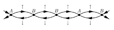
Figure 2: Typical geometric series for short range interactions where the bubbles meet either on A, or B sites. Therefore internal indices for short range interactions become identical.

To see why the second order equation is peculiar to short range interactions, consider long range interactions, for which one can construct the following geometric series,

$$\chi_{AA} = \chi^{0}_{AA}+W\sum_{m,m^{\prime}}\chi^{0}_{Am}\chi_{m^{\prime}A}$$

$$\chi_{AB} = \chi^{0}_{AB}+W\sum_{m,m^{\prime}}\chi^{0}_{Am}\chi_{m^{\prime}B}$$

$$\chi_{BA} = \chi^{0}_{BA}+W\sum_{m,m^{\prime}}\chi^{0}_{Bm}\chi_{m^{\prime}A}$$

$$\chi_{BB} = \chi^{0}_{BB}+W\sum_{m,m^{\prime}}\chi^{0}_{Bm}\chi_{m^{\prime}B}.$$

Here due to long-range interaction $W$, the indices $m,m^{\prime}$ are not necessarily identical, and they can take both $A$ and $B$ values, as the long range interaction treats both indices on the same footing. Summing all these equations, we can see that a symmetric mode decouples from the rest of equations, which satisfies the following equation:

$$1-W(\chi^{0}_{AA}+\chi^{0}_{AB}+\chi^{0}_{BA}+\chi^{0}_{BB})=0,$$ (49)

which is first order in the (long range) interaction strength, $W$. Therefore, the factorization of the eigenvalue equation into first order equations in presence of short range interactions discussed for our triplet operators is not trivial, and is a consequence of the peculiar form of these operators. If one writes down the spin density operator, e.g. Eq. (55), one can see that the operators considered here do not precisely correspond to spin density fluctuations. Spin density fluctuations in presence of short range interactions give rise to a second order equation as argued above PeresComment . However, a judicious choice of ${\cal T}^{\pm}_{{\tilde{q}}}$ operators done here, manages to decouple an equation which otherwise is expected to be second order, into two first order equations. This argument not only presents the explicit formula for the triplet fluctuations, but also supports our earlier prediction of neutral triplet excitations in undoped graphene and graphite BaskaranJafari .

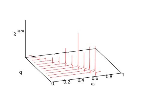
Figure 3: (Color online) Plot of the real part of RPA-like expression in undoped graphene, for $\tilde{U}=1.9\gamma$. The blank region in $\omega-q$ plane corresponding to higher values of $\omega$ is the particle-hole continuum, where the imaginary part of $\chi^{0}$ becomes non-zero. As can be seen, a singularity in the the RPA susceptibility below the particle-hole continuum occurs, which indicates vanishing of the RPA denominator, which is nothing but solution of the eigen-value equation for the triplet collective excitation. Energies are in units of $\gamma$.

V Neutron scattering cross section

Using Eq. (45) to solve the eigen-value equation (44), gives the following dispersion for the collective triplet excitations BaskaranJafari ,

$$\omega({\tilde{q}})=v_{F}{\tilde{q}}-\frac{\tilde{U}^{2}}{32v_{F}}{\tilde{q}}^{3},$$ (50)

which is valid in the limit where Dirac cone linearization applies. When the entire band dispersion is used, one can perform the integrals numerically. The solutions of the eigenvalue equation (40) for ${\cal T}^{-}_{\tilde{q}}$ operator, can be visualized as singularities in an RPA-like susceptibility $\tilde{\chi}_{0}/(1-\tilde{U}\tilde{\chi}_{0})$. In Fig. 3 we have plotted the real part of the above RPA-like expression for few values of ${\tilde{q}}$ and a typical value of $\tilde{U}=1.9\gamma$. The location of sharp divergences in the horizontal plane in this plot represents the dispersion of the neutral triplet collective excitation generated by ${\cal T}^{-}_{{\tilde{q}}}$.

The Dirac cone description of the electronic states of graphene equally holds in graphite, as long as one is interested in energy scales above the inter-layer hopping, $t_{\perp}\sim 50$ meV. The Dirac cone description of the electronic states is valid in length scales much larger than the lattice spacing. Therefore, even in highly oriented pyrolitic graphite (HOPG) where various planes might be slightly rotated around the $z$-axis with respect to each other, anisotropy in the momentum space can be safely ignored and still a Dirac cone description will remain valid. Hence our formulation of the spin-1 collective excitations is not only relevant to graphene, but also will be relevant to graphite and HOPG at energy scales above the inter-layer hopping. For such bulk samples, one may think of neutron scattering to search for the spin-1 collective excitations. However, since the operator corresponding to the triplet excitation is not identical to the spin density fluctuations, the coupling of neutrons is expected to be renormalized by appropriate matrix elements. Therefore in this section, we consider the behavior of neutron peak intensity in the limit of small ${\tilde{q}}$, with explicitly taking our triplet operators into account.

In polarized neutron scattering experiments, one measures,

$$S({\tilde{q}},\omega)=\sum_{n}|\langle 0|S^{-}_{\tilde{q}}|n\rangle|^{2}\delta\left(\omega-\omega_{n0}\right)$$ (51)

where $|0\rangle$ and $|n\rangle$ are ground and excited states of the whole system. As discussed in this paper, a class of approximate excitations are given by

$$|n\rangle=\frac{1}{{\cal N}^{-}_{\tilde{q}}}{\cal T}^{-}_{\tilde{q}}|0\rangle$$ (52)

where the normalization factor $1/{\cal N}^{-}_{\tilde{q}}$ has been defined by Eq. (42). Contribution of this class of excitations to the structure factor will be given by

$$S_{\rm triplet}({\tilde{q}},\omega) = \frac{1}{{\cal N}_{\tilde{q}}^{2}}\left|\langle 0|S^{-}_{\tilde{q}}{\cal T}^{-}_{\tilde{q}}|0\rangle\right|^{2}\delta(\omega-\omega_{\tilde{q}})$$

$$= \frac{1}{{\cal N}_{\tilde{q}}^{2}}\left|\langle 0|[S^{-}_{\tilde{q}},{\cal T}^{-}_{\tilde{q}}]|0\rangle\right|^{2}\delta(\omega-\omega_{\tilde{q}})$$

where we have used the fact that there are no triplet excitations in the ground state: $\langle 0|{\cal T}^{-}_{\tilde{q}}=0$. Moreover, note that here we need the vacuum expectation value of the ${\cal T}^{-}_{\tilde{q}}$, so that the $v^{\dagger}_{\uparrow}c_{\downarrow}$ term gives zero when acting on $|0\rangle$. Hence in the calculation of commutators, we drop the $c^{\dagger}_{\uparrow}v_{\downarrow}$ part of the triplet operator. The spin-flip operator in the present two-band situation is given by

$$S^{-}_{{\tilde{q}},a} =\frac{1}{2\sqrt{N}}\sum_{\vec{p}}\left(v^{\dagger}_{{\vec{p}}\downarrow}+c^{\dagger}_{{\vec{p}}\downarrow}\right)\left(v_{{\vec{p}}-{\tilde{q}}\uparrow}+c_{{\vec{p}}-{\tilde{q}}\uparrow}\right)$$ (54)

$$S^{-}_{{\tilde{q}},b} =\frac{1}{2\sqrt{N}}\sum_{\vec{p}}e^{i\varphi_{\vec{p}}-i\varphi_{{\vec{p}}-{\tilde{q}}}}\left(v^{\dagger}_{{\vec{p}}\downarrow}-c^{\dagger}_{{\vec{p}}\downarrow}\right)\left(v_{{\vec{p}}-{\tilde{q}}\uparrow}-c_{{\vec{p}}-{\tilde{q}}\uparrow}\right)$$ (55)

The required commutators will become

$$\langle\left[S^{-}_{{\tilde{q}},a},{\cal T}^{-}_{\tilde{q}}\right]\rangle = \frac{1}{\sqrt{N}}\sum_{\vec{k}}\left(1-\eta_{{\vec{k}},{\tilde{q}}}\right)\left(\langle v^{\dagger}_{{\vec{k}}+{\tilde{q}}\downarrow}v_{{\vec{k}}+{\tilde{q}}\downarrow}-c^{\dagger}_{{\vec{k}}\uparrow}c_{{\vec{k}}\uparrow}\rangle\right)$$

$$\left[S^{-}_{{\tilde{q}},b},{\cal T}^{-}_{\tilde{q}}\right] = -\left[S^{-}_{{\tilde{q}},a},{\cal T}^{-}_{\tilde{q}}\right]^{*}$$ (56)

At zero temperature, the conduction band is empty and the valence band is completely filled, so that the intensity of the mode will be given by

$$\frac{1}{{\cal N}^{2}_{{\tilde{q}}}}\left|\sum_{{\vec{k}}}(1-\eta_{{\vec{k}},{\tilde{q}}})\right|^{2}\sim\frac{|{\tilde{q}}^{2}|^{2}}{{\tilde{q}}^{2}}\sim{\tilde{q}}^{2}$$ (57)

where the asymptotic expressions for the integrals required above are obtained with the aid of the following expansion:

$$|{\vec{k}}+{\tilde{q}}|=k+\hat{k}.{\tilde{q}}+\frac{1}{2k}[{\tilde{q}}^{2}-({\tilde{q}}.\hat{k})^{2}]+{\cal O}({\tilde{q}}^{3})$$ (58)

The $\propto{\tilde{q}}^{2}$ behavior of the neutron scattering intensity makes the direct observation of such quanta of triplet excitations challenging for neutron scattering experiments. Optimum spots for a neutron scattering experiments are away from the $\Gamma$ point JafariBaskaran . Moreover, due to vanishingly small binding energy of the triplet excitations with respect to the lower boundary of the particle-hole continuum in Fig. 3, the resulting neutron peak even if observed, maybe washed by broad spectra of the adjacent free particle-hole pairs. Therefore a gap opening mechanism in graphite (such as proximity to a superconducting condensate, etc.) can be helpful in separating the energy scales associated with the expected sharp resonance peak from broad features associated with the continuum of incoherent excitations.

VI Summary and discussions

The secular equation obtained by Peres and coworkers PeresComment for spin density fluctuations in presence of short range interactions, is second order in $\tilde{U}$, which does not admit a solution. However, here instead of second order equation, we obtain two set of first order equations for ${\cal T}^{\pm}_{{\tilde{q}}}$ operators, one of which (${\cal T}^{+}_{{\tilde{q}}}$) does not lead to split-off state for finite $\tilde{U}$, while the other (${\cal T}^{-}_{{\tilde{q}}}$) satisfying a first order equation leads to a dispersive triplet collective excitations whose energy band-width is on the scale of the hopping amplitude $\gamma$. Such a bosonic branch of excitations might be responsible for: (i) The life-time anomaly observed in time resolved photo-emission spectroscopy of highly oriented pyrolytic graphite Ebrahimkhas . (ii) The kink observed in the dispersion of Dirac electrons in nearly free standing graphene samples kink . (iii) The spin-flip excitations observed in artificial honeycomb lattice formed by quantum dots vittore . The interpretation of such triplet mode as weak coupling analogue of two-spinon bound states has been supported by some recent Monte Carlo calculations Azadi ; Kaveh . Despite intriguing simplicity of the Dirac cone for the single-particle excitations of graphene/HOPG, it appears that the particle-hole sector of excitations is likely to be more involved, and short-range and/or Heisenberg forms of interactions maybe needed to capture the underlying singlet correlations Azadi ; Meng .

VII acknowledgments

We thank K. Yamada for fruitful discussions, and hospitality at IMR, Tohoku University. S.A.J. was supported by the National Elite Foundation (NEF) of Iran.

References

• (1) A. Bostwick, T. Ohta, T. Seyller, K. Horn, and E. Rotenberg. Nature Physics 3, 36 (2007)
• (2) A. Bostwick, T. Ohta, J. L. McChesney, T. Seyller, K. Horn, E. Rotenberg, Solid State Commun. 143, 63 (2007).
• (3) For a review see: A. H. Castro Neto, F. Guinea, N. M. R. Peres, K. S. Novoselov, A. K. Geim, Rev. Mod. Phys. 81, 109 (2009).
• (4) S. Y. Zhou, G.-H. Gweon, J. Graf, A. V. Fedorov, C. D. Spataru, R. D. Diehl, Y. Kopelevich, D.-H. Lee, Steven G. Louie, A. Lanzara, Nat. Phys. 2, 595 (2006).
• (5) A. H. Hwang, D. Sarma, Phys. Rev. B 75, 205418 (2006).
• (6) Yu Liue, R. F. Willis, K. V. Emtsev and Th. Seyller, Phys. Rev. B 78, 201403 (2008).
• (7) T. O. Wehling, E. Sasioglu, C. Friedrich, A. I. Lichtenstein, M. I. Katsnelson, and S. Bluügel, arXiv:1101.4007 (2011).
• (8) Z. Y. Meng, T. C. Lang, S. Wessel, F. F. Assaad, and A. Muramatsu, Nature 462, 847 (2010).
• (9) M. Marchi, S. Azadi, S. Sorella, Phys. Rev. Lett. 107 086807 (2011).
• (10) K. H. Mood, S. A. Jafari, E. Adibi, G. Baskaran, M. R. Abolhassani, arxiv:1107.4208 (2011).
• (11) A. Vaezi, X. G. Wen, arXiv:1010.5744 (2010).
• (12) J. E. Drut, and T. A. Lahde, Phys. Rev. Lett. 102, 026802 (2009); J. E. Drut and T. A. Lahde, Phys. Rev. B 79, 165425 (2009).
• (13) Z. Noorbakhsh, F. Shahbazi, S. A. Jafari and G. Baskaran, J. Phys. Soc. Jpn. 78, 054701 (2009).
• (14) G. Baskaran, S.A. Jafari, Phys. Rev. Lett. 89, 016402 (2002); G. Baskaran, S.A. Jafari, Phys. Rev. Lett. 92, 199702 (2004).
• (15) S. A. Jafari, Eur. Phys. Jour. B 68, 537 (2009).
• (16) E. Demler, Shou-Cheng Zhang, Phys. Rev. Lett. 75 (1995) 4126.
• (17) N. M. R. Peres, M. A. N. Araujo, and A. H. Castro Neto, Phys. Rev. Lett. 92, 199701 (2004).
• (18) S. A. Jafari and G. Baskaran, Eur. Phys. Jour. B 43, 175 (2005).
• (19) N. Nagaosa, Quantum Field Theory in Condensed Matter Physics, Springer-Verlag, Berlin (1999).
• (20) B. Wunsch, T. Stauber, F. Sols, F. Guinea, New. J. Phys, 8, 318 (2006).
• (21) M. Z. Hasan, C. L. Kane, Rev. Mod. Phys. 82, 3045 (2010).
• (22) M. Ebrahimkhas, S. A. Jafari, G. Baskaran, arxiv:0910.1190 (2009).
• (23) N. E. Bickers, D. J. Scalapino, Ann. Phys. 193, 206 (1989).
• (24) M. Ebrahimkhas, S. A. Jafari, Phys. Rev. B, 79, 205425 (2009).
• (25) Varykhalov, A. and Sánchez-Barriga, J. and Shikin, A. M. and Biswas, C. and Vescovo, E. and Rybkin, A. and Marchenko, D. and Rader, O. , Phys. Rev. Lett. 101, 157601 (2008).
• (26) A. Singha, M. Gibertini, B. Karmakar, S. Yuan, M. Polini, G. Vignale, M.I. Katsnelson, A. Pinczuk, L.N. Pfeiffer, K.W. West, V. Pellegrini, Science 332, 1176 (2011)