Toric partial density functions and stability of toric varieties

Abstract.

Let $(L,h)\to(X,\omega)$ denote a polarized toric Kähler manifold. Fix a toric submanifold $Y$ and denote by $\hat{\rho}_{tk}:X\to\mathbb{R}$ the partial density function corresponding to the partial Bergman kernel projecting smooth sections of $L^{k}$ onto holomorphic sections of $L^{k}$ that vanish to order at least $tk$ along $Y$, for fixed $t>0$ such that $tk\in\mathbb{N}$. We prove the existence of a distributional expansion of $\hat{\rho}_{tk}$ as $k\to\infty$, including the identification of the coefficient of $k^{n-1}$ as a distribution on $X$. This expansion is used to give a direct proof that if $\omega$ has constant scalar curvature, then $(X,L)$ must be slope semi-stable with respect to $Y$ (cf. [RT06]). Similar results are also obtained for more general partial density functions. These results have analogous applications to the study of toric K-stability of toric varieties.

1. Introduction

1.1. Polarized varieties and density functions

Let $(X,L)$ be a smooth polarized projective variety of complex dimension $n$. Then the space $V_{k}=H^{0}(X,\mathscr{O}(L^{k}))$ of holomorphic sections of $L^{k}$ is a finite-dimensional vector space whose dimension grows like $k^{n}$ as $k\to+\infty$. The ampleness of $L$ also corresponds to the existence of a metric $h$ on $L$ of positive curvature, $F_{h}=-i\omega$, where $\omega$ is a Kähler form. Denote by $g$ the associated Riemannian metric. The choice of such a metric $h$ with positive curvature equips $V_{k}$ with a positive-definite innner product, making it a finite-dimensional Hilbert space.

The density function $\rho_{k}:M\to\mathbb{R}$ associated with $(L,h)$ is defined by

$$\rho_{k}(p)=\sum_{\alpha}|e_{\alpha,k}(p)|^{2},\quad\text{for }p\in M,$$ (1.1)

where the $\{e_{\alpha,k}\}$ form an orthonormal basis of $V_{k}$. Here $|e_{\alpha,k}|^{2}$ is the point-wise length-squared of the the section $e_{\alpha,k}$, computed using the metric $h^{k}$ on $L^{k}$. We shall refer to $|e_{\alpha,k}|^{2}$ as the mass-density of $e_{\alpha,k}$. It is easy to see that $\rho_{k}$ is independent of the choice of orthonormal basis $\{e_{\alpha,k}\}$.

The density function $\rho_{k}$ has been studied by many authors and it is known that for large $k$, there is a complete asymptotic expansion

$$\rho_{k}\sim\left(\frac{k}{2\pi}\right)^{n}\sum_{j=0}^{\infty}a_{j}k^{-j},$$ (1.2)

where the $a_{j}$ are smooth functions on $X$ which are local invariants of $g$, so for example

$$a_{0}=1\mbox{ and }a_{1}=\frac{1}{2}s,$$ (1.3)

where $s$ is the scalar curvature of the Kähler metric $g$. The reader is referred to the literature for the background to these statements. Tian’s famous paper [Tia90] essentially gives the $k^{n}$-term in this expansion; Zelditch [Zel98] obtained the complete asymptotic expansion (1.2) (see also [Cat99], [MM07] and [BBS08]). The identification of $a_{1}$ with half the scalar curvature appears in [Lu00].

The formula (1.2) is to be viewed as a local version of the Hirzebruch–Riemann–Roch formula: indeed, integration over $X$ gives

$$\dim V_{k}\sim A_{0}k^{n}+A_{1}k^{n-1}+\cdots,$$ (1.4)

where

$$A_{j}=\int_{X}a_{j}\,\frac{\omega^{n}}{n!}.$$ (1.5)

So

$$A_{0}=\left(\frac{1}{2\pi}\right)^{n}\operatorname{Vol}_{g}(X)\mbox{ and }A_{1}=\left(\frac{1}{2\pi}\right)^{n}\int_{X}\frac{s}{2}\,\frac{\omega^{n}}{n!}.$$ (1.6)

Note that (1.4) also gives the leading coefficients of the Hilbert polynomial $\chi(X,L^{k})$ because the higher cohomology groups vanish for large $k$. The density function has been an important tool in the study of Kähler metrics of constant scalar curvature over the last decade or so, starting with Donaldson’s pioneering work [Don01] comparing balanced metrics—which make $\rho_{k}$ constant for large $k$ —with metrics of constant scalar curvature. The reader is referred also to [Don05b, Don09, Biq06, PS04, Fin10] for other contributions and aspects of this circle of ideas.

In this paper we shall study a variant of $\rho_{k}$, the partial density function associated in the first instance to a complex submanifold $Y$ of $X$. Given a rational number $t\geqslant 0$, we may twist $L^{k}$ by $\mathscr{I}_{Y}^{tk}$, where $\mathscr{I}_{Y}$ is the sheaf of functions vanishing along $Y$. This leads to a subspace

$$\hat{V}_{tk}=H^{0}(X,\mathscr{O}(L^{k})\otimes\mathscr{I}_{Y}^{tk})$$ (1.7)

of $V_{k}$ which of course inherits a Hilbert-space structure from $V_{k}$. Informally, $\hat{V}_{tk}$ is the space of sections of $L^{k}$ which vanish to order at least $tk$ along $Y$. We shall obtain a distributional asymptotic expansion of $\hat{\rho}_{tk}$ in the case that all data are toric and we shall use this expansion to give formula of the slope of the submanifold $Y$ in the sense of Ross and Thomas [RT07, RT06]—see below for definitions. From this we obtain an immediate proof that if the metric $g$ in the Kähler class $c_{1}(L)$ can be chosen to have constant scalar curvature, then $(X,L)$ must be slope semi-stable with respect to $Y$.

In order to state these results precisely, suppose that $X$ is a smooth toric variety with corresponding momentum polytope $P\subset\mathbb{R}^{n}$ and that $Y$ is an irreducible smooth toric subvariety corresponding to a face $F$ of $P$. The reader is referred to §2 for a review of the correspondence between toric varieties and convex polytopes. We may choose affine coordinates $(x_{j})$ on $\mathbb{R}^{n}$ so that

$$F=\{x_{1}=\cdots=x_{q}=0\}\cap P,$$ (1.8)

while $x_{j}\geqslant 0$ on $P$ for $j=1,\ldots,q$. Let

$$\Phi(x)=x_{1}+\cdots+x_{q}.$$ (1.9)

Then $\Phi$ is non-negative on $P$ and vanishes precisely on $F$. Pulled back to $X$, $\Phi$ is everywhere non-negative, vanishing only on $Y$. In fact, $\Phi$ vanishes quadratically on $Y$: if local complex coordinates $z$ are chosen so that $Y$ corresponds to $z_{1}=\cdots=z_{q}=0$, $\Phi=O(\sum_{1}^{q}|z_{i}|^{2})$ (see Lemma 2.4).

Define three subsets of $X$:

$$U_{t}=\Phi^{-1}[0,t),S_{t}=\Phi^{-1}(t),D_{t}=\Phi^{-1}(t,\infty),$$ (1.10)

regarding $\Phi$ as a function on $X$. Note that these subsets depend upon the Kähler metric on $X$, not just the complex structure of $X$.

Denote by ${\mathrm{d}}\sigma_{t}$ the Leray form of $S_{t}$: thus ${\mathrm{d}}\sigma_{t}$ is a $(2n-1)$-form on $X$ satisfying ${\mathrm{d}}\sigma_{t}{\mathrm{d}}\Phi=\omega^{n}/n!$ along $S_{t}$. Let $g$ be a toric Kähler metric on $X$ with scalar curvature $s$. Then we may define a distribution $\hat{a}_{t}$ on $X$ (with support on $S_{t}$) by

$$\langle\hat{a}_{t},f\rangle=\int_{S_{t}}f\,{\mathrm{d}}\sigma_{t}-\frac{1}{2}\frac{{\mathrm{d}}}{{\mathrm{d}}t}\int_{S_{t}}f|{\mathrm{d}}\Phi|_{g}^{2}\,{\mathrm{d}}\sigma_{t}\mbox{ ($f\in C^{\infty}(X)$).}$$ (1.11)

Then our first main theorem is as follows:

Theorem 1.1.

Let the notation be as above. Then

$$\hat{\rho}_{tk}(p)=O(k^{-\infty})\mbox{ if }p\in U_{t}$$ (1.12)

and

$$\hat{\rho}_{tk}(p)=\rho_{k}(p)+O(k^{-\infty})\mbox{ if }p\in D_{t}$$ (1.13)

Moreover the $O$’s are uniform if $p$ moves in a compact subset respectively of $U_{t}$ or $D_{t}$.

If $f\in C^{\infty}(X)$, then

$$\langle\hat{\rho}_{tk},f\rangle=\left(\frac{k}{2\pi}\right)^{n}\left(\int_{D_{t}}f\frac{\omega^{n}}{n!}+\frac{1}{2k}\left(\int_{D_{t}}sf\frac{\omega^{n}}{n!}+\langle\hat{a}_{t},f\rangle\right)+\frac{1}{k^{2}}\langle R_{k},f\rangle\right).$$ (1.14)

$R_{k}$ is a torus-invariant distribution on $X$ such that $\langle R_{k},f\rangle\leqslant C\|f\|_{C^{n+4}(X)}$, $C$ being bounded independent of $k$.

Remark 1.

In fact, our methods give a complete distributional asymptotic expansion of $\hat{\rho}_{tk}$, see Theorem 4.5.

Remark 2.

It is very natural to ask if Theorem 1.1 can be extended to the general case, i.e. when the data are not toric. By work of Berman [Ber09], it is known in general that there will be open subsets $U_{t}$ and $D_{t}$ of $X$ (depending upon the Kähler structure) for which (1.12) and (1.13) hold. However, very little is known about these sets: in particular, there is no reason to believe $\partial U_{t}$ is smooth. In the absence of some information about the regularity of $\partial U_{t}$ it is hard to make a conjecture about the asymptotic behaviour of $\hat{\rho}_{tk}$ near $\partial U_{t}$ in the general case.

1.2. Application to slope stability

The notion of slope stability of a polarized variety $(X,L)$ with respect to a closed subscheme $Z$ is due to Ross and Thomas [RT06, RT07]. It was introduced as part of their study of K-stability of polarized varieties. Its advantage is that it may be relatively easy to show that $(X,L)$ is slope-unstable with respect to a particular subscheme (or subvariety) implying that $(X,L)$ cannot be K-stable. K-stability is important since it is conjectured to be the algebraic-geometric condition which is necessary and sufficient for the existence of a Kähler metric of constant scalar curvature in the Kähler class $c_{1}(L)$ – at least if $\operatorname{Aut}(X,L)$ is discrete [Tia94, Tia97, Don02]. The necessity is known [Don05a, Sto09] and a proof of the sufficiency has been announced in the Fano case $L=-K_{X}$ [CDS12a, CDS12b, CDS12c, CDS13] and [Tia12]. However, the sufficiency for general cscK metrics (i.e., for general polarizations) remains a major open problem.

One of our motivations for the study of the partial density function $\hat{\rho}_{tk}$ was its application in the study of slope stability proposed by Richard Thomas and his coworkers [FKP⁺09]. Theorem 1.3 realizes this proposal by giving a formula for the slope of a toric subvariety $Y$ in terms of geometric data defined by the choice of a toric Kähler metric on $X$. From this formula, it is obvious that if $g$ can be chosen to have constant scalar curvature, then $X$ is slope (semi-)stable with respect to $Y$.

To describe these results more precisely, let us begin by recalling the relevant definitions. First of all, the slope $\mu(X)=\mu(X,L)$ of a polarized smooth projective variety is defined in terms of the coefficients of the Hilbert polynomial

$$\chi(X,L^{k})=\sum_{i}(-1)^{i}\dim H^{i}(X,\mathscr{O}(L^{k}))=\dim V_{k}=A_{0}k^{n}+A_{1}k^{n-1}+O(k^{n-2})$$ (1.15)

as the quotient

$$\mu(X)=\mu(X,L)=\frac{A_{1}}{A_{0}}.$$ (1.16)

Note that by (1.6), we have

$$\mu(X,L)=\frac{1}{2}\operatorname{Av}(s),$$ (1.17)

where $\operatorname{Av}(s)$ denotes the average scalar curvature on $X$. Alternatively, we can define $\mu(X,L)$ by the formula

$$\dim H^{0}(X,\mathscr{O}(L^{k}))=A_{0}k^{n}(1+\mu(X,L)k^{-1}+O(k^{-2}))\mbox{ for }k\gg 0.$$ (1.18)

Now let $Z$ be a closed subscheme of $X$ with ideal sheaf $\mathscr{I}_{Z}$. Then, if $t\geqslant 0$ is such that $tk\in\mathbb{Z}$, we may consider the holomorphic Euler characteristic $\chi(X,L^{k}\otimes\mathscr{I}_{Z}^{tk})$. This will be a polynomial of total degree $n$ in the two variables $k$ and $tk$ and can therefore be written in the form

$$\chi(X,L^{k}\otimes\mathscr{I}_{Z}^{tk})=A_{0}(t)k^{n}+A_{1}(t)k^{n-1}+O(k^{n-2}),$$ (1.19)

where $A_{i}(t)$ is a polynomial of degree at most $n-i$ (and so is defined for all $t\in\mathbb{R}$). As previously, if $t$ is fixed and $k\gg 0$, the higher cohomology groups vanish. So we also have

$$\dim\hat{V}_{tk}=A_{0}(t)k^{n}+A_{1}(t)k^{n-1}+O(k^{n-2})\mbox{ for fixed $t$, and }k\gg 0,$$ (1.20)

where we have written

$$\hat{V}_{tk}=H^{0}(X,\mathscr{O}(L^{k})\otimes\mathscr{I}_{Z}^{tk}).$$ (1.21)

Since $A_{0}(t)$ and $A_{1}(t)$ are defined for all real $t$, we may consider the quantity

$$\mu_{c}(\mathscr{I}_{Z})=\mu_{c}(\mathscr{I}_{Z},L)=\frac{\int_{0}^{c}A_{1}(t)+\frac{A_{0}^{\prime}(t)}{2}\,{\mathrm{d}}t}{\int_{0}^{c}A_{0}(t)\,{\mathrm{d}}t},$$ (1.22)

provided the denominator is non-zero: this is called the slope of $Z$ with respect to $c$.

We can guarantee that $A_{0}(t)>0$ for $t\in[0,\varepsilon(Z))$, where $\varepsilon(Z)$ denotes the Seshadri constant of $Z$. Recall that one of the equivalent definitions of this quantity is

$$\varepsilon(Z)=\sup\left\{t:\pi^{*}L\otimes\mathscr{O}(-tE)\text{ is ample}\right\},$$ (1.23)

where $\pi:\widehat{X}\to X$ is the blow-up of $X$ along $Z$ and $E=\pi^{-1}(Z)$ the exceptional divisor.

The slope inequality for $Z$ with respect to $c$ is:

$$\mu_{c}(\mathscr{I}_{Z},L)\leqslant\mu(X,L).$$ (1.24)

Following [RT06], one makes the following

Definition 1.2.

1. $(X,L)$ is said to be slope semi-stable with respect to $Z$ if the slope inequality (1.24) holds for all $c\in(0,\varepsilon(Z)]$.

2. $(X,L)$ is said to be slope stable with respect to $Z$ if we have strict inequality in (1.24) for all $c\in(0,\varepsilon(Z))$, and for $c=\varepsilon(Z)$ if $\varepsilon(Z)$ is rational and $H^{0}(X,\mathscr{O}(L^{k})\otimes\mathscr{I}_{Z}^{\varepsilon(Z)k})$ saturates $\mathscr{I}_{Z}^{\varepsilon(Z)k}$ for $k\gg 0$.

It is shown in [RT07] that, if $(X,L)$ is K-semistable, then $(X,L)$ is slope-semistable with respect to every closed subscheme $Z$ and that, if $(X,L)$ is (analytically) K-stable, then $(X,L)$ is slope-stable with respect to every closed subscheme $Z$. In the light of the above-mentioned results (cscK implies K-stable, at least if $\operatorname{Aut}(X)$ is discrete) it follows that if there is a cscK metric in $c_{1}(L)$, then every closed subscheme $Z$ of $X$ is slope stable.

Theorem 1.1 can be used to give a formula for $\mu_{c}$. Note further that, with this result, it is now easy to follow the approach of [FKP⁺09] to compute the difference $\mu_{c}(\mathscr{I}_{Y},L)-\mu(X,L)$:

Theorem 1.3.

Let the data be as in Theorem 1.1. Then we have, for $0<c<\varepsilon(Y)$:

$$\mu_{c}(\mathscr{I}_{Y},L)-\mu(X,L)=\left(2\int_{0}^{c}\operatorname{Vol}(P_{t})\,{\mathrm{d}}t\right)^{-1}\left\{\int_{0}^{c}\left(\int_{U_{t}}(s-\operatorname{Av}(s))\frac{\omega^{n}}{n!}\right)\,{\mathrm{d}}t-\frac{1}{2}\int_{S_{c}}|{\mathrm{d}}\Phi|_{g}^{2}\,{\mathrm{d}}\sigma_{c}\right\}.$$ (1.25)

In particular, if the scalar curvature is constant ($s=\operatorname{Av}(s)$), we have

$$\mu_{c}(\mathscr{I}_{Y},L)-\mu(X,L)<0,\mbox{ for }c\in(0,\varepsilon(Y)),$$ (1.26)

and $(X,L)$ is slope semi-stable with respect to $Y$.

Proof.

The function $1$ on $X$ is a test function and so we may pair the distributional asymptotic expansion with it. The integrals of the local terms then give the coefficients $A_{0}(t)$ and $A_{1}(t)$:

$$A_{0}(t)=\left(\frac{1}{2\pi}\right)^{n}\operatorname{Vol}(U_{t}),\;\;A_{1}(t)=\frac{1}{2}\left(\frac{1}{2\pi}\right)^{n}\left(\int_{U_{t}}s\,\frac{\omega^{n}}{n!}+\hat{A}_{t}\right),$$ (1.27)

where we have written $\hat{A}_{t}$ for $\langle\hat{a}_{t},1\rangle$. Writing $s=(s-\operatorname{Av}(s))+\operatorname{Av}(s)$ and recalling (1.16), we obtain

$$A_{1}(t)=\left(\frac{1}{2\pi}\right)^{n}\left(\operatorname{Vol}(U_{t})\mu(X,L)+\frac{1}{2}\int_{U_{t}}(s-\operatorname{Av}(s))\frac{\omega^{n}}{n!}+\frac{1}{2}\hat{A}_{t}\right).$$ (1.28)

Now

$$\hat{A}_{t}=\int_{S_{t}}{\mathrm{d}}\sigma_{t}-\frac{1}{2}\frac{{\mathrm{d}}}{{\mathrm{d}}t}\int_{S_{t}}|{\mathrm{d}}\Phi|^{2}_{g}\,{\mathrm{d}}\sigma_{t}$$ (1.29)

and by definition of ${\mathrm{d}}\sigma_{t}$,

$$\int_{0}^{c}\int_{S_{t}}{\mathrm{d}}\sigma_{t}{\mathrm{d}}t=\operatorname{Vol}(X)-\operatorname{Vol}(U_{c}).$$

For $\epsilon>0$,

$$\int_{\epsilon}^{c}\left(\frac{{\mathrm{d}}}{{\mathrm{d}}t}\int_{S_{t}}|{\mathrm{d}}\Phi|^{2}\,{\mathrm{d}}\sigma_{S_{t}}\right){\mathrm{d}}t=\int_{S_{c}}|{\mathrm{d}}\Phi|_{g}^{2}\,{\mathrm{d}}\sigma_{c}-\int_{S_{\epsilon}}|{\mathrm{d}}\Phi|_{g}^{2}\,{\mathrm{d}}\sigma_{S_{\epsilon}}.$$

Now $|{\mathrm{d}}\Phi|^{2}{\mathrm{d}}\sigma_{t}$ is smooth and tends to zero near $Y$—its length with respect to $g$ is $|{\mathrm{d}}\Phi|_{g}$ and $\Phi$ is quadratic in the distance to $Y$. It follows that the integral over $S_{\epsilon}$ tends to zero with $\epsilon$ since $S_{0}=Y$. The result follows by substitution of these formulae into (1.22). Indeed, the numerator of (1.22) is

$$\int_{0}^{c}A_{1}(t)\,{\mathrm{d}}t+\frac{1}{2}(A_{0}(c)-A_{0}(0)) =\left(\frac{1}{2\pi}\right)^{n}\mu(X,L)\int_{0}^{c}\operatorname{Vol}(U_{t})\,{\mathrm{d}}t$$

$$+\frac{1}{2}\left(\frac{1}{2\pi}\right)^{n}\left(\int_{0}^{c}\left(\int_{U_{t}}(s-\operatorname{Av}(s))\frac{\omega^{n}}{n!}\right)\,{\mathrm{d}}t-\frac{1}{2}\int_{S_{c}}|{\mathrm{d}}\Phi|^{2}\,{\mathrm{d}}\sigma_{c}\right).$$ (1.30)

Dividing by $\int_{0}^{c}A_{0}(t)\,{\mathrm{d}}t$ as given in (1.27) and rearranging, we obtain the formula stated in the the theorem. We obtain the slope semi-stability of $(X,L)$ with respect to $Y$ from the strict inequality (1.26) by noting that $c\mapsto\mu_{c}(\mathscr{I}_{Y},L)$ is continuous for $c\in(0,\varepsilon(Y)]$. ∎

1.3. More general partial density functions and K-stability

There is a generalization of Theorem 1.1 to partial density functions associated with more general subspaces $\hat{V}_{tk}$ of $V_{k}$. We shall describe the set-up we have in mind in the toric case.

Let $X$ correspond to the polytope $P$ as above, and suppose that we have 1-parameter family of subpolytopes $P_{t}$ of $P$. More precisely, suppose that

$$P_{t}=P\cap\bigcap_{a\in A}\{\Phi_{a}(x)\geqslant t\}$$ (1.31)

where the $\Phi_{a}$ are affine-linear functions on $\mathbb{R}^{n}$ with rational coefficients and $A$ is some finite index set.

We assume that $P_{0}=P$ and are interested in values of $t$ for which $P_{t}$ is an $n$-dimensional polytope strictly smaller than $P$.

Because the coefficients of the $\Phi_{a}$ are rational, there is a positive integer $N$ such that $kP_{t}$ is an integral polytope for all positive integers $k$ divisible by $N$. For such $k$, it therefore makes sense to consider the subspace $\hat{V}_{tk}$ of holomorphic sections of $L^{k}$ corresponding to the points of $(k^{-1}\mathbb{Z})^{n}\cap P_{t}$. This subspace defines a partial density function $\hat{\rho}_{tk}$ as before. Theorem 5.2 below extends Theorem 1.1 to this more general setting. We defer the precise statement, but note here that the picture is similar to the one we see in Theorem 1.1: there is a tubular neighbourhood $D_{t}$ of a reducible subvariety of $X$, with boundary $S_{t}$, such that $\hat{\rho}_{tk}(x)$ is rapidly decreasing in $k$ if $x\in D_{t}$, $\hat{\rho}_{tk}(x)$ is essentially equal to $\rho_{k}(x)$ if $x\not\in\overline{D_{t}}$, and there is a distributional expansion of $\hat{\rho}_{tk}$ with an explicit contribution $\hat{a}_{t}$ supported on $S_{t}$. The set $S_{t}$ is now no longer smooth, however (it has singularities at points mapping to intersection points of two or more of the hyperplanes $\Phi_{a}(x)=t$) and there is an additional term in $\hat{a}_{t}$ which is supported on the singular locus of $S_{t}$.

Just as Theorem 1.1 gives information about slope-stability if the metric is of constant scalar curvature, so Theorem 5.2 gives information about K-stability. Indeed, an analogue of Theorem 1.3 is Theorem 5.6 which gives a formula for the Donaldson–Futaki invariant of a toric test configuration in terms of the distributional expansion of $\hat{\rho}_{tk}$. This formula immediately implies that if the metric has constant scalar curvature, then $(X,L)$ is K-polystable with respect to every toric test configuration. This result was previously proved in [ZZ08] without the use of density functions.

Remark 3.

Theorem 5.2 can also be used to give a formula for the slope $\mu_{c}(\mathscr{I}_{Z},L)$ for more general ideals $\mathscr{I}_{Z}$. We have omitted an explicit treatment of this, however, because the application to K-stability seems to be more interesting.

1.4. Relation to previous work

Asymptotic expansions of what we are calling partial density functions were studied in detail by Shiffman and Zelditch [SZ04]. Their point of view was that of random polynomials with prescribed Newton polytope, and the partial density functions then appear as ‘conditional expectations’. Our results on the distributional expansion of $\hat{\rho}_{tk}$ go beyond those of [SZ04], by giving information about $\hat{\rho}_{tk}$ at the interface $S_{t}$ between $U_{t}$ and $D_{t}$. On the other hand, the results of Shiffman and Zelditch in the interior of these regions are much more precise than ours. We mention also that these authors deal only with the case that $X=\mathbb{C}P^{n}$ with the Fubini-Study metric (though the extension to general toric metrics is probably straightforward) and that their methods are completely different from ours, the starting point being the description of the Szegö kernel as a Fourier integral operator with complex phase. By contrast, our methods are elementary and explicit.

Moving away from the toric case, Berman [Ber09] announced that in general, given a complex submanifold $Y\subset X$ and with $\hat{V}_{tk}$ defined as in (1.7), there exist open subsets $D_{t}$ and $U_{t}$ of $X$ satisfying the conditions (4.16) and (1.12) of Theorem 1.1. However, in this generality, there is no information about the smoothness of $\partial D_{t}$ nor about the ‘transition behaviour’ of $\hat{\rho}_{tk}$ near $\partial D_{t}$.

Finally we note that this work grew out of the first author’s Edinburgh PhD thesis [Pok11] which contains further pointwise information about the asymptotic expansion of toric partial density functions.

1.5. Outline

The remainder of this paper is organised as follows. In §2, we collect some standard notions from toric geometry. The key to our subsequent analysis is the formula (2.14), which expresses the mass-density of a unit-norm basis element $e_{\alpha,k}$ of $L^{k}$ in terms of a function $\varphi(\alpha,y)$ derived in simple fashion from the symplectic potential $u$ which defines our Kähler structure.

In §3, we use Laplace’s method to compute a distributional asymptotic expansion of $|e_{\alpha,k}|^{2}$, following closely the approach of [BGU10]. The key results here are Propositions 3.3, 3.4, and 3.5. In §4, these results are combined with the Euler–Maclaurin formula for (lattice) polytopes to obtain Theorem 1.1.

In §5 we shift attention to the more general partial density functions mentioned in §1.3. The method used to obtain the distributional asymptotic expansion in this case is the same as that followed in §4: it is, however, technically more complicated to obtain a nice formula for the distributional term $\hat{a}_{t}$ in this more general case. The remainder of the paper is devoted to the application of Theorem 5.2 to obtain a formula for the Donaldson–Futaki invariant of a toric test configuration and to deduce that cscK implies K-polystable with respect to such toric test configurations.

1.6. Acknowledgement

We thank Julius Ross, Richard Thomas and Steve Zelditch for useful conversations. The second author was supported by a Leverhulme Research Fellowship while this work was being completed.

2. Background

We review very briefly the elements we shall need of toric geometry, referring the reader to [Ful93, Gui94, Abr98, Abr03, BGU10] for more details.

2.1. Combinatorial description of toric varieties

First of all, we recall the correspondence between smooth projective polarized toric varieties $(X,L)$ on the one hand and integral Delzant polytopes on the other. Thus we suppose that $X$ is a smooth (connected) projective variety of complex dimension $n$ and that $X$ contains a dense open subset $X^{o}$ isomorphic to a complex $n$-torus $T^{n}_{c}$. We suppose further that the standard action of $T^{n}_{c}$ on itself extends to a holomorphic action of $T^{n}_{c}$ on $X$.

Now suppose that $T^{n}\subset T^{n}_{c}$ is a compact real torus. We are interested in Kähler structures on $X$ that are invariant under $T^{n}$, so that $T^{n}$ acts by isometries of the Kähler metric $g$. As the action is holomorphic, the Kähler form $\omega$ is then automatically $T^{n}$-invariant.

In this setting there is a moment map $\mu:X\to{\mathfrak{t}}^{*}$ (where ${\mathfrak{t}}^{*}$ is the dual of the Lie algebra of $T^{n}$ which is isomorphic to $\mathbb{R}^{n}$), and the image $P=\mu(X)$ is a convex compact polytope, the convex hull of the images of the fixed-points of the $T^{n}$-action. The restriction of $\mu$ to $X^{o}$ is a fibration with image the interior $\operatorname{Int}(P)$ of $P$, with fibre $T^{n}$.

The Lie algebra ${\mathfrak{t}}$ of $T$ contains the weight lattice $\Lambda=\operatorname{Ker}(\exp)$ and correspondingly ${\mathfrak{t}}^{*}$ contains the coweight lattice $\Lambda^{*}$.

The condition that $X$ is smooth and has a given polarization $L$ translates into the condition that $P$ is an integral Delzant polytope:

Definition 2.1.

A convex polytope $P\subset\mathfrak{t}^{*}$ is Delzant if

1. There are $n$ edges meeting in each vertex $v$.

2. The edges meeting in the vertex $v$ are rational; i.e., each edge is of the form $v+te_{i}$, with $t\geqslant 0$, $t\in\mathbb{R}$ and $e_{i}\in\Lambda^{*}$.

3. The $e_{1},\dots,e_{n}$ in (2) can be chosen to form a basis of $\Lambda^{*}$.

An integral Delzant polytope in ${\mathfrak{t}}^{*}$ is a Delzant polytope whose vertices lie in $\Lambda^{*}$.

If $P$ is a Delzant polytope, we may write $P$ as the intersection $H_{1}\cap\cdots\cap H_{d}$ of a finite number of affine half-spaces and we may assume that for each $a$,

$$H_{a}=\{x\in{\mathfrak{t}}^{*}:\ell_{a}(x):=\langle x,\nu_{a}\rangle-\lambda_{a}\geqslant 0\},$$

where $\nu_{a}\in\Lambda$ is primitive. The intersection of the boundary of $H_{a}$ with $P$ defines a codimension-1 face or facet of $P$, which will be denoted $Q_{a}$:

$$Q_{a}=\{x\in{\mathfrak{t}}^{*}:\ell_{a}(x)=0\}\cap P.$$ (2.1)

$P$ is integral if and only if all the $\lambda_{a}$ are integers.

More generally, if $Q$ is any face of codimension $q$ of $P$, there will be a subset $\{a_{1},\ldots,a_{q}\}\subset\{1,\ldots,d\}$ such that

$$Q=Q_{a_{1}}\cap\cdots\cap Q_{a_{q}}.$$ (2.2)

Note that the conormal space $N^{*}Q$ (that is, the annihilator in $T^{*}\mathbb{R}^{n}$ of $TQ$) is just the span of $\{\nu_{a_{1}},\ldots,\nu_{a_{q}}\}$ (or equivalently of the $\{{\mathrm{d}}\ell_{a_{1}},\ldots{\mathrm{d}}\ell_{a_{q}}\}$.

2.1.1. Leray forms

Definition 2.2.

Let $Q_{a}$ be a facet of $P$. The Leray form ${\mathrm{d}}\sigma_{a}$ of $Q_{a}$ is the $(n-1)$-form on $Q_{a}$ with the property that ${\mathrm{d}}\sigma_{a}{\mathrm{d}}\ell_{a}={\mathrm{d}}x$ (Lebesgue measure) on $Q_{a}$. Let $Q_{ab}=Q_{a}\cap Q_{b}$ be a codimension-2 face of $P$. The Leray form ${\mathrm{d}}\tau_{ab}$ of $Q_{ab}$ is similarly defined to be the $(n-2)$-form on $Q_{ab}$ such that ${\mathrm{d}}\tau_{ab}{\mathrm{d}}\ell_{a}{\mathrm{d}}\ell_{b}={\mathrm{d}}x$.

In order to keep our notation short, we shall denote by ${\mathrm{d}}\sigma$ the measure on $\partial P$ whose restriction to the relative interior of $Q_{a}$ is ${\mathrm{d}}\sigma_{a}$ and by $\nu$ the almost-everywhere defined section of $T^{*}\mathbb{R}^{n}$ such that $\nu$ is the conormal to $Q_{a}$ on its relative interior. The measure ${\mathrm{d}}\tau$ with support on the $(n-2)$-skeleton of $\partial P$ is defined in the analogous way.

In §5, we shall need to consider polytopes which are not simple (so that more than $n$ facets can come together in a vertex). Note that for any convex polytope, however, every codimension-2 face is always the intersection of just 2 facets and so the Leray form ${\mathrm{d}}\tau$ is still well-defined in this case. If the polytope is simple, then every face of codimension $q$ is the intersection of precisely $q$ facets, and so has a well-defined Leray form.

2.1.2. Adapted coordinates

Definition 2.3.

If $p\in P$, there is a unique face $F$ of $P$ which contains $p$ in its relative interior. This relative interior will be denoted by $F_{p}$.

In particular, $p\in F_{p}$. The two extreme cases are $F_{p}=\operatorname{Int}(P)$ if $p$ is an interior point of $P$, and $F_{p}=\{p\}$ if $p$ is a vertex of $P$.

If $p\in P$, adapted coordinates centred at $p$ will mean a choice of affine coordinates $x$ on $\mathbb{R}^{n}$ such that

• $F_{p}$ is an open subset of $\{x_{1}=x_{2}=\cdots=x_{q}=0\}$;

• $x_{j}\geqslant 0$ on $P$ if $j=1,\ldots,q$;

• the point $p$ corresponds to $x=0$;

• Lebesgue measure on $\mathbb{R}^{n}$ is given by ${\mathrm{d}}x_{1}\cdots{\mathrm{d}}x_{n}$.

It is clear that such coordinates always exist: if $F_{p}$ is the relative interior of the face $Q$ in (2.2), then we take $x_{j}=\ell_{a_{j}}$ for $j=1,\ldots q$ and choose the remaining coordinates so as to satisfy the remaining conditions. Then the Leray form of $F_{p}$ is just ${\mathrm{d}}x_{q+1}\cdots{\mathrm{d}}x_{n}$. In the case of a Delzant polytope, these coordinates can be chosen so that $\Lambda^{*}$ is identified with the standard lattice $\mathbb{Z}^{n}$, (in other words so that the change of coordinates lies in $SL(n,\mathbb{Z})$). The fact that $P$ can be covered by a finite system of adapted coordinate charts will be useful in the next section.

Note that an adapted coordinate chart gives rise to a smooth system of (local) coordinates on $X$ in the following way. Letting $(\theta_{1},\ldots,\theta_{n})$ be angular variables dual to the coordinates $(x_{1},\ldots,x_{n})$ (i.e. the $\theta_{j}$ give coordinates on ${\mathfrak{t}}$), then the real and imaginary parts of $\sqrt{x_{j}}e^{i\theta_{j}}$, for $j=1,\ldots,q$ extend to be smooth near $\mu^{-1}(F_{p})$; and $(x_{j},\theta_{j})$ for $j=q+1,\ldots,n$ also lift to be smooth functions near $\mu^{-1}(F_{p})$.

Hence we have the following result:

Lemma 2.4.

Let $P$ be an integral Delzant polytope as before and let $\ell$ be the defining function of a facet $Q$. Then $\mu^{*}(\ell)$ is smooth on $X$ and vanishes quadratically on $Y=\mu^{-1}(Q)$ and is positive elsewhere on $X$.

More generally, if a face $Q$ of $P$ is defined by the subspace $x_{1}=\cdots=x_{q}=0$, the $x_{j}$ being $\geqslant 0$ elsewhere on $P$, then $\mu^{*}(x_{1}+\cdots+x_{q})$ is smooth on $X$, vanishes quadratically on $\mu^{-1}(Q)$ and is positive elsewhere on $X$.

2.1.3. Lattice points and holomorphic sections

Two Delzant polytopes $P$ and $P^{\prime}$ determine isomorphic toric varieties if they are combinatorially the same and the set of normals to the facets of $P$ is the same as the set of normals to the facets of $P^{\prime}$. The polytope itself fixes in addition a Kähler cohomology class $[\omega_{P}]\in H^{2}(X,\mathbb{R})$ which is integral if and only if the polytope is integral. In this case, there is a $T^{n}_{c}$-invariant holomorphic line bundle $L=L_{P}$ on $X$ such that $c_{1}(L)=[\omega_{P}]$ and it is well known that the $T^{n}_{c}$-equivariant sections of $L$ are in one-one correspondence with the points of $P\cap\Lambda^{*}$ and form a basis of $H^{0}(X,\mathscr{O}(L))$. Replacing $L$ by $L^{k}$ corresponds to replacing $\Lambda^{*}$ by the rescaled lattice

$$\Lambda^{*}_{k}=\{y\in{\mathfrak{t}}^{*}:ky\in\Lambda^{*}\}$$ (2.3)

so that there is a basis of sections $s_{\alpha,k}$ of $H^{0}(X,\mathscr{O}(L^{k}))$ indexed by $\alpha\in P\cap\Lambda^{*}_{k}$. (Alternatively, we can think of the lattice as fixed and replace the polytope $P$ by the dilated polytope $kP$ to get this basis of sections.)

It is worth recalling that

$$s_{\alpha,k}(y)\neq 0\Leftrightarrow\alpha\in\overline{F_{y}}$$ (2.4)

and that the morphism $X\to\mathbb{P}H^{0}(X,\mathscr{O}(L^{k}))$ defined by this basis of holomorphic sections is an embedding.

Let $F$ be a face of $P$, of codimension $q$. Then $Y=\mu^{-1}(F)$ is a toric subvariety of $X$, and conversely any irreducible toric subvariety of $X$ is equal to $\mu^{-1}(F)$ for some face $Q$. If $F$ is written as in (2.2), then the normals $\nu_{a_{1}},\ldots,\nu_{a_{q}}\in\Lambda$ generate a subtorus $T_{F}$ of $T^{n}$. This is the stabilizer of $Y$ which is toric with respect to the quotient torus $T^{n}/T_{Q}$.

2.1.4. Seshadri constant

If $Y$ is the subvariety corresponding to the face $F$ of $P$, with $F$ defined as usual by the condition $\Phi(x):=x_{1}+\cdots+x_{q}=0$ in adapted coordinates, then from the definition (1.23), the Seshadri constant $\varepsilon(Y)$ of $Y$ is given by

$$\varepsilon(Y)=\sup\{t>0:\Phi(x)=t\mbox{ contains no vertex of }P\}.$$ (2.5)

2.2. Toric Kähler metrics

A choice of toric Kähler structure on $X$ adapted to the given polarization $L$ corresponds to choosing a symplectic potential $u$ on $P$ (see [Abr03]). Thus $u:P\to\mathbb{R}$ is a strictly convex function, smooth in the interior and satisfying the boundary condition

$$u(x)-\frac{1}{2}\sum_{a=1}^{d}\ell_{a}(x)\log\ell_{a}(x)\in C^{\infty}(P)$$ (2.6)

(i.e. this difference is smooth up to the boundary of $P$). Given such a symplectic potential, set

$$H=\operatorname{Hess}(u),\mbox{ in other words }H_{ij}=\partial_{i}\partial_{j}u,$$ (2.7)

and

$$G=H^{-1}.$$ (2.8)

In terms of these matrices, the Kähler structure over $X^{o}=\mu^{-1}(\operatorname{Int}(P))$ is given by

$$\omega={\mathrm{d}}x_{j}\wedge{\mathrm{d}}\theta_{j},\;\;g=H_{ij}{\mathrm{d}}x_{i}{\mathrm{d}}x_{j}+G^{ij}{\mathrm{d}}\theta_{i}{\mathrm{d}}\theta_{j},$$ (2.9)

and the boundary condition (2.6) ensures that this extends smoothly to $X$.

Although $u$ is not smooth up to the boundary of $P$, the restriction $u_{F}$ of $u$ to any face $F$ of $P$ is well-defined by (2.6). As part of the condition of ‘strict convexity’, $u_{F}$ is required to be strictly convex and smooth in the interior of $F$ and to satisfy the analogous boundary conditions. In fact, $u_{F}$ is the symplectic potential for the restriction of the Kähler structure to the toric submanifold $\mu^{-1}(F)$ of $X$.

The function

$$u_{0}(x)=\frac{1}{2}\sum_{a=1}^{d}\ell_{a}(x)\log\ell_{a}(x)$$ (2.10)

is strictly convex in $P$ and clearly satisfies (2.6). This symplectic potential gives a special choice of toric Kähler structure on $X$ called the Guillemin metric on $X$ [Gui94].

Note that the addition of an affine-linear function of $x$ to $u$ does not affect the metric. It does, however, affect the metric on the line bundle whose curvature is the Kähler structure (2.9).

Definition 2.5.

Denote by $s_{\alpha,k}$ a choice of section corresponding to the lattice point $\alpha$, normalized so that the maximum value of $|s_{\alpha,k}(y)|^{2}$ is equal to $1$.

For each $\alpha$ and $k$, $s_{\alpha,k}$ is thus defined up to multiplication by a unit complex number.

Following [BGU10], define

$$\varphi:P\times\operatorname{Int}(P)\longrightarrow\mathbb{R},\;\;\varphi(x,y)=2(u(x)-u(y)-\langle{\mathrm{d}}u(y),x-y\rangle).$$ (2.11)

Then we have the key formula [BGU10, SZ07]

$$|s_{\alpha,k}(y)|^{2}=e^{-k\varphi(\alpha,y)}$$ (2.12)

for a section $s_{\alpha,k}$ normalized according to Definition 2.5.

We note that for fixed $y$, $x\mapsto\varphi(x,y)$ differs from $u(x)$ by an affine function of $x$. In particular, it is strictly convex. We also have

$$\varphi(x,x)=0,\;\nabla_{x}\varphi(x,y)=0\mbox{ if }x=y\mbox{ and }\nabla_{y}\varphi(x,y)=0\mbox{ if }y=x.$$ (2.13)

It follows from the convexity in $x$ that $\varphi(x,y)\geqslant 0$ with equality if and only if $x=y$, at least for $y\in\operatorname{Int}(P)$.

The $s_{\alpha,k}$ are automatically mutually orthogonal with respect to the $L^{2}$ inner product, and so rescaling by the length of $s_{\alpha,k}$ we obtain an $L^{2}$-orthonormal basis of sections $e_{\alpha,k}$, satisfying

$$|e_{\alpha,k}(y)|^{2}=\frac{e^{-k\varphi(\alpha,y)}}{(2\pi)^{n}\int_{P}e^{-k\varphi(\alpha,z)}\,{\mathrm{d}}z}.$$ (2.14)

We shall refer to $|e_{\alpha,k}|^{2}$ as the mass-density of $e_{\alpha,k}$.

Remark 4.

The formula (2.12) continues to be valid, with a suitable extension of the definition of $\varphi$, when $y\in\partial P$. This requires some care: indeed, we see that for (2.4) and (2.12) to remain consistent, we need to define $\varphi(\alpha,y)=+\infty$ if $\alpha\not\in\overline{F_{y}}$.

3. Asymptotic expansion of the mass-density function

The goal of this section is to obtain the large-$k$ asymptotic expansion of the quantity

$$\langle|e_{\alpha,k}|^{2},f\rangle=\frac{\int_{P}e^{-k\varphi(\alpha,y)}f(y)\,{\mathrm{d}}y}{\int_{P}e^{-k\varphi(\alpha,y)}\,{\mathrm{d}}y},$$ (3.1)

where $e_{\alpha,k}$ and $\varphi$ are as in (3.1) and (2.14) and $f$ is any smooth function on $P$.

We shall use Laplace’s method for this, but this entails an understanding of the critical points and some other global properties of the function $y\mapsto\varphi(\alpha,y)$ for fixed $\alpha$. The analysis is straightforward if $\alpha$ is an interior point of $P$ but a bit more complicated if $\alpha$ lies on the boundary.

We follow the argument of [BGU10] closely here. We have nonetheless provided the details, because their discussion applies only to the Guillemin metric on $X$; and on the other hand Sena-Dias [SD10] provided the extension to general toric metrics but did not fully analyze the situation at the boundary.

The following will be used in this section (and the rest of the paper):

• $H$ is the Hessian $\partial_{i}\partial_{j}u$ of $u$, and $G=H^{-1}$;

• a Euclidean structure is fixed on $\mathbb{R}^{n}$, the length of a vector $v$ being denoted by $|v|$;

• we denote by $\|f\|_{r}$ the $C^{r}$-norm defined by our given Euclidean structure.

3.1. Properties of $u$ and $\varphi$

We begin with a statement of the properties of $H$ and $G$ that will be needed later.

Lemma 3.1.

1. There is a constant $c>0$ such that

   $$\langle H(x)v,v\rangle\geqslant c|v|^{2}\mbox{ for all }x\in P,v\in\mathbb{R}^{n},$$ (3.2)

   where the LHS has to be interpreted as $+\infty$ if $v\not\in TF_{x}$;

2. $G=H^{-1}$ is smooth on $P$, $G(x)$ is positive-semidefinite for all $x\in P$ and

   $$G(x)\xi=0\mbox{ if and only if }\xi\in N^{*}F_{x}$$ (3.3)

   (i.e. $\xi$ is conormal to $F_{x}$ at $x$.)

Proof.

Let $p\in P$ and choose adapted coordinates such that $F_{p}$ is defined by the vanishing of $x_{1},\ldots,x_{q}$. In particular these functions are $\geqslant 0$ on $P$. It is convenient to write $x^{\prime}=(x_{1},\ldots,x_{q})$ and $x^{\prime\prime}=(x_{q+1},\ldots,x_{n})$.

Set

$$D=\operatorname{diag}(x_{1},\ldots,x_{q}).$$ (3.4)

Then corresponding to the splitting of variables $x=(x^{\prime},x^{\prime\prime})$, we have the block decomposition

$$H=(u_{ij})=\begin{pmatrix}(2D)^{-1}+H_{0}&H_{1}\cr H_{1}^{t}&H_{2}\end{pmatrix}$$ (3.5)

of the Hessian of $u$, where

$$\begin{pmatrix}H_{0}&H_{1}\cr H_{1}^{t}&H_{2}\end{pmatrix}$$ (3.6)

is smooth. At the boundary, $H_{2}$ is the Hessian of $u_{F_{p}}$, $H_{2}$ is positive-definite near $F_{p}$ (cf. §2.2). Hence $H$ is positive-definite and $\langle H(x)v,v\rangle=+\infty$ if and only if $v$ has a non-zero component in the subspace spanned by $e_{1},\ldots,e_{q}$, i.e if $v$ is not tangent to $F_{p}$. Covering $P$ by a finite number of open sets of this kind, a simple compactness argument establishes part (i) of the lemma.

For part (ii), let

$$\Lambda=\begin{pmatrix}\sqrt{2}D^{1/2}&0\\ 0&H_{2}^{-1/2}\end{pmatrix}$$

Then

$$\Lambda H\Lambda=1+R(D)$$ (3.7)

where

$$R(D)=\begin{pmatrix}2D^{1/2}H_{0}D^{1/2}&\sqrt{2}D^{1/2}H_{1}H_{2}^{-1/2}\\ \sqrt{2}H_{2}^{-1/2}H_{1}^{t}D^{1/2}&0\end{pmatrix}.$$ (3.8)

Now certainly $\|R(D)\|=O(|x^{\prime}|^{1/2})$ for small $x^{\prime}$ and so sufficiently close to $F_{p}$, we have

$$(1+R(D))^{-1}=\sum_{j=0}^{\infty}(-R(D))^{j}=1+\tilde{S}(D),$$ (3.9)

say. It is easy to see, moreover, that

$$\Lambda^{-1}\tilde{S}(D)\Lambda^{-1}=\begin{pmatrix}D&0\\ 0&1\end{pmatrix}S(D)\begin{pmatrix}D&0\\ 0&1\end{pmatrix}$$ (3.10)

where $S(D)$ is now a smooth function of $x^{\prime}$. It follows that the inverse $G$ of $H$ has the form

$$\begin{pmatrix}2D&0\\ 0&H_{2}^{-1}\end{pmatrix}+\begin{pmatrix}D&0\\ 0&1\end{pmatrix}S(D)\begin{pmatrix}D&0\\ 0&1\end{pmatrix}.$$ (3.11)

In particular $G$ is smooth up to the boundary and everywhere positive-semidefinite.

For the last part, suppose first that $Q$ is a facet of $P$ and suppose also that coordinates are chosen so that $Q=\{x_{1}=0\}$. Now let $p\in Q$. Then $F_{p}\subset Q$ and so $x_{1}$ will be among the coordinates adapted to $F_{p}$ and centred at $p$. With these choices, if $\xi$ annihilates $TQ$ then it must be a multiple of $e_{1}$, and by (3.11),

$$Ge_{1}=2x_{1}e_{1}+x_{1}\begin{pmatrix}D&0\\ 0&1\end{pmatrix}S(D)e_{1},$$ (3.12)

which shows that $Ge_{1}=0$ at $p$. It follows that $Ge_{1}=0$ on the whole of $Q$ (since $p\in Q$ was arbitrary).

If now $F=Q_{1}\cap\cdots\cap Q_{q}$ is an arbitrary face of $P$, then choosing adapted coordinates, we know that $Ge_{j}=0$ along $Q_{j}$, and so $Ge_{j}=0$ for all $j=1,\ldots q$ on $F$. Since $N^{*}F$ is the span of $\{e_{1},\ldots,e_{q}\}$, the ‘if’ part of (3.3) follows.

The ‘only if’ part of (3.3) is proved similarly. ∎

We now give some key properties of $\varphi$.

Lemma 3.2.

1. The function $\varphi(x,y)$ is smooth on $P\times\operatorname{Int}(P)$ and there is a constant $c>0$ such that

   $$\varphi(x,y)\geqslant c|x-y|^{2}\mbox{ for all }x\in P,\;y\in\operatorname{Int}(P).$$ (3.13)

2. The function $\varphi$ extends naturally to a function on $P\times P$ with values in $[0,\infty]$ such that $\varphi(x,y)=+\infty$ if and only if $x\not\in\overline{F}_{y}$ and satisfying

   $$\varphi(x,y)\geqslant c|x-y|^{2}\mbox{ for all }x,y\in P.$$ (3.14)

3. Let $p$ be a point of $P$ and let $x=(x^{\prime},x^{\prime\prime})$ be adapted coordinates centred at $p$. Then there is a constant $C$ such that for all sufficiently small $y$,

   $$\varphi(0,y)\leqslant\sum_{j=1}^{q}y_{j}+C|y|^{2}$$ (3.15)

   in these coordinates.

Proof.

Suppose first that $y\in\operatorname{Int}(P)$. Let $v\in\mathbb{R}^{n}$ be any unit (with respect to our arbitrary Euclidean structure) vector, and define

$$f(t)=\varphi(y+tv,y).$$ (3.16)

The domain of $f$ is the interval $I$ such that $y+tv\in P$. In particular, $0\in I$ and by (2.13)

$$f(0)=0,\;f^{\prime}(0)=0,$$ (3.17)

and

$$f^{\prime\prime}(t)=\langle H(y+tv)v,v\rangle\geqslant c$$ (3.18)

by Lemma 3.1. Integrating this from $0$ to $t$ and using (3.17), we obtain $f(t)\geqslant ct^{2}/2.$ Since $|x-y|=|t|$, part (i) follows.

To understand the behaviour of $\varphi$ near the boundary, let us write

$$u=u_{0}+w,$$ (3.19)

where $u_{0}$ is the Guillemin potential (2.10) and $w$ is smooth on $P$. A simple computation gives

$$\varphi(x,y)=\sum\left(\ell_{a}(x)(\log\ell_{a}(x)-\log\ell_{a}(y))-\ell_{a}(x-y)\right)+\psi(x,y),$$ (3.20)

where

$$\psi(x,y)=2[w(x)-w(y)-\langle\nabla w(y),x-y\rangle].$$ (3.21)

is smooth, hence bounded, on $P\times P$. If we fix $x$ and let $y\to y_{0}\in\partial P$, then it is clear that $\varphi(x,y)\to+\infty$ if there is an index $a$ with $\ell_{a}(y_{0})=0$ but $\ell_{a}(x)>0$. This is precisely the condition $x\not\in\overline{F}_{y_{0}}$ which is consistent with (2.4) and (2.12).

It remains only to consider the situation that $x\in\overline{F_{y}}$ where $F_{y}$ is the interior of a proper face of $P$. Now the restriction $\varphi_{F}$, say, of $\varphi$ to $F$, is given by

$$\varphi_{F}(x,y)=2\left(u_{F}(x)-u_{F}(y)-\langle\nabla u_{F}(y),x-y\rangle\right),\;\;(x\in F,y\in\operatorname{Int}(F)).$$ (3.22)

where $u_{F}$, the restriction of $u$ to $F$, is the symplectic potential for the restriction of the Kähler structure to $\mu^{-1}(F)$.

Thus we can replace $P$ by $F$, $u$ by $u_{F}$ and $\varphi$ by $\varphi_{F}$ in the argument at the beginning of this proof to obtain (3.14) for $x\in\overline{F}_{y}$. This completes the proof of part (ii).

The last part is a local computation. In adapted coordinates,

$$\varphi(0,y)=2[u(0)-u(y)+\langle\nabla u(y),y\rangle]=\sum_{j=1}^{q}y_{j}-2\{v(y)-v(0)-\langle\nabla v(y),y\rangle\}.$$ (3.23)

Now the part in curly brackets is a smooth function of $y$ which vanishes and has gradient $0$ at $y=0$. Hence for sufficiently small $y$, we can bound this by a multiple of $|y|^{2}$, giving

$$\varphi(0,y)\leqslant\sum_{j=1}^{q}y_{j}+C|y|^{2}$$

as required. ∎

3.2. Distributional asymptotic expansion of $|e_{\alpha,k}|^{2}$

The main goal of this section is the following:

Proposition 3.3.

Let $f$ be a smooth $T^{n}$-invariant function on $X$ and denote by the same letter the corresponding function on $P$. Denote by $s$ the scalar curvature of the metric with symplectic potential $u$. For each $\alpha\in P\cap\Lambda^{*}_{k}$, recall that $e_{\alpha,k}$ is the unit-length holomorphic section of $L^{k}$ corresponding to the point $\alpha$. Then we have

$$\langle|e_{\alpha,k}|^{2},f\rangle=f(\alpha)+\frac{1}{2k}\left(s(\alpha)f(\alpha)+\frac{1}{2}\partial_{i}\partial_{j}(G^{ij}f)(\alpha)\right)+\frac{1}{k^{2}}\langle R_{k}(\alpha),f\rangle$$ (3.24)

where $R_{k}(\alpha)$ is a distribution which satisfies

• for fixed $\alpha\in P$, $\langle R_{k}(\alpha),f\rangle\leqslant C\|f\|_{C^{4}}$;

• for each fixed test-function $f$, $\langle R_{k}(\alpha),f\rangle$ is smooth in $\alpha$ and bounded for $k\gg 0$.

Here we recall that $G=(G^{ij})$ is the inverse of the Hessian of the symplectic potential and that $s$ is the scalar curvature of the metric $g$. We recall also Abreu’s famous formula for the scalar curvature of the metric (2.9)

$$s=-\frac{1}{2}\partial_{i}\partial_{j}G^{ij}\mbox{ (summation convention)}.$$ (3.25)

We begin with a stronger result covering the case that $\operatorname{supp}(f)$ does not contain $\alpha$.

Proposition 3.4.

Suppose that $\alpha\in P$ and $f\in C^{\infty}(P)$ with $\alpha\not\in\operatorname{supp}(f)$. Then

$$\langle|e_{\alpha,k}|^{2},f\rangle=O(k^{-\infty})$$ (3.26)

for large $k$.

Proof.

Since

$$\langle|e_{\alpha,k}|^{2},f\rangle=\frac{\int_{P}e^{-k\varphi(\alpha,y)}f(y)\,{\mathrm{d}}y}{\int_{P}e^{-k\varphi(\alpha,y)}\,{\mathrm{d}}y},$$ (3.27)

we need an $O(k^{-\infty})$ upper bound for the numerator and an $O(k^{N})$ lower bound for the denominator. In fact we shall obtain an exponentially small upper bound for the denominator.

By Lemma 3.2,

$$|e^{-k\varphi(\alpha,z)}f(z)|\leqslant e^{-ck|\alpha-z|^{2}}\operatorname{supp}|f|$$ (3.28)

and so if the distance from $\alpha$ to $\operatorname{supp}(f)$ is $d$,

$$\left|\int e^{-k\varphi(\alpha,y)}f(y)\,{\mathrm{d}}y\right|\leqslant\|f\|_{0}\int_{|x-y|\geqslant d}e^{-ck|x-y|^{2}}\,{\mathrm{d}}y$$ (3.29)

Now

$$\int_{|z|\geqslant d}e^{-kc|z|^{2}}\,{\mathrm{d}}z\leqslant Ce^{-kd^{2}}$$ (3.30)

for some constant $C$ independent of $k$. Hence

$$\left|\int e^{-k\varphi(\alpha,z)}f(z)\,{\mathrm{d}}z\right|\leqslant Ce^{-kcd^{2}}\|f\|_{0}.$$ (3.31)

We complete the proof by obtaining a suitable lower bound on the total mass of $s_{\alpha,k}$. Suppose that $y=(y^{\prime},y^{\prime\prime})$ are adapted coordinates centred at $\alpha$ so that we are in the situation of part (iii) of Lemma 3.2. Suppose further that the subset

$$V=\{0\leqslant y_{j}\leqslant\epsilon\mbox{ for }j=1,\ldots,q\}\times\{|y^{\prime\prime}|\leqslant\epsilon\}$$ (3.32)

is contained in $P$. Now by (3.15),

$$\varphi(0,y)\leqslant\sum_{j=1}^{q}y_{j}+C|y^{\prime}|^{2}+C|y^{\prime\prime}|^{2}$$ (3.33)

and by shrinking $\epsilon$ if necessary, we may absorb the $|y^{\prime}|^{2}$-term into the linear term, getting

$$\varphi(0,y)\leqslant 2\sum_{j=1}^{q}y_{j}+C|y^{\prime\prime}|^{2}$$ (3.34)

for $y\in V$. Then

$$\int_{P}e^{-k\varphi(\alpha,y)}\,{\mathrm{d}}y\geqslant\int_{V}e^{-k\varphi(\alpha,y)}\,{\mathrm{d}}y\geqslant\int_{V}\exp\left(-k\left(2\sum_{j=1}^{q}y_{j}+C|y^{\prime\prime}|^{2}\right)\right)\,{\mathrm{d}}y.$$ (3.35)

Now the difference between this integral and the integral over $\mathbb{R}^{q}_{+}\times\mathbb{R}^{n-q}$ is exponentially small in $k$, with a constant depending upon $\epsilon$). Since

$$\int_{0}^{\infty}e^{-2ky}=\frac{1}{2k}\mbox{ and }\int_{-\infty}^{\infty}e^{-kCy^{2}}=\frac{\sqrt{\pi}}{\sqrt{kC}},$$ (3.36)

it follows that

$$\int_{P}e^{-k\varphi(\alpha,y)}\,{\mathrm{d}}y\geqslant Ck^{-q-(n-q)/2}=Ck^{-(n+q)/2}.$$ (3.37)

Dividing (3.31) by (3.37) completes the proof. ∎

The effect of this Proposition is to localize this $\langle|e_{\alpha,k}|^{2},f\rangle$ to an integral over an arbitrarily small neighbourhood of $\alpha$ in $P$, up to exponentially small terms. We now calculate this contribution recursively.

With $\alpha$ fixed as before, choose adapted coordinates $y=(y^{\prime},y^{\prime\prime})$ as in the previous proof, and let $V$ be as in (3.32). Choose a cut-off function $\rho\in C^{\infty}_{0}(V)$, $0\leqslant\rho\leqslant 1$, where $\rho=1$ in a smaller neighbourhood $W=\frac{1}{2}V$ of $\alpha$ in $P$.

Define the operator $\delta:C_{0}^{\infty}(V)\to C^{\infty}(V,\mathbb{R}^{n})$

$$\delta_{j}f(y)=\int_{0}^{1}\partial_{j}f(ty)\,{\mathrm{d}}t$$ (3.38)

so that

$$f(y)-f(0)=y_{j}\delta_{j}f(y)$$ (3.39)

(summation convention) for all $y\in V$. For any function $f\in C^{\infty}_{0}(V)$ define the linear operator $\mathscr{D}:C^{\infty}_{0}(V)\to C^{\infty}_{0}(V)$ by

$$\mathscr{D}f=\frac{1}{2}\partial_{i}(\rho G^{ij}\delta_{j}f).$$ (3.40)

Note that the operator $\mathscr{D}$ depends also on the point $\alpha$. When we need to draw attention to this fact, we shall denote it also by $\mathscr{D}_{\alpha}$.

The significance of this operator is as follows

Proposition 3.5.

With the notation as above, we have, for any $N\geqslant 1$,

$$\langle|e_{\alpha,k}|^{2},f\rangle=\sum_{m=0}^{N}k^{-m}\mathscr{D}_{\alpha}^{m}f(\alpha)+k^{-N-1}\mathscr{R}_{N+1,k,\alpha}(f),$$ (3.41)

where the remainder term $\mathscr{R}_{N+1,k,\alpha}(f)$ is smooth in $\alpha$ for fixed $f$ and satisfies

$$\mathscr{R}_{N+1,k,\alpha}(f)\leqslant C_{N}\|f\|_{C^{2N+2}}.$$ (3.42)

uniformly in $\alpha$ and $k$.

Proof.

Given the test-function $f$, write

$$f(y)=\rho(y)f(0)+\rho(y)(f(y)-f(0))+(1-\rho(y))f(y),$$ (3.43)

and substitute this into $\int e^{-k\varphi(\alpha,y)}f(y)\,{\mathrm{d}}y$, getting

$$\int_{P}e^{-k\varphi(y)}f(y){\mathrm{d}}y =f(0)\int_{P}e^{-k\varphi(y)}\rho(y)\,{\mathrm{d}}y+\int_{P}e^{-k\varphi(y)}\rho(y)(f(y)-f(0))\,{\mathrm{d}}y$$ (3.44)

$$+\int_{P}e^{-k\varphi(y)}(1-\rho(y))f(y)\,{\mathrm{d}}y.$$ (3.45)

In the second term, use (3.39) and note also that

$$\partial_{j}e^{-k\varphi(y)}=-2kH_{ij}y_{i}e^{-k\varphi(y)},\mbox{ so that }\frac{1}{2}G^{ij}\partial_{j}e^{-k\varphi(y)}=-ky_{i}e^{-k\varphi(y)}.$$ (3.46)

Hence

$$\int_{P}e^{-k\varphi(y)}\rho(y)(f(y)-f(0))\,{\mathrm{d}}y=-k^{-1}\int_{P}\frac{1}{2}G^{ij}\partial_{i}e^{-k\varphi}\rho\delta_{j}f{\mathrm{d}}y=k^{-1}\int_{P}e^{-k\varphi}\mathscr{D}f{\mathrm{d}}y,$$ (3.47)

where we have neglected the boundary term

$$\int_{\partial P}G^{ij}\nu_{j}e^{-k\varphi}\rho\delta_{i}f\,{\mathrm{d}}\sigma.$$ (3.48)

This is justified because $G^{ij}\nu_{j}=0$ on the interior of each facet of $P$ (see part (ii) of Lemma 3.1).

In summary, then, we have the formula

$$\int_{P}e^{-k\varphi(\alpha,y)}f(y){\mathrm{d}}y =f(\alpha)\int e^{-k\varphi(\alpha,y)}\rho(y)\,{\mathrm{d}}y+k^{-1}\int e^{-k\varphi(\alpha,y)}\mathscr{D}_{\alpha}f(y)\,{\mathrm{d}}y$$

$$+\int e^{-k\varphi(\alpha,y)}(1-\rho(y))\,{\mathrm{d}}y.$$ (3.49)

We can now iterate: we apply (3.2) to the second term on the right-hand side, (i.e. with $f(y)$ replaced by $\mathscr{D}_{\alpha}f(y)$). After $N$ steps, we obtain the formula

$$\int_{P}e^{-k\varphi(\alpha,y)}f(y)\,{\mathrm{d}}y =\mathscr{A}_{N,\alpha}(f)(\alpha)\int e^{-k\varphi(\alpha,y)}\rho(y)\,{\mathrm{d}}y+k^{-N-1}\int_{P}e^{-k\varphi(\alpha,y)}\mathscr{D}^{N+1}_{\alpha}f(y)\,{\mathrm{d}}y$$

$$+\int_{P}e^{-k\varphi(\alpha,y)}(1-\rho(y))\mathscr{A}_{N,\alpha}f(y)\,{\mathrm{d}}y.$$ (3.50)

From the proof of Proposition 3.4, we have

$$\int_{P}e^{-k\varphi(\alpha,y)}(1-\rho(y))\,{\mathrm{d}}y=e^{-ck\epsilon}\eta_{k}(\alpha)$$ (3.51)

for some $c>0$ where $\eta_{k}(\alpha)$ is smooth in $\alpha$ and uniformly bounded in $k$ provided that $\alpha$ moves in some smaller subset $\frac{1}{4}V$, say. Moreover, (3.35) and (3.36) imply that

$$\left(\int_{p}e^{-k\varphi(\alpha,y)}\,{\mathrm{d}}y\right)^{-1}\int_{P}e^{-k\varphi(\alpha,y)}\,{\mathrm{d}}y=1+e^{-ck\epsilon}\eta_{k}^{\prime}(\alpha),$$ (3.52)

where $\eta^{\prime}_{k}$ has the same properties as $\eta_{k}$.

Hence, dividing by $\int e^{-k\varphi}$, we get (3.41), where

$$\mathscr{R}_{N+1,k,\alpha}(f) =k^{N+1}\eta_{k}(\alpha)e^{-ck\epsilon}\mathscr{A}_{N,\alpha}f(\alpha)$$

$$+\left(\int_{p}e^{-k\varphi(\alpha,y)}\right)^{-1}\int e^{-k\varphi(\alpha,y)}\left\{\mathscr{D}^{N+1}_{\alpha}f(y)+k^{N+1}(1-\rho(y))\mathscr{A}_{N,\alpha}f(y)\right\}\,{\mathrm{d}}y.$$ (3.53)

It is clear from this formula that for fixed $f$ and $k$, $\mathscr{R}_{N+1,k,\alpha}$ is a distribution in $f$ depending smoothly on $\alpha$.

On the other hand, by (3.37) and (3.51) we have

$$|\mathscr{R}_{N+1,k,\alpha}(f)|\leqslant C(\sup|\mathscr{D}^{N+1}_{\alpha}f|+e^{-ck\epsilon}\sup|\mathscr{A}_{N,\alpha}f|)$$ (3.54)

directly from (3.2). Since the operator $\delta$ has the same boundedness properties as a differential operator,

$$\|\delta f\|_{r}\leqslant A\|f\|_{C^{r+1}}$$ (3.55)

for $r\geqslant 0$, where $A=A_{r}$ is some constant, it follows that the operator $\mathscr{D}$ behaves like a second-order operator in the sense that we have an estimate:

$$\|\mathscr{D}f\|_{r}\leqslant A\|f\|_{C^{r+2}}$$ (3.56)

(for some different constant $A=A_{r}$). It follows by induction that $\sup|\mathscr{D}_{\alpha}^{m}f|$ is bounded by a multiple of $\|f\|_{C^{2m+2}}$. The estimate

$$\|\mathscr{R}_{N+1,k,\alpha}f|\leqslant C\|f\|_{C^{2N+2}}$$ (3.57)

now follows by combining these observations with (3.54). ∎

To obtain Proposition 3.3 from this expansion, we take $N=1$, getting

$$\langle|e_{\alpha,k}|^{2},f\rangle=f(\alpha)+k^{-1}\mathscr{D}f(\alpha)+k^{-2}\mathscr{R}_{2}(f),$$ (3.58)

and it follows from the formula for $\mathscr{R}_{2}$ that this error term has the stated properties. It remains to compute $\mathscr{D}f(\alpha)$. In local coordinates, with $\alpha$ corresponding to $0$ as before,

$$\delta_{j}f(y)=\partial_{j}f(0)+\frac{1}{2}\partial_{i}\partial_{j}f(0)y^{i}+O(|y|^{2})$$ (3.59)

from the Taylor expansion of $f(y)-f(0)$ and, after a little manipulation, we obtain

$$\mathscr{D}f(0)=\frac{1}{4}\partial_{i}\partial_{j}(fG^{ij})(0)-\frac{1}{4}f(0)\partial_{i}\partial_{j}G^{ij}(0).$$ (3.60)

The formula (3.24) now follows from Abreu’s formula (3.25).

4. Proof of Theorem 1.1

We now bring the ideas of the previous sections together to prove Theorem 1.1. Recall that the setting for that Theorem was as follows:

• A toric variety $X$ with moment polytope $P$;

• A face $F=Q_{1}\cap\cdots Q_{q}$ with $Q_{j}$ defined by $x_{j}=0$ for $j=1,\ldots,q$.

• The subpolytope $P_{t}=P\cap\{\Phi(x)\geqslant t\}$, where $\Phi(x)=x_{1}+\cdots+x_{q}$.

Then our partial density function is given by

$$\hat{\rho}_{tk}(y)=\sum_{\alpha\in P_{t}\cap\Lambda^{*}_{k}}|e_{\alpha,k}(y)|^{2}$$ (4.1)

(regarded, by abuse of notation, as a function of $y\in P$), where the terms in the sum are given by (2.14).

Define

$$C_{t}=\Phi^{-1}[0,t),N_{t}=\Phi^{-1}(t),P_{t}=\Phi^{-1}(t,\infty).$$ (4.2)

These are the subsets of $P$ corresponding respectively to the three subsets $U_{t}$, $S_{t}$ and $D_{t}$ in (1.10). By torus-invariance, it is clearly enough to prove the ‘pushed-down’ version of Theorem 1.1, i.e. to work entirely on $P$.

We begin by establishing the first part of the Theorem 1.1, namely the equations (1.12) and (1.13) restated as follows:

Proposition 4.1.

Let $K$ be any compact subset of $C_{t}$. Then

$$\hat{\rho}_{tk}(x)=O(k^{-\infty})\mbox{ uniformly for }x\in K$$ (4.3)

and if $K^{\prime}$ is a compact subset of $P_{t}$, then

$$\hat{\rho}_{tk}(x)=\rho(x)+O(k^{-\infty})\mbox{ uniformly for }x\in K^{\prime}$$ (4.4)

Proof.

If $x\in K$ and $\alpha\in P_{t}$, we have

$$|e_{\alpha,k}|^{2}\leqslant Ce^{-kd(K,P_{t})},$$ (4.5)

where $d$ denotes Euclidean distance. Summing over lattice points of $D_{t}$ gives the result, since the number of lattice points is $O(k^{n})$. The proof of the other part is the same, the roles of $C_{t}$ and $P_{t}$ being interchanged. ∎

Remark 5.

If $X=\mathbb{C}P^{n}$ with the Fubini–Study metric, then more precise pointwise estimates of this kind are given in [SZ04], at least for points $x$ in the interior of $P$. There, $D_{l}$ is called the ‘forbidden region’.

4.1. The Euler–Maclaurin formula

In order to obtain an expansion in powers of $k$ from (4.1), we use the Euler–Maclaurin formula to replace the sum over lattice points by an integral, up to a controlled error term. The version we use is as follows:

Theorem 4.2.

Let $P$ be a convex integral polytope of dimension $n$, with integral conormals. Let Lebesgue measure ${\mathrm{d}}x$ be normalized so that the integral of the unit cube in $\mathbb{Z}^{n}$ has volume $1$ and let ${\mathrm{d}}\sigma$ stand for the Leray form of $\partial P$. Then we have

$$\sum_{P\cap\Lambda_{k}}f(\alpha)=k^{n}\int_{P}f(x)\,{\mathrm{d}}x+\frac{k^{n-1}}{2}\int_{\partial P}f\,{\mathrm{d}}\sigma+k^{n-2}E_{k}(P,f)$$ (4.6)

where $E_{k}(P,f)$ is bounded by a multiple of $\operatorname{Vol}(P)\|f\|_{2n}$ (the $C^{2n}$-norm of $f$ again).

Remark 6.

Since many results of this kind are available in the recent literature, we shall be content to sketch a proof. Following the method used by Donaldson in the appendix of [Don02], we reduce to the case that $P$ is a lattice simplex. Then we are content to quote the Euler–Maclaurin formula with remainder from [KSW03] to complete the proof.

We note references such as [GS07, KSW03]) give complete asymptotic expansions of lattice sums at least if $P$ is a simple polytope. The theorem stated here applies to any lattice polytope, and this will be important in §5. This simple statement (4.6) should be viewed as an extension of the ‘trapezium rule’ (with remainder) for approximate integration of functions of one variable.

Proof.

Given $f\in C^{\infty}(P)$, consider on the one hand

$$S_{k}(f,P)=\sum_{\alpha\in P\cap\Lambda_{k}}f(\alpha)-\frac{1}{2}\sum_{\alpha\in\partial P\cap\Lambda_{k}}f(\alpha).$$

and

$$I(f,P)=\int_{P}f(x)\,{\mathrm{d}}x.$$

We aim to show first that

$$S_{k}(f,P)=k^{n}I(f,P)+O(k^{n-2}),$$ (4.7)

where the $O(k^{n-2})$ error term stands for a distribution supported on $P$ and bounded by a multiple of $\|f\|_{C^{2n}}$. For this, note first that if $P$ is decomposed as a union of polytopes $P_{1}$ and $P_{2}$ with disjoint interiors, then

$$S_{k}(f,P)=S_{k}(f,P_{1})+S_{k}(f,P_{2})+O(k^{n-2})$$

because the number of points of $\Lambda_{k}$ where there is a discrepancy is contained in the $(n-2)$-skeleton of $P_{1}\cap P_{2}$ and hence bounded by a multiple of $k^{n-2}$. (The $O(k^{n-2})$ error is also bounded by a multiple of $\sup_{P}(f)$.) In this situation we also have

$$I(f,P)=I(f,P_{1})+I(f,P_{2}).$$

From these considerations, since we can decompose our polytope into integral simplices with disjoint interiors, it is enough to establish (4.7) for integral simplices. Although it is not hard to prove this by induction, we may simply invoke, for example, Theorem 1 of [KSW03] which, after rescaling, gives

$$S_{k}(f,\Sigma)=k^{n}I(f,\Sigma)+k^{n-2}E_{k}(\Sigma,f)$$ (4.8)

for any integer simplex $\Sigma$, where $E_{k}$ is a distribution on $\Sigma$ which is bounded by a multiple of $\|f\|_{2n}$.

This is not quite the result we need, but if $F$ is any facet of $P$, then we have

$$S_{k}(f,F)=\sum_{\alpha\in F\cap\Lambda_{k}}f(\alpha)+O(k^{n-2})$$ (4.9)

(again because there are only $O(k^{n-2})$ points in the $(n-2)$-skeleton of $F$) and by what we’ve just proved,

$$S_{k}(f,F)=k^{n-1}I(f,F)+O(k^{n-3}).$$ (4.10)

Combining these observations with(4.7), we see that we can replace the sum over lattice points of the boundary by the corresponding integral, up to an allowable error term.

This completes our sketch proof. ∎

4.2. Divergence theorem

Apart from the Euler–Maclaurin formula, we also need a formula for the integral of the divergence of a vector field over the intersection of a hyperplane with $P$. In fact it is natural to consider a one-parameter family of parallel hyperplanes

$$W(t)=\{\Phi(x)=t\},$$ (4.11)

where $\Phi$ is an affine-linear function on $\mathbb{R}^{n}$. In this situation we make the following definition:

Definition 4.3.

The number $c\in\mathbb{R}$ is called a critical value of the one-parameter family $P\cap W(t)$ if $W(c)$ contains a vertex of $P$. If $c$ is not a critical value of $P\cap W(t)$, we call it a regular value of $P\cap W(t)$.

We note that if $t_{0}$ is not a critical value of $P\cap W(t)$, then for sufficiently small $\delta>0$, $P\cap W(t)$ and $P\cap W(s)$ are combinatorially identical and have the same conormals for $s,t\in(t_{0}-\delta,t_{0}+\delta)$. It follows that if $f$ is a smooth function on $P$, then

$$t\mapsto\int_{P\cap W(t)}f\,{\mathrm{d}}\sigma_{t}$$ (4.12)

(which is continuous for all $t$) is smooth for $t\in(t_{0}-\delta,t_{0}+\delta)$. Here ${\mathrm{d}}\sigma_{t}$ is the Leray form of $P\cap W(t)$, i.e.

$${\mathrm{d}}\sigma_{t}\,{\mathrm{d}}\Phi={\mathrm{d}}x$$

along $W(t)$, where ${\mathrm{d}}x$ is short-hand for the standard euclidean measure on $\mathbb{R}^{n}$.

Lemma 4.4.

Let $P$ be a convex polytope in $\mathbb{R}^{n}$ and $W(t)$ be as above, and suppose that $t_{0}$ is a regular value of this one-parameter family. Let $\xi$ be a smooth vector field on $P$. Let $P(t)$ be the part of $P$ cut off by the half-space $\{\Phi(x)\geqslant t\}$.

Denote by ${\mathrm{d}}\sigma$ the Leray form of the codimension-1 part of the boundary of $P(t)$ and by ${\mathrm{d}}\tau$ the Leray form of the codimension-2 part of the boundary. Then for all $t$ in a sufficiently small neighbourhood of $t_{0}$,

$$\int_{W(t)}\mbox{div}(\xi)\,{\mathrm{d}}\sigma=\frac{{\mathrm{d}}}{{\mathrm{d}}t}\int_{W(t)}\langle\xi,{\mathrm{d}}\Phi\rangle\,{\mathrm{d}}\sigma-\int_{\partial W(t)}\langle\xi,\nu\rangle{\mathrm{d}}\tau.$$ (4.13)

Proof.

Fix $t$ and $t+h$ near $t_{0}$ so that the interval $[t,t+h]$ contains no critical value (we assume $h>0$ here). Define the polytope $C(h)$ to be the closure of $P(t)\setminus P(t+h)$. The facets of $C(h)$ are the two parallel facets $P\cap W(t)$ and $P\cap W(t+h)$ together with $\{C(h)\cap G\}$, where $G$ is a facet of $P$. Denote by $Z(h)$ the union of these ‘side’ facets of $C(h)$. Applying the divergence theorem to $C(h)$, we have

$$\int_{C(h)}\mbox{div}(\xi)\,{\mathrm{d}}x=-\int_{P\cap W(t)}\langle\xi,{\mathrm{d}}\Phi\rangle\,{\mathrm{d}}\sigma_{t}+\int_{P\cap W(t+h)}\langle\xi,{\mathrm{d}}\Phi\rangle\,{\mathrm{d}}\sigma_{t+h}-\int_{Z(h)}\langle\xi,\nu\rangle\,{\mathrm{d}}\sigma.$$ (4.14)

We will now calculate the limit as $h\to 0$ of this equation.

By definition of Leray form, for any smooth function on $P$,

$$\int_{C(h)}f\,{\mathrm{d}}x=\int_{t}^{t+h}\left(\int_{P\cap W(s)}f\,{\mathrm{d}}\sigma_{s}\right)\,{\mathrm{d}}s,$$ (4.15)

Thus if $h$ is small, we have

$$\int_{C(h)}f\,{\mathrm{d}}x=h\int_{P\cap W(t)}f\,{\mathrm{d}}\sigma_{t}+O(h^{2}).$$ (4.16)

Similarly, for each facet $G$ of $P$ meeting $W(t)$, we have

$$\int_{G\cap C(h)}f\,{\mathrm{d}}\sigma=h\int_{G\cap W(t)}f\,{\mathrm{d}}\tau_{t}+O(h^{2}).$$ (4.17)

so that

$$\int_{Z(h)}f\,{\mathrm{d}}\sigma=h\int_{\partial(P\cap W(t))}f\,{\mathrm{d}}\tau_{t}+O(h^{2}).$$ (4.18)

Thus the LHS of (4.14) is equal to

$$h\int_{W}\mbox{div}(\xi)\,{\mathrm{d}}\sigma+O(h^{2})$$ (4.19)

while the first two terms on the RHS combine to give

$$h\,\frac{{\mathrm{d}}}{{\mathrm{d}}t}\int_{W(t)}\langle\xi,\nu\rangle\,{\mathrm{d}}\sigma+O(h^{2}).$$ (4.20)

Finally the integral over $Z(h)$ is

$$h\int_{\partial{W}}\langle\xi,\nu\rangle\,{\mathrm{d}}\tau+O(h^{2}).$$ (4.21)

Combining these three equations, dividing by $h$, and taking $h$ to $0$ thus gives (4.13) as required. ∎

With these preliminaries we can now establish Theorem 1.1

4.3. Completion of Proof of Theorem 1.1

We now complete the proof of Theorem 1.1 by deriving the distributional formula (1.14). Note first that that formula is written on $X$ rather than downstairs on $P$. It is clear that $\hat{\rho}_{tk}$ is $T^{n}$-invariant, so it is enough to obtain (1.14) for functions $f$ of the form $\mu^{*}(\overline{f})$, where $f\in C^{\infty}(P)$. Since the volume of each fibre of $\mu$ is $(2\pi)^{n}$,

$$\int_{X}\mu^{*}(f)\omega^{n}/n!=(2\pi)^{n}\int_{P}f\,{\mathrm{d}}x.$$ (4.22)

Thus, identifying $\hat{\rho}_{tk}$ and $\hat{a}_{tk}$ with their respective push-downs to $P$, we see that (1.14) is equivalent to the formula

$$\langle\hat{\rho}_{tk},f\rangle=k^{n}\left(\int_{P_{t}}f+\frac{1}{2k}\left(\int_{P_{t}}sf\,{\mathrm{d}}x+\langle\hat{a}_{t},f\rangle\right)+\frac{1}{k^{2}}\langle R_{k},f\rangle\right)\;\;(f\in C^{\infty}(P))$$ (4.23)

where $R_{k}$ is an appropriate error term and

$$\langle\hat{a}_{t},f\rangle=\int_{N_{t}}f\,{\mathrm{d}}\sigma-\frac{1}{2}\frac{{\mathrm{d}}}{{\mathrm{d}}t}\int_{N_{t}}f|{\mathrm{d}}\Phi|^{2}_{g}\,{\mathrm{d}}\sigma.$$ (4.24)

In the remainder of this section we shall always think of $\hat{\rho}_{tk}$ and $\hat{a}_{tk}$ as distributions on $P$ rather than on $X$.

With these preliminaries understood, we just combine the Euler–Maclaurin formula (4.6) with the distributional expansion (3.24), getting

$$\langle\hat{\rho}_{tk},f\rangle=k^{n}\int_{D_{t}}f+\frac{1}{2}k^{n-1}\left(\int_{\partial P_{t}}f\,{\mathrm{d}}\sigma+\int_{P_{t}}(s-\frac{1}{2}\partial_{i}\partial_{j}(G^{ij}f))\right)+O(k^{n-2}).$$ (4.25)

Now, by the divergence theorem,

$$\int_{P_{t}}\partial_{i}\partial_{j}(G^{ij}f)=-\int_{\partial P_{t}}\partial_{j}(G^{ij}f)\nu_{i}\,{\mathrm{d}}\sigma=-\int_{N_{t}}\partial_{j}(G^{ij}f)\nu_{i}\,{\mathrm{d}}\sigma-\int_{\partial P^{+}_{t}}\partial_{j}(G^{ij}f)\nu_{i}\,{\mathrm{d}}\sigma,$$ (4.26)

where we have written $P_{t}^{+}=P_{t}\setminus N_{t}$ for the ‘old’ part of the boundary of $P_{t}$. Consider the second term on the RHS, and more specifically a facet $F$ of $P$. We may suppose that $F$ is given by $x_{1}=0$, so the conormal is $e_{1}$ and ${\mathrm{d}}\sigma={\mathrm{d}}x_{2}\ldots{\mathrm{d}}x_{n}$.

From (3.12),

$$Ge_{1}=2x_{1}e_{1}+x_{1}\begin{pmatrix}D&0\\ 0&1\end{pmatrix}S(D)e_{1}=(2x_{1}+O(x_{1}^{2}))e_{1}+x_{1}\eta(x),$$ (4.27)

say, where the vector $\eta(x)$ is orthogonal to $e_{1}$. Hence

$$fG\nu=f(2x_{1}+O(x_{1}^{2}))e_{1}+x_{1}f\eta(x)$$

and so

$$\operatorname{div}(fG\nu)=2f+O(x_{1}).$$

By a similar argument to that used to prove (3.3), this is true uniformly up to the boundary of $F$ and so the contribution from this facet to the integral over $\partial P_{t}^{+}$ is $2\int_{F}f\,{\mathrm{d}}\sigma$. Hence (4.26) simplifies to

$$\int_{P_{t}}\partial_{i}\partial_{j}(G^{ij}f)=-\int_{N_{t}}\partial_{j}(G^{ij}f)\nu_{i}\,{\mathrm{d}}\sigma-2\int_{\partial P^{+}_{t}}f\,{\mathrm{d}}\sigma.$$ (4.28)

Now use Lemma 4.4 on the integral over $N_{t}$ to get

$$\int_{N_{t}}\partial_{j}(G^{ij}f)\nu_{i}\,{\mathrm{d}}\sigma=\frac{{\mathrm{d}}}{{\mathrm{d}}t}\int_{N_{t}}fG^{ij}\nu_{i}\nu_{j}\,{\mathrm{d}}\sigma_{t},$$ (4.29)

the contribution from the boundary of $N_{t}$ being zero. The reason for this is as follows. Each boundary facet of $N_{t}$ is of the form $N_{t}\cap F$, where $F$ is a facet of $P$. By the lemma, the integrand will be $fG^{ij}\nu_{i}\nu^{\prime}_{j}$, where $\nu^{\prime}$ is the conormal to $F$. But we have seen that $G^{ij}\nu^{\prime}_{j}=0$ on $F$ in the previous part. Hence the boundary contribution is zero. Combining these calculations, we arrive at

$$\int_{P_{t}}\partial_{i}\partial_{j}(fG^{ij})\,{\mathrm{d}}x=-\frac{{\mathrm{d}}}{{\mathrm{d}}t}\int_{N_{t}}f|{\mathrm{d}}\Phi|^{2}_{g}\,{\mathrm{d}}\sigma_{t}-2\int_{\partial P_{t}^{+}}f\,{\mathrm{d}}\sigma.$$ (4.30)

Combining equations (4.25) and (4.30), we obtain

$$\langle\hat{\rho}_{tk},f\rangle = k^{n}\int_{P_{t}}f\,{\mathrm{d}}x+\frac{1}{2}k^{n-1}\int_{P_{t}}fs\,{\mathrm{d}}x$$ (4.31)

$$+ \frac{1}{2}k^{n-1}\left(\int_{\partial P_{t}}f\,{\mathrm{d}}\sigma-\int_{\partial P_{t}^{+}}f\,{\mathrm{d}}\sigma-\frac{1}{2}\frac{{\mathrm{d}}}{{\mathrm{d}}t}\int_{N_{t}}f|{\mathrm{d}}\Phi|^{2}_{g}\,{\mathrm{d}}\sigma\right)+O(k^{n-2}).$$

Now the first two terms in the middle line combine to give $\int_{N_{t}}f\,{\mathrm{d}}\sigma$, completing the proof of (4.23). The bound

$$\langle R_{k},f\rangle\leqslant C\|f\|_{C^{n+4}}$$

follows from the bounds on the error terms in (3.24) and (4.6).

4.4. Complete asymptotic expansion

We note that these methods yield a complete distributional asymptotic expansion for $\hat{\rho}_{tk}$:

Theorem 4.5.

There exists a sequence $\xi_{j}$ of distributions on $P$ such that for each $N>0$, we have

$$\langle\hat{\rho}_{tk},f\rangle=k^{n}\left\{\sum_{j=0}^{N}\langle\xi_{j},f\rangle k^{-j}+k^{-N-1}\langle R_{N+1,k},f\rangle\right\},$$ (4.32)

where $R_{N+1,k}$ is a distribution on $P$ satisfying

$$\langle R_{N+1,k},f\rangle\leqslant C\|f\|_{C^{N^{\prime}}}$$

for some $N^{\prime}$ depending upon $N$.

Proof.

We sketch the proof as we will not use the result in the rest of the paper. Fix a test-function $f$ and an integer $N>0$. Proposition 3.5 gave an asymptotic expansion of $\langle|e_{\alpha,k}|^{2},f\rangle$ to order $N$, and we took care to note that all the coefficients as well as the error term depend smoothly upon $\alpha$. On the other hand, from the results of for example [KSW03] or [GS07], for any smooth function $u(\alpha)$ on $P_{t}$, we have an asymptotic expansion of the lattice sum

$$\sum_{P_{t}\cap\Lambda_{k}^{*}}u(\alpha)=k^{n}\sum_{j=0}^{N}I_{j}(u)k^{-j}+k^{-N-1}\langle S_{N+1,k},u\rangle,$$ (4.33)

where the $I_{j}$ and $S_{N+1,k}$ are certain distributions on $P$ with the error term $S_{N+1,k}$ satisfying

$$\langle S_{N+1,k},u\rangle\leqslant C\|f\|_{C^{N^{\prime}}}$$

for some integer $N^{\prime}$ depending upon $N$. Because all the coefficients in our expansion of $\langle|e_{\alpha,k}|^{2},f\rangle$ are smooth in $\alpha$ , we may substitute (3.41) into (4.33), getting an asymptotic expansion of the form (4.32) ∎

4.5. Combinatorial interpretation

Finally, we give a combinatorial interpretation of the sub-leading term if $f=1$:

Proposition 4.6.

If $t>0$ is a regular value of the family $P_{t}$, then we have

$$\operatorname{Vol}(\partial P_{t}^{+})=\int_{D_{t}}s\,{\mathrm{d}}x-\frac{1}{2}\frac{{\mathrm{d}}}{{\mathrm{d}}t}\int_{N_{t}}f|{\mathrm{d}}\Phi|^{2}_{g}\,{\mathrm{d}}\sigma_{t}.$$ (4.34)

Proof.

If we plug $f=1$ into the above formula, we know that we get the leading coefficients $A_{0}(t)$ and $A_{1}(t)$ as the leading coefficients. On the other hand, the dimension of the space of sections is the number of lattice points in $P_{t}$ and this is approximated by the Euler–Maclaurin formula with $f=1$. Comparing coefficients now gives the result, at least if $t$ is rational. Since both sides are continuous in $t$, the result is true for all regular values $t$. ∎

5. More general partial density functions and toric K-stability

In this section we want to generalize Theorem 1.1 to more general subspaces of $V_{k}$, defined by a general rational convex polytope ${P}_{t}$ of $P$, obtaining in particular a distributional asymptotic expansion for the partial density function $\hat{\rho}_{tk}$ defined in this situation.

We shall then use this distributional expansion to prove that toric cscK implies toric K-stable in a sense to be explained below. These results appear as Theorems 5.2 and 5.6.

We begin with a careful discussion of what we shall call ‘polytopes with moving facets’. We have already seen the simplest example where a 1-parameter family of polytopes ${P}_{t}$ is defined by intersecting a given polytope $P$ with a variable half-space $\{\Phi(x)\geqslant t\}$. This is a polytope with a single moving facet. We must generalize this to allow for an intersection of $P$ with an arbitrary finite collection of half-spaces $\{\Phi_{a}(x)\geqslant t\}$ where each of the $\Phi_{a}$ is an affine function of $x$.

5.1. Polytopes with moving facets

Let $P\subset\mathbb{R}^{n}$ be a convex integral polytope. Suppose given a finite collection $\Phi_{a}(x)$, $(a\in A)$ of affine-linear functions, with rational coefficients. For each $t\in\mathbb{R}$, define

$$P(t)=P\cap\bigcap_{a}\{\Phi_{a}(x)\geqslant t\}.$$ (5.1)

We assume that ${P}(0)=P$. For any given $t$, define $A(t)\subset A$ to be the subset of ‘effective constraints’, i.e. $a\in A_{t}$ if $P(t)\cap\{\Phi_{a}(x)=t\}$ is a facet of $P$. With the assumption $P(0)=P$ in force, it follows that $A(0)=\emptyset$.

Notational Remark: In this section we have started to denote the $t$-dependent polytope as $P(t)$ rather $P_{t}$, and similarly for other $t$-dependent quantities that in the previous section were denoted by a subscript $t$. It is hoped that this will make this section more readable.

Because the $\Phi_{a}$ are rational, given a positive rational number $t$, there is a positive integer $N$ such that for all integers $k$ divisible by $N$, $P(t)$ is a lattice polytope for the rescaled lattice $\Lambda^{*}_{k}$ (equivalently $kP(t)$ is a lattice polytope for $\Lambda^{*}$ for such $k$).

Definition 5.1.

For rational $t>0$ and integers $k>0$ as in the previous paragraph, define $\hat{V}_{tk}\subset V_{k}$ to be the span of the sections of $L^{k}$ corresponding to points in $P(t)\cap\Lambda_{k}^{*}$. Similarly, given a choice of toric metric $h$ on $L$, $\hat{\rho}_{tk}$ is defined to be the partial density function for the subspace $\hat{V}_{tk}$.

In addition to the combinatorial data $P$ and $P(t)$, we now choose a toric metric $g$ on $X$. In order to state our generalization of Theorem 1.1, we need the following notation and definitions.

• Write $\partial P(t)=N(t)\cup\partial P^{+}(t)$, where $N(t)$—the ‘new part’ of the boundary—is the union of those facets defined by $\Phi_{a}(x)=t$ for $a\in A(t)$. The Leray form is denoted, as usual, by ${\mathrm{d}}\sigma$.

• A positive measure ${\mathrm{d}}p$ supported on the $(n-2)$-skeleton of $N(t)$ is defined as follows: for any pair of facets $N_{a}(t)=\{\Phi_{a}(x)=t\}$ and $N_{b}(t)=\{\Phi_{b}(x)=t\}$, define

  $${\mathrm{d}}p_{ab}=|{\mathrm{d}}\Phi_{a}-{\mathrm{d}}\Phi_{b}|^{2}_{g}\,{\mathrm{d}}\tau_{ab}$$ (5.2)

  on $N_{a}(t)\cap N_{b}(t)$, and define ${\mathrm{d}}p$ to be equal to ${\mathrm{d}}p_{ab}$ on the relative interior of $N_{a}(t)\cap N_{b}(t)$.

• The notion of a ‘regular value’ and ‘critical value’ of the family $P(t)$ defined below.

For the last of these, note that the set $A(t)$ is locally constant in $t$ in general, but will jump at a finite number of values of $t$. These will be called the critical values of the family and will be denoted $c_{j}$:

$$0=c_{0}<c_{1}<\cdots<c_{m}.$$ (5.3)

By definition $P(t)=\emptyset$ for $t<0$ and $t>c_{m}$. A value of $t$ not equal to one of the $c_{j}$ will be called ‘regular’. The significance of this notion is that if $t,s\in(c_{j-1},c_{j})$ for some $j$, then the facets of $P(t)$ and $P(s)$ have the same conormals and are combinatorially identical. In particular, the Leray forms depend smoothly upon $t$ for $t$ in any one of these intervals.

Given these preliminaries, we can state our generalization of Theorem 1.1 as follows.

Theorem 5.2.

Let $P$ and $P(t)$, and $\hat{\rho}_{tk}$ be defined as above. Let

$$C(t)=P\setminus P(t),$$ (5.4)

so that $P$ is decomposed into mutually disjoint subsets $C(t)$, $N(t)$ and $D(t)=P(t)\setminus N(t)$.

Then the partial density function $\hat{\rho}_{tk}$ associated to $P(t)$ has the following properties:

$$\hat{\rho}_{tk}(x)=O(k^{-\infty})\mbox{ if }x\in C(t)$$ (5.5)

and

$$\hat{\rho}_{tk}(x)=\rho_{k}(x)+O(k^{-\infty})\mbox{ if }x\in D(t).$$ (5.6)

Moreover, the $O$’s are uniform if $x$ moves in a compact subset respectively of $C(t)$ or $D(t)$.

Let $f\in C^{\infty}(P)$. Then, provided that $t$ is a regular value of the family $P(t)$,

$$\langle\hat{\rho}_{tk},f\rangle=k^{n}\left(\int_{D(t)}f+\frac{1}{2k}\left(\int_{D(t)}sf+\langle\hat{a}_{t},f\rangle\right)+O\left(\frac{1}{k^{2}}\right)\right),$$ (5.7)

where

$$\langle\hat{a}_{tk},f\rangle=\int_{N(t)}f\,{\mathrm{d}}\sigma-\frac{1}{2}\frac{{\mathrm{d}}}{{\mathrm{d}}t}\int_{N(t)}f|{\mathrm{d}}\Phi|^{2}_{g}\,{\mathrm{d}}\sigma-\int_{N(t)}f\,{\mathrm{d}}p$$ (5.8)

and where $O(1/k^{2})$ denotes a distribution $R_{k}$ such that $\langle R_{k},f\rangle\leqslant Ck^{-2}\|f\|_{C^{n+4}}$.

Proof.

Equations (5.5) and (5.6) are established following exactly the same argument as for their counterparts in Proposition 4.1.

Moreover, the strategy for obtaining (5.7) is exactly the same as for (4.23): the only difference is that the calculation of

$$\int_{P_{t}}\partial_{i}\partial_{j}(G^{ij}f)\,{\mathrm{d}}x$$ (5.9)

is more complicated.

Indeed, the first step is the same and the analogue of (4.28) here is

$$\int_{P(t)}\partial_{i}\partial_{j}(G^{ij}f)\,{\mathrm{d}}x=-\int_{N(t)}\partial_{i}(fG^{ij}\partial_{j}\Phi)\,{\mathrm{d}}\sigma-2\int_{\partial P^{+}_{t}}f\,{\mathrm{d}}\sigma.$$ (5.10)

On the right-hand side, we have used an obvious shorthand: the first term should more properly be written as

$$-\sum_{a\in A_{t}}\int_{N_{a}(t)}\partial_{i}(fG^{ij}\partial_{j}\Phi_{a})\,{\mathrm{d}}\sigma_{a}.$$ (5.11)

Consider a typical term

$$\int_{N_{a}(t)}\partial_{i}(fG^{ij}\partial_{j}\Phi_{a})\,{\mathrm{d}}\sigma_{a}$$ (5.12)

in this sum. We want to use Lemma 4.4 to simplify this integral. For this, let $s>t$ and consider $P(t)\setminus P(s)$, which we think of as a neighbourhood of $N(t)$. Decompose this set as a union of polytopes $C_{a}(t,s)$; $C_{a}(t,s)$ is defined to be the convex hull of $N_{a}(t)$ and $N_{a}(s)$. Because $t$ is a regular point of the family $P_{t}$, $N_{a}(t)$ and $N_{a}(s)$ are combinatorially identical and their boundary facets have the same conormals for all $s$ sufficiently close to $t$. See Figure 1 for an illustration of this construction: $N(t)$ is $BCDEF$, $N(s)$ is $HJILM$; and the $C_{a}(t,s)$ here are $BCJHB$, $CDIJC$, $DELID$ and $EFMLE$.

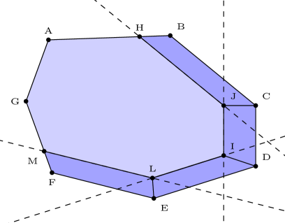
Figure 1.

We claim that we can apply Lemma 4.4 with $P$ replaced by $C_{a}(t,s)$ and $W(t)$ replaced by $N_{a}(t)$. For this to be the case, we need to know that the ‘side faces’ of $C_{a}(t,s)$ do not vary as $t$ is varied. Now a typical side facet is either the intersection of $C_{a}(t,s)$ with an old boundary facet $F$ of $\partial P^{+}$ or else the intersection $Z_{ab}(t,s)$ with $C_{b}(t,s)$ for some $b\neq a$. It is clear that $F$ does not move with $t$. As for $Z_{ab}(t,s)$, any point $x$ on it satisfies $\Phi_{a}(x)=\Phi_{b}(x)=t^{\prime}$, for $t\leqslant t^{\prime}\leqslant s$. In particular, the hyperplane containing the facet $Z_{ab}(t,s)$ is given by $\Phi_{b}(x)-\Phi_{a}(x)=0$ and its inward conormal is ${\mathrm{d}}\Phi_{b}-{\mathrm{d}}\Phi_{a}$. So such a facet also does not move with $t$.

Thus we can apply Lemma 4.4 to obtain

$$\int_{N_{a}(t)}\mbox{div}(\xi)\,{\mathrm{d}}\sigma_{a}= \frac{{\mathrm{d}}}{{\mathrm{d}}t}\int_{N_{a}(t)}\langle\xi,{\mathrm{d}}\Phi_{a}\rangle\,{\mathrm{d}}\sigma_{a}-\int_{\partial N_{a}(t)\cap\partial P_{t}^{+}}\langle\xi,\nu\rangle\,{\mathrm{d}}\tau$$ (5.13)

$$-\sum_{b}\int_{N_{a}(t)\cap N_{b}(t)}\langle\xi,{\mathrm{d}}(\Phi_{b}-{\mathrm{d}}\Phi_{a}\rangle\,{\mathrm{d}}\tau_{ab}$$ (5.14)

for any smooth vector field $\xi$ on $P$.

In the particular case that $\xi=fG{\mathrm{d}}\Phi_{a}$, the integral over $\partial N_{a}(t)\cap\partial P_{t}^{+}$ vanishes for the usual reason that $G\nu=0$ on any facet of $\partial P^{+}$ with conormal $\nu$ (cf. (3.3)). Thus we obtain

$$\int_{N_{a}(t)}\mbox{div}(fG{\mathrm{d}}\Phi_{a})\,{\mathrm{d}}\sigma_{a}=\frac{{\mathrm{d}}}{{\mathrm{d}}t}\int_{N_{a}(t)}|{\mathrm{d}}\Phi_{a}|^{2}_{g}\,{\mathrm{d}}\sigma_{a}-\sum_{b}\int_{N_{a}(t)\cap N_{b}(t)}\langle f\langle{\mathrm{d}}\Phi_{a},{\mathrm{d}}(\Phi_{b}-\Phi_{a})\rangle_{g}\,{\mathrm{d}}\tau_{ab}.$$ (5.15)

Summing over $a$, we get the formula

$$\int_{N(t)}\mbox{div}(fG{\mathrm{d}}\Phi)\,{\mathrm{d}}\sigma=\frac{{\mathrm{d}}}{{\mathrm{d}}t}\int_{N(t)}|{\mathrm{d}}\Phi|^{2}_{g}\,{\mathrm{d}}\sigma+\sum_{a<b}\int_{N_{a}(t)\cap N_{b}(t)}f|{\mathrm{d}}(\Phi_{b}-\Phi_{a})|^{2}_{g}\,{\mathrm{d}}\tau_{ab}.$$ (5.16)

The last term on the RHS here is $\int_{N(t)}f\,{\mathrm{d}}p$ by definition, so by combining this equation with (5.10), we obtain

$$\int_{P(t)}\partial_{i}\partial_{j}(fG^{ij})\,{\mathrm{d}}x=-\frac{{\mathrm{d}}}{{\mathrm{d}}t}\int_{\partial P(t)}f|{\mathrm{d}}\Phi|^{2}_{g}\,{\mathrm{d}}\sigma-2\int_{\partial P_{l}}f\,{\mathrm{d}}\sigma-\int_{N(t)}f\,{\mathrm{d}}p.$$ (5.17)

Substitution of this into (4.25) gives

$$\langle\hat{\rho}_{tk},f\rangle=k^{n}\int_{P(t)}f\,{\mathrm{d}}x+\frac{1}{2}k^{n-1}\int_{P(t)}s\,{\mathrm{d}}x+\frac{1}{2}k^{n-1}\langle\hat{a}_{t},f\rangle+k^{n-2}E_{k}[f],$$ (5.18)

where

$$\langle\hat{a}_{t},f\rangle=\int_{N(t)}f\,{\mathrm{d}}\sigma-\frac{1}{2}\frac{{\mathrm{d}}}{{\mathrm{d}}t}\int_{N(t)}f|{\mathrm{d}}\Phi|^{2}_{g}\,{\mathrm{d}}\sigma-\int_{N(t)}f\,{\mathrm{d}}p$$ (5.19)

as required. ∎

Setting $f=1$, we obtain the analogue of Proposition 4.6 in this case:

Proposition 5.3.

Let $g$ be any (smooth) toric Kähler metric on $X$ and let $s=s(g)$ be the scalar curvature. Denote by ${\mathrm{d}}p_{t}$ the above measure. If $t$ is not a critical value of the family $\{P(t)\}$,

$$\operatorname{Vol}(\partial P(t)^{+})=\int_{P(t)}s-\frac{{\mathrm{d}}}{{\mathrm{d}}t}\int_{N(t)}|\nu_{t}|^{2}\,{\mathrm{d}}\sigma_{t}-\int_{N(t)}{\mathrm{d}}p_{t},$$ (5.20)

where $s$ is the scalar curvature and $\nu_{t}$ is the conormal to $N_{t}$.

5.2. Test configurations and K-stability

In [Don02], Donaldson proposed a definition of K-stability for polarized varieties $(X,L)$ and, in the toric case, related K-stability to boundedness properties of the Mabuchi energy. We shall not reproduce the exact definition here. The rough idea is to consider ‘degenerations’ of $(X,L)$ to a (possibly very singular) polarized variety $(X_{0},L_{0})$ with a $\mathbb{C}^{\times}$-action. In this situation one can define the Donaldson–Futaki invariant $F_{1}$ of $(X_{0},L_{0})$; then $(X,L)$ is K-stable if $F_{1}<0$ for all possible degenerations.

In the toric case, there is a subclass of toric degenerations which can be defined combinatorially as follows. Let the polarized toric variety $(X,L)$ correspond to the convex integral polytope $P$. Now, given the data of the previous section, define $\widetilde{\Phi}_{a}(x,t)=\Phi_{a}(x)-t$ and consider the polytope $\Gamma\subset\mathbb{R}^{n+1}$ (the last variable being $t$),

$$\Gamma=P\times[0,\infty)\cap\bigcap_{a}\{\widetilde{\Phi}(x,t)\geqslant 0\}.$$ (5.21)

It is convenient to augment the defining equations for $\Gamma$ by explicitly including $\widetilde{\Phi}_{0}(x,t)=t$ which defines the base $t=0$ of $\Gamma$.

We refer to any such $\Gamma$ as (the polytope corresponding to) a toric test configuration for $(X,L)$. We note that the ‘roof’ of $\Gamma$ (see Figure 2(a)) is a union of $n$-dimensional convex polytopes $\tilde{N}_{a}$. Then $X_{0}$ in this case is obtained by gluing together the toric varieties corresponding to the $\tilde{N}_{a}$ to obtain a singular variety.

By definition, a product configuration arises when $\Gamma$ is $P\times[0,\infty)$ cut off (possibly obliquely) by a single affine function $\widetilde{\Phi}(x,t)\geqslant 0$—see Figure 2(b). A product configuration is called trivial if the roof is horizontal, i.e. given by $P\times\{c\}$ for some $c>0$.

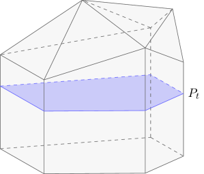
(a)

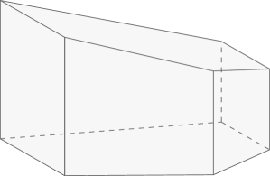
(b)

Figure 2.

In [Don02], the following combinatorial description of the Donaldson–Futaki invariant was given:

Proposition 5.4.

Let $(X,L)$ be a toric variety with moment polytope $P$ and let $\Gamma$ be a polytope defining a toric test configuration for $(X,L)$. Then the Donaldson–Futaki invariant of $\Gamma$ is the coefficient of $k^{-1}$ in the asymptotic expansion of $w_{k}/kd_{k}$, where

$$w_{k}=N(k\Gamma)-N(kP),\;\;d_{k}=N(kP)$$ (5.22)

and $N(A)$ denotes the number of lattice points in the integral polytope $A$.

The significance of this definition in relation to K-stability is as follows:

Definition 5.5.

Let $(X,L)$ be a toric variety with moment polytope $P$. We say that $(X,L)$ is K-polystable with respect to toric test configurations if for every toric test configuration corresponding to an $(n+1)$-dimensional polytope $\Gamma$ as above, the Donaldson–Futaki invariant $F_{1}$ is $\leqslant 0$, with equality if and only if $\Gamma$ corresponds to a product test configuration.

The reader is referred to [Don02, §4.2] for the details.

Our next theorem gives a formula for the Donaldson–Futaki invariant, given a choice of toric Kähler metric $g$, which is very analogous to the formula for the slope given in Theorem 1.3.

Clearly $\Gamma$ is closely related to the family $P_{t}$ of polytopes (5.1). More precisely, let $\pi$ denote the restriction to $\Gamma$ of the projection $(x,t)\mapsto t$. Then $\pi^{-1}(t)=P_{t}$, where $P_{t}$ is as in (5.1). By analogy with §5.1, let us introduce the following notation:

• Write $\partial\Gamma=\tilde{N}\cup\partial\Gamma^{+}$, where $N$ is the ‘roof’ of $\Gamma$, that is the union of the facets defined by the hyperplanes $\widetilde{\Phi}_{a}(x,t)=0$ and $\Gamma^{+}$ is the ‘vertical part’ of $\partial\Gamma$—the union of facets contained in sets of the form $F\times\mathbb{R}$, where $F$ is a facet of $P$.

• Define a positive measure ${\mathrm{d}}\tilde{p}$ with support on the $(n-1)$-skeleton of $\tilde{N}$ as follows: if $\tilde{N}_{ab}=\Gamma\cap\{\widetilde{\Phi}_{a}=0\}\cap\{\widetilde{\Phi}_{b}=0\}$, define

  $${\mathrm{d}}\tilde{p}_{ab}=|{\mathrm{d}}\widetilde{\Phi}_{a}-{\mathrm{d}}\widetilde{\Phi}_{b}|^{2}_{g}\,{\mathrm{d}}\tilde{\tau}_{ab}\mbox{ on the interior of }\widetilde{N}_{ab}.$$ (5.23)

  This makes sense because ${\mathrm{d}}\widetilde{\Phi}_{a}-{\mathrm{d}}\widetilde{\Phi}_{b}={\mathrm{d}}\Phi_{a}-{\mathrm{d}}\Phi_{b}$ is a $1$-form on $P$; its length can thus be measured with the toric metric $g$. Then define ${\mathrm{d}}\tilde{p}$ on $\tilde{N}$ to be equal to ${\mathrm{d}}\tilde{p}_{ab}$ on the relative interior of $\tilde{N}_{ab}$ for all $a\neq b$.

• We say that $c$ is a critical value of $\pi$ if $\pi^{-1}(c)$ contains a vertex of $\Gamma$. It is easily seen that $c$ is a critical value of $\pi$ if and only if it is one of the $c_{j}$ of (5.3).

Now define

$$\Delta(\Gamma)=\frac{1}{\operatorname{Vol}(\Gamma)}\int_{\widetilde{N}}{\mathrm{d}}\widetilde{p},$$ (5.24)

the integral being over the roof $\widetilde{N}$ of $\Gamma$. Since ${\mathrm{d}}\widetilde{p}$ is a non-negative measure,

$$\Delta(\Gamma)\geqslant 0\mbox{ for any }\Gamma$$ (5.25)

and

$$\Delta(\Gamma)=0\mbox{ if and only if the roof of $\Gamma$ has no codimension-2 faces}.$$ (5.26)

In other words, $\Delta(\Gamma)\geqslant 0$ with equality if and only if $\Gamma$ corresponds to a product test configuration.

Theorem 5.6.

Let $(X,L)$ be a smooth polarized toric variety with moment polytope $P\subset\mathbb{R}^{n}$. Let $\Gamma\subset\mathbb{R}^{n+1}$ be a polytope defining a toric test configuration for $(X,L)$. Then, for any choice of toric Kähler metric $g$ in the Kähler class $c_{1}(L)$ on $X$, the Donaldson–Futaki invariant of $\Gamma$ is given by

$$F_{1}=\frac{\operatorname{Vol}(\Gamma)}{2\operatorname{Vol}(P)}\left(\operatorname{Av}_{\Gamma}(\operatorname{pr}_{1}^{*}(s(g))-\operatorname{Av}_{P}(s(g))-\Delta(\Gamma)\right),$$ (5.27)

where $s(g)$ is the scalar curvature of $g$, $\operatorname{Av}_{A}(f)$ denotes average value of the function $f$ over the set $A$ and $\operatorname{pr}_{1}$ denotes the vertical projection $\Gamma\to P$.

The following is a simple consequence of (5.27):

Corollary 5.7 (cf. [ZZ08]).

Suppose that $X$ admits a toric cscK metric in the Kähler class $c_{1}(L)$. Then the Donaldson–Futaki invariant of any toric test configuration with polytope $\Gamma$ is $\leqslant 0$, with equality if and only if $\Gamma$ is a product configuration. In other words the existence of a toric cscK metric implies that $(X,L)$ is K-polystable with respect to toric test configurations.

Remark 7.

We follow the sign convention of [Don02] rather than [RT06] here, so for us negative Donaldson–Futaki invariant corresponds to stability.

Proof.

(Of the corollary.) If the scalar curvature $s$ is constant, then it is equal to its average over $P$ and also to the average of $\operatorname{pr}_{1}^{*}(s)$ over $\Gamma$. Thus these averages cancel from (5.27), leaving

$$F=-\frac{\operatorname{Vol}(\Gamma)}{2\operatorname{Vol}(P)}\Delta(\Gamma).$$

The result now follows from (5.25) and (5.26). ∎

5.3. Computation of the Donaldson–Futaki invariant

We use the following observation:

Lemma 5.8 ([Don02]).

The large-$k$ expansion of $w_{k}$ is given by

$$w_{k}=\operatorname{Vol}(\Gamma)k^{n+1}+\frac{1}{2}\operatorname{Vol}(\partial\Gamma^{+})k^{n}+O(k^{n-1}).$$ (5.28)

Given this result, the main problem is to understand $\operatorname{Vol}(\partial\Gamma^{+})$ in terms related to the metric. Since the intersection of $\partial\Gamma_{+}$ with a horizontal slice $P_{t}$ is the ‘old part’ $\partial P_{+}$ of the boundary of $P_{t}$, we have

$$\operatorname{Vol}(\partial\Gamma^{+})=\int_{0}^{c_{m}}\operatorname{Vol}(\partial P(t)^{+})\,{\mathrm{d}}t.$$ (5.29)

where $c_{m}$ is the largest critical value of $\pi$ as in (5.3). Combining this with Proposition 5.3, we shall obtain the formula:

Proposition 5.9.

With the above definitions and notation, we have

$$\operatorname{Vol}(\partial\Gamma^{+})=\int_{\Gamma}\operatorname{pr}_{1}^{*}(s)-\operatorname{Vol}(\Gamma)\Delta(\Gamma),$$ (5.30)

where $\operatorname{pr}_{1}$ is the restriction to $\Gamma$ of the projection $(x,t)\mapsto x$.

Proof.

We integrate (5.20) over each interval $(c_{j-1},c_{j})$ and sum over $j$, getting

$$\operatorname{Vol}(\partial\Gamma^{+}) =\int_{\Gamma}\operatorname{pr}_{1}^{*}(s)+\int_{N(0)}|\nu|^{2}\,{\mathrm{d}}\sigma-\sum_{j=1}^{m-1}\left(\int_{N(t_{j}^{-})}|\nu|^{2}\,{\mathrm{d}}\sigma-\int_{N(t_{j}^{+})}|\nu|^{2}\,{\mathrm{d}}\sigma\right)$$

$$-\int_{N(t_{m}^{-})}|\nu|^{2}\,{\mathrm{d}}\sigma-\int_{0}^{t_{m}}{\mathrm{d}}p_{t}\,{\mathrm{d}}t.$$ (5.31)

Now the integral over $N_{0}$ is zero because—by definition—$N_{0}$ is empty. Thus we have

$$\operatorname{Vol}(\partial\Gamma^{+})-\int_{\Gamma}\operatorname{pr}_{1}^{*}(s)=-\sum_{j=1}^{m-1}\left(\int_{N(t_{j}^{-})}|\nu|^{2}\,{\mathrm{d}}\sigma-\int_{N(t_{j}^{+})}|\nu|^{2}\,{\mathrm{d}}\sigma\right)-\int_{N(t_{m}^{-})}|\nu|^{2}\,{\mathrm{d}}\sigma-\int_{0}^{t_{m}}{\mathrm{d}}p_{t}\,{\mathrm{d}}t.$$ (5.32)

The next lemma matches up the terms on the RHS of this equation with the terms in the sum defining $\Delta(\Gamma)$, cf. (5.24). Recall that the roof $\tilde{N}$ of $\Gamma$ is a union of facets $\tilde{N}_{a}$ and its $(n-1)$-skeleton consists of intersections of the form $\tilde{N}_{ab}=\tilde{N}_{a}\cap\tilde{N}_{b}$. We call $\tilde{N}_{ab}$ horizontal if it is contained in a horizontal slice $P_{t}$ and non-horizontal otherwise. The point is that if $\tilde{N}_{ab}$ is horizontal, then it has to appear as a facet contained in $N(t)\subset\partial P(t)$ and moreover $t$ has to be a critical value of $\pi$, since $\tilde{N}_{ab}\subset\partial P_{t}$ certainly implies that $P_{t}$ contains a vertex of $\Gamma$. On the other hand, if $\tilde{N}_{ab}$ is not horizontal, then it meets $P_{t}$ non-trivially for $t$ in some interval $I$, and for each $t$ in the interior of $I$, $P_{t}\cap\tilde{N}_{ab}=N_{ab}(t)$ is part of the $(n-2)$-skeleton of $N(t)$. These rather simple observations may nonetheless help with the following:

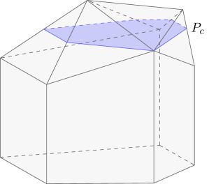
(a) A critical slice $P_{c}$ in the case where ${\mathrm{d}}\sigma_{t}$ and $\nu_{t}$ vary continuously through $t=c$.

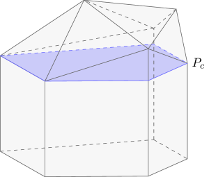
(b) A critical slice $P_{c}$ in the case where ${\mathrm{d}}\sigma_{t}$ and $\nu_{t}$ do not vary continuously through $t=c$.

Figure 3.

Lemma 5.10.

We have

$$\sum_{j=1}^{m-1}\left(\int_{N(c_{j}^{-})}|{\mathrm{d}}\Phi|_{g}^{2}\,{\mathrm{d}}\sigma-\int_{N(c_{j}^{+})}|{\mathrm{d}}\Phi|_{g}^{2}\,{\mathrm{d}}\sigma\right)+\int_{N(c_{m}^{-})}|{\mathrm{d}}\Phi|_{g}^{2}\,{\mathrm{d}}\sigma=\sum_{\tilde{N}_{ab}\,\mathrm{horizontal}}\int_{\tilde{N}_{ab}}{\mathrm{d}}\tilde{p}_{ab}.$$ (5.33)

and

$$\int_{0}^{c_{m}}{\mathrm{d}}p_{t}\,{\mathrm{d}}t=\sum_{\tilde{N}_{ab}\,\mathrm{not\,horizontal}}\int_{\tilde{N}_{ab}}{\mathrm{d}}\tilde{p}_{ab}.$$ (5.34)

Proof.

(See Fig. 3). Pick $c_{j}<c_{m}$, consider any facet $F$, say, of $P_{c_{j}}$ and in particular the contribution $F$ makes to the sum on the LHS of (5.33). Suppose first that $F$ is the intersection of $P_{c_{j}}$ with a single facet $\tilde{N}_{a}$ of $\Gamma$. Then $F_{t}=\tilde{N}_{a}\cap P_{t}$ for $t$ near $c_{j}$. Hence the Leray form and conormal of $F_{t}$ vary continously for $t$ near $c_{j}$. So such facets contribute nothing to the sum on the LHS of (5.33).

The other case to consider is that $F=\tilde{N}_{a}\cap\tilde{N}_{b}$. Note that this is necessarily a horizontal face of $\tilde{N}$. Suppose that $a$ and $b$ are ordered so that $F_{t}=P_{t}\cap\tilde{N}_{a}$ for $t<c_{j}$ but $F_{t}=P_{t}\cap\tilde{N}_{b}$ for $t>c_{j}$ (it always being assumed that $|t-c_{j}|$ is small). Then the contribution to the sum on the LHS of (5.33) is

$$\int_{F}(|{\mathrm{d}}\Phi_{a}|_{g}^{2}\,{\mathrm{d}}\sigma_{a}-|{\mathrm{d}}\Phi_{b}|_{g}^{2}\,{\mathrm{d}}\sigma_{b}).$$ (5.35)

We claim that this is equal to

$$\int_{\tilde{N}_{a}\cap\tilde{N}_{b}}|\widetilde{\Phi}_{a}-\widetilde{\Phi}_{b}|_{g}^{2}\,{\mathrm{d}}\tilde{\tau}_{ab}=\int_{\widetilde{N}_{ab}}{\mathrm{d}}\tilde{p}_{ab}.$$ (5.36)

Because $\tilde{N}_{a}$ and $\tilde{N}_{b}$ meet in a horizontal plane, we can choose affine coordinates on $\mathbb{R}^{n}$ so that

$$\widetilde{\Phi}_{a}(x,t)=Ax_{1}-t,\;\;\widetilde{\Phi}_{b}(x,t)=Bx_{1}-t,\mbox{ with }A>B>0.$$ (5.37)

(Thus $\Gamma$ is given locally by the intersection of the half-spaces $Ax_{1}\geqslant t$ and $Bx_{1}\geqslant t$.) Then

$${\mathrm{d}}\Phi_{a}=-A{\mathrm{d}}x_{1},{\mathrm{d}}\Phi_{b}=-B{\mathrm{d}}x_{1},\;\;{\mathrm{d}}\sigma_{a}=\frac{1}{A}{\mathrm{d}}x_{2}\ldots{\mathrm{d}}x_{n},{\mathrm{d}}\sigma_{b}=\frac{1}{B}{\mathrm{d}}x_{2}\ldots{\mathrm{d}}x_{n},$$ (5.38)

and so the integrand in (5.35) is

$$(A-B)|{\mathrm{d}}x_{1}|_{g}^{2}\,{\mathrm{d}}x_{2}\ldots{\mathrm{d}}x_{n}.$$ (5.39)

On the other hand,

$$|{\mathrm{d}}\widetilde{\Phi}_{a}-{\mathrm{d}}\widetilde{\Phi}_{b}|^{2}=(A-B)^{2}|{\mathrm{d}}x_{1}|^{2}_{g},\;\;{\mathrm{d}}\tilde{\tau}_{ab}=\frac{1}{A-B}{\mathrm{d}}x_{2}\ldots{\mathrm{d}}x_{n},$$ (5.40)

from which the equality of (5.35) and (5.36) follows.

This proves (5.33) except that we have ignored the last term on the LHS and the codimension-2 faces of $\Gamma$ contained in $t=t_{m}$. The required equality can be obtained by straightforward modification of the above discussion and further details are omitted. ∎

The proof of Proposition 5.9 follows by combining this Lemma with the definition of $\Delta(\Gamma)$. ∎

We can now easily complete the proof of Theorem 5.6: just substitute (5.30) into (5.28) and use

$$kd_{k}=\operatorname{Vol}(P)k^{n+1}\left(1+\frac{1}{2}\operatorname{Av}_{P}(s)k^{-1}+O(k^{-2})\right)$$ (5.41)

to calculate

$$\frac{w_{k}}{kd_{k}}=\frac{\operatorname{Vol}(\Gamma)}{\operatorname{Vol}(P)}+\frac{\operatorname{Vol}(\Gamma)}{2\operatorname{Vol}(P)}\left(\operatorname{Av}_{\Gamma}(\operatorname{pr}_{1}^{*}(s))-\operatorname{Av}_{P}(s)-\Delta(\Gamma)\right)k^{-1}+O(k^{-2}).$$

The result now follows from the definition of $F_{1}$ as the coefficient of $k^{-1}$ in $w_{k}/kd_{k}$.

References

- [Abr98] M. Abreu, Kähler geometry of toric varieties and extremal metrics, Internat. J. Math. 9 (1998), no. 6, 641–651.
- [Abr03] by same author, Kähler geometry of toric manifolds in symplectic coordinates, Symplectic and contact topology: interactions and perspectives (Toronto, ON/Montreal, QC, 2001), Fields Inst. Commun., vol. 35, Amer. Math. Soc., Providence, RI, 2003, pp. 1–24.
- [BBS08] R. Berman, B. Berndtsson, and J. Sjöstrand, A direct approach to Bergman kernel asymptotics for positive line bundles, Ark. Mat. 46 (2008), no. 2, 197–217.
- [Ber09] R. Berman, Bergman kernels and equilibrium measures for line bundles over projective manifolds, Amer. J. Math. 131 (2009), no. 5, 1485–1524.
- [BGU10] D. Burns, V. Guillemin, and A. Uribe, The spectral density function of a toric variety, Pure Appl. Math. Q. 6 (2010), no. 2, Special Issue: In honor of Michael Atiyah and Isadore Singer, 361–382.
- [Biq06] O. Biquard, Métriques kählériennes à courbure scalaire constante: unicité, stabilité, Astérisque (2006), no. 307, Exp. No. 938, vii, 1–31, Séminaire Bourbaki. Vol. 2004/2005. MR 2296414 (2008a:32023)
- [Cat99] D. Catlin, The Bergman kernel and a theorem of Tian, Analysis and geometry in several complex variables (Katata, 1997), Trends Math., Birkhäuser Boston, Boston, MA, 1999, pp. 1–23.
- [CDS12a] X.-X. Chen, S. Donaldson, and S. Sun, Kahler–Einstein metrics and stability, ArXiv preprint arXiv:1210.7494 (2012).
- [CDS12b] by same author, Kahler–einstein metrics on fano manifolds, i: approximation of metrics with cone singularities, ArXiv preprint arXiv:1211.4566 (2012).
- [CDS12c] by same author, Kahler–Einstein metrics on Fano manifolds, II: limits with cone angle less than , ArXiv preprint arXiv:1212.4714 (2012).
- [CDS13] by same author, Kahler–Einstein metrics on Fano manifolds, III: limits as the cone angle approaches and completion of the main proof, ArXiv preprint arXiv:1302.0282 (2013).
- [Don01] S. K. Donaldson, Scalar curvature and projective embeddings, I, J. Differential Geom. 59 (2001), no. 3, 479–522.
- [Don02] by same author, Scalar curvature and stability of toric varieties, J. Differential Geom. 62 (2002), no. 2, 289–349.
- [Don05a] by same author, Lower bounds on the Calabi functional, J. Differential Geom. 70 (2005), no. 3, 453–472. MR 2192937 (2006k:32045)
- [Don05b] by same author, Scalar curvature and projective embeddings. II, Q. J. Math. 56 (2005), no. 3, 345–356. MR 2161248 (2006f:32033)
- [Don09] by same author, Some numerical results in complex differential geometry, Pure Appl. Math. Q. 5 (2009), no. 2, Special Issue: In honor of Friedrich Hirzebruch. Part 1, 571–618. MR 2508897 (2010d:32020)
- [Fin10] J. Fine, Calabi flow and projective embeddings, J. Differential Geom. 84 (2010), no. 3, 489–523, With an appendix by Kefeng Liu and Xiaonan Ma. MR 2669363 (2012a:32023)
- [FKP+09] J. Fine, J. Keller, D. Panov, G. Szekelyhidi, and R. Thomas, Imperial College lunchtime working group on Bergman Kernels, private communication, 2009.
- [Ful93] W. Fulton, Introduction to toric varieties, Annals of Mathematics Studies, vol. 131, Princeton University Press, Princeton, NJ, 1993, The William H. Roever Lectures in Geometry.
- [GS07] V. Guillemin and S. Sternberg, Riemann sums over polytopes, Ann. Inst. Fourier (Grenoble) 57 (2007), no. 7, 2183–2195, Festival Yves Colin de Verdière.
- [Gui94] V. Guillemin, Kaehler structures on toric varieties, J. Differential Geom. 40 (1994), no. 2, 285–309.
- [KSW03] Y. Karshon, S. Sternberg, and J. Weitsman, Euler-maclaurin with remainder for a simple integral polytope, PNAS 100 (2003), no. 2, 426–433.
- [Lu00] Z. Lu, On the lower order terms of the asymptotic expansion of Tian-Yau-Zelditch, Amer. J. Math. 122 (2000), no. 2, 235–273.
- [MM07] X. Ma and G. Marinescu, Holomorphic Morse inequalities and Bergman kernels, Progress in Mathematics, vol. 254, Birkhäuser Verlag, Basel, 2007. MR 2339952 (2008g:32030)
- [Pok11] F. T. Pokorny, The Bergman Kernel on Toric Kähler Manifolds, Ph.D. thesis, University of Edinburgh, UK, 2011.
- [PS04] D. H. Phong and J. Sturm, Scalar curvature, moment maps, and the Deligne pairing, Amer. J. Math. 126 (2004), no. 3, 693–712. MR 2058389 (2005b:53137)
- [RT06] J. Ross and R. Thomas, An obstruction to the existence of constant scalar curvature Kähler metrics, J. Differential Geom. 72 (2006), no. 3, 429–466.
- [RT07] J. Ross and R. P. Thomas, A study of the Hilbert-Mumford criterion for the stability of projective varieties, J. Algebraic Geom. 16 (2007), no. 2, 201–255. MR 2274514 (2007k:14091)
- [SD10] R. Sena-Dias, Spectral measures on toric varieties and the asymptotic expansion of Tian-Yau-Zelditch, J. Symplectic Geom. 8 (2010), no. 2, 119–142.
- [Sto09] J. Stoppa, K-stability of constant scalar curvature Kähler manifolds, Adv. Math. 221 (2009), no. 4, 1397–1408. MR 2518643 (2010d:32024)
- [SZ04] B. Shiffman and S. Zelditch, Random polynomials with prescribed Newton polytope, J. Amer. Math. Soc. 17 (2004), no. 1, 49–108 (electronic). MR 2015330 (2005e:60032)
- [SZ07] J. Song and S. Zelditch, Convergence of Bergman geodesics on , Ann. Inst. Fourier (Grenoble) 57 (2007), no. 7, 2209–2237, Festival Yves Colin de Verdière. MR 2394541 (2009k:32025)
- [Tia90] G. Tian, On a set of polarized Kähler metrics on algebraic manifolds, J. Differential Geom 32 (1990), no. 1, 99–130.
- [Tia94] by same author, The -energy on hypersurfaces and stability, Comm. Anal. Geom. 2 (1994), no. 2, 239–265. MR 1312688 (95m:32030)
- [Tia97] by same author, Kähler-Einstein metrics with positive scalar curvature, Invent. Math. 130 (1997), no. 1, 1–37. MR 1471884 (99e:53065)
- [Tia12] by same author, K-stability and Kähler–Einstein metrics, ArXiv preprint arXiv:1211.4669 (2012).
- [Zel98] S. Zelditch, Szegő kernels and a theorem of Tian, Internat. Math. Res. Notices (1998), no. 6, 317–331.
- [ZZ08] B. Zhou and X. Zhu, -stability on toric manifolds, Proc. Amer. Math. Soc. 136 (2008), no. 9, 3301–3307. MR 2407096 (2010h:32030)