Distributed Signal Processing via Chebyshev Polynomial Approximation

Abstract

Unions of graph multiplier operators are an important class of linear operators for processing signals defined on graphs. We present a novel method to efficiently distribute the application of these operators. The proposed method features approximations of the graph multipliers by shifted Chebyshev polynomials, whose recurrence relations make them readily amenable to distributed computation. We demonstrate how the proposed method can be applied to distributed processing tasks such as smoothing, denoising, inverse filtering, and semi-supervised classification, and show that the communication requirements of the method scale gracefully with the size of the network.

I Introduction

In distributed signal processing tasks, the data to be processed is physically separated and cannot be transmitted to a central processing entity. This separation may be due to engineering limitations such as the limited communication range of wireless sensor network nodes, privacy concerns, or design considerations. Even when high-dimensional data can be processed centrally, it may be more efficient to process it with parallel computing. It is therefore important to develop distributed data processing algorithms that balance the trade-offs between performance, communication bandwidth, and computational complexity (speed).

I-A The Communication Network and Signals on the Network

For concreteness, we focus throughout the paper on distributed processing examples in wireless sensor networks; however, the problems we consider could arise in a number of different settings. Due to the limited communication range of wireless sensor nodes, each sensor node in a large network is likely to communicate with only a small number of other nodes in the network. To model the communication patterns, we can write down a graph with each vertex corresponding to a sensor node and each edge corresponding to a pair of nodes that communicate. Moreover, because the communication graph is a function of the distances between nodes, it often captures spatial correlations between sensors’ observations as well. That is, if two sensors are close enough to communicate, their observations are likely to be correlated. We can further specify these spatial correlations by adding weights to the edges of the graph, with higher weights associated to edges connecting sensors with closely correlated observations.

We model the communication network with an undirected, weighted graph ${\mathcal{G}}=\{{\mathcal{V}},{\mathcal{E}},w\}$, which consists of a set of vertices ${\mathcal{V}}$, a set of edges ${\mathcal{E}}$, and a weight function $w:{\mathcal{E}}\to\mathbb{R}^{+}$ that assigns a non-negative weight to each edge. We assume the number of nodes in the network, $N=|{\mathcal{V}}|$, is finite, and the graph is connected. The adjacency (or weight) matrix $\mathbf{W}$ for a weighted graph ${\mathcal{G}}$ is the $N\times N$ matrix with entries ${W}_{m,n}$, where

$${W}_{m,n}=\begin{cases}w(e),&\mbox{ if $e\in{\mathcal{E}}$ connects vertices $m$ and $n$}\\ 0,&\mbox{ otherwise}\end{cases}~{}.$$

Therefore, the weighted graph ${\mathcal{G}}$ can be equivalently represented as the triplet $\{{\mathcal{V}},{\mathcal{E}},\mathbf{W}\}$. The degree of each vertex is the sum of the weights of all the edges incident to it. We define the degree matrix $\mathbf{D}$ to be the diagonal matrix with the $n$th diagonal entry ${D}_{n,n}$ equal to the sum of the entries in the $n^{\mathrm{th}}$ row of $\mathbf{W}$.

A signal or function $f:{\mathcal{V}}\rightarrow\mathbb{R}$ defined on the vertices of the graph may be represented as a vector $\mathbf{f}\in\mathbb{R}^{N}$, where the $n^{\mathrm{th}}$ component of the vector $\mathbf{f}$ represents the function value at the $n^{\mathrm{th}}$ vertex in ${\mathcal{V}}$. Throughout, we use bold font to denote matrices and vectors, and we denote the $n^{\mathrm{th}}$ component of a vector $\mathbf{f}$ by either $f(n)$ or $f_{n}$.

I-B Distributed Signal Processing Tasks

We consider sensor networks whose nodes can only send messages to their local neighbors (i.e., they cannot communicate directly with a central entity). Much of the literature on distributed signal processing in such settings (see, e.g., [1]-[5] and references therein) focuses on coming to an agreement on simple features of the observed signal (e.g., consensus averaging, parameter estimation). We are more interested in processing the full function in a distributed manner, with each node having its own objective. Some example tasks under this umbrella include:

• Distributed denoising – In a sensor network of $N$ sensors, a noisy $N$-dimensional signal is observed, with each component of the signal corresponding to the observation at one sensor location. Using the prior knowledge that the denoised signal should be smooth or piecewise smooth with respect to the underlying weighted graph structure, the sensors’ task is to denoise each of their components of the signal by iteratively passing messages to their local neighbors and performing computations.

• Distributed semi-supervised learning / transductive classification – A class label is associated with each sensor node; however, only a small number of nodes in the network have knowledge of their labels. The cooperative task is for each node to learn its label by iteratively passing messages to its local neighbors and performing computations.

I-C Related Work

The tasks mentioned in Section I-B as well as other similar tasks have been considered recently in centralized settings in the fields of machine learning and signal processing on graphs [6]. For example, [7]-[9] consider general regularization frameworks on weighted graphs; [10]-[17] present graph-based semi-supervised learning methods; and [18]-[21] consider regularization and filtering on weighted graphs for image and mesh processing. Spectral regularization methods for ill-posed inverse problems (see, e.g., [22] and references therein) are also closely related.

Also in a centralized setting, [23] shows that a truncated Chebyshev polynomial expansion efficiently approximates the application of a spectral graph wavelet transform. The truncated Chebyshev polynomial expansion technique is originally introduced in [24] in the context of approximately computing the product of a matrix function and a vector. In Section II, we discuss the connection between the graph multiplier operators we define and more general matrix functions.

In the distributed setting, reference [25] considers denoising via wavelet processing and [26] presents a denoising algorithm that projects the measured signal onto a low-dimensional subspace spanned by smooth functions. References [27]-[30] consider different distributed regression problems. Reference [31] extends the approach proposed in this paper by examining robustness to quantization noise. Segarra et al. [32, 33] approximate general linear transformations by what we define in Section II-A as graph multiplier operators. Infinite impulse response (IIR) graph spectral filters, which have recently been introduced in [34, 35], comprise another approach to many distributed graph signal processing tasks. These filters, which we discuss in more detail in Section V-D, can be written as the ratio of two polynomial functions.

I-D Main Contributions

In the the initial presentation of this work [36], we extend the Chebyshev polynomial approximation method to the general class of unions of graph Fourier multiplier operators, and show how the recurrence properties of the Chebyshev polynomials also enable distributed application of these operators. The communication requirements for distributed computation using this method scale gracefully with the number of sensors in the network (and, accordingly, the size of the signals).

Our main contributions in this paper are to i) generalize graph Fourier multiplier operators to graph multiplier operators (to be defined in detail in Section II); ii) show that the application of linear operators that are unions of graph multiplier operators is a key component of distributed signal processing tasks such as distributed smoothing, denoising, inverse filtering, and semi-supervised learning; iii) present a novel method to efficiently distribute the application of the graph multiplier operators to high-dimensional signals; iv) provide theoretical bounds on the approximation error incurred by the proposed method; and v) theoretically and numerically compare the proposed method to alternative distributed computation methods.

The remainder of the paper is as follows. In the next section, we provide some background from spectral graph theory and matrix function theory, and introduce graph multiplier operators. In Section III, we provide examples of distributed signal processing tasks that feature the application of graph multiplier operators. In Section IV, we introduce a method to efficiently approximate these operators in a distributed setting via shifted Chebyshev polynomials. We discuss alternative methods to perform these approximate distributed computations in Section V, and we theoretically and numerically compare these alternative methods. In Section VI, we show how these methods can also be used to perform distributed wavelet denoising with the lasso regularization problem. Section VII concludes the paper.

II Matrix Functions and Graph Multiplier Operators

In this section, we leverage notation from the theory of matrix functions to introduce a class of operators that we call graph multiplier operators. We also relate these operators to multiplier operators from classical Fourier analysis.

II-A Matrix Functions

Functions of matrices [37] appear throughout mathematics, science, and engineering. While functions of more general matrices can be defined via the Jordan canonical form (e.g., [37, Definition 1.2, p. 3]), we restrict our attention in this paper to the simpler case of functions of real symmetric positive semi-definite matrices. Such a matrix $\mathbf{P}\in\mathbb{R}^{N\times N}$ has a complete set of orthonormal eigenvectors $\left\{\mathbf{u}_{\ell}\right\}_{\ell=0,1,\ldots,N-1}$ and associated real, non-negative eigenvalues $\left\{\lambda_{\ell}\right\}_{\ell=0,1,\ldots,N-1}$ satisfying $\mathbf{P}\mathbf{u}_{\ell}=\lambda_{\ell}\mathbf{u}_{\ell}$. That is, $\mathbf{P}$ admits a spectral decomposition $\mathbf{P}=\mathbf{U}\boldsymbol{\Lambda}\mathbf{U}^{*}$, where $\mathbf{U}$ is the $N\times N$ matrix with the $(\ell+1)^{\mathrm{th}}$ column equal to the eigenvector $\mathbf{u}_{\ell}$, and $\boldsymbol{\Lambda}$ is the $N\times N$ diagonal matrix with the $(\ell+1)^{\mathrm{th}}$ diagonal element equal to $\lambda_{\ell}$. Without loss of generality, we assume the eigenvalues to be ordered as

$$0\leq\lambda_{0}\leq\lambda_{1}\leq...\leq\lambda_{N-1}:=\lambda_{\max}.$$

Given a function $g(\cdot)$ well-defined on the spectrum $\sigma(\mathbf{P}):=\{\lambda_{0},\lambda_{1},\ldots,\lambda_{\max}\}$, the corresponding matrix function $g(\mathbf{P})$ is defined (e.g., [37, p.3]) as

$$g(\mathbf{P}):=\mathbf{U}g(\boldsymbol{\Lambda})\mathbf{U}^{*}:=\mathbf{U}\left[\begin{array}[]{ccc}g(\lambda_{0})&&\mathbf{0}\\ &\ddots&\\ \mathbf{0}&&g(\lambda_{N-1})\end{array}\right]\mathbf{U}^{*}.$$ (4)

The class of operators that can be written as matrix functions of $\mathbf{P}$ can be equivalently characterized as follows.

Proposition 1

For a fixed real symmetric positive semi-definite matrix $\mathbf{P}$, the following are equivalent:

• $\mathbf{\Psi}=g(\mathbf{P})$ for some $g:\sigma(\mathbf{P})\rightarrow\mathbb{R}$.

• $\mathbf{\Psi}$ and $\mathbf{P}$ are simultaneously diagonalizable by a unitary matrix; i.e., there exists a unitary matrix $\mathbf{U}$ such that $\mathbf{U}^{*}\mathbf{\Psi}\mathbf{U}$ and $\mathbf{U}^{*}\mathbf{P}\mathbf{U}$ are both diagonal matrices.

• $\mathbf{\Psi}$ and $\mathbf{P}$ commute; i.e., $\mathbf{\Psi}\mathbf{P}=\mathbf{P}\mathbf{\Psi}$.

Proof:

(a) implies (b) because of the definition (4) of $g(\mathbf{P})$, and (b) implies (a) if we set $g(\lambda_{\ell})$ to the $(\ell+1)^{\mathrm{th}}$ diagonal element of $\mathbf{U}^{*}\mathbf{\Psi}\mathbf{U}$. The equivalence between (b) and (c) is shown in [38, Corollary 4.5.18]. ∎

II-B Graph Multiplier Operators

In the context of distributed signal processing tasks, we are particularly interested in functions of symmetric matrices whose sparsity pattern is consistent with the communication structure of the network.

Definition 1

$\mathbf{\Psi}$ is a graph multiplier operator with respect to the graph ${\mathcal{G}}$ if there exists a real symmetric positive semi-definite matrix $\mathbf{P}$ and a function $g:\sigma(\mathbf{P})\rightarrow\mathbb{R}$ such that

• $\mathbf{\Psi}=g(\mathbf{P})=\sum_{\ell=0}^{N-1}g(\lambda_{\ell})\mathbf{u}_{\ell}\mathbf{u}_{\ell}^{*}$, and

• $P_{i,j}=0$ if $W_{i,j}=0$ and $i\neq j$; i.e., $\mathbf{P}$ has the same sparsity pattern as the graph Laplacian ${\mathbf{\cal L}}$ of the graph ${\mathcal{G}}$.

In order for the distributed computational methods we introduce in Sections IV and V to be applicable to a wider range of applications, we can generalize slightly from graph multiplier operators to unions of graph multiplier operators. A union of graph multiplier operators is a linear operator $\mathbf{\Phi}:\mathbb{R}^{N}\rightarrow\mathbb{R}^{\eta N}$ ($\eta\in\{1,2,\ldots\}$) that can be written as

$$~{}\begin{array}[]{c}{\color[rgb]{0,0,1}N}\\ {\color[rgb]{0,0,1}\overbrace{~{}\hskip 14.45377pt~{}}}\end{array}\vspace{-3in}$$ (7)

$$\mathbf{\Phi}=\left[\begin{array}[]{c}g_{1}(\mathbf{P})\\ g_{2}(\mathbf{P})\\ \vdots\\ g_{\eta}(\mathbf{P})\end{array}\right]= \left[\begin{array}[]{c}\mathbf{\Psi}_{1}\\ \mathbf{\Psi}_{2}\\ \vdots\\ \mathbf{\Psi}_{\eta}\end{array}\right]{\color[rgb]{0,0,1}\left.\begin{array}[]{c}{}\hfil\\ {}\hfil\\ {}\hfil\\ {}\hfil\end{array}\right\}{\eta N}}~{}~{}.$$ (20)

The application of the operator $\mathbf{\Phi}$ to a function $\mathbf{f}$ can equivalently be written as

$$\left(\mathbf{\Phi f}\right)_{(j-1)N+n}=\sum_{\ell=0}^{N-1}g_{j}(\lambda_{\ell})\langle\mathbf{f},\mathbf{u}_{\ell}\rangle u_{\ell}(n),$$ (21)

$$\hskip 62.59596pt\hbox{for }j\in\{1,2,\ldots,\eta\},~{}n\in\{1,2,\ldots,N\}.$$

II-C Graph Fourier Multiplier Operators

When the matrix $\mathbf{P}$ in Definition 1 is the graph Laplacian ${\mathbf{\cal L}}$, we call $\mathbf{\Psi}$ a graph Fourier multiplier operator. The non-normalized graph Laplacian is the real symmetric matrix ${\mathbf{\cal L}}:=\mathbf{D}-\mathbf{W}$, the difference between the degree matrix and the weighted adjacency matrix (see, e.g., [39, 40], for introductions to spectral graph theory). Because this situation arises frequently, we briefly motivate this terminology and relate it to the analogous operators from the classical signal processing literature.

For a function $f$ defined on the real line, a Fourier multiplier operator or filter $\Psi$ reshapes the function’s frequencies through multiplication in the Fourier domain:

$$\widehat{\Psi f}(\omega)=g(\omega)\hat{f}(\omega),\hbox{ for every frequency }\omega.$$

Taking an inverse Fourier transform yields

$$\Psi f(x) ={\cal F}^{-1}\Bigl{(}g(\omega){\cal F}(f)(\omega)\Bigr{)}(x)$$ (22)

$$=\frac{1}{2\pi}\int\limits_{\mathbb{R}}g(\omega)\hat{f}(\omega)e^{i\omega x}~{}d\omega.$$

Denoting the eigenvectors of ${\mathbf{\cal L}}$ by $\left\{\boldsymbol{\chi}_{\ell}\right\}_{\ell=0,1,\ldots,N-1}$, we can extend this straightforwardly to functions defined on the vertices of a graph by replacing the Fourier transform and its inverse in (22) with the graph Fourier transform $\hat{f}(\ell):=\langle\mathbf{f},\boldsymbol{\chi_{\ell}}\rangle=\sum_{n=1}^{N}f(n)\chi^{*}_{\ell}(n)$, and its inverse $f(n)=\sum_{\ell=0}^{N-1}\hat{f}(\ell)\chi_{\ell}(n).$ Namely, a graph Fourier multiplier operator is a linear operator $\Psi:\mathbb{R}^{N}\rightarrow\mathbb{R}^{N}$ that can be written as

$$\mathbf{\Psi f}(n) ={\cal F}^{-1}\Bigl{(}g(\lambda_{\ell}){\cal F}(f)(\ell)\Bigr{)}(n)$$

$$=\sum\limits_{\ell=0}^{N-1}g(\lambda_{\ell})\hat{f}(\ell)\chi_{\ell}(n).$$ (23)

We refer to $g(\cdot)$ as the multiplier or graph spectral filter. Equivalently, borrowing the above notation from the theory of matrix functions [37], we can write

$$\mathbf{\Psi}=g({\mathbf{\cal L}})=\sum_{\ell=0}^{N-1}g(\lambda_{\ell})\boldsymbol{\chi}_{\ell}\boldsymbol{\chi}_{\ell}^{*}=\boldsymbol{\chi}g(\boldsymbol{\Lambda})\boldsymbol{\chi}^{*}.$$

A high-level intuition behind graph spectral filtering (II-C) is as follows. The eigenvectors corresponding to the lowest eigenvalues of the graph Laplacian are the “smoothest” in the sense that $\left|\chi_{\ell}(m)-\chi_{\ell}(n)\right|$ is small for neighboring vertices $m$ and $n$. The inverse graph Fourier transform provides a representation of a signal $\mathbf{f}$ as a superposition of the orthonormal set of eigenvectors of the graph Laplacian. The effect of the graph Fourier multiplier operator $\mathbf{\Psi}$ is to modify the contribution of each eigenvector. For example, applying a multiplier $g(\cdot)$ that is 1 for all $\lambda_{\ell}$ below some threshold, and 0 for all $\lambda_{\ell}$ above the threshold is equivalent to projecting the signal onto the eigenvectors of the graph Laplacian associated with the lowest eigenvalues. This is analogous to ideal lowpass filtering in the continuous domain. Section III contains further intuition about and examples of graph Fourier multiplier operators. For more properties of the graph Laplacian eigenvectors, see [6] and [41], and references therein.

III Illustrative Distributed Signal Processing Applications

In this section, we show that a number of distributed signal processing tasks can be solved as applications of graph multiplier operators or unions of graph multiplier operators.

III-A Denoising with Distributed Tikhonov Regularization

First, we consider the distributed denoising task discussed in Section I. We start with a noisy signal $\mathbf{y}\in{\mathbb{R}}^{N}$ that is defined on a graph of $N$ sensors and has been corrupted by uncorrelated additive Gaussian noise. Through an iterative process of local communication and computation, each sensor should end up with a denoised estimate of its component, $f_{n}^{0}$, of the true underlying signal, $\mathbf{f}^{0}$.

To solve this problem, we enforce a priori information that the target signal is smooth with respect to the underlying graph topology. To enforce the global smoothness prior, we consider the class of regularization terms $\mathbf{f}^{{\!\scriptscriptstyle\mathrm{T}}}{\mathbf{\cal L}}^{r}\mathbf{f}$ for $r\geq 1$. The resulting distributed regularization problem has the form

$$\operatorname*{argmin}_{\mathbf{f}}\frac{\tau}{2}\lVert\mathbf{f}-\mathbf{y}\rVert_{2}^{2}+\mathbf{f}^{{\!\scriptscriptstyle\mathrm{T}}}{\mathbf{\cal L}}^{r}\mathbf{f}.$$ (24)

Intuitively, the regularization term $\mathbf{f}^{{\!\scriptscriptstyle\mathrm{T}}}{\mathbf{\cal L}}^{r}\mathbf{f}$ is small when the signal $\mathbf{f}$ has similar values at neighboring vertices with large weights (i.e., it is smooth). For example, when $r=1$,

$$\mathbf{f}^{{\!\scriptscriptstyle\mathrm{T}}}{\mathbf{\cal L}}\mathbf{f}=\frac{1}{2}\sum_{n\in{\mathcal{V}}}\sum_{m\sim n}\mathbf{W}_{m,n}\bigl{(}f_{m}-f_{n}\bigr{)}^{2}.$$

The proof of the following proposition is included in the Appendix.

Proposition 2

The solution to (24) is given by $\mathbf{Ry}$, where $\mathbf{R}$ is a graph Fourier multiplier operator of the form (II-C), with multiplier $g(\lambda_{\ell})=\frac{\tau}{\tau+2\lambda_{\ell}^{r}}$ .

So, one way to do distributed denoising is to approximately compute ${\mathbf{R}}\mathbf{y}$ in a distributed manner. We discuss methods to do this in Sections IV and V, and numerical examples are included in Section IV-D and Section V-E.

III-B Distributed Smoothing

An application closely related to distributed denoising is distributed smoothing. Here, the graph Fourier multiplier is the heat kernel $g(\lambda_{\ell})=e^{-t\lambda_{\ell}}$. In other words, a signal $\mathbf{y}\in\mathbb{R}^{N}$ is smoothed by computing $\mathbf{H}_{t}y$, where $(\mathbf{H}_{t}\mathbf{y})(n):=\sum_{\ell=0}^{N-1}e^{-t\lambda_{\ell}}\hat{y}(\ell)\chi_{\ell}(n)$ for fixed $t$. In the context of a centralized image smoothing application, [20] discusses in detail the heat kernel and its relationship to classical Gaussian filtering. Similar to both the example at the end of Section II-C and distributed Tikhonov regularization, the main idea is that the multiplier $g(\lambda_{\ell})=e^{-t\lambda_{\ell}}$ acts as a lowpass filter that attenuates the higher frequency (less smooth) components of $\mathbf{y}$. The distributed smoothing problem is to compute $\mathbf{R}\mathbf{y}$, with $\mathbf{R}=\mathbf{H}_{t}=e^{-t{\mathbf{\cal L}}}$ and each vertex $n$ beginning with only its observation $y_{n}$.

III-C Distributed Inverse Filtering

Next, we consider the situation where node $n$ observes the $n^{\mathrm{th}}$ component of $\mathbf{y}=\mathbf{\Psi f}+\boldsymbol{\nu}$, where $\mathbf{\Psi}$ is a graph Fourier multiplier operator with multiplier $g_{{\Psi}}(\cdot)$, and $\boldsymbol{\nu}$ is uncorrelated Gaussian noise. The task of the network is to recover $\mathbf{f}$ by inverting the effect of the graph multiplier operator $\mathbf{\Psi}$. This is the distributed graph analog to the deblurring problem in imaging, which is discussed in [42, Chapter 7]. As discussed in [42, Chapter 7], trying to recover $\mathbf{f}$ by simply applying the inverse filter in the graph Fourier domain, i.e., setting

$$f_{*}(n) =\sum_{\ell=0}^{N-1}\left(\frac{1}{g_{{\Psi}}(\lambda_{\ell})}\right)\hat{y}(\ell)\chi_{\ell}(n)$$

$$=\sum_{\ell=0}^{N-1}\left(\hat{f}(\ell)+\frac{\hat{\nu}(\ell)}{g_{{\Psi}}(\lambda_{\ell})}\right)\chi_{\ell}(n)$$

$$=f(n)+\sum_{\ell=0}^{N-1}\left(\frac{\hat{\nu}(\ell)}{g_{{\Psi}}(\lambda_{\ell})}\right)\chi_{\ell}(n),$$ (25)

does not work well when $g_{{\Psi}}(\cdot)$ is zero (or close to zero) for high frequencies, because the summation in (III-C) blows up, dominating $f(n)$. Therefore, we again use the prior that the signal is smooth with respect to the underlying graph structure, and approximately solve the regularization problem

$$\operatorname*{argmin}_{\mathbf{f}}\frac{\tau}{2}\lVert\mathbf{y}-\mathbf{\Psi f}\rVert_{2}^{2}+\mathbf{f}^{{\!\scriptscriptstyle\mathrm{T}}}{\mathbf{\cal L}}^{r}\mathbf{f}$$ (26)

in a distributed manner.

Proposition 3

The solution to (26) is given by $\mathbf{Ry}$, where $\mathbf{R}$ is a graph Fourier multiplier operator with multiplier

$$h(\lambda_{\ell}) =\frac{\tau g_{{\Psi}}(\lambda_{\ell})}{\tau g_{{\Psi}}^{2}(\lambda_{\ell})+2\lambda_{\ell}^{r}}.$$

The proof of Proposition 3 is included in the Appendix.

III-D Distributed Semi-Supervised Classification

The goal of semi-supervised classification is to learn a mapping from the data points $X=\{x_{1},x_{2},\ldots,x_{N}\}$ to their corresponding labels $Y=\{y_{1},y_{2},\ldots,y_{N}\}$. The pairs $(x_{i},y_{i})$ are independently and identically sampled from a joint distribution $p(x,y)$ over the sample space ${\cal X}\times{\cal Y},$ where ${\cal Y}:=\{1,2,\ldots,\kappa\}$ is the space of $\kappa$ classes. The transductive classification problem is to use the full set of data points $X=\{x_{1},x_{2},\ldots,x_{N}\}$ and the labels $Y_{l}=\{y_{1},y_{2},\ldots,y_{l}\}$ associated with a small portion of the data ($l\ll N$) to predict the labels $Y_{u}=\{y_{l+1},y_{l+2},\ldots,y_{N}\}$ associated with the unlabeled data $X_{u}=\{x_{l+1},x_{l+2},\ldots,x_{N}\}$.

Many semi-supervised learning methods represent the data $X$ by an undirected, weighted graph, and then force the labels to be smooth with respect to the intrinsic structure of this graph. We show how a number of these centralized graph-based semi-supervised classification methods can be written as applications of graph multiplier operators. Throughout, we assume there is one data point at each node in the graph, and the nodes know the weights of the edges connecting them to their neighbors in the graph. For example, each data point could be at a different node in a sensor network, and the weights could be a function of the physical distance between the nodes.

For different choices of reproducing kernel Hilbert spaces (RKHS) ${\cal H}$, a number of centralized semi-supervised classification methods estimate the label of the $n^{\mathrm{th}}$ data point ($n\in\{l+1,\ldots,N\}$) by

$$\operatorname*{arg\,max}_{j\in\{1,2,\ldots,\kappa\}}F_{nj}^{\mathrm{opt}},\hbox{ where~{}~{}~{}~{}~{}~{}~{}~{}~{}~{}~{}~{}}$$ (27)

$$\mathbf{F}^{\mathrm{opt}}=\operatorname*{argmin}_{\mathbf{F}\in{\mathbb{R}}^{N\times\kappa}}\sum_{j=1}^{\kappa}\left\{\tau\lVert\mathbf{F}_{:,j}-\mathbf{Y}_{:,j}\rVert_{2}^{2}+\lVert\mathbf{F}_{:,j}\rVert_{\cal H}^{2}\right\}.$$ (28)

In (28), $\mathbf{A}_{:,j}$ denotes the $j^{\mathrm{th}}$ column of a matrix $\mathbf{A}$; $\mathbf{Y}$ is an ${N\times\kappa}$ matrix with entries

$$Y_{ij}=\begin{cases}1,&\mbox{if }i\in\{1,2,\ldots,l\}\mbox{ and the label for point }i\mbox{ is }j\\ 0,&\mbox{otherwise}\end{cases};$$

and for some symmetric positive semi-definite matrix $\mathbf{S}\in\mathbb{R}^{N\times N}$,

$$\lVert\mathbf{f}\rVert_{\cal H}^{2}=\langle\mathbf{f},\mathbf{f}\rangle_{{\cal H}}:=\langle\mathbf{f},\mathbf{S}\mathbf{f}\rangle=\mathbf{f}^{{\!\scriptscriptstyle\mathrm{T}}}\mathbf{S}\mathbf{f}.$$ (29)

Note that for any symmetric positive semi-definite matrix $\mathbf{S}$, ${\cal H}$ endowed with the inner product defined in (29) is in fact a RKHS on $\mathbf{S}\mathbb{R}^{N}$, and its kernel is $k(i,j)=\left(\mathbf{S}^{-1}\right)_{ij}$, where $\mathbf{S}^{-1}$ denotes the pseudoinverse if $\mathbf{S}$ is not invertible [7, Theorem 4].

The following graph-based centralized semi-supervised classification methods fall into this category.

• In Tikhonov regularization, $\mathbf{S}={\mathbf{\cal L}}^{r}$ (e.g., [12])

• Zhou et al. [13] take $\mathbf{S}={{\mathbf{\cal L}}^{r}_{\mathrm{norm}}}$, where ${\mathbf{\cal L}}_{\mathrm{norm}}:=\mathbf{D}^{-\frac{1}{2}}{\mathbf{\cal L}}\mathbf{D}^{-\frac{1}{2}}$

• Smola and Kondor [7] consider a variety of kernel methods, including a diffusion process with $\mathbf{S}=\left[\exp\left(\frac{-\beta^{2}}{2}{{\mathbf{\cal L}}_{\mathrm{norm}}}\right)\right]^{-1}$, an inverse cosine with $\mathbf{S}=\left[\cos\left(\frac{\pi}{4}{\mathbf{\cal L}}_{\mathrm{norm}}\right)\right]^{-1}$, and an $r$-step random walk with $\mathbf{S}=\left(\beta\mathbf{I}_{N}-{\mathbf{\cal L}}_{\mathrm{norm}}\right)^{-r}$, where $\beta\geq 2$ and $\mathbf{I}_{N}$ is the $N\times N$ identity matrix

• Ando and Zhang’s K-scaling method [16, 17] takes

  $$\mathbf{S}=(\gamma\mathbf{I}_{N}+\mathbf{D})^{-\frac{1}{2}}(\gamma\mathbf{I}_{N}+{\mathbf{\cal L}})(\gamma\mathbf{I}_{N}+\mathbf{D})^{-\frac{1}{2}},$$

  which reduces to ${\mathbf{\cal L}}_{\mathrm{norm}}$ when $\gamma=0$.

• Zhu et al. [15, Chapter 15] take the kernel approach a step further by solving a convex optimization problem to find a good $\mathbf{S}$

Before moving on to the distributed semi-supervised classification problem, we note that in all of the examples above, we can write $\mathbf{S}=h(\mathbf{P})$ for some $h(\cdot)$, where $\mathbf{P}$ is either the combinatorial graph Laplacian, the normalized graph Laplacian, or the matrix $\mathbf{S}$ used in the K-scaling method, all of which have the same sparsity pattern as ${\mathbf{\cal L}}$ and are easily computable from the weighted adjacency matrix.

Now, $\mathbf{F}^{\mathrm{opt}}$ in (28) can be equivalently rewritten as the solution to $\kappa$ separate minimization problems, with

$$\mathbf{F}_{:,j}^{\mathrm{opt}} =\operatorname*{argmin}_{\mathbf{f}\in{\mathbb{R}}^{N}}\left\{\tau\lVert\mathbf{f}-\mathbf{Y}_{:,j}\rVert_{2}^{2}+\mathbf{f}^{{\!\scriptscriptstyle\mathrm{T}}}\mathbf{S}\mathbf{f}\right\}$$

$$=\operatorname*{argmin}_{\mathbf{f}\in{\mathbb{R}}^{N}}\left\{\tau\lVert\mathbf{f}-\mathbf{Y}_{:,j}\rVert_{2}^{2}+\mathbf{f}^{{\!\scriptscriptstyle\mathrm{T}}}h(\mathbf{P})\mathbf{f}\right\}.$$ (30)

We can write the solution to (III-D) as $\mathbf{R}\mathbf{Y}_{:,j}$, where $\mathbf{R}$ is a graph multiplier operator of the form outlined in Definition 1, with respect to $\mathbf{P}$. The optimal multiplier is $g(\lambda_{\ell})=\frac{\tau}{\tau+h(\lambda_{\ell})}$.

Therefore, the following is a method to distribute any of the centralized semi-supervised classification methods that can be written as (27) and (28):

1. Node $n$ starts with or computes the entries of the $n^{\mathrm{th}}$ row of $\mathbf{P}$

2. Each node $n$ forms the $n^{\mathrm{th}}$ row of $\mathbf{Y}$

3. For every $j\in\{1,2,\ldots,\kappa\}$, the nodes approximately compute ${\mathbf{F}}^{\mathrm{opt}}_{:,j}:={\mathbf{R}}\mathbf{Y}_{:,j}$ in a distributed manner via algorithms outlined in the subsequent sections.

4. Each node $n$ with an unlabeled data point computes its label estimate according to $\operatorname*{arg\,max}_{j\in\{1,2,\ldots,\kappa\}}\left\{{F}_{nj}^{\mathrm{opt}}\right\}$

IV Distributed Chebyshev Polynomial Approximation of Graph Multiplier Operators

Motivated by the fact that a number of distributed signal processing tasks can be viewed as applications of unions of graph multiplier operators, we proceed to the issue of how to approximately compute $\mathbf{\Phi f}$, where $\mathbf{\Phi}$ is of the form (7), in a distributed setting. In this section, we introduce a computationally efficient approximation to unions of graph multiplier operators based on shifted Chebyshev polynomials.

IV-A The Centralized Chebyshev Polynomial Approximation

Exactly computing $g(\mathbf{P})\mathbf{f}$ requires explicit computation of the entire set of eigenvectors and eigenvalues of $\mathbf{P}$, which becomes computationally challenging as the size of the network, $N$, increases, even in a centralized setting. Druskin and Knizhnerman [24] introduce a method to approximate $g(\mathbf{P})\mathbf{f}$ by $\tilde{g}(\mathbf{P})\mathbf{f}$, where $\tilde{g}(\cdot)$ is a polynomial approximation of $g(\cdot)$ computed by truncating a shifted Chebyshev series expansion of the function $g(\cdot)$ on the interval $[\lambda_{\min},\lambda_{\max}]$. Doing so circumvents the need to compute the full set of eigenvectors and eigenvalues of $\mathbf{P}$. This idea is extended to unions of graph Fourier multipliers in [23, Section 6]; that is, a computationally efficient approximation $\tilde{\mathbf{\Phi}}\mathbf{f}$ of $\mathbf{\Phi f}$ can be computed by approximating each multiplier $g_{j}(\cdot)$ by a truncated series of shifted Chebyshev polynomials. We summarize this approach below.

For $y\in[-1,1]$, the Chebyshev polynomials $\left\{T_{k}(y)\right\}_{k=0,1,2,\ldots}$ are generated by

$$T_{k}(y):=\begin{cases}1,&\hbox{ if }k=0\\ y,&\hbox{ if }k=1\\ 2yT_{k-1}(y)-T_{k-2}(y),&\hbox{ if }k\geq 2\end{cases}.$$

These Chebyshev polynomials form an orthogonal basis for
$L^{2}\left([-1,1],\frac{dy}{\sqrt{1-y^{2}}}\right)$. So every function $h$ on $[-1,1]$ that is square integrable with respect to the measure $dy/\sqrt{1-y^{2}}$ can be represented as $h(y)=\frac{1}{2}b_{0}+\sum_{k=1}^{\infty}b_{k}T_{k}(y)$, where $\{b_{k}\}_{k=0,1,\ldots}$ is a sequence of Chebyshev coefficients that depends on $h(\cdot)$. For a detailed overview of Chebyshev polynomials, including the above definitions and properties, see [43]–[45].

By shifting the domain of the Chebyshev polynomials to $[0,\lambda_{\max}]$ via the transformation $x=\frac{\lambda_{\max}}{2}(y+1)$, we can represent each multiplier as

$$g_{j}(x)=\frac{1}{2}c_{j,0}+\sum_{k=1}^{\infty}c_{j,k}\overline{T}_{k}(x),\hbox{ for all }x\in[0,\lambda_{\max}],$$ (31)

where $\overline{T}_{k}(x):=T_{k}\left(\frac{x-\alpha}{\alpha}\right)$, $\alpha:=\frac{\lambda_{\max}}{2}$, and

$$c_{j,k}:=\frac{2}{\pi}\int_{0}^{\pi}\cos(k\phi)~{}g_{j}\Bigl{(}\alpha\bigl{(}\cos(\phi)+1\bigr{)}\Bigr{)}~{}d\phi.$$ (32)

For $k\geq 2$, the shifted Chebyshev polynomials satisfy

$$\overline{T}_{k}(x)=\frac{2}{\alpha}(x-\alpha)\overline{T}_{k-1}(x)-\overline{T}_{k-2}(x).$$

Thus, for any $\mathbf{f}\in{\mathbb{R}}^{N}$, we have

$$\overline{{T}}_{k}(\mathbf{P})\mathbf{f}=\frac{2}{\alpha}({\mathbf{P}}-{\alpha}\mathbf{I})\left(\overline{{T}}_{k-1}(\mathbf{P})\mathbf{f}\right)-\overline{{T}}_{k-2}(\mathbf{P})\mathbf{f},$$ (33)

where $\overline{{T}}_{k}(\mathbf{P})\in\mathbb{R}^{N\times N}$ and, by (21), the $n^{\mathrm{th}}$ element of $\overline{{T}}_{k}(\mathbf{P})\mathbf{f}$ is given by

$$\left(\overline{{T}}_{k}({P}){f}\right)_{n}=\sum_{\ell=0}^{N-1}\overline{T}_{k}(\lambda_{\ell})\langle\mathbf{f},\mathbf{u}_{\ell}\rangle u_{\ell}(n).$$ (34)

Now, to approximate the operator $\mathbf{\Phi}$, we can approximate each multiplier $g_{j}(\cdot)$ by the first $K+1$ terms in its Chebyshev polynomial expansion (31). Then, for every $j\in\{1,2,\ldots,\eta\}$ and $n\in\{1,2,\ldots,N\}$, we have

$$\left(\tilde{{\Phi}}{f}\right)_{(j-1)N+n}$$

$$\quad\quad:=\left(\frac{1}{2}c_{j,0}{f}+\sum_{k=1}^{K}c_{j,k}\overline{{T}}_{k}({P}){f}\right)_{n}$$ (35)

$$\quad\quad\stackrel{{\scriptstyle(\ref{Eq:T_bar_def})}}{{=}}\sum_{\ell=0}^{N-1}\left[\frac{1}{2}c_{j,0}+\sum_{k=1}^{K}c_{j,k}\overline{T}_{k}(\lambda_{\ell})\right]\langle\mathbf{f},\mathbf{u}_{\ell}\rangle u_{\ell}(n)$$

$$\quad~{}\quad\approx\sum_{\ell=0}^{N-1}\left[\frac{1}{2}c_{j,0}+\sum_{k=1}^{\infty}c_{j,k}\overline{T}_{k}(\lambda_{\ell})\right]\langle\mathbf{f},\mathbf{u}_{\ell}\rangle u_{\ell}(n)$$

$$\quad\quad\stackrel{{\scriptstyle(\ref{Eq:multiplier_expansion})}}{{=}}\sum_{\ell=0}^{N-1}g_{j}(\lambda_{\ell})\langle\mathbf{f},\mathbf{u}_{\ell}\rangle u_{\ell}(n)$$

$$\quad~{}\quad\stackrel{{\scriptstyle(\ref{Eq:operator_def})}}{{=}}\left({\Phi f}\right)_{(j-1)N+n}.$$

To recap, we propose to compute $\tilde{\mathbf{\Phi}}\mathbf{f}$ by first computing the Chebyshev coefficients $\{c_{j,k}\}_{j=1,2,\ldots,\eta;~{}k=1,2,\ldots,K}$ according to (32), and then computing the sum in (IV-A). The computational benefit of the Chebyshev polynomial approximation arises in (IV-A) from the fact the vector $\overline{{T}}_{k}(\mathbf{P})\mathbf{f}$ can be computed recursively from $\overline{{T}}_{k-1}(\mathbf{P})\mathbf{f}$ and $\overline{{T}}_{k-2}(\mathbf{P})\mathbf{f}$ according to (33). The computational cost of doing so is dominated by the cost of matrix-vector multiplication with $\mathbf{P}$, which is proportional to the number of edges, $|{\mathcal{E}}|$ [23]. Therefore, if the underlying communication graph is sparse (i.e., $|{\mathcal{E}}|$ scales linearly with the network size $N$), it is far more computationally efficient to compute $\tilde{\mathbf{\Phi}}\mathbf{f}$ than $\mathbf{\Phi f}$. Finally, we note that in practice, setting the approximation order $K$ to around 20 results in $\tilde{\mathbf{\Phi}}$ approximating $\mathbf{\Phi}$ closely enough for the applications we have examined.

IV-B Distributed Computation of $\tilde{\mathbf{\Phi}}\mathbf{f}$

We now discuss the second benefit of the Chebyshev polynomial approximation: it is easily distributable. We consider the following scenario. There is a network of $N$ nodes, and each node $n$ begins with the following knowledge:

• $f(n)$, the $n^{\mathrm{th}}$ component of the signal $\mathbf{f}$

• The identity of its neighbors, and the weights of the graph edges connecting itself to each of its neighbors

• The Chebyshev coefficients, $c_{j,k}$, for $j\in\{1,2,\ldots,\eta\}$ and $k\in\{0,1,2,\ldots,K\}$. These can either be computed centrally according to (32) and then transmitted throughout the network, or each node can begin with knowledge of the multipliers, $\{g_{j}(\cdot)\}_{j=1,2,\ldots,\eta}$, and precompute the Chebyshev coefficients according to (32)

• An upper bound $\overline{\lambda_{\max}}$ on $\lambda_{\max}$, the largest eigenvalue of $\mathbf{P}$. This bound need not be tight. For example, when $\mathbf{P}$ is the graph Laplacian ${\mathbf{\cal L}}$, we can precompute a bound such as $\lambda_{\max}\leq\max\{d(m)+d(n);m\sim n\}$, where $d(n)$ is the degree of node $n$ [46][47, Corollary 3.2]

The task is for each network node $n$ to compute

$$\Big{\{}\Big{(}\tilde{{\Phi}}{f}\Big{)}_{(j-1)N+n}\Big{\}}_{j=1,2,\ldots,\eta}$$ (36)

by iteratively exchanging messages with its local neighbors in the network and performing some computations.

As a result of (IV-A), for node $n$ to compute the desired sequence in (36), it suffices to learn $\left\{\left(\overline{{T}}_{k}({P}){f}\right)_{n}\right\}_{k=1,2,\ldots,K}$. Note that $\left(\overline{{T}}_{1}({{P}}){f}\right)_{n}=\left(\frac{1}{\alpha}({{P}}-{\alpha}{I}){f}\right)_{n}$ and $P_{n,m}=0$ for all nodes $m$ that are not neighbors of node $n$. Thus, to compute $\left(\overline{{T}}_{1}({{P}}){f}\right)_{n}$, node $n$ just needs to receive $f(m)$ from all neighbors $m$. So once all nodes send their component of the signal to their neighbors, they are able to compute their respective components of $\overline{{T}}_{1}({\mathbf{P}})\mathbf{f}$. In the next step, each node $n$ sends the newly computed quantity $\left(\overline{{T}}_{1}({{P}}){f}\right)_{n}$ to all of its neighbors, enabling the distributed computation of $\overline{{T}}_{2}({\mathbf{P}})\mathbf{f}$ according to (33). The iterative process of local communication and computation continues for $K$ rounds until each node $n$ has computed the required sequence $\left\{\left(\overline{{T}}_{k}({P}){f}\right)_{n}\right\}_{k=1,2,\ldots,K}$. In all, $2K\lvert{{\mathcal{E}}}\rvert$ messages of length 1 are required for every node $n$ to compute its sequence of coefficients in (36) in a distributed fashion. This distributed computation process is summarized in Algorithm 1.

Algorithm 1 Distributed Computation of $\tilde{\mathbf{\Phi}}\mathbf{f}$

Inputs at node $n$: $f_{n}$, $P_{n,m}~{}\forall m$, $\left\{c_{k,j}\right\}_{j=1,2,\ldots,\eta;~{}k=0,1,\ldots,K}$,
and $\overline{\lambda_{\max}}$
Outputs at node $n$: $\left\{\left(\tilde{\Phi}f\right)_{(j-1)N+n}\right\}_{j=1,2,\ldots,\eta}$

1:  Set $\alpha=\frac{\overline{\lambda_{\max}}}{2}$

2:  Set $\left(\overline{{T}}_{0}({P}){f}\right)_{n}=f_{n}$

3:  Transmit $f_{n}$ to all neighbors ${\cal N}_{n}:=\{m:P_{n,m}\neq 0\}$

4:  Receive $f_{m}$ from all neighbors ${\cal N}_{n}$

5:  Compute and store

$$\left(\overline{{T}}_{1}({P}){f}\right)_{n}=\sum\limits_{m\in{\cal N}_{n}\cup n}\frac{1}{\alpha}P_{n,m}f_{m}-f_{n}$$

6:  for $k=2,\ldots,K$ do

7:     Transmit $\left(\overline{{T}}_{k-1}({P}){f}\right)_{n}$ to all neighbors ${\cal N}_{n}$

8:     Receive $\left(\overline{{T}}_{k-1}({P}){f}\right)_{m}$ from all neighbors ${\cal N}_{n}$

9:     Compute and store

$$\left(\overline{{T}}_{k}({P}){f}\right)_{n}= \sum\limits_{m\in{\cal N}_{n}\cup n}\frac{2}{\alpha}P_{n,m}\left(\overline{{T}}_{k-1}({P}){f}\right)_{m}$$

$$-2\left(\overline{{T}}_{k-1}({P}){f}\right)_{n}-\left(\overline{{T}}_{k-2}({P}){f}\right)_{n}$$

10:  end for

11:  for $j\in\{1,2,\ldots,\eta\}$ do

12:     Output

$$\left(\tilde{{\Phi}}{f}\right)_{(j-1)N+n}=\frac{1}{2}c_{j,0}f_{n}+\sum\limits_{k=1}^{K}c_{j,k}\left(\overline{{T}}_{k}({P}){f}\right)_{n}$$

13:  end for

An important point to emphasize again is that although the operator $\mathbf{\Phi}$ and its approximation $\tilde{\mathbf{\Phi}}$ are defined through the eigenvectors of $\mathbf{P}$, the Chebyshev polynomial approximation helps the nodes apply the operator to the signal without explicitly computing (individually or collectively) the eigenvalues or eigenvectors of $\mathbf{P}$, other than the upper bound on its spectrum. Rather, they initially communicate their component of the signal to their neighbors, and then communicate simple weighted combinations of the messages received in the previous stage in subsequent iterations. In this way, information about each component of the signal $\mathbf{f}$ diffuses through the network without direct communication between non-neighboring nodes.

IV-C Distributed Computation of $\tilde{\mathbf{\Phi}}^{*}\mathbf{a}$ and $\tilde{\mathbf{\Phi}}^{*}\tilde{\mathbf{\Phi}}\mathbf{f}$

In some tasks, such as the distributed lasso presented in Section VI, we not only need to apply unions of graph multiplier operators, but we also need to apply their adjoints. The application of the adjoint $\tilde{\mathbf{\Phi}}^{*}$ of the Chebyshev polynomial approximate operator $\tilde{\mathbf{\Phi}}$ can also be computed in a distributed manner. Let $\mathbf{a}=\left[\mathbf{a}_{1};\mathbf{a}_{2};\ldots;\mathbf{a}_{\eta}\right]\in\mathbb{R}^{\eta N}$, where $\mathbf{a}_{j}\in\mathbb{R}^{N}$. Then it is straightforward to show that

$$\left(\tilde{{\Phi}}^{*}{a}\right)_{n}=\sum_{j=1}^{\eta}\left(\frac{1}{2}c_{j,0}{a}_{j}+\sum_{k=1}^{K}c_{j,k}\overline{{T}}_{k}(P){a}_{j}\right)_{n}.$$ (37)

We assume each node $n$ starts with knowledge of $a_{j}(n)$ for all $j\in\{1,2,\ldots,\eta\}$. For each $j\in\{1,2,\ldots,\eta\}$, the distributed computation of the corresponding term on the right-hand side of (37) is done in an analogous manner to the distributed computation of $\tilde{\mathbf{\Phi}}\mathbf{f}$ discussed above. Since this has to be done for each $j$, $2K|{\mathcal{E}}|$ messages, each a vector of length $\eta$, are required for every node $n$ to compute $(\tilde{{\Phi}}^{*}{a})_{n}$. The distributed computation of $\tilde{\mathbf{\Phi}}^{*}\mathbf{a}$ is summarized in Algorithm 2.

Algorithm 2 Distributed Computation of $\tilde{\mathbf{\Phi}}^{*}\mathbf{a}$

Inputs at node $n$: $\left\{a_{j}(n)\right\}_{j=1,2,\ldots,\eta}$, $P_{n,m}~{}\forall m$, $\overline{\lambda_{\max}}$,
and $\left\{c_{k,j}\right\}_{j=1,2,\ldots,\eta;~{}k=0,1,\ldots,K}$,
Output at node $n$: $\left(\tilde{{\Phi}}^{*}{a}\right)_{n}$

1:  Set $\alpha=\frac{\overline{\lambda_{\max}}}{2}$

2:  for $j=1,2,\ldots,\eta$ do

3:     Set $\left(\overline{{T}}_{0}(P){a}_{j}\right)_{n}=a_{j}(n)$

4:  end for

5:  Transmit $\left\{a_{j}(n)\right\}_{j=1,2,\ldots,\eta}$ to all neighbors ${\cal N}_{n}:=\{m:P_{n,m}\neq 0\}$

6:  Receive $\left\{a_{j}(m)\right\}_{j=1,2,\ldots,\eta}$ from all neighbors ${\cal N}_{n}$

7:  for $j=1,2,\ldots,\eta$ do

8:     Compute and store

$$\left(\overline{{T}}_{1}({\mathbf{\cal L}}){a}_{j}\right)_{n}=\sum\limits_{m\in{\cal N}_{n}\cup n}\frac{2}{\alpha}P_{n,m}a_{j}(m)-2a_{j}(n)$$

9:  end for

10:  for $k=2,\ldots,K$ do

11:     Transmit $\left\{\left(\overline{{T}}_{k-1}(P){a}_{j}\right)_{n}\right\}_{j=1,2,\ldots,\eta}$ to all neighbors ${\cal N}_{n}$

12:     Receive $\left\{\left(\overline{{T}}_{k-1}(P){a}_{j}\right)_{m}\right\}_{j=1,2,\ldots,\eta}$ from all neighbors ${\cal N}_{n}$

13:     for $j=1,2,\ldots,\eta$ do

14:        Compute and store

$$\left(\overline{{T}}_{k}(P){a}_{j}\right)_{n}= \sum\limits_{m\in{\cal N}_{n}\cup n}\frac{2}{\alpha}P_{n,m}\left(\overline{{T}}_{k-1}(P){a}_{j}\right)_{m}$$

$$-2\left(\overline{{T}}_{k-1}(P)\mathbf{a}_{j}\right)_{n}-\left(\overline{{T}}_{k-2}(P)\mathbf{a}_{j}\right)_{n}$$

15:     end for

16:  end for

17:  Output

$$\left(\tilde{{\Phi}}^{*}{a}\right)_{n}=\sum_{j=1}^{\eta}\left\{\frac{1}{2}c_{j,0}a_{j}(n)+\sum_{k=1}^{K}c_{j,k}\left(\overline{{T}}_{k}(P){a}_{j}\right)_{n}\right\}.$$

Using the property of the Chebyshev polynomials that $T_{k}(x)T_{k^{\prime}}(x)=\frac{1}{2}\left[T_{k+k^{\prime}}(x)+T_{|k-k^{\prime}|}(x)\right]$, we can write

$$\left(\tilde{{\Phi}}^{*}\tilde{{\Phi}}{f}\right)_{n}=\left(\frac{1}{2}d_{0}{f}+\sum_{k=1}^{2K}d_{k}\overline{{T}}_{k}(P){f}\right)_{n}.$$

See [23, Section 6.1] for a similar calculation and an explicit formula for the coefficients $\left\{d_{k}\right\}_{k=0,1,\ldots,2K}$. Thus, with each node $n$ starting with $f(n)$ as in Section IV-B, $\tilde{\mathbf{\Phi}}^{*}\tilde{\mathbf{\Phi}}\mathbf{f}$ can be distributedly computed using $4K|{\mathcal{E}}|$ messages of length 1, with each node $n$ finishing with knowledge of $\left(\tilde{{\Phi}}^{*}\tilde{{\Phi}}{f}\right)_{n}$.

IV-D Numerical Example

We place 500 sensors randomly in the $[0,1]\times[0,1]$ square. We then construct a weighted graph according to a thresholded Gaussian kernel weighting function based on the physical distance between nodes. The weight of edge $e$ connecting nodes $i$ and $j$ that are a distance $d(i,j)$ apart is

$$w(e)=\begin{cases}\exp\left({-\frac{[d(i,j)]^{2}}{2\theta^{2}}}\right)&\mbox{if }d(i,j)\leq\kappa\\ 0&\mbox{otherwise}\end{cases},$$

with parameters $\sigma=0.074$ and $\kappa=0.075$. We create a smooth 500-dimensional signal with the $n^{\mathrm{th}}$ component given by $h_{n}=n_{x}^{2}+n_{y}^{2}-1$, where $n_{x}$ and $n_{y}$ are node $n$’s $x$ and $y$ coordinates in $[0,1]\times[0,1]$. Next, we corrupt each component of the signal ${\bf h}$ with uncorrelated additive Gaussian noise with mean zero and standard deviation 0.5, resulting in a noisy signal ${\bf y}$. Then we apply the graph Fourier multiplier operator $\tilde{\bf R}$, the Chebyshev polynomial approximation to ${\bf R}$ from Proposition 2, with $\tau=r=1$ and $K=20$. The original signal ${\bf h}$, noisy signal ${\bf y}$, and denoised signal $\tilde{\mathbf{R}}\mathbf{y}$ are shown in Figure 1(a)-(c). The Chebyshev polynomial approximation errors are shown in Figure 1(d), and the resulting approximation errors for the graph Fourier multiplier operator and denoised signal are shown in Figure 1(e). We repeated this entire experiment 1000 times, with a new random graph and random noise each time, and the average mean square error for the denoised signals was 0.013, as compared to 0.250 average mean square error for the noisy signals.

Original

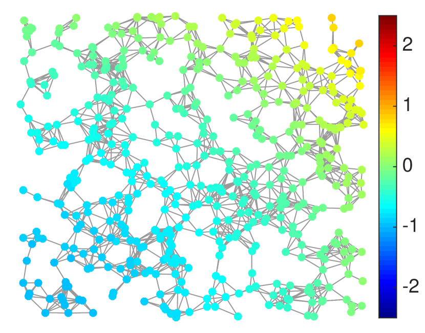
(a)

Noisy

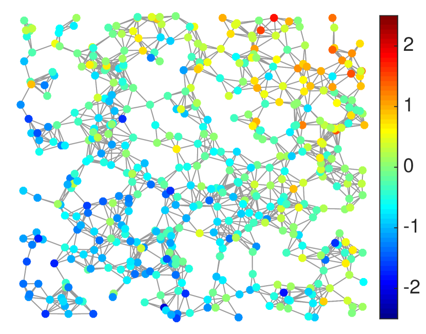
(b)

Denoised

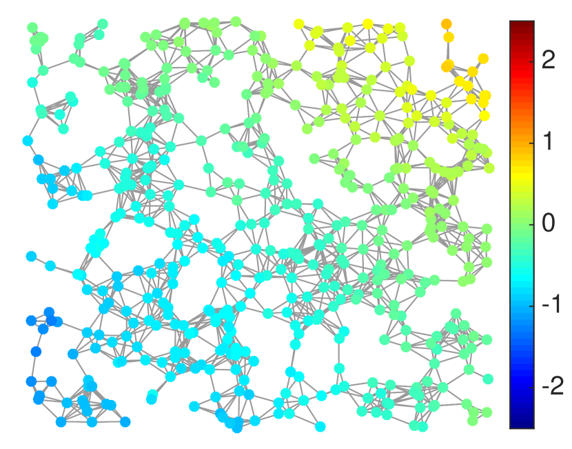
(c)

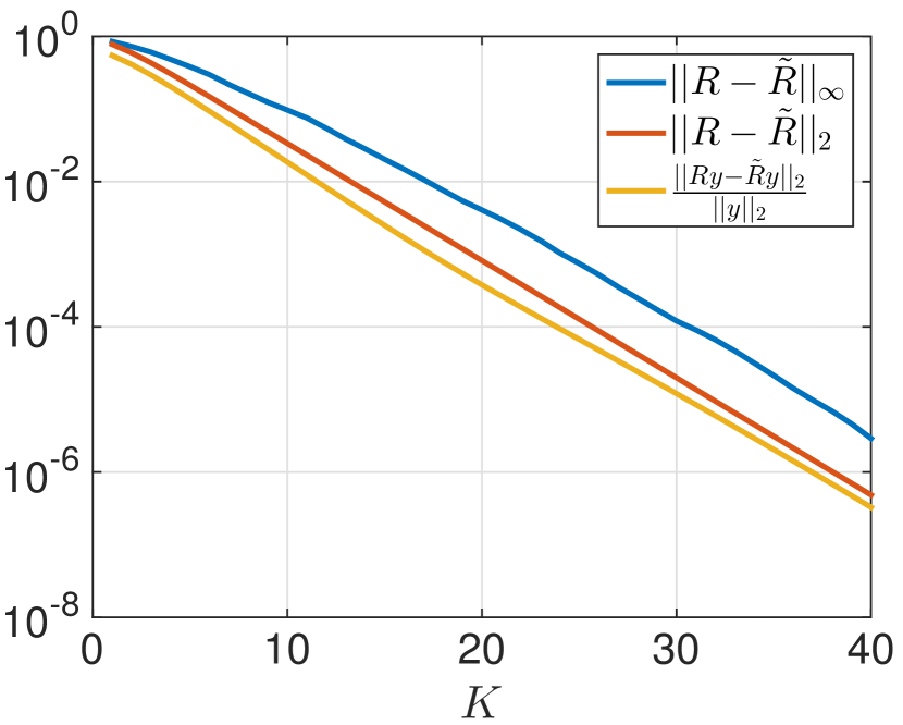
  (e)

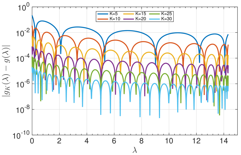
    (d)

Figure 1: Distributed denoising example. (a) The original signal with $h_{n}=n_{x}^{2}+n_{y}^{2}-1$, where $n_{x}$ and $n_{y}$ are the $x$ and $y$ coordinates of sensor node $n$. (b) The noisy signal ${\bf y}$. (c) The denoised signal $\tilde{\bf R}{\bf y}$, the Chebyshev polynomial approximation (order $K=20$) to ${\bf R}{\bf y}=\sum\limits_{\ell=0}^{N-1}\frac{1}{1+2\lambda_{\ell}}\hat{y}(\ell)\chi_{\ell}(n)$. (d) Approximation errors of shifted Chebyshev polynomial expansions of different orders for the filter $\hat{g}(\lambda_{\ell})=\frac{1}{1+2\lambda_{\ell}}$. (e) Resulting approximation errors for the graph Fourier multiplier operator and graph filtered signal.

IV-E Approximation Error

We use the following result, which bounds the spectral norm of the difference between a union of graph multiplier operators and its Chebyshev polynomial approximation, to analyze the distributed lasso problem in Section VI.

Proposition 4

Let $\mathbf{\Phi}$ be a union of $\eta$ graph multiplier operators; i.e., it has the form given in (7) for a real symmetric positive semi-definite matrix $\mathbf{P}$. Let $\tilde{\mathbf{\Phi}}$ be the order $K$ Chebyshev polynomial approximation of $\mathbf{\Phi}$. Define

$$B(K):=\max_{j=1,2,\ldots,\eta}\left\{\sup_{\lambda\in[0,\lambda_{\max}]}\left\{\left|g_{j}(\lambda)-p_{j}^{K}(\lambda)\right|\right\}\right\},$$ (38)

where $\lambda_{\max}$ is the largest eigenvalue of $\mathbf{P}$, and $p_{j}^{K}(\cdot)$ is the order $K$ Chebyshev polynomial approximation of $g_{j}(\cdot)$. Then

$$|\!|\!|{\mathbf{\Phi}}-\tilde{\mathbf{\Phi}}|\!|\!|_{2}:=\max_{\mathbf{f}\neq\mathbf{0}}\frac{\lVert({\mathbf{\Phi}}-\tilde{\mathbf{\Phi}})\mathbf{f}\rVert_{2}}{\lVert\mathbf{f}\rVert_{2}}\leq B(K)\sqrt{\eta}.$$ (39)

The proof of Proposition 4 is included in the Appendix.

Finally, note that when the multipliers $g_{j}(\cdot)$ are smooth, the Chebyshev approximations $p_{j}^{K}(\cdot)$ converge to the multipliers rapidly as $K$ increases. The following proposition characterizes this convergence.

Proposition 5 (Theorem 5.14 in [43])

If $g_{j}(\cdot)$ has $M+1$ continuous derivatives for all $j$, then $B(K)={\mathcal{O}}\left({K^{-M}}\right)$.

V Other Distributed Methods for Computing $g(\mathbf{P})\mathbf{y}$

In this section, we discuss some other methods for computing $g(\mathbf{P})\mathbf{y}$ in a distributed setting. Most of these variations are not distributed computation methods per se, but rather centralized computational methods that can be distributed in the context of the applications mentioned above.

Higham [37, Chapter 13], as well as Frommer and Simoncini [48] provide excellent introductory overviews of centralized methods to compute $g(\mathbf{P})\mathbf{y}$ for large, sparse $\mathbf{P}$. Of the methods mentioned there, we do not consider contour integral or Krylov subspace methods, which are not readily amenable to distributed computation. For example, in a distributed setting, the Lanczos method [24, 49] would require a significant amount of extra communication at each iteration to compute vector norms.

V-A Jacobi’s Iterative Method

For $\mathbf{S}=\mathbf{P}={\mathbf{\cal L}}_{\mathrm{\mathrm{norm}}}$, Zhou et al. [13] propose to solve the semi-supervised classification problem (28) through the iteration

$$\mathbf{F}^{(t+1)}=\frac{1}{1+\tau}\left[\left(\mathbf{I}_{N}-\mathbf{P}\right)\mathbf{F}^{(t)}+\tau\mathbf{Y}\right],~{}~{}~{}$$

$$~{}~{}~{}~{}~{}t=0,1,\ldots,T-1,$$ (40)

where $\mathbf{F}^{(0)}$ is arbitrary (set to $\mathbf{Y}$ in [13]). The iteration (V-A) is in fact just a particular instance of Jacobi’s iterative method (see, e.g., [50, Chapter 4]) to solve the set of linear equations

$$\left(\tau\mathbf{I}_{N}+\mathbf{P}\right)\mathbf{F}^{\mathrm{opt}}=\tau\mathbf{Y}.$$ (41)

So one alternative distributed semi-supervised classification method with $\mathbf{S}=\mathbf{P}={\mathbf{\cal L}}_{\mathrm{\mathrm{norm}}}$ is to compute the iterations (V-A) in a distributed manner, with each node starting with knowledge of its row of $\mathbf{P}$ and $\mathbf{Y}$. In fact, the communication cost of one iteration of (V-A) is the same as the communication cost of one iteration of the distributed computation of $\tilde{\mathbf{R}}\mathbf{Y}$ (lines 6 and 7 of Algorithm 1).

For graph multiplier operators whose multipliers have the property $g(\lambda_{\ell})\neq 0$ for all $\ell$, the Jacobi method generalizes as follows. Suppose we wish to compute $\mathbf{Ry}$, where $\mathbf{R}$ is a graph multiplier operator with respect to $\mathbf{P}$ and with multiplier $g(\cdot)$. This is equivalent to solving the linear system of equations $g(\mathbf{P})^{-1}\mathbf{x}=\mathbf{y}$. Assuming that the entries of the matrix $\mathbf{Q}=g(\mathbf{P})^{-1}$ are convenient to evaluate (e.g., for certain rational functions $g$), let $\mathbf{Q}=\mathbf{Q}_{D}-\mathbf{Q}_{O}$, where $\mathbf{Q}_{D}$ contains the diagonal part of $\mathbf{Q}$. Then the Jacobi iteration is

$$\mathbf{x}^{(t+1)}=\mathbf{Q}_{D}^{-1}\mathbf{Q}_{O}\mathbf{x}^{(t)}+\mathbf{Q}_{D}^{-1}\mathbf{y},~{}t=0,1,\ldots,T-1.$$ (42)

One immediate drawback of Jacobi’s method, as compared with the Chebyshev polynomial method of Section IV, is that it does not always converge. The iterations in (42) converge for any $\mathbf{x}^{(0)}$ if and only if the spectral radius of $\mathbf{Q}_{D}^{-1}\mathbf{Q}_{O}$ is less than one [50, Theorem 4.1]. One sufficient condition for the latter to be true is that $\mathbf{Q}$ is strictly diagonally dominant, as is the case for example when $\mathbf{P}={\mathbf{\cal L}}$ and $g(\lambda_{\ell})=\frac{\tau}{\tau+\lambda_{\ell}}$. Additionally, it may be too expensive computationally to evaluate the matrix $\mathbf{Q}$, or it may be a dense matrix, in which case the communication cost of a distributed method becomes prohibitive. For example, if $g=e^{-t\lambda}$, it is not efficient to fully evaluate $\mathbf{Q}$ and so this method is not applicable.

V-B Jacobi’s Iterative Method with Chebyshev Acceleration

When Jacobi’s method does converge, we can accelerate (42) using the following algorithm [51, Algorithm 6.7]. Let $\rho$ be an upper bound on the spectral radius of $\mathbf{Q}_{D}^{-1}\mathbf{Q}_{O}$, and define $\xi^{(0)}:=1$, $\xi^{(1)}:=\rho$, and $\mathbf{x}^{(1)}:=\mathbf{Q}_{D}^{-1}\mathbf{Q}_{O}\mathbf{x}^{(0)}+\mathbf{Q}_{D}^{-1}\mathbf{y}$. Then for $t\geq 1$, let

$$\xi^{(t+1)} =\frac{1}{\frac{2}{\rho\xi^{(t)}}-\frac{1}{\xi^{(t-1)}}},\hbox{ and }$$

$$\mathbf{x}^{(t+1)} =\frac{2\xi^{(t+1)}}{\rho\xi^{(t)}}\mathbf{Q}_{D}^{-1}\mathbf{Q}_{O}\mathbf{x}^{(t)}-\frac{\xi^{(t+1)}}{\xi^{(t-1)}}\mathbf{x}^{(t-1)}$$

$$\quad\quad+\frac{2\xi^{(t+1)}}{\rho\xi^{(t)}}\mathbf{Q}_{D}^{-1}\mathbf{y}.$$ (43)

To distribute (V-B), each node $n$ must first learn $Q_{nn}$ and the $n^{\mathrm{th}}$ row of $\mathbf{Q}_{O}$. For example, when $\mathbf{P}={\mathbf{\cal L}}_{\mathrm{\mathrm{norm}}}$ and $g(\lambda_{\ell})=\frac{\tau}{\tau+\lambda_{\ell}}$, as in (V-A), $Q_{nn}=\frac{\tau+1}{\tau}$ for all $n$, and the $n^{\mathrm{th}}$ row of $\mathbf{Q}_{O}$ is just $-\frac{1}{\tau}$ times the $n^{\mathrm{th}}$ row of ${\mathbf{\cal L}}_{\mathrm{\mathrm{norm}}}$. An additional challenge in a distributed setting may be to calculate the bound $\rho$.

Note that while this method and the method of Section IV share the same namesake, the use of the Chebyshev polynomials in the two is different. In Section IV, we use Chebyshev polynomials to approximate the multiplier, whereas this method improves the convergence speed of the Jacobi method by using Chebyshev polynomials to choose the weights it uses to form the iterates in (V-B) as weighted linear combinations of the iterates in (42). See Section 6.5.6 of [51] for more details.

$\mathbf{S}={\mathbf{\cal L}}_{\mathrm{norm}}$

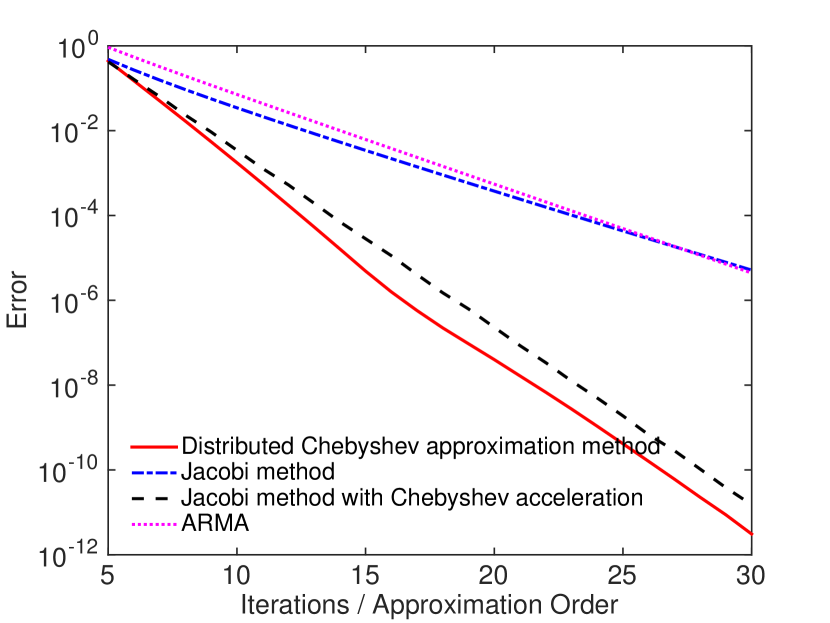
(a)

$\mathbf{S}={\mathbf{\cal L}}^{2}$

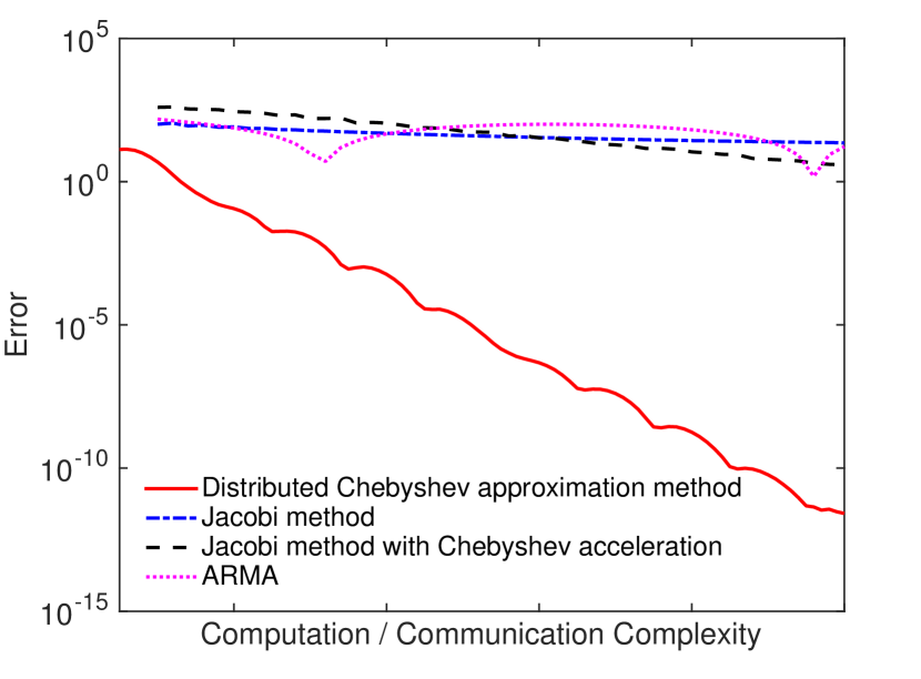
(b)

$\mathbf{S}=\left(2\mathbf{I}_{N}-{\mathbf{\cal L}}_{\mathrm{norm}}\right)^{-3}$

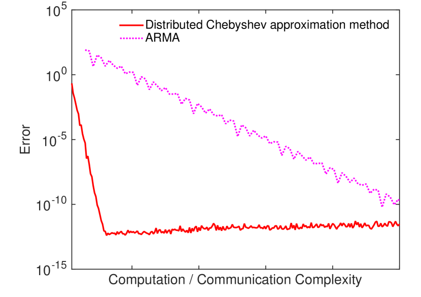
(c)

Figure 2: Four different distributed methods to approximately compute $\mathbf{Ry}$, where $\mathbf{R}$ is a graph multiplier operator with respect to $\mathbf{P}$ for different choices of $\mathbf{P}$. In all cases, the multiplier is $g(\lambda_{\ell})=\frac{\tau}{\tau+h(\lambda_{\ell})}$. In (a), the error shown is $\lVert\mathbf{f}^{(K)}-\mathbf{f}\rVert_{2}$, where $\mathbf{f}^{(K)}$ is either $\tilde{\mathbf{R}}\mathbf{y}$ with an order $K$ approximation for our distributed Chebyshev approximation method, or the result of the $K^{\mathrm{th}}$ iteration for the Jacobi and ARMA methods. In (b) and (c), since iterations of the different algorithms have different computation and communication complexities, we normalize to a common scale.

V-C Polynomial Approximation Variants

Other orthogonal polynomials can also be used to generate approximations via truncated expansions. For example, [52] uses Laguerre polynomials to approximate matrix exponentials. One advantage of this method is that Laguerre polynomials are orthonormal on $[0,\infty)$, so no upper bound on the spectrum is required. However, in the applications we consider, it is usually not hard to generate the upper bound $\overline{\lambda_{\max}}$.

In [53], Chen et al. first approximate the filter $g$ by a polynomial spline, and then compute orthogonal expansion coefficients of the spline in order to avoid the numerical integration involved in computing, e.g., the Chebyshev coefficients $\{c_{k}\}$ in (32). The conjugate residual-type algorithm of [54] also uses the spline approach. However, in [54], the order $K+1$ polynomial approximation of a highpass filter $g$ takes the form $\tilde{g}(\lambda)=\lambda\varphi(\lambda)$, where $\varphi$ is an order $K$ polynomial, forcing $\tilde{g}(0)$ to be equal to zero. If $g$ is a lowpass filter such as $g(\lambda)=e^{-\tau\lambda}$, then [54] takes the approximation to be of the form $\tilde{g}(\lambda)=1-\lambda\varphi(\lambda)$, with $\varphi$ an order $K$ polynomial, once again guaranteeing zero approximation error at $\lambda=0$. This technique can be extended to bandpass filters by splitting the spectrum up into separate intervals, eventually leading to a three term recurrence with new weights that can be computed offline. A distributed implementation then carries the same communication cost as the single Chebyshev polynomial approximation.

V-D Rational Approximations

An alternative to a polynomial approximation is a rational approximation (see, e.g., [48, Section 3.4]) of the form

$$g(\lambda)\approx\frac{{\cal N}_{\mu}(\lambda)}{{\cal D}_{\nu}(\lambda)}=:\tilde{\tilde{g}}(\lambda),$$ (44)

where ${\cal N}_{\mu}$ and ${\cal D}_{\nu}$ are polynomials of degree $\mu$ and $\nu$, respectively. In the graph signal processing literature, references such as [34, 35] refer to filters of the form (44) as infinite impulse response filters, since we can not write

$$\tilde{\tilde{g}}(\mathbf{P})=c_{0}\mathbf{I}+\sum_{k=1}^{K}c_{k}\mathbf{P}^{k},$$ (45)

for any choice of the order $K$ and series of coefficients $\{c_{k}\}$.

One benefit of rational approximations of the form (44) is that they tend to provide better approximations than polynomials of lower orders, especially when $g$ features a singularity close to the spectrum of $\mathbf{P}$. However, a major drawback is they tend to require extra subiterations, resulting in increased communication cost. For example, to compute $\mathbf{x}={\cal D}_{\nu}^{-1}(\mathbf{P})\mathbf{y}$, [34] uses gradient descent to iteratively solve

$$\operatorname*{argmin}_{\mathbf{x}}||{\cal D}_{\nu}(\mathbf{P})\mathbf{x}-\mathbf{y}||^{2}.$$ (46)

Yet, [34] estimates the number of iterations required to solve (46) as $\frac{\max_{\ell=0,1,\ldots,N-1}\{{\cal D}_{\nu}(\lambda_{\ell})^{2}\}}{\min_{\ell=0,1,\ldots,N-1}\{{\cal D}_{\nu}(\lambda_{\ell})^{2}\}}$. Each of these iterations requires twice as much communication as the full distributed computation of an order $\nu$ matrix polynomial computation via Algorithm 1 (with $\eta=1$). So even when ${\cal N}_{\mu}$ and ${\cal D}_{\nu}$ are taken to be lower order polynomials, the communication requirements may still be significantly higher than a higher order polynomial approximation (where ${\cal D}_{\nu}(\lambda)=1$).

Some filters of the form (44) with $\mu\leq K$ and $\nu=K$ can also be written as

$$\tilde{\tilde{g}}(\lambda)=\sum_{k=1}^{K}\frac{2r_{k}}{{\lambda_{\max}-\lambda_{\min}}-2\lambda-2p_{k}},$$ (47)

for some coefficient sequences $\{r_{k}\}$ and $\{p_{k}\}$. Loukas et al. [35] refer to such filters as parallel autoregressive moving average graph filters (ARMA) of order $K$, and show that if for all $k$, $|p_{k}|>\frac{\lambda_{\max}-\lambda_{\min}}{2}$, then $\mathbf{x}=\tilde{\tilde{g}}(\mathbf{P})\mathbf{y}$ can be computed by iterating the following recursion for each term in the summation on the right-hand side of (47):

$$\mathbf{x}_{k}^{(t+1)} =\frac{1}{p_{k}}\left[\left(\frac{\lambda_{\max}-\lambda_{\min}}{2}\right)\mathbf{I}-\mathbf{P}\right]\mathbf{x}_{k}^{(t)}-\frac{r_{k}}{p_{k}}\mathbf{y},$$

$$~{}~{}~{}~{}~{}~{}~{}~{}~{}~{}~{}~{}~{}~{}~{}~{}~{}~{}~{}~{}~{}~{}~{}~{}~{}~{}~{}~{}~{}~{}~{}~{}~{}t=0,1,\ldots,T-1$$ (48)

and then summing these results to find $\mathbf{x}=\sum_{k=1}^{K}\mathbf{x}_{k}$. Once again, these ARMA filters have the potential to yield a better approximation than a finite impulse response filter of the form on the right-hand side of (45) with the same order $K$; however, they require $T$ times the communication, where $T$ is the number of times one must iterate (V-D) to convergence.

V-E Numerical Comparison

We consider the same random sensor network shown in Figure 1, and we generate a signal $\mathbf{f}$ on the vertices of the graph with the components of $\mathbf{f}$ independently and identically sampled from a uniform distribution on $[-10,10]$. For different choices of $h(\cdot)$ and $\mathbf{P}={\mathbf{\cal L}}$ or $\mathbf{P}={\mathbf{\cal L}}_{\mathrm{norm}}$, we define

$$\mathbf{y}:=\left(\mathbf{I}_{500}+\frac{1}{\tau}h(\mathbf{P})\right)\mathbf{f}=g(\mathbf{P})\mathbf{f},$$

with $\tau=0.5$ and $g(\lambda)=\frac{\tau+h(\lambda)}{\tau}$. Then, starting with $\mathbf{y}$, we iteratively compute an approximation to $\mathbf{f}$ in four different distributable ways: 1) $\tilde{\mathbf{R}}\mathbf{y}$, where $\tilde{\mathbf{R}}$ is the Chebyshev approximation to $\mathbf{R}=g(\mathbf{P})^{-1}$; 2) with the Jacobi iteration (42); 3) with the Jacobi iteration with Chebyshev acceleration (V-B); and 4) the ARMA iteration (V-D).

When $P={\mathbf{\cal L}}_{\mathrm{norm}}$ and $\mathbf{S}=h(\mathbf{P})={\mathbf{\cal L}}_{\mathrm{norm}}$, the filter $g^{-1}$ is the ratio of a constant and a first order polynomial, so we can take $K=1$ in (47). Taking the initial guess $\mathbf{x}^{(0)}$ to be $\mathbf{y}$ and $\lambda_{\min}=0$, the iteration (V-D) becomes

$$\mathbf{x}^{(t+1)} =\frac{2}{\tau+\lambda_{\max}}\left[\left(\frac{\lambda_{\max}}{2}\mathbf{I}-\mathbf{P}\right)\mathbf{x}^{(t)}+\tau\mathbf{y}\right]$$

$$=\frac{2\tau}{\tau+\lambda_{\max}}\mathbf{y}+\frac{\lambda_{\max}}{\tau+\lambda_{\max}}\mathbf{x}^{(t)}-\frac{2}{\tau+\lambda_{\max}}\mathbf{P}\mathbf{x}^{(t)}.$$

In this case, the communication requirements of our method with Chebyshev approximation order $K$ are equal to the communication requirements of $T=K$ iterations of the latter three methods, so we plot the errors $\lVert\mathbf{f}^{(K)}-\mathbf{f}\rVert_{2}$ (where $\mathbf{f}^{(K)}$ corresponds to $\tilde{\mathbf{R}}\mathbf{y}$ with an order $K$ approximation in the first case or the result of the $K^{\mathrm{th}}$ iteration in the latter three cases) on the same axes in Figure 2(a).

When $P={\mathbf{\cal L}}$ and $\mathbf{S}=h(\mathbf{P})={\mathbf{\cal L}}^{2}$, computing $\mathbf{Q}_{O}\mathbf{x}^{(t)}$ in (42) and (V-B) requires computing $\mathbf{W}\mathbf{x}^{(t)}$, which requires twice the communication and computation of a single iteration of Algorithm 1 for the polynomial approximation. For the ARMA approach, we can write the filter $g(\lambda)=\frac{\tau}{\tau+\lambda^{2}}$ exactly in the form of (47) with $p_{1}=\sqrt{\tau}i+\frac{\lambda_{\max}}{2},~{}p_{2}=-\sqrt{\tau}i+\frac{\lambda_{\max}}{2},~{}r_{1}=-\frac{\sqrt{\tau}i}{2}$, and $r_{2}=\frac{\sqrt{\tau}i}{2}$.

When $P={\mathbf{\cal L}}_{\mathrm{norm}}$ and $\mathbf{S}=h(\mathbf{P})=\left(2\mathbf{I}_{500}-{\mathbf{\cal L}}_{\mathrm{norm}}\right)^{-3}$ (a three-step random walk process), the Jacobi method does not converge. We have $h(\lambda)=(2-\lambda)^{-3}$, and thus

$$g(\lambda)=\frac{\tau}{\tau+h(\lambda_{\ell})}=1-\frac{2}{(2-\lambda)^{3}+2},$$

the last term of which can be written as a third order ARMA filter.

Figure 2 compares the approximation error to the communication/computation complexity for each of these methods and choices of $\mathbf{S}$. In these experiments, not only does our proposed method always converge, but it converges faster and with less communication than the alternative methods we tested.

VI Distributed Lasso

In Section III, we presented a number of distributed signal processing tasks that could be represented as a single application of a union of graph multiplier operators. In this section, we present a distributed wavelet denoising example that requires repeated applications of unions of graph multiplier operators and their adjoints. Recall that the distributed Tikhonov regularization method from Section III-A is an efficient way to denoise a signal when we have a priori information that the underlying signal is globally smooth. The distributed wavelet denoising method is better suited to situations where we start with a prior belief that the signal is not globally smooth, but rather piecewise smooth, which corresponds to the signal being sparse in the spectral graph wavelet domain [23].

The spectral graph wavelet transform, defined in [23] is precisely of the form of $\mathbf{\Phi}$ in (21). Namely, it is composed of one multiplier, $h(\cdot)$, that acts as a lowpass filter to stably represent the signal’s low frequency content, and $J$ wavelet operators, defined by $g_{j}(\lambda_{\ell})=g(t_{j}\lambda_{\ell})$, where $\{t_{j}\}_{j=1,2,\ldots,J}$ is a set of scales and $g(\cdot)$ is the wavelet multiplier that acts as a bandpass filter.

The most common way to incorporate a sparse prior in a centralized setting is to regularize via a weighted version of the least absolute shrinkage and selection operator (lasso) [55], also called basis pursuit denoising [56]:

$$\operatorname*{argmin}_{\mathbf{a}}~{}\frac{1}{2}\lVert\mathbf{y}-\mathbf{\Phi}^{*}{\mathbf{a}}\rVert_{2}^{2}+\lVert{\mathbf{a}}\rVert_{1,\boldsymbol{\mu}}~{},$$ (49)

where $\lVert{\mathbf{a}}\rVert_{1,\boldsymbol{\mu}}:=\sum_{i=1}^{N(J+1)}\mu_{i}\left|{a}_{i}\right|$ and $\mu_{i}>0$ for all $i$. The optimization problem in (49) can be solved for example by iterative soft thresholding [57]. The initial estimate of the wavelet coefficients ${\mathbf{a}}^{(0)}$ is arbitrary, and at each iteration of the soft thresholding algorithm, the update of the estimated wavelet coefficients is given by

$${a}_{i}^{(\beta)}=\mathcal{S}_{{\mu}_{i}{\gamma}}\left(\Bigl{(}{{a}}^{(\beta-1)}+{\gamma}{\Phi}\left[{y}-{\Phi}^{*}{{a}}^{(\beta-1)}\right]\Bigr{)}_{i}\right),$$

$$i=1,2,\ldots,N(J+1);~{}\beta=1,2,\ldots$$ (50)

where ${\gamma}$ is the step size and $\mathcal{S}_{{\mu}_{i}{\gamma}}$ is the shrinkage or soft thresholding operator

$$\mathcal{S}_{{\mu}_{i}{\gamma}}(z):=\left\{\begin{array}[]{ll}0&,\mbox{ if }\mid z\mid\leq{\mu}_{i}{\gamma}\\ z-\mbox{sgn}(z){\mu}_{i}{\gamma}&,\mbox{ o.w.}\end{array}\right..$$

The iterative soft thresholding algorithm converges to ${{\mathbf{a}}}_{*}$, the minimizer of (49), if ${\gamma}<\frac{2}{{\lVert\mathbf{\Phi}^{*}\rVert^{2}}}$ [58]. The final denoised estimate of the signal is then given by $\mathbf{\Phi}^{*}{{\mathbf{a}}}_{*}$.

We now turn to the issue of how to implement the above algorithm in a distributed fashion by sending messages between neighbors in the network. One option would be to use the distributed lasso algorithm of [29, 30], which is a special case of the alternating direction method of multipliers [59, p. 253]. In every iteration of that algorithm, each node transmits its current estimate of all the wavelet coefficients to its local neighbors. With the spectral graph wavelet transform, that method requires $2\lvert{{\mathcal{E}}}\rvert$ total messages at every iteration, with each message being a vector of length $N(J+1)$. A method where the amount of communicated information does not grow with $N$ (beyond the number of edges, $\lvert{{\mathcal{E}}}\rvert$) would be highly preferable.

The Chebyshev polynomial approximation of the spectral graph wavelet transform allows us to accomplish this goal. Our approach, which is summarized in Algorithm 3, is to approximate $\mathbf{\Phi}$ by $\tilde{\mathbf{\Phi}}$, and use the distributed implementation of the approximate wavelet transform and its adjoint to perform iterative soft thresholding in order to solve

$$\operatorname*{argmin}_{\tilde{\mathbf{a}}}~{}\frac{1}{2}\lVert\mathbf{y}-\tilde{\mathbf{\Phi}}^{*}\tilde{\mathbf{a}}\rVert_{2}^{2}+\lVert\tilde{\mathbf{a}}\rVert_{1,\boldsymbol{\mu}}.$$ (52)

In the first soft thresholding iteration, each node $n$ must learn $(\tilde{{\Phi}}{y})_{(j-1)N+n}$ at all scales $j$, via Algorithm 1. These coefficients are then stored for future iterations. In the $\beta^{\mathrm{th}}$ iteration, each node $n$ must learn the $J+1$ coefficients of $\tilde{\mathbf{\Phi}}\tilde{\mathbf{\Phi}}^{*}\tilde{\mathbf{a}}^{(\beta-1)}$ centered at $n$, by sequentially applying the operators $\tilde{\mathbf{\Phi}}^{*}$ and $\tilde{\mathbf{\Phi}}$ in a distributed manner via Algorithms 2 and 1, respectively. When a stopping criterion for the soft thresholding is satisfied, the adjoint operator $\tilde{\mathbf{\Phi}}^{*}$ is applied again in a distributed manner to the resulting coefficients $\tilde{{{\mathbf{a}}}}_{*}$, and node $n$’s denoised estimate of its signal is $\left(\tilde{{\Phi}}^{*}\tilde{{{{a}}}}_{*}\right)_{n}$. The stopping criterion may simply be a fixed number of iterations, or it may be when $\left|\left(\tilde{{\Phi}}^{*}\tilde{a}^{(\beta)}\right)_{n}-\left(\tilde{{\Phi}}^{*}\tilde{a}^{(\beta-1)}\right)_{n}\right|<\epsilon$ for all $n$ and some small $\epsilon$. Finally, note that we could also optimize the weights $\boldsymbol{\mu}$ by performing distributed cross-validation, as discussed in [29, 30].

We now examine the communication requirements of this approach. Recall from Section IV-B that $2K\lvert{{\mathcal{E}}}\rvert$ messages of length 1 are required to compute $\tilde{\mathbf{\Phi}}\mathbf{y}$ in a distributed fashion. Distributed computation of $\tilde{\mathbf{\Phi}}\tilde{\mathbf{\Phi}}^{*}\tilde{\mathbf{a}}^{(\beta-1)}$, the other term needed in the iterative thresholding update (VI), requires $2K\lvert{{\mathcal{E}}}\rvert$ messages of length $J+1$ and $2K\lvert{{\mathcal{E}}}\rvert$ messages of length $1$. The final application of the adjoint operator $\tilde{\mathbf{\Phi}}^{*}$ to recover the denoised signal estimates requires another $2K\lvert{{\mathcal{E}}}\rvert$ messages, each a vector of length $J+1$. Therefore, the Chebyshev polynomial approximation to the spectral graph wavelet transform enables us to iteratively solve the weighted lasso in a distributed manner where the communication workload only scales with the size of the network through $\lvert{\mathcal{E}}\rvert$, and is otherwise independent of the network dimension $N$.

The reconstructed signal in Algorithm 3 is $\tilde{\mathbf{\Phi}}^{*}\tilde{\mathbf{a}}_{*}$, where $\tilde{\mathbf{a}}_{*}$ is the solution to the lasso problem (52). A natural question is how good of an approximation $\tilde{\mathbf{\Phi}}^{*}\tilde{\mathbf{a}}_{*}$ is to ${\mathbf{\Phi}}^{*}{\mathbf{a}}_{*}$, where ${\mathbf{a}}_{*}$ is the solution to the original lasso problem (49). The following proposition bounds the squared distance between these two quantities by a term proportional to the spectral norm of the difference between the exact and approximate spectral graph wavelet operators.

Proposition 6

$\lVert\tilde{\mathbf{\Phi}}^{*}\tilde{\mathbf{a}}_{*}-{\mathbf{\Phi}}^{*}{\mathbf{a}}_{*}\rVert_{2}^{2}\leq C|\!|\!|\tilde{\mathbf{\Phi}}-\mathbf{\Phi}|\!|\!|_{2}$, where $|\!|\!|\cdot|\!|\!|_{2}$ is the spectral norm, and the constant $C=\frac{\lVert\mathbf{y}\rVert_{2}^{3}}{\min_{i}\mu_{i}}$.

Combining Proposition 6, whose proof is included in the Appendix, with (39), we have

$$\lVert\tilde{\mathbf{\Phi}}^{*}\tilde{\mathbf{a}}_{*}-{\mathbf{\Phi}}^{*}{\mathbf{a}}_{*}\rVert_{2}^{2}\leq\frac{\lVert\mathbf{y}\rVert_{2}^{3}}{\min_{i}\mu_{i}}B(K)\sqrt{J+1}.$$ (53)

Thus, as we increase the approximation order $K$, $B(K)$ and the right-hand side of (53) tend toward zero (at a speed dependent on the smoothness of the graph wavelet multipliers $g(\cdot)$ and $h(\cdot)$).

Finally, to illustrate the distributed lasso, we consider a numerical example. We use the same 500 node sensor network as in Section IV-D. This time, however, the underlying signal is piecewise smooth, but not globally smooth, with the $n^{\mathrm{th}}$ component given by

$$f_{n}^{0}=\begin{cases}-2n_{x}+0.5,&\hbox{ if }n_{y}\geq 1-n_{x}\\ n_{x}^{2}+n_{y}^{2}+0.5,&\hbox{ if }n_{y}<1-n_{x}\end{cases}.$$

We corrupt each component of the signal $\mathbf{f}^{0}$ with uncorrelated additive Gaussian noise with mean zero and standard deviation 0.5. We then solve problem (52) in a distributed manner using Algorithm 3. We use a spectral graph wavelet transform with 6 wavelet scales, implemented by the Graph Signal Processing Toolbox [60]. In Algorithm 3, we run 300 soft thresholding iterations and take $\gamma=0.2$, $\mu_{i}=0.75$ for all the wavelet coefficients, and $\mu_{i}=0.01$ for all the scaling coefficients. We do not perform any distributed cross-validation to optimize the weights $\boldsymbol{\mu}$. We repeated this entire experiment 1000 times, with a new random graph and random noise each time. The average mean square errors were 0.250 for the noisy signals, 0.098 for the estimates produced by the Tikhonov regularization method (24), 0.088 for the denoised estimates produced by the distributed lasso with the exact wavelet operator, and 0.079 for the denoised estimates produced by the distributed lasso with the approximate wavelet operator with $K=15$. Note that the approximate solution does not necessarily result in a higher mean square error than the exact solution.

Algorithm 3 Distributed lasso

Inputs at node $n$: $y_{n}$, ${\mathbf{\cal L}}_{n,m}~{}\forall m$, $\left\{\mu_{(j-1)N+n}\right\}_{j=1,2,\ldots,J+1}$,
$\overline{\lambda_{\max}}$, $\gamma$, and $\left\{c_{k,j}\right\}_{j=1,2,\ldots,J+1;~{}k=0,1,\ldots,K}$
Outputs at node $n$: $y_{n*}$, the denoised estimate of $f^{0}_{n}$

1:  Arbitrarily initialize $\left\{\left(\tilde{{a}}^{(0)}\right)_{(j-1)N+n}\right\}_{j=1,2,\ldots,J+1}$

2:  Set $\beta=1$

3:  Compute and store $\left\{\left({{\Phi}}{y}\right)_{(j-1)N+n}\right\}_{j=1,2,\ldots,J+1}$ via Algorithm 1

4:  while stopping criterion not satisfied do

5:     Compute and store

$$\left\{\left(\tilde{{\Phi}}\tilde{{\Phi}}^{*}\tilde{{a}}^{(\beta-1)}\right)_{(j-1)N+n}\right\}_{j=1,2,\ldots,J+1}$$

via Algorithm 2, followed by Algorithm 1

6:     for $j=1,2,\ldots,J+1$ do

7:        Compute and store

$$\left(\tilde{{a}}^{(\beta)}\right)_{(j-1)N+n}$$

$$=\mathcal{S}_{\left({\mu}_{(j-1)N+n}\right){\gamma}}\left(\begin{array}[]{l}{\tilde{a}}^{(\beta-1)}_{(j-1)N+n}\\ +{\gamma}\left(\tilde{{\Phi}}{y}\right)_{(j-1)N+n}\\ -{\gamma}\left(\tilde{{\Phi}}\tilde{{\Phi}}^{*}\tilde{{a}}^{(\beta-1)}\right)_{(j-1)N+n}\end{array}\right)$$

8:     end for

9:     Set $\beta=\beta+1$

10:  end while

11:  for $j=1,2,\ldots,J+1$ do

12:     Set $\left(\tilde{{a}}_{*}\right)_{(j-1)N+n}=\left(\tilde{{a}}^{(\beta)}\right)_{(j-1)N+n}$

13:  end for

14:  Compute and store $y_{n*}=\left(\tilde{{\Phi}}^{*}\tilde{{a}}_{*}\right)_{n}$ via Algorithm 2

15:  Output $y_{n*}$

VII Concluding Remarks

We presented a novel method to distribute a class of linear operators called unions of graph multiplier operators. The main idea is to approximate the graph multipliers by Chebyshev polynomials, whose recurrence relations make them readily amenable to distributed computation. Key takeaways from the discussion and application examples include:

• A number of distributed signal processing tasks can be represented as distributed applications of unions of graph multiplier operators (and their adjoints) to signals on weighted graphs. Examples include distributed smoothing, denoising, inverse filtering, and semi-supervised learning.

• Graph Fourier multiplier operators are the graph analog of filter banks, as they reshape functions’ frequencies through multiplication in the Fourier domain.

• The amount of communication required to perform the distributed computations only scales with the size of the network through the number of edges of the communication graph, which is usually sparse. Therefore, the method is well suited to large-scale networks.

• The approximate graph multiplier operators closely approximate the exact operators in practice, and for graph multiplier operators with smooth multipliers, an upper bound on the spectral norm of the difference of the approximate and exact operators decreases rapidly as we increase the Chebyshev approximation order.

VIII Appendix

Proof:

The objective function in (24) is convex in $\mathbf{f}$. Differentiating with respect to $\mathbf{f}$ shows that $\mathbf{f}_{*}$ is a solution to

$${\mathbf{\cal L}}^{r}\mathbf{f}_{*}+\frac{\tau}{2}(\mathbf{f}_{*}-\mathbf{y})=0$$ (54)

if and only if it is a solution to (24). Rearranging (54) gives $({\mathbf{\cal L}}^{r}+\frac{\tau}{2}I)\mathbf{f}_{*}=\frac{\tau}{2}\mathbf{y}$ and hence $\mathbf{f}_{*}=\frac{\tau}{2}({\mathbf{\cal L}}^{r}+\frac{\tau}{2}I)^{-1}\mathbf{y}$. This concludes the proof by noting that $\frac{\tau}{2}({\mathbf{\cal L}}^{r}+\frac{\tau}{2}I)^{-1}=g({\mathbf{\cal L}})$, with $g(\lambda)=\frac{\tau}{2}\frac{1}{\frac{\tau}{2}+\lambda^{r}}=\frac{\tau}{\tau+2\lambda^{r}}.$ ∎

Proof:

As in Proposition 2, the objective function in (26) is convex in $\mathbf{f}$. Differentiating it with respect to $\mathbf{f}$, we have that (26) is equivalent to

$${\mathbf{\cal L}}^{r}\mathbf{f}_{*}+\frac{\tau}{2}\mathbf{\Psi}^{*}(\mathbf{\Psi f}_{*}-\mathbf{y})=0.$$ (55)

Because ${\mathbf{\cal L}}$ is symmetric, $\mathbf{\Psi}=g_{{\Psi}}({\mathbf{\cal L}})$ is symmetric as well, allowing us to rearrange (55) as $\big{(}{\mathbf{\cal L}}^{r}+\frac{\tau}{2}g_{{\Psi}}({\mathbf{\cal L}})^{2}\big{)}\mathbf{f}_{*}=\frac{\tau}{2}g_{{\Psi}}({\mathbf{\cal L}})\mathbf{y}.$ In turn, $\mathbf{f}_{*}=\frac{\tau}{2}\big{(}{\mathbf{\cal L}}^{r}+\frac{\tau}{2}g_{{\Psi}}({\mathbf{\cal L}})^{2}\big{)}^{-1}g_{{\Psi}}({\mathbf{\cal L}})\mathbf{y}=h({\mathbf{\cal L}})\mathbf{y}$ with $h(\lambda)=\frac{\tau g_{{\Psi}}(\lambda)}{\tau g_{{\Psi}}^{2}(\lambda)+2\lambda^{r}}$. ∎

Proof:

From the definition of matrix functions, it follows for any $g$ defined on the eigenvalues $\lambda_{0},\ldots,\lambda_{N-1}$ of $\mathbf{P}$ that

$$|\!|\!|g(\mathbf{P})|\!|\!|_{2} =|\!|\!|\text{diag}\big{(}g(\lambda_{0}),\ldots,g(\lambda_{N-1})\big{)}|\!|\!|_{2}$$

$$=\max_{\ell\in\{0,1,\ldots,N-1\}}|g(\lambda_{\ell})|\leq\sup_{\lambda\in[0,\lambda_{\max}]}|g(\lambda)|.$$ (56)

Recall that $\mathbf{\Phi}:=\left[\mathbf{\Psi}_{1};\mathbf{\Psi}_{2};\ldots;\mathbf{\Psi}_{\eta}\right]$ and $\tilde{\mathbf{\Phi}}:=\left[\tilde{\mathbf{\Psi}}_{1};\tilde{\mathbf{\Psi}}_{2};\ldots;\tilde{\mathbf{\Psi}}_{\eta}\right]$ are $\eta N\times N$ matrices composed of the $N\times N$ submatrices $\mathbf{\Psi}_{j}:=g_{j}(\mathbf{P})$ and $\tilde{\mathbf{\Psi}}_{j}:=p_{j}^{K}(\mathbf{P})$, respectively. Using (56) and the definition (38) of $B(K)$, we obtain

$$|\!|\!|\mathbf{\Psi}_{j}-\tilde{\mathbf{\Psi}}_{j}|\!|\!|_{2}=|\!|\!|(g_{j}-p_{j}^{K})(\mathbf{P})|\!|\!|_{2}\leq B(K)$$

for every $j\in\{1,2,\ldots,\eta\}$. In turn, using norm inequalities for block matrices [61, Fact 9.10.2], it follows that

$$|\!|\!|{\mathbf{\Phi}}-\tilde{\mathbf{\Phi}}|\!|\!|_{2}^{2}\leq\sum_{j=1}^{\eta}|\!|\!|{\mathbf{\Psi}_{j}}-\tilde{\mathbf{\Psi}_{j}}|\!|\!|_{2}^{2}\leq\eta B(K),$$

which completes the proof. ∎

Proof:

The solutions $\mathbf{a}_{*}$ to (49) and $\tilde{\mathbf{a}}_{*}$ to (52) are not unique; however, their images $\mathbf{\Phi}^{*}\mathbf{a}_{*}$ and $\tilde{\mathbf{\Phi}}^{*}\tilde{\mathbf{a}}_{*}$ are unique. To see this, for example for $\mathbf{\Phi}^{*}\mathbf{a}_{*}$, we can write (49) equivalently as

$$\operatorname*{argmin}_{\mathbf{a},\mathbf{b}} ~{}\frac{1}{2}\lVert\mathbf{y}-\mathbf{b}\rVert_{2}^{2}+\lVert{\mathbf{a}}\rVert_{1,\boldsymbol{\mu}}$$

   s.t. $$~{}\mathbf{b}=\mathbf{\Phi}^{*}{\mathbf{a}}.$$

Then by the strict convexity of $\lVert\cdot\rVert_{2}^{2}$, the convexity of $\lVert\cdot\rVert_{1,\boldsymbol{\mu}}$, and Lemma 1 below, $\mathbf{\Phi}^{*}\mathbf{a}_{*}$ is unique.

Lemma 1

Let $f_{1}:\mathbb{R}^{n}\rightarrow\mathbb{R}$ be strictly convex, $f_{2}:\mathbb{R}^{m}\rightarrow\mathbb{R}$ be convex, and $\mathbf{A}\in\mathbb{R}^{n\times m}$. Then the solution $(\mathbf{x}^{*},\mathbf{y}^{*})$ to

$$\operatorname*{argmin}_{\mathbf{x}\in\mathbb{R}^{n},~{}\mathbf{y}\in\mathbb{R}^{m}} ~{}f_{1}(\mathbf{x})+f_{2}(\mathbf{y})$$ (57)

s.t. $$~{}\mathbf{x}=\mathbf{Ay}$$

is unique with respect to $\mathbf{x}^{*}$ (but not necessarily $\mathbf{y}^{*}$).

Proof:

Let $(\mathbf{x}_{1},\mathbf{y}_{1})$ and $(\mathbf{x}_{2},\mathbf{y}_{2})$ be in the set (57), and assume $\mathbf{x}_{1}\neq\mathbf{x}_{2}$. Then by linearity, $(\mathbf{x}_{3},\mathbf{y}_{3}):=\frac{1}{2}(\mathbf{x}_{1},\mathbf{y}_{1})+\frac{1}{2}(\mathbf{x}_{2},\mathbf{y}_{2})$ satisfies $\mathbf{x}_{3}=\mathbf{Ay}_{3}$, and by the strict convexity of $f_{1}(\cdot)$ and convexity of $f_{2}(\cdot)$,

$$f_{1}(\mathbf{x}_{3})+f_{2}(\mathbf{y}_{3}) <\frac{1}{2}f_{1}(\mathbf{x}_{1})+\frac{1}{2}f_{1}(\mathbf{x}_{2})+\frac{1}{2}f_{2}(\mathbf{y}_{1})+\frac{1}{2}f_{2}(\mathbf{y}_{2})$$

$$=~{}\min_{\left\{\mathbf{x}\in\mathbb{R}^{n},~{}\mathbf{y}\in\mathbb{R}^{m}:~{}\mathbf{x}=\mathbf{Ay}\right\}}f_{1}(\mathbf{x})+f_{2}(\mathbf{y}),$$

which is a contradiction. Thus, $\mathbf{x}_{1}=\mathbf{x}_{2}$. ∎

It follows from the first-order necessary and sufficient optimality equations of the lasso problem (see, e.g., [58, Proposition 5.3(iv)]) that for all $\mathbf{a}\in\mathbb{R}^{N(J+1)}$, we have

$$\langle\mathbf{y}-\mathbf{\Phi}^{*}\mathbf{a}_{*},\mathbf{\Phi}^{*}\mathbf{a}-\mathbf{\Phi}^{*}\mathbf{a}_{*}\rangle+\lVert\mathbf{a}_{*}\rVert_{1,\boldsymbol{\mu}}\leq\lVert\mathbf{a}\rVert_{1,\boldsymbol{\mu}},$$ (58)

and similarly

$$\langle\mathbf{y}-\tilde{\mathbf{\Phi}}^{*}\tilde{\mathbf{a}}_{*},\tilde{\mathbf{\Phi}}^{*}\mathbf{a}-\tilde{\mathbf{\Phi}}^{*}\tilde{\mathbf{a}}_{*}\rangle+\lVert\tilde{\mathbf{a}}_{*}\rVert_{1,\boldsymbol{\mu}}\leq\lVert\mathbf{a}\rVert_{1,\boldsymbol{\mu}}.$$ (59)

Taking $\mathbf{a}=\tilde{\mathbf{a}}_{*}$ in (58) and $\mathbf{a}={\mathbf{a}}_{*}$ in (59), summing (58) and (59), and rearranging, we have

$$\langle\mathbf{y}-\mathbf{\Phi}^{*}\mathbf{a}_{*},\mathbf{\Phi}^{*}\tilde{\mathbf{a}}_{*}-\mathbf{\Phi}^{*}\mathbf{a}_{*}\rangle+\langle\mathbf{y}-\tilde{\mathbf{\Phi}}^{*}\tilde{\mathbf{a}}_{*},\tilde{\mathbf{\Phi}}^{*}\mathbf{a}_{*}-\tilde{\mathbf{\Phi}}^{*}\tilde{\mathbf{a}}_{*}\rangle$$

$$=\lVert\mathbf{y}-{\mathbf{\Phi}}^{*}{\mathbf{a}}_{*}\rVert_{2}^{2}+\langle\mathbf{y}-\mathbf{\Phi}^{*}\mathbf{a}_{*},\mathbf{\Phi}^{*}\tilde{\mathbf{a}}_{*}-\mathbf{y}\rangle$$

$$\quad+\lVert\mathbf{y}-\tilde{\mathbf{\Phi}}^{*}\tilde{\mathbf{a}}_{*}\rVert_{2}^{2}+\langle\mathbf{y}-\tilde{\mathbf{\Phi}}^{*}\tilde{\mathbf{a}}_{*},\tilde{\mathbf{\Phi}}^{*}\mathbf{a}_{*}-\mathbf{y}\rangle\leq 0.$$ (60)

Then

$$\lVert\tilde{\mathbf{\Phi}}^{*}\tilde{\mathbf{a}}_{*}-{\mathbf{\Phi}}^{*}{\mathbf{a}}_{*}\rVert_{2}^{2}$$

$$~{}=\lVert\mathbf{y}-{\mathbf{\Phi}}^{*}{\mathbf{a}}_{*}\rVert_{2}^{2}+\lVert\mathbf{y}-\tilde{\mathbf{\Phi}}^{*}\tilde{\mathbf{a}}_{*}\rVert_{2}^{2}-2\langle\mathbf{y}-{\mathbf{\Phi}}^{*}{\mathbf{a}}_{*},\mathbf{y}-\tilde{\mathbf{\Phi}}^{*}\tilde{\mathbf{a}}_{*}\rangle$$

$$~{}\stackrel{{\scriptstyle\eqref{Eq:opt_cond_res}}}{{\leq}}\langle\mathbf{y}-{\mathbf{\Phi}}^{*}{\mathbf{a}}_{*},(\tilde{\mathbf{\Phi}}^{*}-{\mathbf{\Phi}}^{*})\tilde{\mathbf{a}}_{*}\rangle+\langle\mathbf{y}-\tilde{\mathbf{\Phi}}^{*}\tilde{\mathbf{a}}_{*},({\mathbf{\Phi}}^{*}-\tilde{\mathbf{\Phi}}^{*}){\mathbf{a}}_{*}\rangle$$

$$~{}\leq\lVert\mathbf{y}-{\mathbf{\Phi}}^{*}{\mathbf{a}}_{*}\rVert_{2}~{}|\!|\!|\tilde{\mathbf{\Phi}}^{*}-{\mathbf{\Phi}}^{*}|\!|\!|_{2}~{}\lVert\tilde{\mathbf{a}}_{*}\rVert_{2}$$

$$~{}\quad+\lVert\mathbf{y}-\tilde{\mathbf{\Phi}}^{*}\tilde{\mathbf{a}}_{*}\rVert_{2}~{}|\!|\!|{\mathbf{\Phi}}^{*}-\tilde{\mathbf{\Phi}}^{*}|\!|\!|_{2}~{}\lVert\mathbf{a}_{*}\rVert_{2}$$ (61)

$$~{}\leq\lVert\mathbf{y}\rVert_{2}~{}|\!|\!|\tilde{\mathbf{\Phi}}-\mathbf{\Phi}|\!|\!|_{2}\left(\lVert\tilde{\mathbf{a}}_{*}\rVert_{2}+\lVert\mathbf{a}_{*}\rVert_{2}\right),$$ (62)

where (61) follows from the Cauchy-Schwarz inequality, and (62) follows from the facts that $|\!|\!|A^{*}|\!|\!|_{2}=|\!|\!|A|\!|\!|_{2}$ [38, p. 309], and $\lVert\mathbf{y}-{\mathbf{\Phi}}^{*}{\mathbf{a}}_{*}\rVert_{2}\leq\lVert\mathbf{y}\rVert_{2}$ and $\lVert\mathbf{y}-\tilde{\mathbf{\Phi}}^{*}\tilde{\mathbf{a}}_{*}\rVert_{2}\leq\lVert\mathbf{y}\rVert_{2}$ by the optimality of $\mathbf{a}_{*}$ and $\tilde{\mathbf{a}}_{*}$, and the feasibility of $\mathbf{a}=\mathbf{0}$. Finally, by the uniqueness of $\mathbf{\Phi}^{*}\mathbf{a}_{*}$, $\lVert\mathbf{a}_{*}\rVert_{1,\boldsymbol{\mu}}$ is the same for all solutions $\mathbf{a}_{*}$, and

$$\big{\{}\min_{i}\mu_{i}\big{\}}\lVert\mathbf{a}_{*}\rVert_{2}$$

$$\quad\leq\lVert\mathbf{a}_{*}\rVert_{1,\boldsymbol{\mu}}\leq\frac{1}{2}\lVert\mathbf{y}-\mathbf{\Phi}^{*}\mathbf{a}_{*}\rVert_{2}^{2}+\lVert\mathbf{a}_{*}\rVert_{1,\boldsymbol{\mu}}\leq\frac{1}{2}\lVert\mathbf{y}\rVert_{2}^{2},$$ (63)

where the last inequality again follows from feasibility of $\mathbf{a}=\mathbf{0}$. The bound in (VIII) also holds for $\big{\{}\min_{i}\mu_{i}\big{\}}\lVert\tilde{\mathbf{a}}_{*}\rVert_{2}$, and substituting these into (62) yields the desired result. ∎

References

- [1] M. Rabbat and R. Nowak, “Distributed optimization in sensor networks,” in Proc. Int. Symp. Inf. Process. Sensor Netw., Berkeley, CA, Apr. 2004, pp. 20–27.
- [2] J. B. Predd, S. R. Kulkarni, and H. V. Poor, “Distributed learning in wireless sensor networks,” IEEE Signal Process. Mag., vol. 23, pp. 56–69, Jul. 2006.
- [3] R. Olfati-Saber, J. Fax, and R. Murray, “Consensus and cooperation in networked multi-agent systems,” Proc. IEEE, vol. 95, no. 1, pp. 215–233, Jan. 2007.
- [4] A. G. Dimakis, S. Kar, J. M. F. Moura, M. G. Rabbat, and A. Scaglione, “Gossip algorithms for distributed signal processing,” Proc. IEEE, vol. 98, no. 11, pp. 1847–1864, Nov. 2010.
- [5] A. Sandryhaila, S. Kar, and J. M. F. Moura, “Finite-time distributed consensus through graph filters,” in Proc. IEEE Int. Conf. Acc., Speech, and Signal Process., Florence, Italy, May 2014, pp. 1080–1084.
- [6] D. I Shuman, S. K. Narang, P. Frossard, A. Ortega, and P. Vandergheynst, “The emerging field of signal processing on graphs: Extending high-dimensional data analysis to networks and other irregular domains,” IEEE Signal Process. Mag., vol. 30, no. 3, pp. 83–98, May 2013.
- [7] A. J. Smola and R. Kondor, “Kernels and regularization on graphs,” in Proc. Ann. Conf. Comp. Learn. Theory, ser. Lect. Notes Comp. Sci., B. Schölkopf and M. Warmuth, Eds. Springer, 2003, pp. 144–158.
- [8] D. Zhou and B. Schölkopf, “A regularization framework for learning from graph data.” in Proc. ICML Workshop Stat. Relat. Learn. and Its Connections to Other Fields, Jul. 2004, pp. 132–137.
- [9] ——, “Regularization on discrete spaces,” in Pattern Recogn., ser. Lect. Notes Comp. Sci., W. G. Kropatsch, R. Sablatnig, and A. Hanbury, Eds. Springer, 2005, vol. 3663, pp. 361–368.
- [10] X. Zhu and Z. Ghahramani, “Learning from labeled and unlabeled data with label propagation,” Carnegie Mellon University, Technical Report CMU-CALD-02-107, 2002.
- [11] ——, “Semi-supervised learning using Gaussian fields and harmonic functions,” in Proc. Int. Conf. Mach. Learn., Washington, D.C., Aug. 2003, pp. 912–919.
- [12] M. Belkin, I. Matveeva, and P. Niyogi, “Regularization and semi-supervised learning on large graphs,” in Learn. Theory, ser. Lect. Notes Comp. Sci. Springer-Verlag, 2004, pp. 624–638.
- [13] D. Zhou, O. Bousquet, T. N. Lal, J. Weston, and B. Schölkopf, “Learning with local and global consistency,” in Adv. Neural Inf. Process. Syst., S. Thrun, L. Saul, and B. Schölkopf, Eds., vol. 16. MIT Press, 2004, pp. 321–328.
- [14] O. Delalleau, Y. Bengio, and N. Le Roux, “Efficient non-parametric function induction in semi-supervised learning,” in Proc. Int. Wkshp. on Artif. Intell. Stat., Barbados, Jan. 2005, pp. 96–103.
- [15] O. Chapelle, B. Schölkopf, and A. Zien, Eds., Semi-Supervised Learning. MIT Press, 2006.
- [16] R. K. Ando and T. Zhang, “Learning on graph with Laplacian regularization,” in Adv. Neural Inf. Process. Syst., B. Schölkopf, J. Platt, and T. Hofmann, Eds., vol. 19. MIT Press, 2007, pp. 25–32.
- [17] R. Johnson and T. Zhang, “On the effectiveness of Laplacian normalization for graph semi-supervised learning,” J. Mach. Learn. Res., vol. 8, pp. 1489–1517, 2007.
- [18] S. Bougleux, A. Elmoataz, and M. Melkemi, “Discrete regularization on weighted graphs for image and mesh filtering,” in Scale Space Var. Methods Comp. Vision, ser. Lect. Notes Comp. Sci., F. Sgallari, A. Murli, and N. Paragios, Eds. Springer, 2007, vol. 4485, pp. 128–139.
- [19] A. Elmoataz, O. Lezoray, and S. Bougleux, “Nonlocal discrete regularization on weighted graphs: a framework for image and manifold processing,” IEEE Trans. Image Process., vol. 17, pp. 1047–1060, Jul. 2008.
- [20] F. Zhang and E. R. Hancock, “Graph spectral image smoothing using the heat kernel,” Pattern Recogn., vol. 41, pp. 3328–3342, Nov. 2008.
- [21] G. Peyré, S. Bougleux, and L. Cohen, “Non-local regularization of inverse problems,” in Proc. ECCV’08, ser. Lect. Notes Comp. Sci., D. A. Forsyth, P. H. S. Torr, and A. Zisserman, Eds. Springer, 2008, pp. 57–68.
- [22] L. Rosasco, E. De Vito, and A. Verri, “Spectral methods for regularization in learning theory,” DISI, Università degli Studi di Genova, Italy, Technical Report DISI-TR-05-18, 2005.
- [23] D. K. Hammond, P. Vandergheynst, and R. Gribonval, “Wavelets on graphs via spectral graph theory,” Appl. Comput. Harmon. Anal., vol. 30, no. 2, pp. 129–150, Mar. 2011.
- [24] V. L. Druskin and L. A. Knizhnerman, “Two polynomial methods of calculating functions of symmetric matrices,” U.S.S.R. Comput. Maths. Math. Phys., vol. 29, no. 6, pp. 112–121, 1989.
- [25] R. Wagner, V. Delouille, and R. Baraniuk, “Distributed wavelet de-noising for sensor networks,” in Proc. IEEE Int. Conf. Dec. and Contr., San Diego, CA, Dec. 2006, pp. 373–379.
- [26] S. Barbarossa, G. Scutari, and T. Battisti, “Distributed signal subspace projection algorithms with maximum convergence rate for sensor networks with topological constraints,” in Proc. IEEE Int. Conf. Acc., Speech, and Signal Process., Taipei, Apr. 2009, pp. 2893–2896.
- [27] C. Guestrin, P. Bodik, R. Thibaux, M. Paskin, and S. Madden, “Distributed regression: an efficient framework for modeling sensor network data,” in Proc. Int. Symp. Inf. Process. Sensor Netw., Berkeley, CA, Apr. 2004, pp. 1–10.
- [28] J. B. Predd, S. R. Kulkarni, and H. V. Poor, “A collaborative training algorithm for distributed learning,” IEEE Trans. Inf. Theory, vol. 55, no. 4, pp. 1856–1871, Apr. 2009.
- [29] J. A. Bazerque, G. Mateos, and G. B. Giannakis, “Distributed lasso for in-network linear regression,” in Proc. IEEE Int. Conf. Acc., Speech, and Signal Process., Dallas, TX, Mar. 2010, pp. 2978–2981.
- [30] G. Mateos, J.-A. Bazerque, and G. B. Giannakis, “Distributed sparse linear regression,” IEEE Trans. Signal Process., vol. 58, no. 10, pp. 5262–5276, Oct. 2010.
- [31] D. Thanou and P. Frossard, “Distributed signal processing with graph spectral dictionaries,” in Proc. Allerton Conf. Comm., Contr., and Comp., Sep. 2015, pp. 1391–1398.
- [32] S. Segarra, A. G. Marques, and A. Ribeiro, “Distributed implementation of linear network operators using graph filters,” in Proc. Allerton Conf. Comm., Contr., and Comp., Sep. 2015, pp. 1406–1413.
- [33] ——, “Optimal graph-filter design and applications to distributed linear network operators,” IEEE Trans. Signal Process., May 2017.
- [34] X. Shi, H. Feng, M. Zhai, T. Yang, and B. Hu, “Infinite impulse response graph filters in wireless sensor networks,” IEEE Signal Process. Lett., vol. 22, no. 8, pp. 1113–1117, 2015.
- [35] A. Loukas, A. Simonetto, and G. Leus, “Distributed autoregressive moving average graph filters,” IEEE Signal Process. Lett., vol. 22, no. 11, pp. 1931–1935, 2015.
- [36] D. I Shuman, P. Vandergheynst, and P. Frossard, “Chebyshev polynomial approximation for distributed signal processing,” in Proc. Int. Conf. Distr. Comput. in Sensor Syst., Barcelona, Spain, June 2011.
- [37] N. J. Higham, Functions of Matrices. Society for Industrial and Applied Mathematics, 2008.
- [38] R. A. Horn and C. R. Johnson, Matrix Analysis. Cambridge University Press, 1990.
- [39] F. K. Chung, Spectral Graph Theory. Vol. 92 of the CBMS Regional Conference Series in Mathematics, AMS Bokstore, 1997.
- [40] D. Spielman, “Spectral graph theory,” in Combinatorial Scientific Computing. Chapman and Hall / CRC Press, 2012.
- [41] T. Bıyıkoğlu, J. Leydold, and P. F. Stadler, Laplacian Eigenvectors of Graphs. Lecture Notes in Mathematics, vol. 1915, Springer, 2007.
- [42] G. Peyré, Advanced Signal, Image and Surface Processing, 2010, http://www.ceremade.dauphine.fr/peyre/numerical-tour/book/.
- [43] J. C. Mason and D. C. Handscomb, Chebyshev Polynomials. Chapman and Hall, 2003.
- [44] G. M. Phillips, Interpolation and Approximation by Polynomials. CMS Books in Mathematics, Springer-Verlag, 2003.
- [45] T. J. Rivlin, Chebyshev Polynomials. Wiley-Interscience, 1990.
- [46] W. N. Anderson and T. D. Morley, “Eigenvalues of the Laplacian of a graph,” Linear Multilinear Algebra, vol. 18, no. 2, pp. 141–145, 1985.
- [47] K. C. Das and R. P. Bapat, “A sharp upper bound on the largest Laplacian eigenvalue of weighted graphs,” Lin. Alg. Appl., vol. 409, pp. 153–165, Nov. 2005.
- [48] A. Frommer and V. Simoncini, “Matrix functions,” in Model Order Reduction: Theory, Research Aspects and Applications. Springer, 2008, pp. 275–303.
- [49] A. Šušnjara, N. Perraudin, D. Kressner, and P. Vandergheynst, “Accelerated filtering on graphs using Lanczos method,” arXiv ePrints, 2015. [Online]. Available: https://arxiv.org/abs/1509.04537
- [50] Y. Saad, Iterative Methods for Sparse Linear Systems. PWS Publishing Company, 1996.
- [51] J. W. Demmel, Applied Numerical Linear Algebra. SIAM, 1997.
- [52] B. N. Sheehan, Y. Saad, and R. B. Sidje, “Computing exp(-a)b with Laguerre polynomials,” Electron. Trans. Numer. Anal., vol. 37, pp. 147–165, 2010.
- [53] J. Chen, M. Anitescu, and Y. Saad, “Computing via least squares polynomial approximations,” SIAM J. Sci. Comp., vol. 33, no. 1, pp. 195–222, Feb. 2011.
- [54] Y. Saad, “Filtered conjugate residual-type algorithms with applications,” SIAM J. Matrix Anal. Appl., vol. 28, no. 3, pp. 845–870, 2006.
- [55] R. Tibshirani, “Regression shrinkage and selection via the Lasso,” J. Royal. Statist. Soc. B, vol. 58, no. 1, pp. 267–288, 1996.
- [56] S. Chen, D. Donoho, and M. Saunders, “Atomic decomposition by basis pursuit,” SIAM J. Sci. Comp., vol. 20, no. 1, pp. 33–61, Aug. 1998.
- [57] I. Daubechies, M. Defrise, and C. De Mol, “An iterative thresholding algorithm for linear inverse problems with a sparsity constraint,” Commun. Pure Appl. Math., vol. 57, no. 11, pp. 1413–1457, Nov. 2004.
- [58] P. L. Combettes and V. R. Wajs, “Signal recovery by proximal forward-backward splitting,” Multiscale Model. Sim., vol. 4, no. 4, pp. 1168–1200, Nov. 2005.
- [59] D. P. Bertsekas and J. N. Tsitsiklis, Parallel and Distributed Computation: Numerical Methods. Prentice-Hall, 1989.
- [60] N. Perraudin, J. Paratte, D. I Shuman, V. Kalofolias, P. Vandergheynst, and D. K. Hammond, “GSPBOX: A toolbox for signal processing on graphs,” arXiv ePrints, 2014, https://lts2.epfl.ch/gsp/. [Online]. Available: http://arxiv.org/abs/1408.5781
- [61] D. S. Bernstein, Matrix Mathematics, 2nd ed. Princeton University Press, Princeton, NJ, 2009. [Online]. Available: http://dx.doi.org/10.1515/9781400833344