The Star Formation History and Dust Content in the Far Outer Disc of M31

Abstract

We present a detailed analysis of two fields located 26 kpc ($\sim 5$ radial scalelengths) from the centre of M31 along the south-west semimajor axis of the disc. One field samples the major axis populations – the Outer Disc field – while the other is offset by $\sim$18$\arcmin$ and samples the warp in the stellar disc – the Warp field. The color-magnitude diagrams (CMDs) based on Hubble Space Telescope Advanced Camera for Surveys imaging reach old main-sequence turn-offs ($\sim 12.5$ Gyr). We apply the CMD-fitting technique to the Warp field to reconstruct the star formation history (SFH). We find that after undergoing roughly constant star formation until about 4.5 Gyr ago, there was a rapid decline in activity and then a $\sim$1.5 Gyr lull, followed by a strong burst lasting 1.5 Gyr and responsible for 25% of the total stellar mass in this field. This burst appears to be accompanied by a decline in global metallicity which could be a signature of the inflow of metal-poor gas. The onset of the burst ($\sim$3 Gyr ago) corresponds to the last close passage of M31 and M33 as predicted by detailed N-body modelling, and may have been triggered by this event. We reprocess the deep M33 outer disc field data of Barker et al. (2011) in order to compare consistently-derived SFHs. This reveals a similar duration burst that is exactly coeval with that seen in the M31 Warp field, lending further support to the interaction hypothesis. We reliably trace star formation as far back as 12-13 Gyr ago in the outer disc of M31 while the onset of star formation occured about 2 Gyr later in M33, with median stellar ages of 7.5 Gyr and 4.5 Gyr, respectively. The complex SFHs derived, as well as the smoothly-varying age-metallicity relations, suggest that the stellar populations observed in the far outer discs of both galaxies have largely formed in situ rather than migrated from smaller galactocentric radii. The strong differential reddening affecting the CMD of the Outer Disc field prevents derivation of the SFH using the same method. Instead, we quantify this reddening and find that the fine-scale distribution of dust precisely follows that of the H i gas. This indicates that the outer H i disc of M31 contains a substantial amount of dust and therefore suggests significant metal enrichment in these parts, consistent with inferences from our CMD analysis.

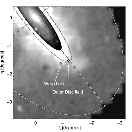
Figure 1: Location of the HST fields (small black squares), overplotted on the surface density of RGB stars from the INT/WFC survey of Irwin et al. (2005) in standard coordinate projection. An optical image of the inner disc has been overlaid. The inner ellipse has a semimajor axis of 2$\degr$ (27 kpc) and represents an inclined disc with $i$ = 77$\aas@@fstack{\circ}$5 and position angle of 38$\aas@@fstack{\circ}$1. The outer ellipse, of semimajor axis length 4$\degr$ (55 kpc), roughly indicates the spatial extent of the INT survey.

1 Introduction

Disc-dominated galaxies account for a sizeable fraction of the stellar mass in the Universe (e.g., Gallazzi et al., 2008; van der Wel et al., 2011) and thus understanding their formation and evolution is of prime importance. In the classical picture, a disc galaxy forms from the collapse of a rotating gaseous protogalaxy within the gravitational potential well of a dark matter halo. As the gas cools and settles into a rotationally-supported disc, it can fragment and undergo star formation (e.g., Fall & Efstathiou, 1980). Modern-day studies place these ideas within a cosmological $\Lambda$ cold dark matter context and use ever more advanced simulations to follow the aquisition of mass through mergers with other systems, as well as from the smooth accretion of intergalactic gas.

Despite the unprecedented numerical resolution and the impressive range of gas physics incorporated, simulations have had difficulties successfully reproducing late-type massive spiral galaxies such as the Milky Way and M31 (e.g., Governato et al., 2009; Agertz, Teyssier, & Moore, 2011) and are only now starting to achieve it (Guedes et al., 2011). A key issue is the so-called ‘angular momentum problem’ which leads to overly small, centrally-concentrated stellar discs dominated by large bulges. Proposed solutions generally invoke various forms and degrees of stellar feedback that suppress star formation at early epochs thereby allowing extended discs to form, albeit at relatively recent times (z$<$1). Due to the expected inside-out growth of the disc, such models require young mean stellar ages at large radii and interesting constraints arise from observations of old and intermediate age stars in these parts (e.g., Ferguson & Johnson, 2001; Wyse, 2008).

Once in place, various processes may influence the star formation and chemical enrichment history of galactic discs. Near or long-range interactions with neighbouring galaxies can redistribute gas and stars and trigger bursts of star formation in which significant fractions of the total stellar mass can form (e.g., Di Matteo et al., 2008; Wong et al., 2011). Various authors have also shown how stars can undergo large radial excursions due to scattering off recurrent transient spirals and other features (e.g., Sellwood & Binney, 2002; Roškar et al., 2008a; Minchev et al., 2011) as well as to perturbations caused by satellite accretion (Bird, Kazantzidis, & Weinberg, 2011). The primary effect is to efficiently mix stars over kiloparsec scales within discs, the consequences of which could be quite profound. For example, if considerable radial migration takes place in discs, it would pose a severe problem for interpreting analyses of the resolved fossil record since the current location of an old star may be far removed from its actual birth place (Roškar et al., 2008b). However, as of yet, there is little direct and unambiguous observational evidence for radial migration (e.g., Haywood, 2008).

Table 1: Summary of Observations

Field	Warp	Outer Disc
R.A. (J2000)	00:38:05.1	00:36:38.3
Decl. (J2000)	+39:37:55	+39:43:26
$R_{proj}$ (kpc)	25.4	26.4
$R_{disk}$ (kpc)	31.5	26.4
E(B$-$V)	0.054	0.055
Dates	2003 Jun 9$-$12	2003 Aug 13$-$16
tF606W (s)	8$\times$1310=10480	8$\times$1250=10000
tF814W (s)	4$\times$1250+8$\times$1330=15640	4$\times$1200+8$\times$1280=15040

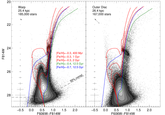
Figure 2: Color-magnitude diagrams for the Warp (left) and Outer Disc (right) fields, where selected isochrones and a ZAHB from the BaSTI library (Pietrinferni et al., 2004) are overlaid. The error bars show the mean photometric errors as a function of magnitude. In each panel, the projected radial distances and the number of stars in the CMDs are indicated. The contour levels correspond to [30, 55, 80, 105, 130, 155, 180]$\times 10^{3}{\rm\ stars\ mag}^{-2}$. The 50% completeness limit from the artificial stars tests (see Section 2.4) is also shown by the dashed line in the left panel. The arrows in the top left of each panel indicate the amplitude of reddening (black arrows, from Schlegel, Finkbeiner, & Davis, 1998) and differential reddening (gray arrow, see Section 4). Note the large spread in the features of the Outer Disc field due to strong differential reddening.

The best place to test ideas about disc formation and evolution is in the nearest external systems where stellar populations with a broad range of age, including those formed at cosmologically-interesting epochs (z$\sim$1–2), can be resolved into individual stars. There has been remarkable recent progress in this field, thanks largely to the ANGST and LCID collaborations which have obtained high-quality Hubble Space Telescope (HST) observations of resolved populations in a variety of nearby galaxies (e.g., Bernard et al., 2009; Dalcanton et al., 2009; Williams et al., 2009a; Monelli et al., 2010; Hidalgo et al., 2011). Of particular importance are studies of populations in the outermost regions of spiral discs: although these regions contain only a minor fraction of the total disc mass, they are where many evolutionary models diverge the most in their predictions and are therefore most easily tested. Interestingly, while the star formation histories (SFHs) reported thus far show evidence of inside-out disc growth (e.g., Williams et al., 2009b, 2010; Gogarten et al., 2010; Barker et al., 2011), they also indicate that a significant fraction of the mass in discs was in place by z$\sim$1–2.

Over the past few decades, HST color-magnitude diagrams (CMDs) of the outer regions of the our largest Local Group neighbours, M31 and M33, have been obtained and analysed in the context of their SFHs. Some of these observations have been limited in depth (Williams, 2002) while others have had their interpretations complicated by the presence of multiple structural components and/or halo substructure (Brown et al., 2006; Barker et al., 2007; Richardson et al., 2008; Richardson, 2010). Studies of fields sampling the entire M33 disc have revealed a clear detection of an inverse age gradient which reverses across the disc truncation (Williams et al., 2009b; Barker et al., 2011). During Cycle 11, 47 HST orbits were dedicated to observe eleven fields in the outskirts of M31 with the Advanced Camera for Surveys (ACS; P.ID. 9458, P.I.: A. Ferguson). Two outer disc fields were observed for ten orbits each, while three orbits were secured for each of the remaining halo substructure fields. The analysis of the stellar populations of the substructure based on this dataset has been presented in an earlier series of papers. Ferguson et al. (2005) explored the stellar populations associated with five prominent stellar overdensities in the halo of M31, and found large-scale population inhomogeneities in terms of age and metallicity. A more in-depth analysis of one of these fields, the G1 Clump, placed constraints on the SFH of this region and noted the similarity to the M31 outer disc population (Faria et al., 2007). Finally, Richardson et al. (2008) combined this dataset with other deep archival datasets in order to explore the nature and origin of the substructure. The global picture that emerges from their homogeneous analysis of 14 HST CMDs is that the substructure can be largely explained as either stripped material from the Giant Stellar Stream progenitor (Ibata et al., 2001) or material torn off from the thin disc through disruption.

Here, we focus on the analysis of the two deep disc pointings sampling the Warp and Outer Disc. While the Warp field was previously presented in Richardson et al. (2008), it was analysed at a only fraction of its total depth (three out of the ten orbits) and the observations presented here are roughly a full magnitude deeper. The paper is structured as follows: in Section 2, we describe the observations and data reduction, and present the resulting CMDs. The CMD-fitting method used to recover the SFH is described in Section 3, along with the results for the Warp field in M31 and the S1 field in M33. In Section 4, the differential reddening affecting the CMD of the Outer Disc field is measured, and used to constrain the fine-scale distribution of dust in the field. The multi-epoch nature of the datasets allowed us to search for variable stars in both fields; they are briefly described in Section 5. Our interpretation of the results is discussed in Section 6 and a summary of the main results is given in Section 7.

2 The Data

2.1 Observations

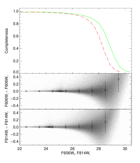
Figure 3: Results from the artificial star tests for the Warp field. Top: Completeness in the F606W (green, solid line) and F814W (red, dashed line) bands as a function of injected magnitude. Middle (bottom) panel: residuals between injected and recovered F606W (F814W) magnitudes as a function of injected magnitude. The crosses and lines indicate the median and standard deviation of the residuals calculated in 1 mag bins.

The two disc fields have been observed with the Advanced Camera for Surveys onboard the HST. Their location was chosen so that the on- and off-axis stellar populations could be sampled and compared. Throughout this paper, we assume a distance of 783 kpc, corresponding to (m$-$M)₀=24.47 (Holland, 1998), and an inclined disc with P.A. = 38$\aas@@fstack{\circ}$1 (Ferguson et al., 2002) and $i$ = 77$\aas@@fstack{\circ}$5 (Ma, Peng, & Gu, 1997). Located $\sim$18$\arcmin$ apart, the $`$Outer Disc’ field samples the outer HI disc along the major axis at projected (deprojected) radius of $\sim 26$ (26) kpc, while the $`$Warp’ field samples the stellar disc at a projected (deprojected) radius of $\sim 25$ (31) kpc, where it strongly bends away from the major axis. Note that the deprojected radii, which correspond to circular radii within the disc plane, are only valid in the case of a planar disc, which is clearly not true in the outer regions of M31. Assuming a dust-free exponential disc scalelength of $\rm{R}_{d}=5.3\pm 0.5\ \rm{kpc}$ (Courteau et al., 2011), these radii correspond to $\sim$5–6 scalelengths.

The fields are shown in Figure 1, overplotted on a map of the surface density of RGB stars from the INT/WFC survey of Irwin et al. (2005). For each field, 8 and 12 images were secured in the F606W and F814W bands during about four consecutive days. Exposure times of $\sim$1,300 seconds per exposure lead to a total of about 10,000 and 15,000 seconds in F606W and F814W, respectively. A detailed summary of observations including coordinates, foreground color excess, projected and deprojected radial distances, and exposure times is given in Table  1.

2.2 Photometry and Calibration

The pipeline processed, non-drizzled (‘FLT’) data products were retrieved from the archive and each exposure was split into two individual images corresponding to the two ACS chips. Additional processing to correct for intra-field variations of the pixel areas on the sky and to flag bad pixels was done using the pixel area maps and data quality masks, respectively. Stellar photometry was carried out with the standard DAOPHOT/ALLSTAR/ALLFRAME suite of programs (Stetson, 1994) as follows. We performed a first source detection at the 3-$\sigma$ level on the individual images, which was used as input for aperture photometry. From this catalog, 300 bright, non-saturated stars per image were initially selected as potential PSF stars. An automatic rejection based on the shape parameters was used to clean the lists, followed by a visual inspection of all the stars to remove the remaining unreliable stars. We ended up with clean lists containing at least 200 good PSF stars per image. Modelling of the empirical PSF with a radius of 10 pixels (0.5$\arcsec$) was done iteratively with DAOPHOT: the clean lists were used to remove all the stars from the images except PSF stars, so that accurate PSFs could be created from non-crowded stars. At each iteration, the PSF was modeled more accurately and thus the neighbouring stars removed better. Every 3 to 5 iterations, the degree of PSF variability across the image was also increased, from constant to linear, then quadratically variable.

The following step consisted of profile-fitting photometry on individual images using ALLSTAR with the empirical PSFs previously created. The resulting catalogs were used to calculate the geometric transformations between the individual images using DAOMATCH/DAOMASTER. From these transformations, it was possible to create a median, master image by stacking all the images from both bands using the stand-alone program MONTAGE2. This master image, clean of cosmic rays and bad columns and much deeper than any individual frame, was used to create the input star list for ALLFRAME by performing a second source detection.

The output of ALLFRAME consists of a catalog of PSF photometry for each image. A robust mean magnitude was obtained for each star by combining these files with DAOMASTER, keeping only the stars for which the PSF fitting converged in at least (N_i/2)+1 images per band, where N_i represents the total number of images per band. This constraint greatly limits the number of false detections due to noise at faint magnitudes.

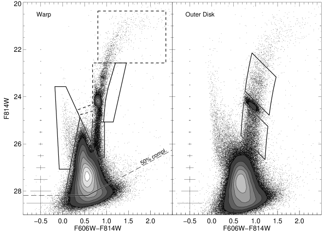
Figure 4: Color-magnitude diagrams for the Warp and Outer Disc fields showing the location of the regions used for the CMD-fitting (left) and for estimating the differential reddening (right, see Section 4). In the left panel, the dashed boxes indicate the location of the two additional bundles used to test our SFH calculation (see Figure 14).

The final photometry was calibrated to the VEGAMAG system following the prescriptions of Sirianni et al. (2005), with the revised ACS zeropoints. Note that the CMD-fitting technique used in this paper minimizes the impact of the uncertainties in distance, mean reddening, and photometric zero-points on the solutions by shifting the observed CMD with respect to the artificial CMD; therefore, any small errors in these quantities do not affect the results.

2.3 Color-Magnitude Diagrams

Figure 2 shows the CMDs for the Warp (left) and Outer Disc (right) fields. These were cleaned of non-stellar objects using the photometric parameters given by ALLFRAME, namely $\sigma_{606,814}\leq$ 0.3 and $-$0.3 $\leq$ SHARP $\leq$ 0.3. Selected isochrones from the BaSTI library (Pietrinferni et al., 2004) are shown, both to indicate the location of the oldest main-sequence turn-offs (MSTO) and as a guide for comparing the two CMDs. As already noted by Richardson et al. (2008), the horizontal-branch (HB) of the Warp field is very sparsely populated. A theoretical zero-age horizontal-branch (ZAHB) for [Fe/H]=$-$0.7 from the same stellar evolution library is overplotted to show its expected location. The reddening (black arrows, from Schlegel, Finkbeiner, & Davis, 1998) and differential reddening (gray arrow, see Section 4) at these locations are also shown in the top left of each panel.

Despite their apparent proximity to each other in the south-western part of the disc, the CMDs of the two fields present notable differences. While the main sequence (MS) of the Warp field contains very few stars younger than $\sim 250-300$ Myr, the Outer Disc field harbors stars as young as a few tens of million years. On the other hand, a plume of stars at 0.3 $\leq$ F606W$-$F814W $\leq$ 0.6 and F814W $\ga$ 25.5, indicative of strong star formation until about 1 Gyr ago, is far more prominent on the CMD of the Warp field.

Concerning the evolved stages of evolution, both fields exhibit well-populated red giant branch (RGB) and red clump (RC) features. There are also hints of AGB bumps at F814W$\sim$23.2. The Outer Disc RGB has a much larger color dispersion than that of the Warp, and the fact this spread is along the direction of the reddening vector, especially apparent from the morphology of the red clump (RC), indicates that the field is strongly affected by differential reddening. We will discuss and quantify this reddening in Section 4.

Finally, the photometry of the Warp field is about 0.3 mag shallower than that of the Outer Disc field. This is mainly due to the higher background at the time of observation.

2.4 Artificial Star Tests

In order to retrieve an accurate SFH from a CMD, a good knowledge of the external factors affecting the photometry is necessary. This is usually done through extensive artificial star tests, whereby a large number of artificial stars are added to the original images, and the photometry is repeated exactly the same way as for the real stars. The comparison between the injected and recovered magnitudes reveals the biases due to observational effects, such as signal to noise limitations, stellar crowding, and blending, as well as quantifies the completeness of the photometry.

Unfortunately, these tests cannot quantify the effect of differential reddening, as observed in the Outer Disc field and described in the previous section. In this particular case, the variations are so strong that the CMD-fitting technique used to recover the SFH described in Section 3 would be in vain. Hence, the artificial star tests were only performed on the images of the Warp field.

The list of stars added to the images was produced by IAC-star (Aparicio & Gallart, 2004). It consists of a synthetic CMD with very wide ranges of ages (0–15 Gyr) and metallicities (Z=0.0001–0.02) in order to cover larger ranges of color and magnitude than for the observed stars. The stars were added on a triangular grid, separated by 20 pixels (twice the PSF radius), to avoid overlap between the artificial stars and optimally sample the whole field of view. Twenty iterations per image, each with 24,395 artificial stars, were necessary to obtain a sufficient sampling of the parameter space. In total, almost a million unique artificial stars were added to the images for these tests.

Figure 3 presents the results of the artificial star tests. The top panel shows the completeness as a function of magnitude for each band. For the F606W and F814W bands, the photometry is 90% complete down to 27.29 and 26.85 mag, respectively, but drops to 50% at F606W=28.75 and F814W=28.18. As shown in Figure 2, this latter limit roughly corresponds to the magnitude of a 12.5 Gyr old MSTO. The middle and bottom panels of Figure 3 compare the injected and recovered magnitudes of the artificial stars in each band, as a function of injected magnitudes. The offset toward positive residuals at fainter magnitudes is a consequence of crowding in these fields, which causes stars to be recovered brighter than the input magnitudes.

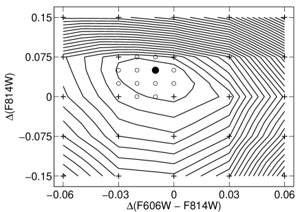
Figure 5: Summary of the 888 calculated solutions in the color-magnitude plane: 24 solutions were calculated at each location indicated by a plus symbol or a circle. The contours show the resulting $\chi^{2}$ distribution in steps of 0.5. Our best-fit solution is the average of the 24 solutions indicated by the filled circle.

3 Quantitative Star Formation History of the Warp Field

3.1 Method

The SFH of the Warp field in M31 was derived through the widely-used CMD-fitting technique, in which the observed CMD is compared with synthetic CMDs created using up-to-date models of stellar evolution. In particular, we adopt the IAC method developed for the LCID Project (e.g., Monelli et al., 2010), which uses IAC-star (Aparicio & Gallart, 2004) to generate synthetic populations, IAC-pop (Aparicio & Hidalgo, 2009) to find the best solution, and MinnIAC (Hidalgo et al., 2011) to produce the input files for, and process the output files from, IAC-pop.

The comparison between the observed and synthetic CMDs is done by simply counting the number of stars in specific areas – referred to as $`$bundles’ (Aparicio & Hidalgo, 2009) – of the CMDs. These areas are chosen on the basis of reliability through considering observational effects (e.g., signal-to-noise ratio, stellar density) as well as theoretical uncertainties in stellar evolution models. To limit the effects of the former, we only consider stars on the CMD brighter than the 50% completeness level in both bands. We also exclude stars on the red giant branch brighter than F814W$\sim$25 (i.e., one magnitude below the RC). The choice to exclude the latter is mainly motivated by the confusion between the various phases of stellar evolution in this part of the CMD – RGB, asymptotic giant branch, RC, red HB, and red supergiant branch – as well as the uncertainties in the theoretical models of these advanced evolutionary stages (see, e.g., Skillman et al., 2003; Gallart, Zoccali, & Aparicio, 2005; Williams et al., 2009a). Indeed, most SFH analyses that are based on deep MSTO photometry do not include this part of the CMD in the fitting procedure (e.g., Brown et al., 2006; Monelli et al., 2010; Hidalgo et al., 2011) although our tests reveal that this does not have a very strong effect on the resultant solution (see Figure 14, and Barker et al., 2011). The bundles used for the Warp CMD are shown as solid lines in the left panel of Figure 4.

The bundles are divided uniformly into small boxes, the size of which depends on the density of stars and reliability of the stellar evolution models. The size of these boxes ranges from 0.06$\times$0.04 mag for the bundles covering the MS to 0.3$\times$0.5 for the bundle located on the red side of the RGB. This yields a total number of $\sim 10^{3}$ boxes. Since every box carries the same weight, the much larger number of boxes on the MS also gives a higher weight to this well-understood evolutionary phase in the SFH calculations.

The number of observed stars, and artificial stars from each simple stellar population (SSP), counted in each CMD box serves as the only input to IAC-pop. IAC-pop then tries to reproduce the observed CMD as a linear combination of synthetic CMDs corresponding to SSPs, that is, populations with small ranges of age and metallicity. No a priori age–metallicity relation, or constraint thereon, is adopted: IAC-pop therefore solves for both ages and metallicities simultaneously. The goodness of the coefficients in the linear combination is measured through the $\chi^{2}$ merit function, which IAC-pop minimizes using a genetic algorithm. These coefficients are directly proportional to the star formation rate of their corresponding SSPs.

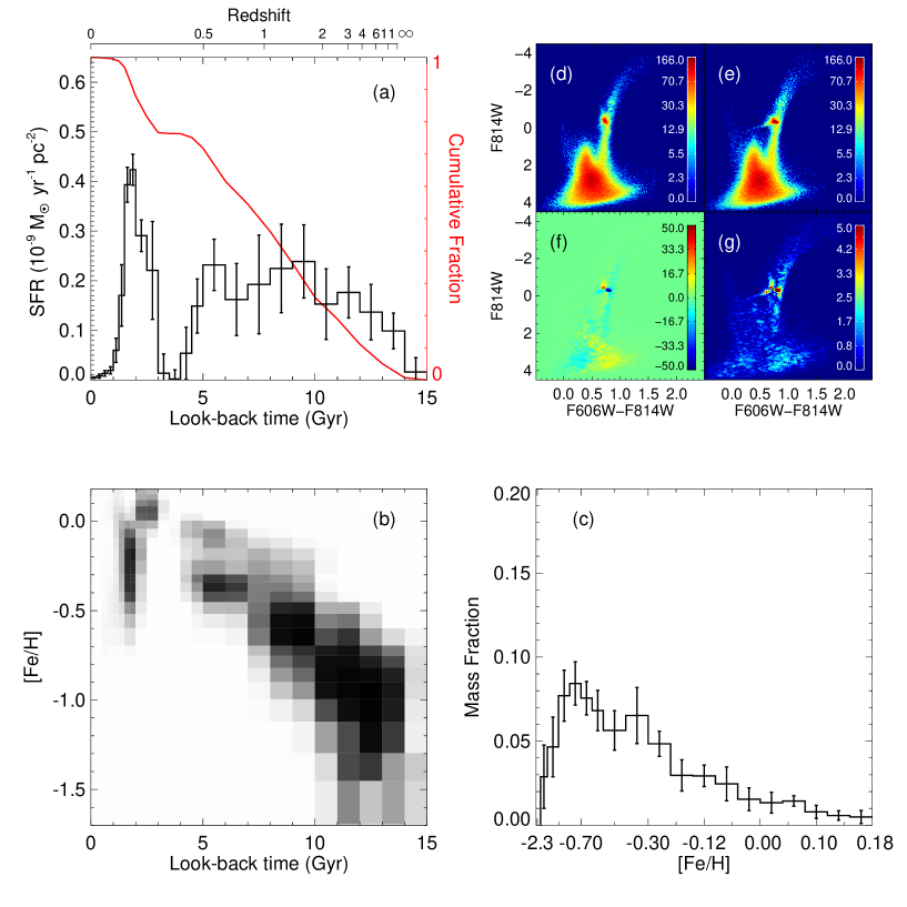
Figure 6: Best-fit SFH solution for the Warp field, obtained with the BaSTI library. The panels show: (a) the SFR as a function of time, normalised to the deprojected area of the ACS field, (b) the age-metallicity relation, (c) the metallicity distribution of the mass of stars formed, (d)-(e) the Hess diagrams of the observed and best-fit model CMDs, (f) the residuals, and (g) the significance of the residuals in Poisson $\sigma$. The cumulative mass fraction is shown in red in panel (a). See text for details.

Age and metallicity are not the only parameters that can influence the best-fit solution. Uncertainties in the distance, mean reddening, photometric zero-points and model systematics, as well as the subjective selection of CMD areas and definition of the SSPs, also affect the resulting SFH solution. MinnIAC was specifically developed to explore this vast parameter space and combine the best solutions at each gridpoint to obtain a robust, stable overall SFH. Its two main purposes are: i) to automate the production of the input files to run a large number of IAC-pop processes in order to sample the whole parameter space, and ii) to average all the solutions obtained at a given distance and reddening to reduce the impact of any specific choices.

We generated a synthetic CMD containing 10⁷ stars using IAC-star (Aparicio & Gallart, 2004) with the following main ingredients. We select the BaSTI stellar evolution library (Pietrinferni et al., 2004), more specifically the scaled-solar models with overshooting, within age and metallicity ranges of 0 to 15 Gyr old and 0.0004$\leq\rm{Z}\leq$0.03 (i.e., $-$1.7$\leq$[Fe/H]$\leq$0.18 assuming $Z_{\sun}=\rm{0.0198}$; Grevesse & Noels 1993), respectively. We assume the Kroupa (2002) initial mass function (IMF), which is a broken power law with exponents of $-$1.3 for stars with masses $<0.5\rm{M}_{\sun}$ and $-$2.3 for higher masses. Hidalgo et al. (2011) carried out extensive tests of the effect of different IMF slopes for their IC1613 and LGS3 analysis, and found the best results were obtained with values compatible with the Kroupa IMF. They did note, however, that the resulting SFH was rather insensitive to realistic changes of the IMF slope. In addition, since our data do not reach the lower mass range, a different choice of IMF slope only affects the normalization and not the relative star formation rates (SFRs; see also Brown et al., 2006; Barker et al., 2007). Finally, the binary fraction and mass ratio were set to f=0.5 and q$>$0.5, respectively, which is in agreement with G and M star surveys of the Milky Way field population (e.g., Duquennoy & Mayor, 1991; Reid & Gizis, 1997). According to the tests performed by Monelli et al. (2010) on five galaxies, the binary fraction only marginally affects the derived SFHs.

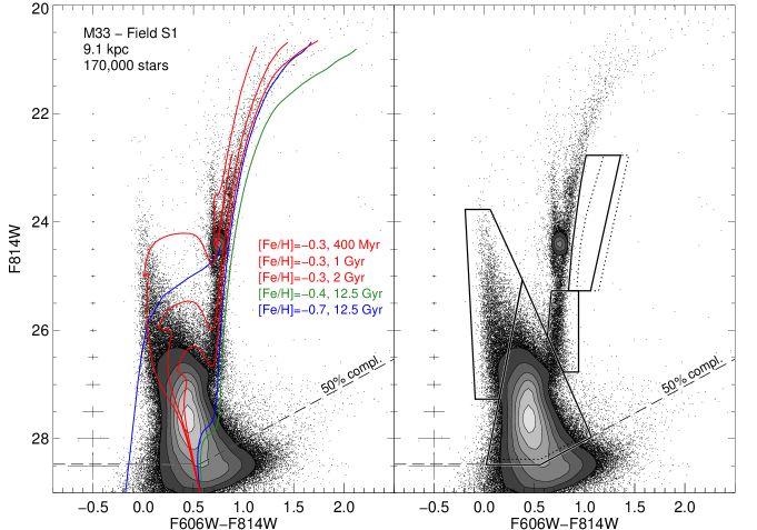
Figure 7: Color-magnitude diagram for the reprocessed M33 field S1 from Barker et al. (2011), where the deprojected radial distance and the number of stars in the CMD are indicated. The contour levels, isochrones, and ZAHB are the same as in the left panel of Figure 2 to facilitate comparison. The 50% completeness limit from the artificial stars tests is also shown by the dashed line. Right: same as left panel, only showing the location of the four bundles used for the SFH calculations. The dotted lines show the bundles used for M31, shifted to the distance and reddening of M33.

As a first step, the age–metallicity plane was divided in 19 age bins and 10 metallicity bins, producing the equivalent of 190 SSPs. The choice of bin sizes ($\Delta$(age): 0.5 Gyr between 0 and 4 Gyr old, 1 Gyr beyond; metallicity boundaries at Z=[0.0004 0.0007 0.0010 0.0020 0.0040 0.0070 0.0100 0.0150 0.0200 0.0250 0.0300]) was made after testing various combinations. However, as stated above, the exact choice of these simple populations can affect the solution, so the SFH was calculated several times, each time slightly shifting the age and metallicity limits of each bin, as well as the location of the boxes on the CMDs in which stars are counted. As was done for the LCID Project, the age and metallicity bins were shifted three times, each time by an amount equal to 30% of the bin size, with four different configurations: (1) moving the age bin toward increasing age at fixed metallicity, (2) moving the metallicity bin toward increasing metallicity at fixed age, (3) moving both bins toward increasing values, and (4) moving toward decreasing age and increasing metallicity. These twelve different sets of parameterization were used twice, shifting the boxes a fraction of their size across the CMD. These 24 individual solutions were then averaged to obtain a more stable solution. The $\chi^{2}$ of this average solution is simply the average of the 24 individual reduced $\chi^{2}$, which we denote $\overline{\chi^{2}}$.

This process is then repeated several times after shifting the observed CMD with respect to the synthetic CMDs in order to account for uncertainties in photometric zero-points, distance and mean reddening. Here we shift the CMD 25 times on a regular 5$\times$5 grid within the following limits: $-0.06\leq\Delta(F606W-F814W)\leq 0.06$ and $-0.15\leq\Delta F814W\leq 0.15$, as shown in Figure 5. These limits are roughly twice the uncertainties in reddening and distance, and correspond to $\Delta\rm{E(B-V)}\sim 0.06$ and $\Delta\rm{D}\sim 55$ kpc. Each plus symbol in Figure 5 represents one of the nodes of this grid, where 24 individual solutions were calculated and averaged. This produced a $\chi^{2}$–map where the contours indicate the approximate location of the absolute minimum in the distance–reddening plane. A second series of finer shifts around this minimum was applied to refine its location; these are shown as the 12 circles in Figure 5. Therefore, 888 individual solutions were calculated in total. The filled circle indicates the location of the averaged solution with the lowest reduced $\overline{\chi^{2}}$, i.e., our best-fit solution SFH, with $\overline{\chi^{2}}_{\rm{min}}=3.08$. We stress that we do not consider the position of the best $\overline{\chi^{2}}$ in the distance–reddening map as a reliable estimate of distance or reddening since photometric zero points, model uncertainties, and other hidden systematics will affect its absolute location.

The uncertainties on the SFRs were estimated following the prescriptions of Hidalgo et al. (2011). The total uncertainties are assumed to be a combination of the Gaussian uncertainties $\sigma_{G}$ – which include errors on distance, reddening, and photometric zero points, as well as the effect of sampling in the color–magnitude and age–metallicity planes – and Poissonian uncertainties $\sigma_{P}$, due to the effect of statistical sampling in the observed CMD. Given the large number of solutions calculated after varying the input parameters, the rms deviation of all the ‘good’ solutions can be assumed to be a reliable proxy of $\sigma_{G}$. Defining $\overline{\chi^{2}}_{\rm{min}}$ and $\sigma_{\overline{\chi^{2}}_{\rm{min}}}$ as the lowest reduced $\overline{\chi^{2}}$ and its standard deviation, we consider ‘good’ all the individual solutions with $\chi^{2}\leq\overline{\chi^{2}}_{\rm{min}}+\sigma_{\overline{\chi^{2}}_{\rm{min}}}$, regardless of their location on the $\chi^{2}$–map.

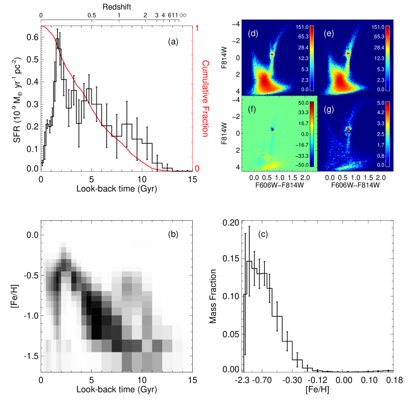
Figure 8: Same as Figure 6, but for the reprocessed M33 field S1 of Barker et al. (2011).

The Poissonian errors are determined by varying the number of stars in each box of the observed CMD according to Poisson statistics, with all the other parameters held fixed, and recalculating the solution. This process is repeated 20 times, and the rms dispersion of these solutions is taken as $\sigma_{P}$. The total uncertainty is the sum in quadrature of $\sigma_{G}$ and $\sigma_{P}$.

To assess the significance and reliability of the SFH solution and to understand the possible systematics, we repeated the calculation of the Warp SFH several times either: i) using the Padova stellar evolution library (Girardi et al., 2000), ii) constraining the range of metallicities for young ages ($<$3.5 Gyr), or iii) including the bright end of the CMD; as well as tried to recover the SFH of a series of artificial CMDs for which the input SFHs were known. The calculations were done strictly following the method described in this section. The results proved very reassuring and are presented and discussed in the Appendix.

3.2 Results

Our best-fit solution SFH is presented in Figure 6. The different panels show: the evolution of the SFR (a) and metallicity (b) as a function of look-back time; (c) the metallicity distribution of the mass of stars formed; (d)-(e) the Hess diagrams of the observed and best-fit model CMDs; (f) the residual differences between the two, in the sense observed$-$model; and (g) the absolute residual difference normalized by Poisson statistics in each bin. The redshift scale shown on panel (a) was constructed assuming the WMAP cosmological parameters from Jarosik et al. (2011): $H_{0}=71.0\ \rm{km}\ \rm{s}^{-1}\ \rm{Mpc}^{-1}$, $\Omega_{\Lambda}=0.73$ and $\Omega_{\rm{M}}=0.27$.

The most striking feature of the SFH shown in Panel (a) is its complexity; it bears little resemblance to the smooth SFHs often invoked in the theoretical models of disc evolution. Star formation in the Warp field began early on and proceeded at a fairly constant rate for the first $\sim$10 Gyr, after which the rate declined rapidly. By that point, roughly 75% of the stars had been formed. Between 4 and 3 Gyr ago, the SFR is consistent with being zero. The following $\sim$1.5 Gyr saw a strong burst of star formation, about twice the intensity of the SFR at earlier epochs, during which the remaining 25% of the stellar mass formed. For comparison, the SFR per unit area of this burst at maximum is about half of the current value in the ‘10 kpc ring’ (Tabatabaei & Berkhuijsen, 2010), the area with the highest current SFR in M31. This burst was followed by a low residual SFR until the present time, responsible for the sparse MS brighter than F814W $\sim$ 26. The derivation of the SFH using the Padova library (see Appendix A) is in excellent overall agreement with that reported here. In particular, both solutions recover a strong burst $\sim 2-3$ Gyr ago, as well a lull in activity $\sim 3-4$ Gyr ago, and the median age of the population, defined as the time at which 50% of the stellar mass was in place, is $\sim$7.5 Gyr in both cases.

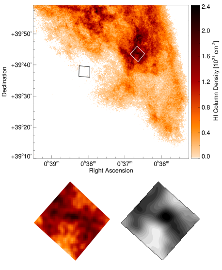
Figure 9: Top: H i column density distribution in the south-west disc of M31, from Braun et al. (2009). The location of the Warp and Outer Disc fields are shown as the small black and white squares, respectively. Bottom: Zoom-in of the Outer Disc field. The H i column density (left), and reddening map derived from the spread of the RGB stars along the reddening vector (right) are shown (see text). The similarity in morphology of the distributions is striking.

The age-metallicity relation (AMR) shown in panel (b) is rather well constrained, increasing smoothly from [Fe/H] $\sim-$1.2 at 13 Gyr to slightly above solar metallicity 2 Gyr ago. From panel (c), the peak metallicity [Fe/H] $\sim-$0.7 is as expected from the morphology of the RGB (see Figure 2), and in excellent agreement with the stellar metallicity measured in other outer disc and halo fields both from photometry (e.g., Reitzel, Guhathakurta, & Rich, 2004; Rich et al., 2004; Ferguson et al., 2005; Brown et al., 2006; Faria et al., 2007; Richardson et al., 2008) and spectroscopy (e.g., Ibata et al., 2005; Collins et al., 2011).

A tantalizing feature in the AMR is the apparent decrease in metallicity from slightly super-solar 2 Gyr ago to [Fe/H]$\sim-$0.3 at the present-day. This behaviour is also recovered in the solution calculated with the Padova stellar evolution library, although not as strong, but it does not appear in any of the tests carried out with mock galaxies (see Appendix A). We explored fits in which the metallicity was constrained to lie within a narrow range at recent epochs but this led to larger residuals (see also Brown et al. (2006) who noted a similar behaviour in their M31 fields). The decline in metallicity in the most recently formed populations therefore appears genuine although it rests entirely on just a few bins. Possible explanations for this behaviour include a scenario in which these stars have been accreted from a low mass galaxy (e.g., a Leo A-type dwarf galaxy; Cole et al., 2007) or that the stars formed in situ from low-metallicity gas which was present in this region $\sim 2$ Gyr ago.

As shown by the Hess diagrams in panels (d)-(g), the model CMD corresponding to this SFH matches very well the observed CMD. The only significant residuals in the difference and significance plots are due to the RC and red HB which, as already discussed, are notoriously difficult features to fit with current stellar evolution models. Note, however, that the stars of the RC and HB have not been used for the calculations of the SFH (see Section 3.1).

3.3 Reprocessing the Barker et al. (2011) M33 data

In an attempt to explain the low surface brightness substructure recently-discovered around M33, McConnachie et al. (2009) explored the interaction between M31 and M33 using a set of realistic self-consistent N-body models. Their favoured orbits bring the systems within $\sim 50$ kpc of each other 2–3 Gyr ago, almost exactly coincident with the major burst of star formation we have found in the Warp field. Barker et al. (2011) recently presented the SFH obtained for a deep HST/ACS field at the edge of the main disc in M33 (R_deproj=9.1 kpc, or about 4 scalelengths) which revealed a star formation enhancement in the past few Gyr similar to that observed in M31. We therefore considered it worthwhile to further investigate the nature and timescale of the M33 burst and examine the evidence that the interaction could have triggered simultaneous star formation episodes. In order to facilitate the most robust comparison, we opted to reanalyse the M33 outer disc data (field S1 from Barker et al. (2011), the dataset for which is fully described in that paper) in the exact same manner as the M31 data presented here. This bypasses the difficulties inherent in the different choices of algorithms, temporal resolution, IMF, and regions of the CMDs to be fit, as well as the representation of the best solution itself. We thus carried out the photometry and artificial stars tests as described in Section 2 for the M33 field and calculated the SFH following the procedure laid out in Section 3.1.

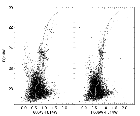
Figure 10: CMDs corresponding to areas of high (left) and low (right) differential internal reddening in the Outer Disc field. Each CMD is drawn from $\sim 10$% of the total area. The same number of stars is plotted in both panels. An old isochrone ([Fe/H]=$-$0.7 and 12.5 Gyr old, from the BaSTI stellar evolution library; Pietrinferni et al. 2004) is overplotted, assuming E(B-V)=0.055 from the map of Schlegel, Finkbeiner, & Davis (1998).

The CMD is shown in Figure 7; the reanalysis of this dataset has led to a gain of an extra $\sim 0.5$ mag in depth over that presented in Barker et al. (2011). Despite being slightly more distant than M31 ($\Delta(\rm{m}-\rm{M})_{0}\sim$ 0.2, Barker et al. (2011)), the somewhat longer exposure times and lower stellar density of the field led to a similar photometric depth and 50% completeness level as for the Warp field. In the left panel, the same isochrones and ZAHB as in Figure 2, shifted to the distance and reddening of M33, have been overplotted for comparison. As already noted by Barker et al. (2011), the oldest MSTO seen in this field is about one magnitude brighter than the 12.5 Gyr old isochrones and therefore significantly younger than the age of the Universe. We assume a distance of 867 kpc (i.e., (m$-$M)₀=24.69; Galleti, Bellazzini, & Ferraro, 2004), inclination of 56$\degr$, position angle of 23$\degr$ (Corbelli & Schneider, 1997), and color excess E(B$-$V)=0.044 as in Barker et al. (2011).

In the right panel we show the bundles used to recover the SFH as thick solid lines. These are virtually the same as the ones used for M31 – shown as the dotted lines, shifted to the distance and reddening of M33. The main difference is the slight shift of the bundle redward of the RGB to bluer colors in order to put tighter constraints on the maximum metallicity.

Our best-fit solution for the outer disc field of M33 is shown in Figure 8. For a more meaningful comparison with the SFH of M31, panel (a) of both Figure 6 and 8 are normalised to the deprojected area taking into account the inclination and morphology of each galaxy. The overall agreement between our solution and that reported in Barker et al. (2011) is excellent: both solutions indicate a dearth of old stars and show that less than half of the total stellar mass was in place before redshift 0.5. The chemical enrichment laws are also very similar, with a mild metal enrichment from [Fe/H] $\sim-$1.0 about 10 Gyr ago to roughly $-$0.5 at the present time, and a median [Fe/H] $\sim-$0.7. We do find a slightly higher SFR around $\sim$8–11 Gyr ago than that reported by Barker et al. (2011) which may result from the increased CMD depth in our reanalysis. This finding is in better agreement with the presence of a few RR Lyrae stars detected in this field (Barker et al., 2011). However, the main difference between the solutions results from the finer temporal grid which we have employed here which allows us to resolve a strong and relatively short burst of star formation which is exactly coeval to that in the Warp field of M31 and has the same duration ($\sim$1.5 Gyr). We note that the drop in metallicity observed in the SFH of the Warp field in M31 at about 2 Gyr ago is also visible in the solution for M33. Together, these findings reinforce the idea that the enhanced SFRs in the outer discs of both galaxies could be related and we discuss this possibility in more detail in Section 6.

4 The Outer Disc Field

As shown in Section 2, the Outer Disc field suffers from significant differential reddening which, by blurring the features along the reddening vector, affects the morphology of its CMD. As we will show below, the dust distribution appears highly complex in this region with some stars lying both in front and behind the dust clouds. Unfortunately, this renders futile attempts to correct for the effects of differential reddening in our data, so the method used in the previous section to recover the SFH of the Warp field can not be applied here. In particular, differential reddening along the RGB mimics the effect of higher metallicity and/or older ages by shifting the stars to the red, thus worsening the age-metallicity degeneracy already present.

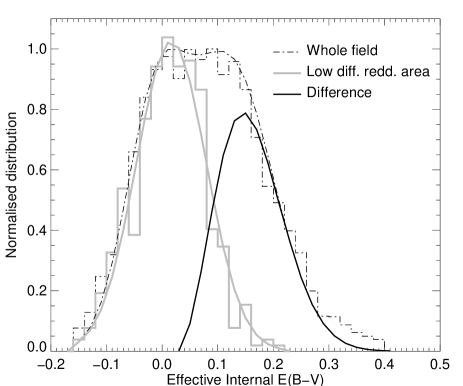
Figure 11: Distribution of effective internal E(B-V) of the Outer Disc field, calculated from the spread of the RGB stars along the reddening vector (see text). Note that this reddening is in addition to the foreground value of 0.055 quoted earlier. Gaussian and double-Gaussian fits to the histograms of the low differential reddening area and the whole field-of-view, respectively, are overplotted. The thick black curve is the difference between these two Gaussian fits.

We focus our analysis of the Outer Disc field on quantifying the amount of differential internal reddening, understanding its origin and constraining the fine-scale distribution of the dust. To estimate the amount of internal reddening as a function of position in the field, we use RGB stars brighter than F814W $\sim$ 26.5, as shown in the right panel of Figure 4, since their distribution along an old isochrone is roughly perpendicular to the reddening vector. This allows us to keep contamination from other stellar evolutionary phases to a minimum. We also exclude stars from the top two magnitudes of the RGB as their color is very sensitive to small changes in metallicity, and age to a lesser extent, as well as the part of the RGB which overlaps the RC.

Given that the blue side of the RGB is well represented by a 12.5 Gyr old isochrone with [Fe/H]=$-$0.7 (see Figure 2), we assume that all RGB stars should have been observed at this location if differential reddening had been negligible. Under this assumption, we can estimate the amount of extinction along the line of sight to a given RGB star by measuring the distance, along the reddening vector, between the star and this isochrone, and convert this distance to an ‘effective internal E(B-V)’. Note that this represents the internal reddening as it is in addition to the foreground value of E(B$-$V)$=0.055$ reported in Table 1 and taken from the map of Schlegel, Finkbeiner, & Davis (1998).

In the bottom right panel of Figure 9 we show the resulting contour map, where darker tones indicate higher extinction. It shows that the distribution of reddening is far from homogeneous in this small field-of-view (FOV) and delineates clumps and filaments with sizes $\la$ a few hundred parsecs. Interestingly, the distribution of reddening is almost an exact match to the morphology of the H i column density map (Braun et al., 2009), kindly supplied by R. Braun and shown in the top and bottom left panels of Figure 9. By comparing the low resolution H i observations of Newton & Emerson (1977) with their photometry, Cuillandre et al. (2001) also found that the colors of the RGB stars were correlated with the column density of H i in their 28$\arcmin\times$28$\arcmin$ outer disc field – which includes our HST field. They concluded that the relatively large amount of extinction is closely associated with the H i gas, and that the outer disc of M31 therefore contains substantial amounts of dust. Our result shows that this interpretation is still valid on the much finer scales sampled here.

From our contour map, we can now select the areas within the FOV where extinction is lowest and highest. We pick stars which fall within two rectangular boxes, each covering roughly 10% of the total area of the ACS FOV. Figure 10 shows the CMDs of these two fields, each containing the same number of stars. The isochrone described above is overplotted in each panel, shifted to the distance of M31 and corrected for foreground reddening. In the left panel, the RGB is very wide, almost bimodal, with a blue RGB nicely fit by the isochrone and a second, redder RGB. The presence of both non- and very reddened stars at the same spatial location indicates a complex 3-dimensional spatial distribution where non-reddened stars possibly lie in front of the dust cloud and the very reddened stars behind. This is precisely why we cannot correct the photometry for differential reddening: applying a correction derived from the contour map of Figure 9 would simply shift the wide RGB to the blue, rather than producing a narrow RGB.

In the right panel of Figure 10, the isochrone provides a good fit to the stars of the lowest differential reddening area, which shows that the differential reddening in this subfield is more limited. For simplicity, we assume in the following that this CMD is representative of the intrinsic spread in color due to a combination of photometric errors and ranges of age and metallicity. However, we note that the lower RGB here is still not as tight as in the Warp field, and thus some differential reddening is still likely to be present if we assume the intermediate-age and old stellar populations to be comparable between the Warp and Outer Disc fields.

Figure 11 shows the normalised distribution of ‘effective internal E(B$-$V)’, as calculated above, for the low differential reddening area (gray histogram) and the whole Outer Disc field (dash-dotted black histogram). Gaussian and double-Gaussian fits to these histograms, respectively, are also shown. The difference between the two therefore represents the additional contribution of the differential reddening to the spread in the CMD, and is shown as the thick black curve in Figure 11. Note that the distribution of E(B$-$V) of the low differential reddening area in Figure 11 is not centred on zero, but is slightly offset by $\sim$0.02. While this might indicate that the foreground reddening taken from the Schlegel, Finkbeiner, & Davis (1998) map at this location is underestimated, it is worth stressing that the values of the ‘effective internal E(B$-$V)’ are only relative to a given isochrone which may not be a perfect representation of the true local reddening. Our goal here is to quantify the differential internal reddening rather than that due to the foreground. The distribution under the thick black curve has a median of $\sim$0.16; subtracting the 0.02 offset, we find that this additional extinction amounts to $\sim$0.14 (corresponding to a total reddening of $\sim 0.2$) and affects about 40% of all the RGB stars.

While we cannot do a detailed SFH reconstruction for the Outer Disc field, we can make an important deduction about the recent SFH from inspection of the high and low reddening CMDs in Figure 10. Neither of these CMDs show evidence for the prominent 1–2 Gyr turn-off population so readily apparent in the Warp CMD hence this region apparently did not undergo a recent burst. Furthermore, the youngest populations ($\sim$ few tens of Myr) are largely confined to the highest reddening regions of the FOV. That such stars are present in the Outer Disc field and not at all in the Warp is not surprising when considering the gas distribution (see Figure 9) which shows that the stellar warp region is currently devoid of high-column density gas.

5 Variable Stars

The candidate variable stars were extracted from the photometric catalogs using the Stetson (1996) variability index $J$, which uses the correlation in brightness change in paired frames to isolate possible variables from constant stars. This process resulted in the selection of $\sim$ 180 and 230 candidates for the Warp and Outer Disc fields, respectively. Most of these turned-out to be false detections, owing their non-zero variability index to the combination of sparse sampling and large numbers of cosmic rays. Inspection of the individual light curves, and the location of the candidates on the stacked images and on the CMDs, allowed us to extract the candidate RR Lyrae stars. The other bona fide variables, mostly eclipsing binary systems, were discarded due to the sparse sampling preventing us from finding their periods. Our final catalog of variable stars contains 12 and 13 RR Lyrae stars from the Warp and Outer Disc fields, respectively. All of these are new discoveries, since no data of sufficient depth or sampling has been obtained before our observations of this part of M31. Interestingly, no Cepheids were detected, despite the presence of young, massive stars in the Outer Disc field.

We performed the period search through Fourier analysis (Horne & Baliunas, 1986), which was then refined by hand to obtain smoother light curves using the same interactive program as described in Bernard et al. (2009). However, the small number of datapoints, as well as an inconvenient temporal sampling (all the images in one band observed consecutively, followed by all the images in the other band) significantly complicated the process. For some variables, several periods could fold our data and give light curves of similar quality. We thus used additional parameters to constrain the most likely period: an amplitude ratio A_F606W/A${}_{F814W}\sim$ 1.8, and a reasonable location on both the period-amplitude diagram and the CMDs. These constraints were determined from the other RR Lyrae stars for which the period search was straightforward. While this may not be ideal for obtaining purely objective periods, the process allowed us to obtain reasonably reliable estimates given the characteristics of the data. It is important to note that some of our final periods could well be aliases of the true period.

Table 2: Properties of the Variable Stars in the Warp field

ID	Type	R.A.	Decl.	Period	$\langle F606W\rangle$	AF606W	$\langle F814W\rangle$	AF814W
		(J2000)	(J2000)	(days)
V01	$c$	00 38 02.64	+39 36 30.9	0.46	26.03	0.35	25.63	0.39
V02	$ab$	00 38 10.16	+39 36 42.8	0.49	25.40	1.25	25.03	0.67
V03	$ab$	00 38 03.65	+39 37 23.9	0.47	24.86	0.65	24.46	0.63
V04	$ab$	00 38 13.85	+39 37 37.0	0.60	25.79	0.71	25.39	0.29
V05	$ab$	00 38 13.53	+39 38 03.9	0.63	25.50	0.69	24.94	0.43
V06	$ab$	00 38 09.02	+39 38 13.8	0.70	25.03	0.81	24.52	0.37
V07	$ab$	00 38 03.12	+39 38 20.3	0.50	25.12	1.44	24.75	0.71
V08	$ab$	00 38 03.05	+39 39 07.5	0.58	25.00	0.79	24.56	0.46
V09	$ab$	00 38 13.77	+39 39 08.2	0.53	24.93	1.18	24.44	0.75
V10	$ab$	00 38 11.26	+39 39 13.3	0.78	24.77	0.41	24.31	0.22
V11	$c$	00 38 11.11	+39 39 14.2	0.305	25.68	0.27	25.12	0.32
V12	$c$	00 38 13.76	+39 39 16.8	0.378	24.92	0.58	24.58	0.27

Table 3: Properties of the Variable Stars in the Outer Disc field

ID	Type	R.A.	Decl.	Period	$\langle F606W\rangle$	AF606W	$\langle F814W\rangle$	AF814W
		(J2000)	(J2000)	(days)
V13	$ab$	00 36 35.63	+39 42 17.0	0.56	25.88	1.01	25.15	0.94
V14	$c$	00 36 34.10	+39 42 27.9	0.269	26.34	0.46	25.76	0.18
V15	$c$	00 36 34.29	+39 43 02.9	0.35	26.25	0.32	25.73	0.33
V16	$ab$	00 36 43.61	+39 43 10.0	0.52	25.07	1.18	24.66	0.77
V17	$c$	00 36 42.00	+39 43 20.4	0.343	25.06	0.40	24.71	0.24
V18	$ab$	00 36 28.25	+39 43 29.9	0.59	24.72	1.03	24.36	0.36
V19	$c$	00 36 36.18	+39 43 40.6	0.35	25.85	0.69	25.30	0.44
V20	$c$	00 36 34.25	+39 43 40.9	0.405	25.91	0.21	25.12	0.23
V21	$c$	00 36 30.60	+39 43 58.5	0.38	25.69	0.51	25.12	0.43
V22	$ab$	00 36 41.28	+39 44 01.9	0.54	25.39	0.55	25.01	0.39
V23	$c$	00 36 44.44	+39 44 41.4	0.39	24.97	0.60	24.62	0.35
V24	$ab$	00 36 42.72	+39 45 10.2	0.452	25.15	1.17	24.88	0.77
V25	$ab$	00 36 40.05	+39 45 48.8	0.51	24.92	1.01	24.54	0.68

Sample light curves for fundamental and first-overtone mode pulsators from each field are shown in Figure 12, where templates from the set of Layden et al. (1999) have been overplotted. Given the difficulty of measuring accurate periods and mean magnitudes, as well as the incompleteness due to the limitations outlined above, we do not attempt to analyse the detailed individual and global properties of these stars. Their locations and approximate properties are given here for future reference.

The properties of the RR Lyrae stars are summarised in Table 2 and 3 for the Warp and Outer Disc fields, respectively. The first and second columns give the identification number and the type of pulsation, with $ab$ and $c$ designating the fundamental (RR$ab$) and first-overtone (RR$c$) mode pulsators, respectively. The discrimination between types was based on the period and light curve morphology. The next two columns contain the equatorial coordinates in J2000.0, while columns (5) lists the period in days. Except in the few cases where a third digit resulted in a significantly smoother light curve (mostly RR$c$), we only give the periods with two significant figures. In the remaining columns, the intensity-averaged mean magnitude, as well as the amplitude of the pulsations, are listed.

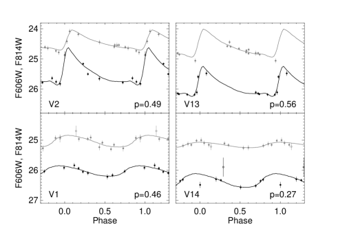
Figure 12: Sample light-curves of two RR$ab$ (top) and two RR$c$ (bottom), taken from the Warp (left) and Outer Disc (right) fields, illustrating the sparse sampling of our data. Black and grey correspond to the F606W and F814W magnitudes, respectively. The star ID is indicated in the lower left and the period in days in the lower right.

The detection of RR Lyrae variables this far out in the disc shows how the variability studies can complement the deep CMD analyses: none of the CMDs presented in this paper harbor the obvious features that are traditionally associated with truly old stellar populations, such as a well-defined faint MSTO or an extended HB. Yet, the characteristic properties of these variables demonstrate that at least some of the stars at F606W-F814W$\sim$0.5 and F814W$\sim$25 belong to an old, extended HB.

6 Discussion

The CMD-fitting technique applied to the Warp field reveals two main episodes of star formation: an extended period of roughly constant star formation over the period from 4.5 to 13 Gyr ago (corresponding to z$\ga 0.5$), and a relatively short-lived burst which peaked $\sim 2$ Gyr ago. In the $\sim$1 Gyr which separates these episodes, very little star formation took place.

The differential reddening present in the Outer Disc field prevents a similar analysis of its SFH. Although we cannot deduce anything about the SFH at early times in this field, the lack of a prominent 1–2 Gyr old MSTO feature in the CMD indicates that it did not experience the same recent burst as seen in the Warp. It is interesting to speculate why the two fields could differ in this respect. Firstly, the disc of M31 is strongly perturbed at large radius and highly inclined with respect to the line of sight. Thus, even though the two pointings appear close in projection on the sky they may actually sample very different radii. If the SFH over the last few Gyr varies strongly as a function of radius in the M31 outer disc, this could explain the different behaviours observed. Furthermore, if the two fields sample different disc radii then they will also have differing levels of contamination from other structural components (e.g. thick disc, stellar halo) which could impact the overall SFHs. There is some evidence that this might be the case from examining published kinematical data for RGB stars in the M31 outer disc. Although not exactly coincident with our ACS fields, fields F1 and F2 from Ibata et al. (2005) are in good proximity to the Outer Disc and Warp pointings respectively. While field F1 shows a single velocity peak with a velocity lag and moderate dispersion ($\sim 30$ km/s), field F2 shows the same component plus a dominant cold component ($\sim 9$km/s) which exactly matches the expected circular velocity of the disc at that location. This suggests that the thin disc may be more dominant in the Warp field than in the Outer Disc field, with the thick disc dominating in the latter.

In what follows, we discuss the two main episodes of star formation in the Warp field separately, assuming that the behaviour observed here is representative of the whole outer thin disc.

6.1 Star Formation at Intermediate and Early Epochs

The star formation rate at lookback times of $\ga 4.5$ Gyr ago (z$\ga 0.5$) is roughly constant and does not show salient features (see Figure 6). While this behaviour may be genuine, it could also (partly) result from the lack of resolution at faint magnitudes (hence old ages) which tends to smooth the resulting SFH (see the tests on mock galaxies in the Appendix as well as the discussion in Hidalgo et al. 2011). One consequence of this smoothing is that some star formation is always recovered in the oldest age bins, even although none may have taken place. Nonetheless, the presence of RR Lyrae stars in the Warp field provides support for a population of stars with age $\ga 10$ Gyr.

If the stars in the Warp field formed in situ, the significant median age of 7.5 Gyr at $\sim 5$ radial scalelengths indicates that M31’s outer disc was in place early on. This argues against a scenario in which M31 underwent a major merger at intermediate epochs after which the disc reformed, as has been recently suggested by Hammer et al. (2010). Other evidence also supports the idea that the outer discs of massive spiral galaxies formed at high redshift (e.g., Ferguson & Johnson, 2001; Brown et al., 2006; Williams et al., 2009a; Muñoz-Mateos et al., 2011). On the other hand, the outer disc of M33 lacks a significant fraction of old stars at 3–4 scalelengths (Williams et al., 2009b; Barker et al., 2011). This could reflect the effect of downsizing within the disc population, whereby stars in more massive discs tend to have formed earlier and over a shorter time-span than in less massive systems (e.g., Cowie et al., 1996). Alternatively, it may simply highlight the uniqueness of M33 – indeed Gogarten et al. (2010) find that the outer disc of the similarily low-mass spiral galaxy NGC 300 is dominated by old stars.

Another interesting feature is the fact that the dominant population which formed at early epochs is relatively metal-rich ([Fe/H]$\ga-$1.3, Figure 6c), at least in the solution obtained with the BaSTI stellar evolution library. This is qualitatively similar to the results of Williams et al. (2009a) for the outer disc of M81, which is to date the only other massive disc galaxy for which the CMD-fitting technique has been applied (although their data do not reach old main-sequence turn-offs). The solutions for their field, located at five scalelengths from the centre of M81, show a constant [M/H] $\sim-$0.5 at all ages. Similarly, our renalysis of the Barker et al. (2011) M33 outer disc field supports the lack of stars with [Fe/H] $\la-$1.5, consistent with their original findings. Therefore, it seems that even the oldest stars in the outer discs of galaxies must have formed from pre-enriched gas.

In the discussion above, we have assumed that the stars which we see today in the outer disc of M31 (and M33) actually formed there. It is possible, however, that these stars formed at much smaller galactocentric distances, where the metallicity was higher at early epochs due to the higher rate of gas recycling, and migrated to their current location due to resonant scattering with transient spiral arms and bars (e.g., Sellwood & Binney, 2002; Roškar et al., 2008a, b; Schönrich & Binney, 2009; Minchev et al., 2011) or other mechanisms (Quillen et al., 2009; Bird, Kazantzidis, & Weinberg, 2011). For example, in the models of Roškar et al. (2008b), roughly 50% of solar neigbourhood stars (i.e. those lying at $\sim 2-3$ scalelengths) have come from elsewhere, with the bulk originating at smaller radii and moving outwards. At extreme radial locations such as we have probed here ($4-6$ scalelengths), this fraction of migrated stars is likely to be even higher on account of the low rate of in situ star formation. Indeed, both M31 and M33 exhibit spiral arm patterns which extend to these large radii, indicating that migration could still be an efficient mechanism for moving stars around. The net effect of radial migration on outer disc stellar populations is to render the SFH and AMR flat and featureless in these parts (see Figure 3 of Roškar et al. (2008b)). This behaviour is in stark contrast to what we see in the Warp and M33 S1 fields, where the SFHs display sharp features, at least back to $\ga$5 Gyr ago, and the AMRs increase smoothly with time from early epochs to 2 Gyr ago. This suggests only a small role for radial migration in populating the M31 and M33 outer discs at the radii we have probed. For the same reasons, it is also unlikely that a significant fraction of the stars in these parts have been directly accreted onto the disc plane from satellite galaxies.

6.2 The 2 Gyr Old Burst

Strong bursts of star formation are often caused by an external trigger such as an accretion event or an interaction with a nearby galaxy (e.g., Kennicutt et al., 1987). Indeed, the copious amount of substructure observed in the outer regions of M31 strongly suggests interactions have taken place (e.g., Ferguson et al., 2002; Richardson et al., 2008; McConnachie et al., 2009).

The well-known giant stream in the south of M31 (Ibata et al., 2001) is the fossil evidence of one such event. It has been modeled rather successfully as either the remnant of a $\sim$$10^{9}M_{\sun}$ satellite accreted less than a billion years ago (e.g., Fardal et al., 2007), or a major merger in which the interaction and fusion with M31 may have started $\sim 9$ and 5.5 Gyr ago, respectively (Hammer et al., 2010). Neither of these scenarios can account for a star formation burst that occured about 2 Gyr ago in the Warp field.

Another possibility is that the close passage of M33 could have triggered star formation on large scales in M31. Using realistic self-consistent N-body simulations, McConnachie et al. (2009) were able to best reproduce the morphology of the outer substructure in M33 with orbits that brought the systems within $\sim$50 kpc of each other 2–3 Gyr ago and that satisfy their current positions, distances, radial velocities, and M33’s proper motion. In particular, they found that M33 reached pericenter about 2.6 Gyr ago, which is in excellent agreement with the start of the star formation bursts observed in Figures 6 and 8. This is highly suggestive of an interaction between the two systems triggering inward flows of metal-poor gas which fuelled moderate bursts of star formation. Such behaviour is consistent with the predictions of state-of-the-art simulations of galaxy interactions and mergers, even though most work to date has focused on the inflow of gas to the central regions (e.g., Di Matteo et al. 2008, Teyssier, Chapon, & Bournaud, 2010).

Further development of these N-body models (Dubinski et al.  in preparation) indicates that the gravitational interaction of M33 should have induced perturbations in M31 in the form of heating and disruption of the outer disc. This is consistent with the presence of warps in both the H i and stellar discs, and the disc-like stellar populations found in many regions of substructure (Ferguson et al., 2005; Faria et al., 2007; Richardson et al., 2008). Such an interaction could also help explain the large fraction of globular-like clusters younger than 2 Gyr in M31 (Fan, de Grijs, & Zhou, 2010), the enhanced SFR 2–4 Gyr ago observed in all the deep HST fields in M33 (Barker et al., 2007; Williams et al., 2009b; Barker et al., 2011), and the warps in both the H i (e.g., Wright et al., 1972; Putman et al., 2009) and stellar discs (McConnachie et al., 2010) of M33. To put this interpretation on firmer footing, additional data are required to assess just how widespread the $\sim$2 Gyr burst of star formation is in the M31 outer disc and address how the timing and intensity of the burst varies with location.

7 Conclusions

We have presented the analysis of very deep, multi-epoch HST data for two fields located in the far outer disc of M31 at $\sim 2\degr$ (26 kpc) from the centre, corresponding to 5–6 radial scalelengths.

We apply the CMD-fitting technique to the Warp field, and find that a significant fraction of the stellar mass ($\sim$25%) was produced as the result of a strong and relatively short-lived burst of star formation about 2 Gyr ago. The re-analysis of the M33 outer disc S1 field of Barker et al. (2011) and resulting SFH show a similar burst of SF that is exactly coeval with that observed in M31. The burst in both galaxies is also accompanied by a decline in global metallicity, which suggests an inflow of metal-poor gas into the outer disc. These results further support the inference from N-body modelling that M31 and M33 had a close interaction about 2–3 Gyr ago that enhanced the outer disc SF at that epoch, and may also be responsible for the warps in the H i and stellar discs of both galaxies and the large fraction of clusters younger than about 2 Gyr old.

Further back, the SFH was roughly constant over the period spanning 4.5–13 Gyr. The presence of stars older than about 10 Gyr, while surprising at such a large distance from the nucleus, is confirmed by the detection of RR Lyrae stars in this field. In addition, the sharp features in the SFH and the rather well-defined and monotonically increasing AMR favour the in situ formation of these stars, rather than an outward migration from birthplaces at much smaller galactocentric radii. The fact that the oldest populations are still fairly metal-rich ([Fe/H]$\ga-$1.3) suggests pre-enrichment of the outer disc material.

The second field, the Outer Disc field, is strongly affected by differential reddening which prevents us from applying the CMD-fitting technique. However, the pattern of reddening inferred from the color of the RGB stars is highly correlated with the H i distribution in the outer disc, suggesting these clouds contain substantial dust indicative of significant metal enrichment. This confirms earlier work by Cuillandre et al. (2001) but goes further in demonstrating how highly structured the dust distribution is on small scales. The presence of significant reddening in these parts is consistent with the roughly solar metallicity in the past few Gyr uncovered by our SFH analysis of the nearby Warp field.

Finally, from a time-series analysis, we find a dozen RR Lyrae stars in each of the two fields. The detection of these variables supports the presence of truly old stellar populations in the far outer discs of galaxies despite the lack of obvious HBs in the CMDs, and shows how variability studies can complement deep SFH analyses.

Appendix A Testing the SFH Calculation Method

Here we describe a series of tests aimed at understanding how reliable the CMD-fitting technique used in this paper is, given the photometric properties of our dataset (i.e., depth, crowding), as well as revealing possible biases and limitations of the method.

The first test consisted of recovering the SFH of the Warp field in the exact same way as described in Section 3, albeit using the stellar evolution library of the Padova group (Girardi et al., 2000). The resulting SFH is shown in Figure 13. The agreement with the SFH obtained with BaSTI (see Figure 6) is excellent. The main features such as the burst centered on 2 Gyr old, the very low star formation between 3–4 Gyr and the smooth increase of metallicity from the earliest epochs to 2 Gyr ago are virtually the same as with the BaSTI library, and the recent decrease in metallicity is also observed, albeit not as strongly. The main difference lies in the overall metallicity, which appears systematically lower by roughly 0.2 dex in the former solution at any age. The sense and amount of this offset is exactly the same as reported in Barker et al. (2011), and is likely due to the difference in color of the RGB between the two libraries (e.g., Gallart, Zoccali, & Aparicio, 2005). We note that the SFH obtained by Brown et al. (2006) with the Victoria–Regina isochrones (VandenBerg, Bergbusch, & Dowler, 2006) for another outer disc field in M31 shows very few stars with metallicity lower than about [Fe/H]=$-$1, which is more in line with the SFH we obtained with BaSTI and agree with spectroscopic estimates of outer disc metallicities in the literature (Ibata et al., 2005; Collins et al., 2011). Another difference between the solutions is that the star formation which occurred earlier than 5 Gyr is not as uniform in the Padova solution as in the BaSTI one, but shows a mild decrease about 8–9 Gyr ago. Given the larger errorbars in the solution obtained with the Padova library, however, we do not consider this feature to be very significant.

For the second test we repeat the fit of the Warp CMD with the BaSTI library, but this time including the evolved stars – as shown by the dashed bundles in Figure 4. The solution presented in Figure 14 is qualitatively similar but the fit is significantly worse ($\overline{\chi^{2}}$=5.27). This is evidenced by the significant residuals in the main-sequence shown in panels (f) and (g). We believe the simultaneous fit of all the features of the CMD produces worse results due to the larger uncertainties in the stellar evolution models of the evolved stars.

The remaining tests involve ‘mock galaxies’ for which CMDs were produced using IAC-star (Aparicio & Gallart, 2004) and invoked SFHs representative of the typical range seen within the Local Group. Observational effects were simulated using the results of the artificial stars tests described in Section 2.4. Figure 15 shows the simplest possible SFH, that of a constant rate between 14 Gyr ago and the present time without chemical enrichment. In panel (a), the input SFH is represented by the green lines, while the recovered SFH is shown as in the previous figure. In panel (b) the two green lines show the upper and lower limits of the input metallicity range, between which the stars were uniformly distributed in each age bin. Ideally, discrepancies between the input and recovered SFH should be representative of the effects of the observational effects and age-metallicity degeneracy.

Finally, for the remaining two mock galaxies, we test the capacity to recover the SFH of a predominantly old galaxy similar to the transitional dIrr/dSph of the Local Group (e.g., LGS3: Hidalgo et al., 2011), and of a mostly young and intermediate-age galaxy like the dwarf irregular Leo A (Cole et al., 2007), both with a mild chemical enrichment over the past 14 Gyr. The results are shown in Figure 16 and 17.

Overall, the SFHs are recovered very well in all cases. Not only are the residuals in the CMDs very low, but the SFRs and metallicities are very close to the input values. In addition, the AMR is measured correctly, which highlights the ability of the method to solve for both age and metallicity simultaneously. There are small discrepancies however, which appear to be systematic:

• while the correct mean metallicity at a given age is usually recovered, the dispersion of metallicity is often overestimated, in the sense that stars are recovered outside the range delineated by the green lines in panel (b) of Figures 15 to 17;

• this effect is strongest for the most recent SFH ($\la$1 Gyr) since metallicity only has a small effect on the color of the bright main sequence and is therefore largely unconstrained;

• the ages recovered for the oldest populations ($\ga$10 Gyr old) are slightly overestimated. This may in fact be revealing the loss of temporal resolution beyond 7–8 Gyr old due to photometric uncertainties at faint magnitudes, as illustrated by the burst of Figure 16 being recovered with a lower amplitude and more spread out in time.

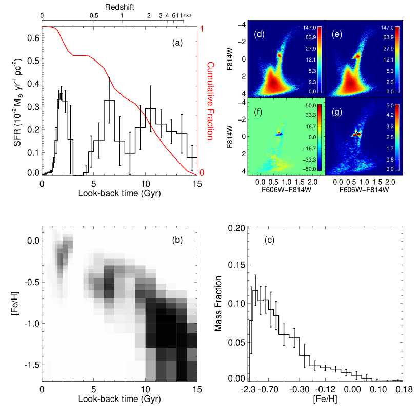
Figure 13: Same as Figure 6, but recovered with the Padova stellar evolution library.

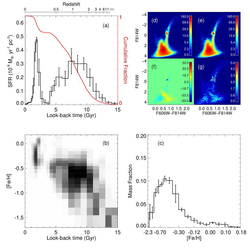
Figure 14: Same as Figure 6, but using two additional bundles to include the RGB, RC, and HB in the fitting, as shown in Figure 4.

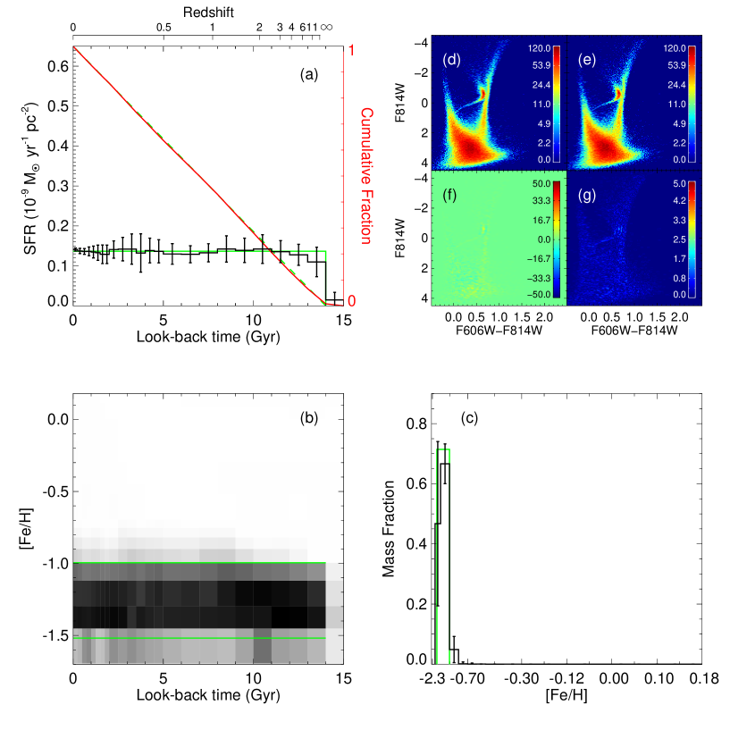
Figure 15: Mock galaxy with constant SFR, created and recovered with the BaSTI stellar evolution library. The green solid lines in panels (a) and (c) show the input SFH, while in panel (b) they delineate the upper and lower limits of the input metallicity range, between which the stars were uniformly distributed in each age bin. The green dashed line in panel (a) is the cumulative fraction of the input SFH.

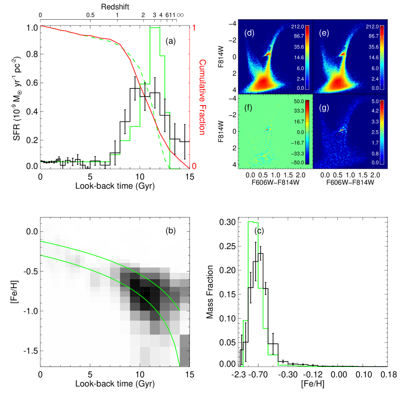
Figure 16: Same as Figure 15, but with a dSph-like SFH.

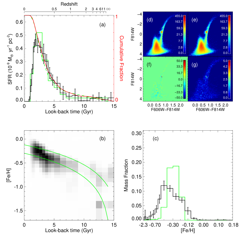
Figure 17: Same as Figure 15, but with a Leo A-like SFH.

References

- Agertz, Teyssier, & Moore (2011) Agertz O., Teyssier R., Moore B., 2011, MNRAS, 410, 1391
- Aparicio & Hidalgo (2009) Aparicio A., Hidalgo S. L., 2009, AJ, 138, 558
- Aparicio & Gallart (2004) Aparicio A., Gallart C., 2004, AJ, 128, 1465
- Barker et al. (2011) Barker M. K., Ferguson A. M. N., Cole A. A., Ibata R., Irwin M., Lewis G. F., Smecker-Hane T. A., Tanvir N. R., 2011, MNRAS, 410, 504
- Barker et al. (2007) Barker M. K., Sarajedini A., Geisler D., Harding P., Schommer R., 2007, AJ, 133, 1138
- Bernard et al. (2009) Bernard E. J., et al., 2009, ApJ, 699, 1742
- Bird, Kazantzidis, & Weinberg (2011) Bird J. C., Kazantzidis S., Weinberg D. H., 2011, MNRAS, submitted (astro-ph/1104.0933)
- Braun et al. (2009) Braun R., Thilker D. A., Walterbos R. A. M., Corbelli E., 2009, ApJ, 695, 937
- Brown et al. (2004) Brown T. M., Ferguson H. C., Smith E., Kimble R. A., Sweigart A. V., Renzini A., Rich R. M., 2004, AJ, 127, 2738
- Brown et al. (2006) Brown T. M., Smith E., Ferguson H. C., Rich R. M., Guhathakurta P., Renzini A., Sweigart A. V., Kimble R. A., 2006, ApJ, 652, 323
- Cole et al. (2007) Cole A. A., et al., 2007, ApJ, 659, L17
- Collins et al. (2011) Collins M. L. M., et al., 2011, MNRAS, 413, 1548
- Corbelli & Schneider (1997) Corbelli E., Schneider S. E., 1997, ApJ, 479, 244
- Courteau et al. (2011) Courteau S., Widrow L. M., McDonald M., Guhathakurta P., Gilbert K. M., Zhu Y., Beaton R. L., Majewski S. R., 2011, ApJ, 739, 20
- Cowie et al. (1996) Cowie L. L., Songaila A., Hu E. M., Cohen J. G., 1996, AJ, 112, 839
- Cuillandre et al. (2001) Cuillandre J.-C., Lequeux J., Allen R. J., Mellier Y., Bertin E., 2001, ApJ, 554, 190
- Dalcanton et al. (2009) Dalcanton J. J., et al., 2009, ApJS, 183, 67
- Di Matteo et al. (2008) Di Matteo P., Bournaud F., Martig M., Combes F., Melchior A.-L., Semelin B., 2008, A&A, 492, 31
- Duquennoy & Mayor (1991) Duquennoy A., Mayor M., 1991, A&A, 248, 485
- Fall & Efstathiou (1980) Fall S. M., Efstathiou G., 1980, MNRAS, 193, 189
- Fan, de Grijs, & Zhou (2010) Fan Z., de Grijs R., Zhou X., 2010, ApJ, 725, 200
- Fardal et al. (2007) Fardal M. A., Guhathakurta P., Babul A., McConnachie A. W., 2007, MNRAS, 380, 15
- Faria et al. (2007) Faria D., Johnson R. A., Ferguson A. M. N., Irwin M. J., Ibata R. A., Johnston K. V., Lewis G. F., Tanvir N. R., 2007, AJ, 133, 1275
- Ferguson et al. (2002) Ferguson A. M. N., Irwin M. J., Ibata R. A., Lewis G. F., Tanvir N. R., 2002, AJ, 124, 1452
- Ferguson et al. (2005) Ferguson A. M. N., Johnson R. A., Faria D. C., Irwin M. J., Ibata R. A., Johnston K. V., Lewis G. F., Tanvir N. R., 2005, ApJ, 622, L109
- Ferguson & Johnson (2001) Ferguson A. M. N., Johnson R. A., 2001, ApJ, 559, L13
- Gallart, Zoccali, & Aparicio (2005) Gallart C., Zoccali M., Aparicio A., 2005, ARA&A, 43, 387
- Gallazzi et al. (2008) Gallazzi A., Brinchmann J., Charlot S., White S. D. M., 2008, MNRAS, 383, 1439
- Galleti, Bellazzini, & Ferraro (2004) Galleti S., Bellazzini M., Ferraro F. R., 2004, A&A, 423, 925
- Girardi et al. (2000) Girardi L., Bressan A., Bertelli G., Chiosi C., 2000, A&AS, 141, 371
- Girardi & Salaris (2001) Girardi L., Salaris M., 2001, MNRAS, 323, 109
- Gogarten et al. (2010) Gogarten S. M., et al., 2010, ApJ, 712, 858
- Governato et al. (2009) Governato F., et al., 2009, MNRAS, 398, 312
- Grevesse & Noels (1993) Grevesse N., Noels A., 1993, in Origin and Evolution of the Elements, 15
- Guedes et al. (2011) Guedes J., Callegari S., Madau P., Mayer L., 2011, ApJ, 742, 76
- Hammer et al. (2010) Hammer F., Yang Y. B., Wang J. L., Puech M., Flores H., Fouquet S., 2010, ApJ, 725, 542
- Haywood (2008) Haywood M., 2008, MNRAS, 388, 1175
- Hidalgo et al. (2011) Hidalgo S. L., et al., 2011, ApJ, 730, 14
- Holland (1998) Holland S., 1998, AJ, 115, 1916
- Horne & Baliunas (1986) Horne J. H., Baliunas S. L., 1986, ApJ, 302, 757
- Ibata et al. (2001) Ibata R., Irwin M., Lewis G., Ferguson A. M. N., Tanvir N., 2001, Natur, 412, 49
- Ibata et al. (2005) Ibata R., Chapman S., Ferguson A. M. N., Lewis G., Irwin M., Tanvir N., 2005, ApJ, 634, 287
- Irwin et al. (2005) Irwin M. J., Ferguson A. M. N., Ibata R. A., Lewis G. F., Tanvir N. R., 2005, ApJ, 628, L105
- Jarosik et al. (2011) Jarosik N., et al., 2011, ApJS, 192, 14
- Kennicutt et al. (1987) Kennicutt R. C., Jr., Roettiger K. A., Keel W. C., van der Hulst J. M., Hummel E., 1987, AJ, 93, 1011
- Kroupa (2002) Kroupa P., 2002, Sci, 295, 82
- Layden et al. (1999) Layden A. C., Ritter L. A., Welch D. L., Webb T. M. A., 1999, AJ, 117, 1313
- Ma, Peng, & Gu (1997) Ma J., Peng Q.-H., Gu Q.-S., 1997, ApJ, 490, L51
- McConnachie et al. (2009) McConnachie A. W., et al., 2009, Natur, 461, 66
- McConnachie et al. (2010) McConnachie A. W., Ferguson A. M. N., Irwin M. J., Dubinski J., Widrow L. M., Dotter A., Ibata R., Lewis G. F., 2010, ApJ, 723, 1038
- Minchev et al. (2011) Minchev I., Famaey B., Combes F., Di Matteo P., Mouhcine M., Wozniak H., 2011, A&A, 527, A147
- Monelli et al. (2010) Monelli M., et al., 2010, ApJ, 720, 1225
- Muñoz-Mateos et al. (2011) Muñoz-Mateos J. C., Boissier S., Gil de Paz A., Zamorano J., Kennicutt R. C., Jr., Moustakas J., Prantzos N., Gallego J., 2011, ApJ, 731, 10
- Newton & Emerson (1977) Newton K., Emerson D. T., 1977, MNRAS, 181, 573
- Pietrinferni et al. (2004) Pietrinferni A., Cassisi S., Salaris M., Castelli F., 2004, ApJ, 612, 168
- Putman et al. (2009) Putman M. E., et al., 2009, ApJ, 703, 1486
- Quillen et al. (2009) Quillen A. C., Minchev I., Bland-Hawthorn J., Haywood M., 2009, MNRAS, 397, 1599
- Reid & Gizis (1997) Reid I. N., Gizis J. E., 1997, AJ, 113, 2246
- Reitzel, Guhathakurta, & Rich (2004) Reitzel D. B., Guhathakurta P., Rich R. M., 2004, AJ, 127, 2133
- Rich et al. (2004) Rich R. M., Reitzel D. B., Guhathakurta P., Gebhardt K., Ho L. C., 2004, AJ, 127, 2139
- Richardson (2010) Richardson J. C., 2010, PhD Thesis, University of Edinburgh
- Richardson et al. (2008) Richardson J. C., et al., 2008, AJ, 135, 1998
- Roškar et al. (2008a) Roškar R., Debattista V. P., Quinn T. R., Stinson G. S., Wadsley J., 2008a, ApJ, 684, L79
- Roškar et al. (2008b) Roškar R., Debattista V. P., Stinson G. S., Quinn T. R., Kaufmann T., Wadsley J., 2008b, ApJ, 675, L65
- Schlegel, Finkbeiner, & Davis (1998) Schlegel D. J., Finkbeiner D. P., Davis M., 1998, ApJ, 500, 525
- Schönrich & Binney (2009) Schönrich R., Binney J., 2009, MNRAS, 396, 203
- Sellwood & Binney (2002) Sellwood J. A., Binney J. J., 2002, MNRAS, 336, 785
- Sirianni et al. (2005) Sirianni M., et al., 2005, PASP, 117, 1049
- Skillman et al. (2003) Skillman E. D., Tolstoy E., Cole A. A., Dolphin A. E., Saha A., Gallagher J. S., Dohm-Palmer R. C., Mateo M., 2003, ApJ, 596, 253
- Sommer-Larsen, Götz, & Portinari (2003) Sommer-Larsen J., Götz M., Portinari L., 2003, ApJ, 596, 47
- Stetson (1994) Stetson P. B., 1994, PASP, 106, 250
- Stetson (1996) Stetson P. B., 1996, PASP, 108, 851
- Tabatabaei & Berkhuijsen (2010) Tabatabaei F. S., Berkhuijsen E. M., 2010, A&A, 517, A77
- Teyssier, Chapon, & Bournaud (2010) Teyssier R., Chapon D., Bournaud F., 2010, ApJ, 720, L149
- van der Wel et al. (2011) van der Wel A., et al., 2011, ApJ, 730, 38
- VandenBerg, Bergbusch, & Dowler (2006) VandenBerg D. A., Bergbusch P. A., Dowler P. D., 2006, ApJS, 162, 375
- Williams (2002) Williams B. F., 2002, MNRAS, 331, 293
- Williams et al. (2009a) Williams B. F., et al., 2009a, AJ, 137, 419
- Williams et al. (2009b) Williams B. F., Dalcanton J. J., Dolphin A. E., Holtzman J., Sarajedini A., 2009b, ApJ, 695, L15
- Williams et al. (2010) Williams B. F., et al., 2010, ApJ, 709, 135
- Wong et al. (2011) Wong K. C., et al., 2011, ApJ, 728, 119
- Wright et al. (1972) Wright M. C. H., Warner P. J., Baldwin J. E., 1972, MNRAS, 155, 337
- Wyse (2008) Wyse R. F. G., 2008, ASPC, 399, 445