Luminometer for the future International Linear Collider - simulation and beam test results

Abstract

LumiCal will be the luminosity calorimeter for the proposed International Large Detector of the International Linear Collider (ILC). The ILC physics program requires the integrated luminosity to be measured with a relative precision on the order of 10e-3, or 10e-4 when running in GigaZ mode. Luminosity will be determined by counting Bhabha scattering events coincident in the two calorimeter modules placed symmetrically on opposite sides of the interaction point. To meet these goals, the energy resolution of the calorimeter must be better than 1.5% at high energies. LumiCal has been designed as a 30-layer sampling calorimeter with tungsten as the passive material and silicon as the active material. Monte Carlo simulation using the Geant4 software framework has been used to identify design elements which adversely impact energy resolution and correct for them without loss of statistics. BeamCal, covering polar angles smaller than LumiCal, will serve for beam tuning, luminosity optimisation and high energy electron detection. Secondly, prototypes of the sensors and electronics for both detectors have been evaluated during beam tests, the results of which are also presented here.

1 Forward calorimetry at ILC

LumiCal is the proposed design for the luminosity calorimeter in the International Large Detector (ILD) [1] concept for the future International Linear Collider. It consists of two identical detectors placed symmetrically 2.5 m from the interaction point, and covers the angular range from 40 mrad to 69 mrad. BeamCal is proposed for the beam calorimeter, which will sit behind LumiCal at 3.45 m from the IP. BeamCal is described in detail in [2]. The locations of LumiCal and BeamCal in the ILD are shown in Figure 2.

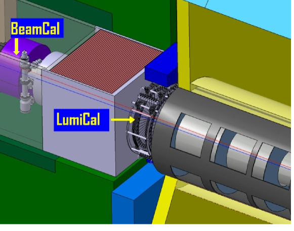
Figure 1: LumiCal and BeamCal in the ILC forward region.

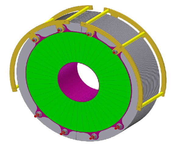
Figure 2: Mechanical model of LumiCal

2 LumiCal simulation

2.1 LumiCal description

The simulated model of LumiCal was built according to the reference design as described in [3]. A CAD drawing is shown in Figure 2. Each LumiCal module will consist of 30 layers of tungsten absorber with silicon sensors and electronics attached. There will also be space for mechanical support and cooling. The tungsten will extend radially from 76 mm for the inner edge to 280 mm for the outer (tentative). The sensitive radius will extend from 80 mm to 195.2 mm, with the rest of the space on the outside reserved for electronics and support. The sensor region is divided azimuthally into twelve equal tiles, each covering 30^o. Between each tile, there will be an uninstrumented 2.4 mm gap. Each tile is further divided azimuthally into four sectors, each covering 7.5^o, and radially into 64 pads with a 1.8 mm pitch. In order to fit around the beam pipe, the LumiCal modules will be built in two halves and then connected. A schematic of a half-plane of sensors is shown in Figure 4. The sensors are described in section 3.2. A prototype sensor tile is shown in Figure 4.

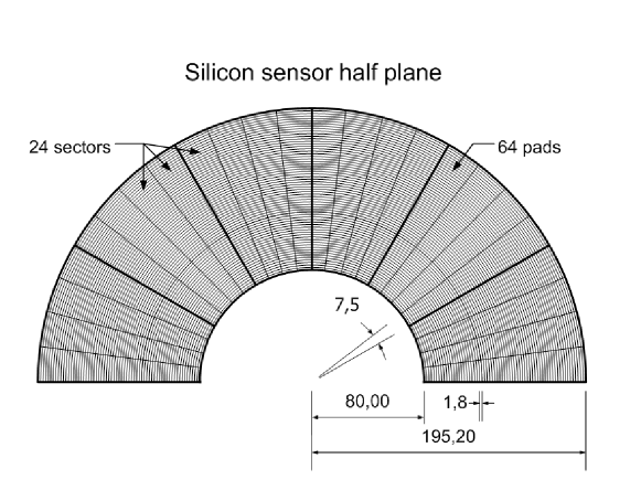
Figure 3: LumiCal sensor half-plane schematic.

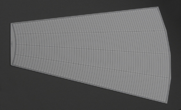
Figure 4: Photograph of LumiCal sensors.

2.2 Simulation parameters

The LumiCal simulation code, LuCaS, was built in Geant4 [4, 5], and the analysis of simulated events is performed using ROOT [6]. The geometric parameters are maintained to be identical to those in the collaborative ILC software framework [7], but LuCaS has the advantage of being more portable. This allowed it to be ported to the Cyfronet cluster computing facilities [8]. LumiCal has been studied extensively in simulation previously [9], but the energy resolution and energy scale uncertainty have only been studied with an idealized model with no gaps between sensor tiles (as described in section 2.1).

The simulations tested the response of LumiCal to single high-energy electrons between 5 GeV and 500 GeV, spread uniformly over the surface area of the detector. The simulation parameters are given in table 2.2.

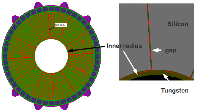
Figure 5: Simulated LumiCal model

Table 1: Simulation parameters

Parameter	Value
Particles	Single e-
Azimuthal range [rad]	$\phi\in[0,2\pi]$
Polar angle range [mrad]	$\theta\in[0.033,0.073]$
Energies [GeV]	5, 25, 50, 100, 150, 200,
	250, 500
Events/energy	5000
Physics lists	ILC Physics (LCPhysicsList)
Range cut	5 $\mu m$

Lastly, three versions of the LumiCal geometry were simulated: the reference design as described previously, and two variants. The first variant did not have alternate layers rotated by 3.75^o, so all the tile gaps were aligned directly. The purpose of this model was to make correction simpler at the expense of greater leakage in the gaps. The second variant was an idealized model of LumiCal with no dead areas in between tiles.

2.3 Tile gap effect

The tile gaps themselves cover approximately 3.5% of the total surface area of LumiCal. However, their influence extends further due to the Moliere radius of LumiCal, which is about 15 mm. Thus, 20% of showers may deposit some of their energy in the tile gaps, where it will not be recorded. This produces a long left tail of the raw total energy deposition per particle, as compared to ideal models of LumiCal (Figure 7). This is significant because it increases the RMS of the distribution of visible energy and makes reconstruction of the original energy more uncertain. It would be useful to have a method of correcting for the geometric irregularities that cause this effect, in order to reconstruct the energies of particles in the gaps as accurately as for particles in the sensors.

Previously, energy resolution was modeled using a single-parameter fit proportional to stochastic fluctuations in the shower, but a term can also be included to account for energy missed by the calorimeter:

$$\frac{\sigma_{E}}{E}=\sqrt{\frac{a^{2}}{E}+b^{2}},$$ (1)

where a is the stochastic parameter and b is the constant parameter. Further terms can be added to take into account other sources of noise, but were ignored since those sources were not included in the simulation.

The energy resolution for particles of a given energy is calculated from simulation by dividing the RMS of the reconstructed energy by the initial energy. This is performed for different energies (here, eight) and the results are compared with equation 1.

2.4 Correcting for the tile gaps

Cuts

Two methods were investigated for ameliorating the effect of the tile gaps. The first was simply to discount the energy deposition from primary electrons incident on the tile gaps. The cut was defined as a distance from the center of each gap - that is, the energy deposition from all particles incident within a certain distance from the gaps were ignored. For example, Figure 7 shows the energy deposited by electrons plotted against the azimuthal angle of the initial point of impact, with a 4.8 mm selection cut (measured from the center of the tile gap). Only the particles labeled as “sensor hits” – primary particles which hit the sensors at least the cut width away from a tile gap – were considered in the calculation of energy resolution. In Figure 7, sensor hits are shown as blue squares and gap hits are shown as red circles.

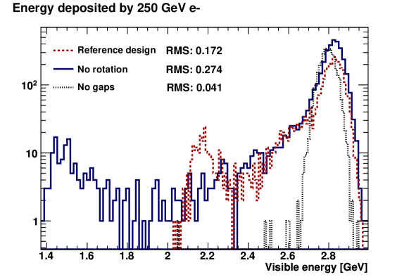
Figure 6: Visible energy at 250 GeV, showing the largest tail for the unrotated geometry and no tail for the gapless, ideal geometry. The y-axis is shown in log scale to emphasize the tails.

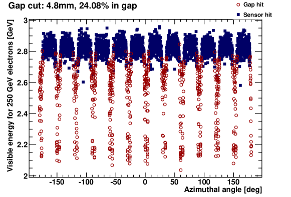
Figure 7: Energy deposition in the tile gaps (gap hits shown in red).

Fits

The CALICE collaboration showed that for the ILD ECAL, the energy deposition in similar-style gaps could be fit with a Gaussian distribution [10]. Applying similar methods to the LumiCal simulation data, it was found that the gaps could be fit with a Lorentz distribution and a Gaussian distribution, allowing for the energy lost in the gaps to be corrected. The Lorentz distribution fits the sides, and the Gaussian distribution fits the peak. The equation used for fitting is given in equation 2:

$$\mathit{E}(x)=A-\frac{B}{(1+(\frac{x-C}{D})^{2})}-E\cdot e^{-F\cdot x^{2}}$$ (2)

Energy deposition was fit against the Cartesian distance of the hit from the nearest tile gap, instead of azimuthal angle. A fitted plot is shown in Figure 8. The unrotated geometry variant was used for this analysis as a proof-of-principle. This geometry is nevertheless attractive from an engineering standpoint because it would reduce the complexity of construction of the calorimeter.

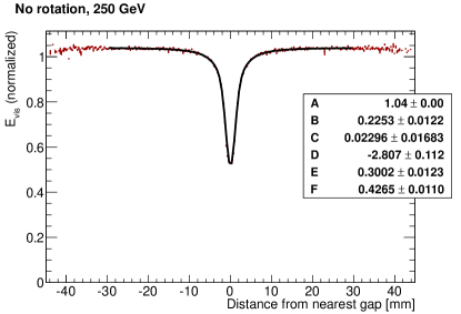
Figure 8: 250 GeV energy deposition for all $\phi$ folded onto one tile width and normalized to the average deposition in the center of each tile.

Figure 10 shows a comparison of the energy resolution performance of the LumiCal variants. The geometry of LumiCal was slightly modified for better comparison with the fitting method - there was no rotation between subsequent layers of LumiCal. The worst performance came from the case without any correction. The smallest cut, excluding only particles that hit directly in the tile gaps, already improves the energy resolution by a factor of 2. The ideal LumiCal geometry (no gaps) gives the best energy resolution, as expected. The fitting method approaches the same performance as the ideal LumiCal design, and is nearly identical to a 10 mm cut (or $\sim$40% of particles cut). A comparison of fit parameters is shown in Figure 10. The uncertainties on the stochastic parameters calculated from the cutting methods are much larger than those from the $\phi$-fitting and cases. Furthermore, the constant parameter for $\phi$-fitting almost completely compensates for leakage, compared to the no-gaps case. This suggests that performing the $\phi$-fitting correction is the best way to proceed in making the energy resolution of LumiCal geometrically uniform.

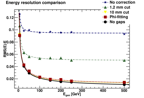
Figure 9: Comparison of different cut widths (width on each side of the gap) with fit-corrected case and ideal gap-less calorimeter case. Error bars are too small to be seen at this scale.

Figure 10: Comparison of fit parameters for different methods of determining energy resolution. The stochastic parameter is given on the left, and the constant parameter is given on the right.

3 Beam test

The main purpose of the beam test was to test the performance of the readout chain from the solid-state sensors (Si or GaAs) up to the front-end ASICs, which were all custom designed by the FCAL collaboration. The beam test was performed at DESY-Hamburg. A description of the facilities can be found at [11].

3.1 Beam area setup

Beamline 22 at DESY contains the ZEUS MVD telescope described in [12]. The telescope, shown schematically in Figure 12, consists of three planes of sensors placed along the beam axis. Each plane is comprised of two mutually perpendicular sets of Si microstrips with a 320 $\mu$m pitch. Using the combined data for the three planes, the track of an electron from the beam line can be determined and the point of impact on the device under test (DUT) accurately calculated.

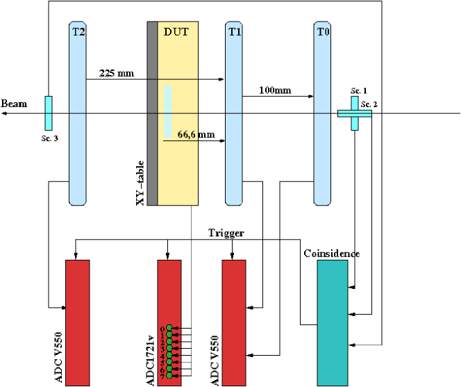
Figure 11: Schematic showing telescope planes and trigger electronics, with the DUT in between telescope planes 1 and 2 (indexed from 0).

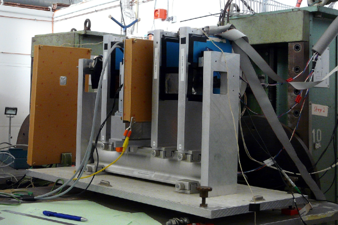
Figure 12: Photograph of BeamCal sensors in place and LumiCal sensors behind telescope

Figure 12 is a photograph of the setup used for the BeamCal data runs. The tan DUT box in between planes 1 and 2 contains the BeamCal readout chain. The tan box after the telescope contains the LumiCal readout chain, and was placed there for preliminary testing purposes. The BeamCal box was mounted on a two-dimensional motorized translation stage so that different parts of the sensor could be irradiated. The LumiCal box was later moved to the DUT position.

3.2 Readout chain

Figure 13(a) shows a photograph of the readout chain with the LumiCal sensors shown in Figure 4. The BeamCal readout chain was identical except for the type of sensors (see section 3.4). The fanouts were glued to the sensors and connected to the custom-designed front end ASICs [13]. The readout chain also consisted of output buffers, biasing and power blocks, and a commercial ADC (14-bit, 8-channel Caen VME-1724 for LumiCal; for BeamCal as in Figure 12). In total, sixteen sensor pads were connected to the FE ASICs - eight from the bottom of the sensor and eight from the top. This encompassed the widest range of sensor sizes and fanout lengths, for crosstalk measurements. For LumiCal, the sensors consisted of one tile produced by Hamamatsu, with geometry as described in section 2.1. The tile was made from 320 $\mu$m-thick n-doped Si bulk with p+ pads and Al metallization [14].

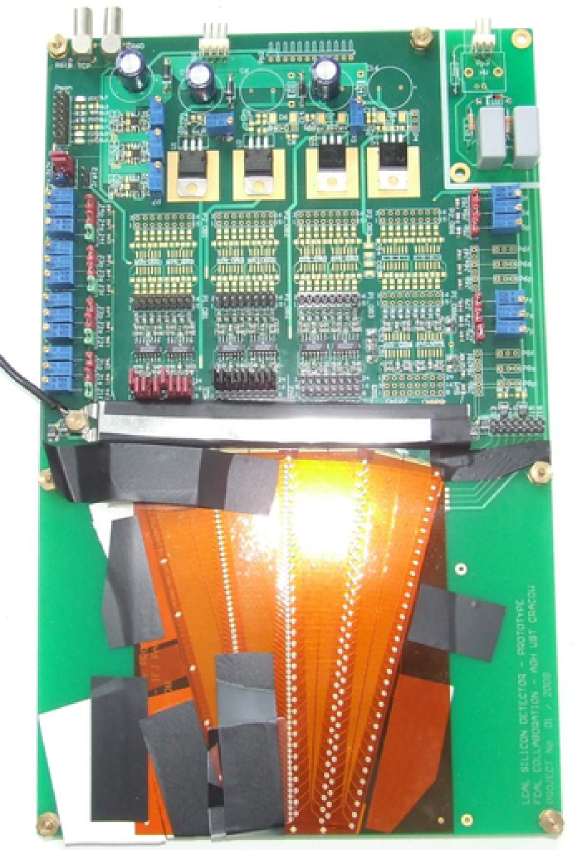
(a) Complete readout chain: 16 connected sensor pads with fanout, FE ASICs bonded to PCB, output buffers, and biasing and power blocks.

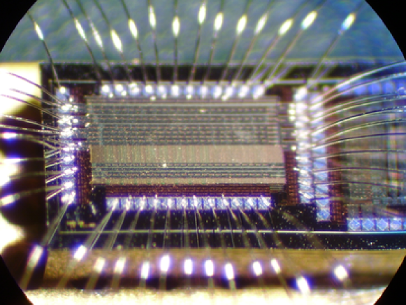
(b) Picture of the custom FE-ASIC

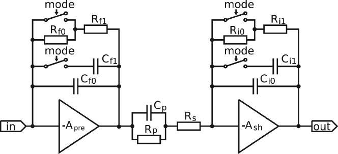
(c) FE ASIC schematic. “Mode” switch allows the feedback path to be chosen. This schematic shows resistive feedback, but an active feedback version was also used.

Figure 13: Hardware and electronics under test.

Aside from the GaAs BeamCal sensors (described later), the two eight-channel front-end ASICs were the most important element of the readout chain being tested. A picture of the ASIC is shown in Figure 13(b), and a block diagram is shown in Figure 13(c).

The FE ASICs feature a mode switch that allows the ASICs to operate in one of two modes: “calibration” mode and “physics” mode. The schematic in Figure 13(c) shows the mode switch with passive (resistive) feedback. For each ASIC, half channels used this type of feedback while the other half used active feedback. The ASIC design is described in detail in [13], and an analysis of the performance can be found in [15].

3.3 LumiCal results

Preliminary LumiCal beamtest results have been previously reported in an internal FCAL memo [15]. Figure 15 (top) shows the time response of a single front-end channel to different amounts of energy deposition. As expected, the shape of the signal is independent of the signal amplitude. Figure 15 (bottom) shows the energy deposition spectrum in a single channel for 4.5 GeV electrons from the DESY beamline. The spectrum for all pads is well fit by a Landau distribution. The set of spectra were used to find the gain of the channels. The spread of the gain within each channel type is within 1%. Signal-to-noise ratio, even for the largest sensor capacitances, is about 18.

In multi-channel designs, it is important to ensure good channel-to-channel separation. Figure 15 shows the response of eight channels under test to a particle passing through a sensor pad in the center of the instrumented area. In channel four, a signal corresponding to approximately 10 MIPS was measured. The lower part of Figure 15 shows a magnified image of the nearest-neighbor baseline signals. The amount of crosstalk was less than 1%.

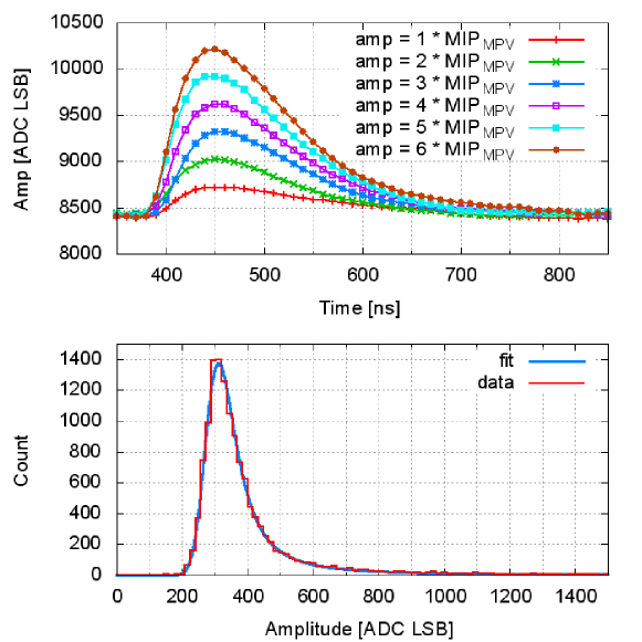
Figure 14: Top: Response over time to electrons of different energies was uniform. Bottom: Spectrum of signals shows a Landau distribution.

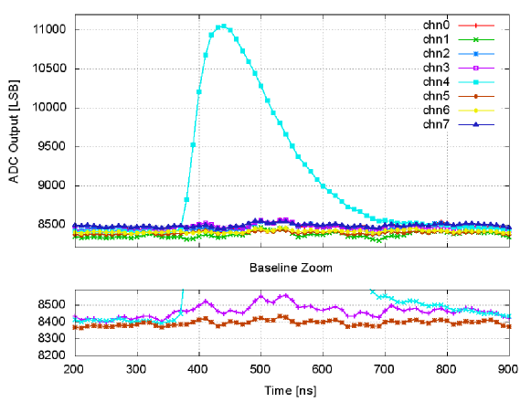
Figure 15: Bottom shows neighboring signals $<$ 1%

3.4 BeamCal results

The BeamCal sensors, shown in Figure 16, have different segmentation from the LumiCal sensors shown in Figure 4. The square pad size was choosen to be half of the Moliere radius of electromagnetic showers for high-energy electrons. Additionally, because BeamCal will operate in a radiation-high environment, the sensors are proposed to be made of GaAs as a radiation hard material candidate. GaAs samples were tested in electron beam up to 1.5 MGy [16]. The beam test for BeamCal was intended in part to test the qualities of GaAs for high-energy physics calorimetry.

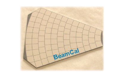
Figure 16: Photograph of GaAs sensor prototype

One important test of the BeamCal sensors was to check for signal uniformity across each pad. Figure 18 shows a single 5mm x 5mm pad in red divided into four regions, indicated by the four squares outlined in blue. In Figure 18, it can be seen that all four regions of the pad generated identical signal spectra, and furthermore which were all shaped like a Landau distribution, as expected. The particle detection efficiency was $\sim$100%, and SNR was $\sim$20.

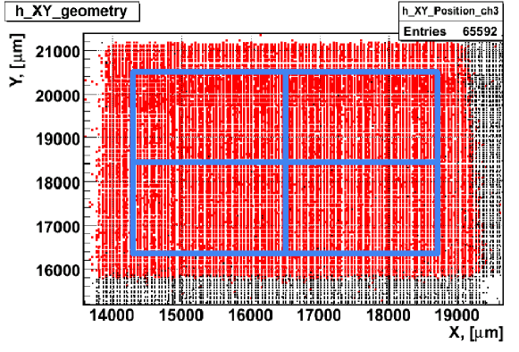
Figure 17: Pad regions in BeamCal.

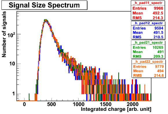
Figure 18: Signals from the four pad areas identified in blue

The BeamCal beam test results can be found in greater detail in [17].

4 Conclusions

The gap-fitting method provides a promising way to recover missing energy during calculation of energy resolution. This can be done both in the reference LumiCal geometry and in the unrotated LumiCal geometry, in which case the performance of the fitting is slightly better. However, should an unrotated LumiCal be a viable option, further studies must be done to examine the effect of aligned tile gaps on detector hermeticity.

The beam test proved to be a successful test of the front-end electronics readout chain developed for both LumiCal and BeamCal. The novel FE ASIC demonstrated uniform time response to signals of different amplitudes, good SNR, and had crosstalk of less than 1% between neighboring channels. BeamCal GaAs sensors showed good charge uniformity across the sensor pads, supporting their cause as candidates for solid-state sensors in radiation-hard environments.

5 Acknowledgments

This work was supported by the Commission of the European Communities under the 7^th Framework Programme “Marie Curie ITN”, grant agreement number 214560. It was also supported in part by the Polish Ministry of Science and Higher Education under contract nr 1246/7.PR UE/2010/7. The authors would also like to thank Cyfronet in Krakow for computing resources, and Ingrid-Maria Gregor and Artem Kravchenko for their work at the DESY test beam facility.

References

- [1] More information about ILD can be found at http://www.ilcild.org/.
- [2] BeamCal parameters are available on the web at http://fcal.desy.de/e107470/e107471/.
- [3] W. Daniluk, E. Kielar, J. Kotula, A. Moscczynski, K. Oliwa, B. Pawlik, W. Wierba, L. Zawiejski, J. Aguilar, Redesign of LumiCal mechanical structure, Eudet-Memo-2010-06Available at http://www.eudet.org/e26/e28/.
- [4] S.Agostinelli, et al., Geant 4 - a simulation toolkit, NIM-A 503 (1) (2003) 250–303.
- [5] J.Allison, et al., Geant4 developments and applications, IEEE Transactions on Nuclear Science 53 (1) (2006) 270–278.
- [6] R. Brun, F. Rademakers, Root - an object oriented data analysis framework, AIHENP’96 Workshop, 1996.
- [7] http://ilcsoft.desy.de/portal.
- [8] http://www.cyfronet.pl/en/.
- [9] I. Sadeh, Luminosity measurement at the International Linear Collider, Master’s thesis, Tel Aviv University (2009).
- [10] C. Adloff, et al., Response of the calice si-w electromagnetic calorimeter physics prototype to electrons, NIM-A 608 (2009) 372–383.
- [11] http://adweb.desy.de/testbeam/.
- [12] See http://www.desy.de/gregor/short_intro.html for information and sources about the MVD telescope.
- [13] M. Idzik, S. Kulis, D. Przyborowski, Development of front-end ASICs for the luminosity detector at ILC, NIM-A.
- [14] J. Blocki, W. Daniluk, E. Kielar, J. Kotula, A. Moszczynski, K. Oliwa, B. Pawlik, W. Wierba, L. Zawiejski, J. Aguilar, Silicon sensors prototype for lumical calorimeter, Eudet-Memo-2009-07Available at http://www.eudet.org/e26/e28/.
- [15] S.Kulis, J. Aguilar, M. Chrzaszcz, W. Wierba, L. Zawiejski, E. Kielar, O. Novgorodova, H. Henschel, W. Lohmann, S. Schuwalow, K. Afanaciev, A. Ignatenko, I. Levy, M. Idzik, K. J, A. Moszczynski, K. Oliwa, B. Pawlik, W. Daniluk, Test beam studies of the LumiCal prototype, Eudet-memo-2010-09Available at http://www.eudet.org/e26/e28/.
- [16] H. Abramowicz, et al., Forward instrumentation for ilc detectors, Journal of Instrumentation 5 (P12002).
- [17] O. Novgorodova, Forward calorimeters for the future electron-positron linear collider detectors, in: The XIXth International Workshop on High Energy Physics and Quantum Field THeory, 2010, poS(QFTHEP2010)030.