Asymptotics of Selberg-like integrals by lattice path counting

Abstract

We obtain explicit expressions for positive integer moments of the probability density of eigenvalues of the Jacobi and Laguerre random matrix ensembles, in the asymptotic regime of large dimension. These densities are closely related to the Selberg and Selberg-like multidimensional integrals. Our method of solution is combinatorial: it consists in the enumeration of certain classes of lattice paths associated to the solution of recurrence relations.

1 Introduction

Let $N$ be a positive integer and $\mathcal{C}=[0,1]^{N}$ be an $N$-dimensional hypercube. The integral

$$S(\alpha,\gamma,\beta)=\int_{\mathcal{C}}|\Delta(T)|^{\beta}\prod_{i=1}^{N}T_{i}^{\alpha-1}(1-T_{i})^{\gamma-1}dT_{i},$$ (1)

where $\Delta(T)=\prod_{1\leq i<j\leq N}(T_{i}-T_{j})$ is the Vandermonde determinant, was evaluated by Selberg. It has found applications in many different areas of mathematics [1, 2, 3] and physics [4, 5, 6], in particular in the theory of random matrices [7, 8]. A recent review of applications as well as of the history of the field can be found in [9]. Within the context of random matrix theory the constant $\beta$ identifies the orthogonal, unitary and symplectic universality classes and takes value in the set $\{1,2,4\}$. The normalized function

$$P^{\alpha,\gamma}_{\beta}(T)=\frac{1}{S(\alpha,\gamma,\beta)}|\Delta(T)|^{\beta}\prod_{i=1}^{N}T_{i}^{\alpha-1}(1-T_{i})^{\gamma-1}$$ (2)

is the joint probability density of the eigenvalues of matrices from the Jacobi $\beta$-Ensemble [8]. The average value of any function of the eigenvalues $f(T)$ is given by the multiple integral

$$\langle f(T)\rangle=\int_{\mathcal{C}}f(T)P^{\alpha,\gamma}_{\beta}(T)d^{N}T,$$ (3)

with $d^{N}T=\prod_{i}dT_{i}$.

One particular application involves quantum electronic transport in mesoscopic structures [5]. If there are $N_{1}$ incoming channels and $N_{2}$ outgoing channels, the system may be described by a $N_{2}\times N_{1}$ transmission matrix $t$ whose element $t_{ij}$ is the probability amplitude of transmission from channel $j$ to channel $i$. For systems with chaotic classical dynamics the random matrix approach to the problem consists in assuming the system’s unitary $S$-matrix to be a random element of a circular $\beta$-ensemble. This is equivalent to assuming the hermitian matrix $\mathcal{T}=tt^{\dagger}$ to be uniformly distributed in the Jacobi $\beta$-Ensemble [10] with $N={\rm min}\{N_{1},N_{2}\}$, $\alpha=\frac{\beta}{2}(|N_{2}-N_{1}|+1)$ and $\gamma=1$.

In the above context (with $\gamma=1$) the average value of quantities like

$${\rm Tr}[\mathcal{T}^{n}]=\sum_{i=1}^{N}T_{i}^{n}$$ (4)

can be used to characterize universal statistical properties of quantum chaotic transport. Exact results appeared for small $n$ in [11, 12, 13, 14] and for general $n$ in [15, 16]. In this last work the present author used a result of Kaneko [2] and Kadell [17] which gives the average value of any Schur function of the eigenvalues, an approach that was later taken further in [18, 19]. For large numbers of channels, a generating function for the average value of (4) was presented in [20], and an explicit expression appeared in [13].

We are concerned with the asymptotic regime $N\gg 1$ of the average value of (4) with respect to the probability density (2). Special cases of this problem were recently discussed in [21], by using the method from [16] and taking $N\gg 1$ in the last step. It was then noticed that the results had combinatorial interpretations, but no reason for that was provided. The authors of [21] also conjectured that in this regime the average has a factorization property, i.e. $\langle f(T)g(T)\rangle$ becomes asymptotically equal to the product $\langle f(T)\rangle\langle g(T)\rangle$ if the functions $f(T)$ and $g(T)$ depend on disjoint sets of variables. If this is true, then the quantity $\langle T_{1}^{n}\rangle$ becomes indeed the most interesting one to compute.

We also consider the asymptotic regime $N\gg 1$ of the average value of (4) within the Laguerre ensemble of random matrices. It that case the eigenvalues belong to $[0,\infty)$ and have a joint probability density given by

$$L^{\alpha,\epsilon}_{\beta}(T)=\frac{1}{Y(\alpha,\beta,\epsilon)}|\Delta(T)|^{\beta}\prod_{i=1}^{N}T_{i}^{\alpha}e^{-\epsilon T_{i}},$$ (5)

where $Y(\alpha,\beta,\epsilon)$ is a known normalization constant which is given by a Selberg-like integral. This also finds an application in the area of quantum chaotic transport [22, 23]. The eigenvalues of the Wigner-Smith time-delay matrix $Q=-i\hbar S^{-1}\partial S/\partial E$ (where $E$ is the energy) are called proper delay times, $T_{i}$. The inverse delay times $1/T_{i}$ are distributed according to the Laguerre ensemble with $\alpha=\beta N/2$ and $\epsilon=-\beta N/(2\gamma)$ where $\gamma$ is the classical decay rate of the system.

2 Statement of results

We obtain an explicit formula for $\langle T_{1}^{n}\rangle$, in the asymptotic regime, valid for arbitrary values of $\beta$ (not restricted to the set $\{1,2,4\}$) and for arbitrary parameters $\alpha$ and $\gamma$, which are allowed to grow linearly with $N$ as is sometimes required. Let $[x]$ denote the integer part of $x$ and let

$$C_{n}={2n\choose n}\frac{1}{n+1}$$ (6)

be the Catalan numbers. We show that, asymptotically,

$$\langle T_{1}^{n}\rangle=A_{2}\sum_{m=0}^{n-1}{n-1\choose m}(-1)^{m}A_{3}^{n-1-m}\sum_{k=0}^{\left[\frac{m+1}{2}\right]}{m-k\choose k}C_{m-k}(A_{1}A_{2})^{m-k}(1-A_{3})^{k},$$ (7)

where

$$A_{1}=\frac{\beta N}{2(\alpha+\gamma+\beta N)},\quad A_{2}=\frac{2\alpha+\beta N}{2(\alpha+\gamma+\beta N)},\quad A_{3}=A_{1}+A_{2}.$$ (8)

The above formula generalizes all special cases that have so far been considered. Our derivation is essentially combinatorial, and consists of finding a recurrence relation and then turning its solution into the problem of enumerating certain lattice paths. In the course of the calculation we prove the factorization conjecture already mentioned, for polynomial functions $f(T)$ and $g(T)$.

For the Laguerre $\beta$-Ensemble (5) we show that the factorization conjecture holds as well and that the relevant asymptotic average value is given by

$$\langle T_{1}^{n}\rangle=A_{2}\sum_{m=0}^{\left[\frac{n-1}{2}\right]}{n-1\choose 2m}C_{m}(A_{1}A_{2})^{m}A_{3}^{n-1-2m}$$ (9)

where

$$A_{1}=\frac{\beta N}{2},\quad A_{2}=\alpha+A_{1},\quad A_{3}=A_{1}+A_{2}.$$ (10)

We also consider the analogous problem for the distribution of proper delay times. It was shown in [24], by other means, that the solution contains the Schröder numbers; we present a combinatorial proof of that.

We note that the Laguerre and Jacobi ensembles are also widely studied in the context of multivariate statistical analysis [8, 25], where they are known as the Wishart distribution and the multivariate beta distribution. Moments of the latter were considered in [26].

The paper is organized as follows. In Section 3 we consider the quantum transport case, which involves Jacobi Ensembles with $\gamma=1$. This is the simplest version of the problem. The lattice paths involved are Dyck paths, which have only two types of steps. In Section 4 we turn to the Laguerre Ensembles, which are second in the complexity scale. The lattice paths involved are now Motzkin paths, which have three types of steps. In Section 5 we consider the distribution of proper delay times in quantum chaotic scattering (closely related to Laguerre). The lattice paths that appear in that case are Schröder paths. Finally, in Section 6 we come to Jacobi Ensembles with arbitrary $\gamma$, which involve lattice paths with four types of steps.

3 Jacobi Ensembles with $\gamma=1$

Let $f(T)=\prod_{i=1}^{m-1}T_{i}^{\lambda_{i}}$. We will show that $\langle f(T)T_{m}^{n}\rangle\approx\langle f(T)\rangle\langle T_{m}^{n}\rangle$ in the asymptotic regime $N\gg 1$. To that end let us define $Q=f(T)T_{m}^{n+1}P^{\alpha}_{\beta}(T)$, with $n>\lambda_{i}$. Taking into account that

$$\frac{dP^{\alpha}_{\beta}}{dT_{m}}=\frac{(\alpha-1)}{T_{m}}P^{\alpha}_{\beta}(T)+\beta P^{\alpha}_{\beta}(T)\sum_{i\neq m}\frac{1}{T_{m}-T_{i}}$$ (11)

we can write the derivative of $Q$ with respect to $T_{m}$,

$$\frac{dQ}{dT_{m}}=f(T)P^{\alpha}_{\beta}(T)\left[(n+\alpha)T_{m}^{n}+\beta\sum_{i\neq m}\frac{T_{m}^{n+1}}{T_{m}-T_{i}}\right].$$ (12)

Notice that

$$\delta Q=\int_{0}^{1}dT_{m}\frac{dQ}{dT_{m}}$$ (13)

does not depend on the value of $n$. We will use this fact to find a recurrence relation. This idea goes back to Aomoto [27].

The integral of (12) is

$$\int_{\mathcal{C}}\frac{dQ}{dT_{m}}d^{N}T=(n+\alpha)\langle f(T)T_{m}^{n}\rangle+\beta\sum_{i\neq m}\left\langle\frac{f(T)T_{m}^{n+1}}{T_{m}-T_{i}}\right\rangle.$$ (14)

But

$$\sum_{i\neq m}\left\langle\frac{f(T)T_{m}^{n+1}}{T_{m}-T_{i}}\right\rangle=\sum_{i<m}\left\langle\frac{f(T)T_{m}^{n+1}}{T_{m}-T_{i}}\right\rangle+(N-m)\left\langle\frac{f(T)T_{m}^{n+1}}{T_{m}-T_{m+1}}\right\rangle.$$ (15)

By symmetry,

$$\left\langle\frac{f(T)T_{m}^{n+1}}{T_{m}-T_{m+1}}\right\rangle =\frac{1}{2}\left\langle f(T)\frac{T_{m}^{n+1}-T_{m+1}^{n+1}}{T_{m}-T_{m+1}}\right\rangle$$ (16)

$$=\frac{1}{2}\sum_{a=0}^{n}\big{\langle}f(T)T_{m}^{n-a}T_{m+1}^{a}\big{\rangle}.$$ (17)

Also, in the same vein

$$\left\langle\frac{f(T)T_{m}^{n+1}}{T_{m}-T_{i}}\right\rangle=\frac{1}{2}\sum_{a=0}^{n-\lambda_{i}}\big{\langle}f(T)T_{i}^{a}T_{m}^{n-a}\big{\rangle}.$$ (18)

Every term in (15) is of the same order in the limit $N\to\infty$, and we can thus make the approximation

$$\sum_{i\neq m}\left\langle\frac{f(T)T_{m}^{n+1}}{T_{m}-T_{i}}\right\rangle=N\left\langle\frac{f(T)T_{m}^{n+1}}{T_{m}-T_{m+1}}\right\rangle+O(1).$$ (19)

This is the crucial step towards the factorization property, because we have just ignored the terms of the sum containing the variables that appear in $f(T)$. They are the ones that obstruct the factorization for finite $N$.

From now on we simply ignore the error terms and keep in mind that the limit $N\to\infty$ is implicit. Defining the function

$$D^{i,j}_{n}=\sum_{a=1}^{n-1}T_{i}^{n-a}T_{j}^{a}$$ (20)

we have

$$\int_{\mathcal{C}}\frac{dQ}{dT_{m}}d^{N}T=\left[\alpha+\beta N\left(1-\frac{\delta_{n,0}}{2}\right)\right]\langle f(T)T_{m}^{n}\rangle+\frac{\beta N}{2}\langle f(T)D^{m,m+1}_{n}\rangle,$$ (21)

where we have neglected $n$ against $\alpha+\beta N$ (remember that $\alpha$ may grow with $N$).

We have seen that the above does not depend on the value of $n$. In particular, for $n=0$ it gives $(\alpha+\beta N/2)\langle f(T)\rangle$ and for $n=1$ it gives $(\alpha+\beta N)\langle f(T)T_{m}\rangle.$ Comparing the formulas for general $n$ and $n=0$ we obtain

$$\langle f(T)T_{m}^{n}\rangle=A_{2}\langle f(T)\rangle-A_{1}\langle f(T)D_{n}^{m,m+1}\rangle,$$ (22)

where

$$A_{1}=\frac{\beta N}{2(\alpha+\beta N)},\quad A_{2}=\frac{2\alpha+\beta N}{2(\alpha+\beta N)}.$$ (23)

Recurrence relation (22) proves the factorization conjecture, at least for polynomials. This is because the function $f(T)$ does not change when the relation is iterated, so it should be clear that it results in $\langle f(T)T_{m}^{n}\rangle=\langle f(T)\rangle\langle T_{m}^{n}\rangle$.

The use of letters $A_{1},A_{2}$ comes from the quantum transport setting, where if $N\gg 1$ we obtain $A_{i}\approx N_{i}/(N_{1}+N_{2})$. Also, in that case $\alpha$ is proportional to $\beta$, causing the final result to be independent of $\beta$. Notice that if $\alpha$ is held fixed in the limit of large $N$ we end up with $A_{1}=A_{2}=1/2$.

We now turn to our main objective, which is the calculation of the basic quantity $\langle T^{n}\rangle$. We omit the index of the variable since it is irrelevant. Let us define

$$\mathcal{D}_{n}=\sum_{a=1}^{n-1}\langle T^{n-a}\rangle\langle T^{a}\rangle.$$ (24)

We have $\langle T^{0}\rangle=1$, $\langle T^{1}\rangle=A_{2}$ and the recurrence relation

$$\langle T^{n}\rangle=A_{2}-A_{1}\mathcal{D}_{n},\quad n\geq 2.$$ (25)

We may write this as

$$\langle T^{n}\rangle=A_{2}-A_{1}M_{n}+2A_{1}\langle T^{n}\rangle,\quad n\geq 1,$$ (26)

where we have defined

$$M_{n}=\sum_{a=0}^{n}\langle T^{n-a}\rangle\langle T^{a}\rangle.$$ (27)

It is possible to obtain the ordinary generating function

$$F(x)=1+\sum_{n\geq 1}\langle T^{n}\rangle x^{n}.$$ (28)

Since

$$[F(x)]^{2}=1+\sum_{n\geq 1}M_{n}x^{n}$$ (29)

we get the algebraic relation

$$F=1+\frac{A_{2}x}{1-x}+2A_{1}(F-1)-A_{1}(F^{2}-1),$$ (30)

which can be solved to give

$$F(x)=1-\frac{1}{2A_{1}}+\frac{1}{2A_{1}}\sqrt{1+\frac{4A_{1}A_{2}x}{1-x}}.$$ (31)

The generating function of course provides $\langle T^{n}\rangle$ for any value of $n$. However, an explicit formula for this quantity can be obtained by representing the recurrence relation pictorially and turning its solution into a lattice path counting problem.

Let us start with a brief example. The recurrence relation (25) gives

$$\langle T_{1}^{4}\rangle=A_{2}-A_{1}(\langle T_{1}^{3}T_{2}\rangle+\langle T_{1}^{2}T_{2}^{2}\rangle+\langle T_{1}T_{2}^{3}\rangle).$$ (32)

The coefficient of $A_{1}$ contains all ordered partitions of $4$ into two parts. In the next step we have

$$A_{2}-A_{1}\Big{[}A_{2}(\langle T_{1}\rangle+\langle T_{1}^{2}\rangle+\langle T_{1}^{3}\rangle)-A_{1}(\langle T_{1}T_{2}T_{3}^{2}\rangle+\langle T_{1}T_{2}^{2}T_{3}\rangle+\langle T_{1}^{2}T_{2}T_{3}\rangle)\Big{]}.$$ (33)

Now the coefficient of $A_{1}^{2}$ has the ordered partitions of $4$ into three parts. The coefficient of $A_{1}A_{2}$ has the ordered partitions –into one part– of the numbers up to three. At every step, when the power of $A_{1}$ is increased the number of parts in the ordered partitions also increases; on the other hand, when the power of $A_{2}$ increases one part of the previous partitions is removed.

Let $[N,m]$ denote the set of all ordered partitions of $N$ into $m$ parts. We can represent a general step in the iteration of the recurrence relation as

$$[ N,m]\xrightarrow{A_{1}}[N,m+1]$$

$$\downarrow A_{2}\hskip 51.21504pt\downarrow A_{2}$$

$$\bigcup_{n=1}^{N-1}[n, m-1]\xrightarrow{A_{1}}\bigcup_{n=1}^{N-1}[n,m]$$

Notice the commutativity of the diagram. We may therefore think of $A_{1}$ and $A_{2}$ as directions in which we can move as we proceed with the calculation. If we further simplify notation by writing $(N,m)=\bigcup_{n=1}^{N}[n,m]$ then Figure 1 codifies the recurrence relation.

Figure 1: The recurrence relation (25) may be mapped into a path-counting problem if we associate with $A_{1}$ and $A_{2}$ different directions of movement. In the $A_{1}$ direction we increase the number of parts of the ordered partitions, while in the $A_{2}$ direction we eliminate one part. If a path hits the lowest horizontal line it stops. The number of terms is constant along falling steps.

We start at $[n,1]$, which just represents $\langle T_{1}^{n}\rangle$. Iteration of the recurrence relation then produces all possible sequences of rising and falling steps that remain above the $(\cdot,1)$ horizontal line. A path ends if and only if it drops below that line. The final result for $\langle T^{n}\rangle$ will therefore be equal to $A_{2}$ times a polynomial in $(-A_{1}A_{2})$ of degree $n-1$. The coefficient of $(-A_{1}A_{2})^{p}$ contains two contributions. First, the number of terms in the set $[n,p+1]$ (because moving in the $A_{2}$ direction does not change the number of terms). This is the number of ordered partitions of $n$ into $p+1$ parts and is given by $\binom{n-1}{p}$. Second, the number of different paths leading from $[n,1]$ to $(n-p,1)$. Clearly, the relevant paths are Dyck paths: lattice paths with steps $(1,1)$ and $(1,-1)$ that never fall below the $x$ axis. The number of such paths containing $2p$ steps is well known to be the Catalan number, $C_{p}$. In conclusion,

$$\langle T^{n}\rangle=A_{2}\sum_{p=0}^{n-1}\binom{n-1}{p}(-1)^{p}C_{p}(A_{1}A_{2})^{p}.$$ (34)

This calculation has been sketched previously in [13].

4 Laguerre Ensembles

Before tackling the general Jacobi ensembles, we first consider the Laguerre case. We now have the kernel

$$L^{\alpha,\epsilon}_{\beta}(T)=\frac{1}{Y}|\Delta|^{\beta}\prod_{i=1}^{N}T_{i}^{\alpha}e^{-\epsilon T_{i}},$$ (35)

whose derivative is

$$\frac{dL^{\alpha,\epsilon}_{\beta}}{dT_{m}}=\frac{\alpha}{T_{m}}L^{\alpha,\epsilon}_{\beta}(T)+\beta L^{\alpha,\epsilon}_{\beta}(T)\sum_{i\neq m}\frac{1}{T_{m}-T_{i}}-\epsilon L^{\alpha,\epsilon}_{\beta}(T).$$ (36)

The integration domain is now $\mathcal{C}=[0,\infty)^{N}$. If we define $Q=f(T)T_{m}^{n+1}L^{\alpha,\epsilon}_{\beta}(T)$ it is easy to see that the value of $\int_{0}^{\infty}\frac{dQ}{dT_{m}}dT_{m}$ is always zero, for any value of $n$. Proceeding analogously to what we did to arrive at Eq.(21), we find that

$$\int_{\mathcal{C}}\frac{dQ}{dT_{m}}d^{N}T= \left[\alpha+\beta N\left(1-\frac{\delta_{n,0}}{2}\right)\right]\langle f(T)T_{m}^{n}\rangle$$

$$+\frac{\beta N}{2}\langle f(T)D^{m,m+1}_{n}\rangle-\epsilon\left\langle f(T)T_{m}^{n+1}\right\rangle=0.$$ (37)

The above equation implies that the factorization conjecture holds again, since $f(T)$ is not affected by the iteration. Let us define the new variables

$$A_{1}=\frac{\beta N}{2\epsilon},\quad A_{2}=\frac{\alpha}{\epsilon}+A_{1},\quad A_{3}=A_{1}+A_{2}.$$ (38)

Eq. (4) gives in particular $\langle T\rangle=A_{2}$ and $\langle T^{2}\rangle=A_{3}\langle T\rangle$. For general $n$ we have

$$\langle T^{n}\rangle=A_{3}\langle T^{n-1}\rangle+A_{1}\mathcal{D}_{n-1},$$ (39)

where $\mathcal{D}_{n}$ has been defined in Eq.(24). Telescoping this equation we obtain the recurrence relation

$$\langle T^{n}\rangle=A_{2}A_{3}^{n-1}+A_{1}\sum_{k=0}^{n-2}A_{3}^{k}\mathcal{D}_{n-k-1}.$$ (40)

In terms of the generating function $F(x)=\sum_{n\geq 0}\langle T^{n}\rangle x^{n}$ it is elementary to derive the simple quadratic algebraic relation

$$F=1+\frac{A_{2}x+A_{1}x(F-1)^{2}}{1-A_{3}x}.$$ (41)

The recurrence relation (40) can also be interpreted in terms of lattice paths. Again the constants $A_{1}$, $A_{2}$ and $A_{3}$ are associated with different directions of movement in the plane, which take us from one set of ordered partitions to another. In the $A_{2}$ direction we simply remove one of the parts, as in the previous section. In the $A_{1}$ direction we increase the number of parts by one and decrease the number being partitioned by one. In the $A_{3}$ direction we keep the number of parts constant and decrease the number being partitioned by one. If we denote, as in the previous section, by $[n,m]$ the set of all ordered partitions of $n$ into $m$ parts, and define the union $(N,m)=\bigcup_{n=1}^{N}[n,m]$, then the iteration of (40) is depicted in Figure 2.

Figure 2: The recurrence relation for the Laguerre ensemble (40) may be mapped into a path-counting problem if we associate with $A_{1}$, $A_{2}$ and $A_{3}$ the rising, falling and horizontal directions of movement, respectively. Notice that the action of $A_{1}$ is different than in the previous section and in Figure 1.

As a brief example, consider

$$\langle T_{1}^{5}\rangle=A_{2}A_{3}^{4}+A_{1} \big{(}\langle T_{1}^{3}T_{2}\rangle+\langle T_{1}^{2}T_{2}^{2}\rangle+\langle T_{1}T_{2}^{3}\rangle$$

$$+A_{3}\langle T_{1}^{2}T_{2}\rangle+A_{3}\langle T_{1}T_{2}^{2}\rangle+A_{3}^{2}\langle T_{1}T_{2}\rangle\big{)}.$$ (42)

We interpret this in the following way: we can take two horizontal steps and one rising step to go to the partitions of two into two parts, $A_{1}A_{3}^{2}\langle T_{1}T_{2}\rangle$; we can take one horizontal step and one rising step to go to the partitions of three into two parts, $A_{1}A_{3}(\langle T_{1}^{2}T_{2}\rangle+\langle T_{1}T_{2}^{2}\rangle)$; we can take only one rising step to reach partitions of four into two parts; finally, we can take four horizontal steps and one falling step. In general, from any given point we may go up or down, but before we do so we can take any number of horizontal steps.

With one more iteration we find

$$\langle T_{1}^{5}\rangle=A_{2}A_{3}^{4}+ A_{2}A_{1}\langle T_{1}^{3}\rangle+A_{2}A_{3}A_{1}\langle T_{1}^{2}\rangle+A_{2}A_{3}^{2}A_{1}\langle T_{1}\rangle+A_{1}^{2}\langle T_{1}T_{2}T_{3}\rangle$$

$$+A_{2}A_{1}A_{3}\langle T_{1}^{2}\rangle+A_{2}A_{3}A_{1}A_{3}\langle T_{1}\rangle+A_{2}A_{1}A_{3}^{2}\langle T_{1}\rangle.$$ (43)

It is instructive to treat the variables as non-commutative because that makes it easier to visualize the paths. So even though $A_{2}A_{3}^{2}A_{1}$, $A_{2}A_{3}A_{1}A_{3}$ and $A_{2}A_{1}A_{3}^{2}$ are all equal, the lattice paths to which they correspond are different (notice that the steps should be read from right to left).

The general structure of the calculation of $\langle T^{n}\rangle$ is as follows. The last step is always $A_{2}$. The rest of the path consists in $n-1$ steps, which clearly result in Motzkin paths: lattice paths with steps $(1,1)$, $(1,-1)$ and $(1,0)$ that never fall below the $x$ axis. The number of Motzkin paths of length $n$ containing exactly $m$ rising steps is given by

$$M_{n,m}=\binom{n}{2m}C_{m},$$ (44)

where $C_{m}$ are the Catalan numbers. In conclusion,

$$\langle T^{n}\rangle=A_{2}\sum_{m=0}^{\left[\frac{n-1}{2}\right]}M_{n-1,m}(A_{1}A_{2})^{m}A_{3}^{n-1-2m}.$$ (45)

Notice that if $\lim_{N\to\infty}\frac{\alpha}{N}=0$ we have $\langle T^{n}\rangle=C_{n}\langle T\rangle^{n}$.

5 Proper delay times

It was shown in [22, 23] that the proper delay times $T_{i}$ associated with quantum scattering by a chaotic cavity are distributed according to

$$Z^{\alpha,\epsilon}_{\beta}(T)=\frac{1}{W(\alpha,\beta,\epsilon)}|\Delta|^{\beta}\prod_{i=1}^{N}T_{i}^{\alpha}e^{-\epsilon/T_{i}},$$ (46)

with $\alpha=-3\beta N/2+\beta-2$ and $\epsilon=-\beta N\tau_{D}/2$, where $\tau_{D}$ is the cavity’s classical dwell time and $N$ is the number of decay channels. The average value of $T_{1}^{n}$ was computed in [24] by integration against the displaced semicircle eigenvalue density, and was found to be related to the large Schröder numbers.

The calculation in this case is quite similar to that in the previous Section. The derivative of the kernel is

$$\frac{dZ^{\alpha,\epsilon}_{\beta}}{dT_{m}}=\left[\frac{\alpha}{T_{m}}+\beta\sum_{i\neq m}\frac{1}{T_{m}-T_{i}}+\frac{\epsilon}{T_{m}^{2}}\right]Z^{\alpha,\epsilon}_{\beta}(T).$$ (47)

Defining $Q=f(T)T_{m}^{n+1}Z^{\alpha,\epsilon}_{\beta}(T)$, the value of $\int_{0}^{\infty}\frac{dQ}{dT_{m}}dT_{m}$ is again zero for any value of $n$. Now we take $n>0$ and get

$$(\alpha+\beta N)\langle f(T)T_{m}^{n}\rangle+\frac{\beta N}{2}\langle f(T)D^{m,m+1}_{n}\rangle+\epsilon\left\langle f(T)T_{m}^{n-1}\right\rangle=0.$$ (48)

The above equation implies that the factorization conjecture holds again, since $f(T)$ is not affected by the iteration. Defining the new variables

$$A_{1}=-\frac{\beta N}{2(\alpha+\beta N)}=1,\quad A_{2}=A_{3}=-\frac{\epsilon}{\alpha+\beta N}=\tau_{D},$$ (49)

Eq. (48) gives $\langle T\rangle=A_{2}$ and, in general, $\langle T^{n}\rangle=A_{3}\langle T^{n-1}\rangle+A_{1}\mathcal{D}_{n}$. Telescoping gives

$$\langle T^{n}\rangle=A_{2}A_{3}^{n-1}+A_{1}\sum_{k=0}^{n-2}A_{3}^{k}\mathcal{D}_{n-k}.$$ (50)

The recurrence relation (50) is only slightly different from (40). The difference is that steps in the $A_{1}$ direction no longer change the number being partitioned. The iteration of (50) may be interpreted as in Figure 3: $A_{1}$ corresponds to a vertical step, while $A_{2}$ and $A_{3}$ correspond to falling and horizontal steps, respectively. The paths involved in the calculation of $\langle T^{n}\rangle$ are those going from $[n,1]$ to $[1,1]$ without falling below the initial horizontal level. Once the step reaches $[1,1]$ a final $A_{2}$ step terminates it. The total number of $A_{2}$ steps plus the total number of $A_{3}$ steps is always equal to $n$. Since $A_{1}=1$ and $A_{2}=A_{3}=\tau_{D}$ the value of $\langle T^{n}\rangle$ will be equal to $\tau_{D}^{n}$ times the number of possible paths.

The solution to the enumeration problem posed above is nothing but the (large) Schröder number $R_{n}$. In order to see this, suppose we turn every $A_{1}$ step from vertical to rising (i.e. from $(0,1)$ to $(1,1)$) and double every $A_{3}$ step (i.e. from $(1,0)$ to $(2,0)$). The resulting path will always be a Schröder path of length $2n$. The map is bijective, so $R_{n}$ is the number we are looking for. In conclusion, we have

$$\langle T^{n}\rangle=R_{n}\tau_{D}^{n}.$$ (51)

Figure 3: The recurrence relation (50) associated with proper time delays is mapped into a path-counting problem by taking $A_{1}$, $A_{2}$ and $A_{3}$ to be vertical, falling and horizontal types of steps, respectively. These paths are in bijection to Schröder paths.

6 Jacobi Ensembles

We now come back to the general Jacobi Ensembles, when the Selberg kernel is

$$P^{\alpha,\gamma}_{\beta}(T)=\frac{1}{S}|\Delta|^{\beta}\prod_{i=1}^{N}T_{i}^{\alpha-1}(1-T_{i})^{\gamma-1}$$ (52)

and the integration domain is again $\mathcal{C}=[0,1]^{N}$. In this case we have

$$\frac{dP^{\alpha,\gamma}_{\beta}}{dT_{m}}=\frac{(\alpha-1)}{T_{m}}P^{\alpha,\gamma}_{\beta}(T)+\beta P^{\alpha,\gamma}_{\beta}(T)\sum_{i\neq m}\frac{1}{T_{m}-T_{i}}-(\gamma-1)\frac{P^{\alpha,\gamma}_{\beta}(T)}{1-T_{m}}$$ (53)

and the integral of $dQ/dT_{m}$ with $Q=f(T)T_{m}^{n+1}P^{\alpha,\gamma}_{\beta}(T)$ is given by

$$\int_{\mathcal{C}}\frac{dQ}{dT_{m}}d^{N}T= \left[\alpha+\beta N\left(1-\frac{\delta_{n,o}}{2}\right)\right]\langle f(T)T_{m}^{n}\rangle$$

$$+\frac{\beta N}{2}\langle f(T)D^{m,m+1}_{n}\rangle-(\gamma-1)\left\langle f(T)\frac{T_{m}^{n+1}}{1-T_{m}}\right\rangle.$$ (54)

It remains independent of $n$. We have again neglected $n$ compared to $\alpha+\beta N$, and we may also approximate $\gamma-1\approx\gamma$ since what matters is $\lim_{N\to\infty}\gamma/N$.

Let us define

$$A_{1}=\frac{\beta N}{2(\alpha+\beta N+\gamma)},\quad A_{2}=\frac{2\alpha+\beta N}{2(\alpha+\beta N+\gamma)},\quad A_{3}=A_{1}+A_{2}.$$ (55)

Comparing the values of (54) at $n=1$ and $n=0$ we have $\langle f(T)T_{m}\rangle=A_{2}\langle f(T)\rangle.$ Comparing in general $n$ and $n-1$ we have

$$\langle f(T)T_{m}^{n}\rangle=A_{3}\langle f(T)T_{m}^{n-1}\rangle+A_{1}\langle f(T)[D_{n-1}^{m,m+1}-D_{n}^{m,m+1}]\rangle.$$ (56)

The factorization property clearly continues to hold for general $\gamma$.

Let us now consider $\langle T^{n}\rangle$. We have $\langle T\rangle=A_{2}$. For general $n$ we may telescope the previous equation to obtain

$$\langle T^{n}\rangle=A_{2}A_{3}^{n-1}+(1-A_{3})A_{1}\sum_{k=0}^{n-2}A_{3}^{k}\mathcal{D}_{n-k-1}-A_{1}\mathcal{D}_{n},$$ (57)

where $\mathcal{D}_{n}$ has been defined in Eq.(24). For the generating function $F(x)=\sum_{n\geq 0}\langle T^{n}\rangle x^{n}$ this leads again to a quadratic algebraic relation

$$F=1+\frac{A_{2}x}{1-A_{3}x}-A_{1}(F-1)^{2}\frac{1-x}{1-A_{3}x}.$$ (58)

In order to turn the recurrence relation into a lattice path problem it is convenient to write it as

$$\langle T^{n}\rangle=A_{2}A_{3}^{n-1}+A_{4}\sum_{k=0}^{n-2}A_{3}^{k}\mathcal{D}_{n-k-1}-A_{1}\mathcal{D}_{n},$$ (59)

where $A_{4}=A_{1}(1-A_{3})$ is treated as an independent variable. Comparing this equation to the ones obtained in the previous sections, we see that $A_{1}$ and $A_{2}$ have the same role they had in Section 3, namely $A_{2}$ removes one part of every partition and $A_{1}$ increases the number of parts by one. $A_{3}$ has the same role it had in Section 4: it decreases the number being partitioned by one. Finally, $A_{4}$ now does what $A_{1}$ did in Section 4, it decreases the number being partitioned by one while increasing the number of parts by one. The general structure is as depicted in Figure 4.

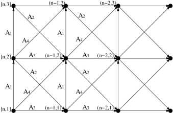
Figure 4: The recurrence relation for the Jacobi ensemble corresponds to lattice paths where $A_{1}$, $A_{2}$, $A_{3}$ and $A_{4}$ are respectively associated with vertical, falling, horizontal and rising steps.

We now have lattice paths with four possible steps: $(0,1)$, $(1,-1)$, $(1,0)$ and $(1,1)$ corresponding respectively to $A_{1}$, $A_{2}$, $A_{3}$ and $A_{4}$. The total displacement in the horizontal direction must be $n-1$. Let us consider the situations in which exactly $n-1-m$ of the horizontal moves come from $A_{3}$ steps. There are ${n-1\choose m}$ possibilities for assigning their position. Let us suppose that exactly $k$ of the remaining steps are of type $A_{4}$. We are thus reduced to counting the number of paths with $k$ raising steps, $m-k$ falling steps and $m-2k$ vertical steps. The key to this enumeration is that every one of these paths may be obtained from a Dyck path of length $2m-2k$, if we replace $m-2k$ of its raising steps by vertical ones. The number of such Dyck paths is $C_{m-k}$, and the number of possibilities to single out $m-2k$ of the raising steps is ${m-k\choose k}$.

In conclusion, the final result is given by

$$\langle T^{n}\rangle=A_{2}\sum_{m=0}^{n-1}{n-1\choose m}A_{3}^{n-1-m}\sum_{k=0}^{\left[\frac{m+1}{2}\right]}{m-k\choose k}C_{m-k}(-A_{1}A_{2})^{m-2k}(A_{4}A_{2})^{k}.$$ (60)

Replacing back $A_{4}$ by $A_{1}(1-A_{3})$ we arrive at the result (7). Naturally, when $\lim_{N\to\infty}\gamma/N=0$ we have $A_{3}=1$ and this reduces to (34).

References

• [1] Dyson, F.J.: Statistical theory of energy levels of complex systems I. J. Math. Phys. 3, 140- 156 (1962).
• [2] Kaneko, J.: Selberg integrals and hypergeometric functions associated with Jack polynomials. SIAM J. Math. Analysis, 24, 1086–1110 (1993).
• [3] Keating, J.P., Snaith, N.C.: Random matrix theory and $\zeta(1/2+it)$. Comm. Math. Phys. 214, 57- 89 (2001).
• [4] Di Francesco, P., Gaudin, M., Itzykson, C., Lesage, F.: Laughlin’s wave functions, Coulomb gases and expansions of the discriminant. Int. J. Mod. Phys. A 9, 4257–4351 (1994).
• [5] Beenakker, C.W.J.: Random matrix theory of quantum transport. Rev. Mod. Phys. 69, 731–808 (1997).
• [6] Forrester, P.J., Frankel, N.E., Garoni, T.M.: Random matrix averages and the impenetrable Bose gas in Dirichlet and Neumann boundary conditions. J. Math. Phys. 44, 4157-4175 (2003).
• [7] Mehta, M.L.: Random Matrices. New York: Academic Press, 2004.
• [8] Forrester, P.J.: Log-Gases and Random Matrices. Princeton: Princeton University Press, 2010.
• [9] Forrester, P.J., Warnaar, S.O.: The importance of the Selberg integral. Bull. Am. Math. Soc. 45, 489–534 (2008).
• [10] Forrester, P.J.: Quantum conductance problems and the Jacobi ensemble. J. Phys. A 39, 6861–6870 (2006).
• [11] Baranger, H.U., Mello, P.A.: Mesoscopic transport through chaotic cavities: A random S-matrix theory approach. Phys. Rev. Lett. 73, 142- 145 (1994).
• [12] Savin, D.V., Sommers, H.-J.: Shot noise in chaotic cavities with an arbitrary number of open channels, Phys. Rev. B 73, 081307 (2006).
• [13] Novaes, M.: Full counting statistics of chaotic cavities with many open channels. Phys. Rev. B 75, 073304 (2007).
• [14] Savin, D.V., Sommers, H.-J., Wieczorek, W.: Statistics of quantum transport in chaotic cavities with broken time-reversal symmetry. Phys. Rev. B 77, 125332 (2008).
• [15] Vivo, P., Vivo, E.: Transmission eigenvalue densities and moments in chaotic cavities from random matrix theory. J. Phys. A 41, 122004 (2008).
• [16] Novaes, M.: Statistics of quantum transport in chaotic cavities with broken time-reversal symmetry. Phys. Rev. B 78, 035337 (2008).
• [17] Kadell, K.W.J.: The Selberg-Jack symmetric functions, Adv. Math. 130, 33–102 (1997).
• [18] Khoruzhenko, B.A., Savin, D.V., Sommers, H.-J.: Systematic approach to statistics of conductance and shot-noise in chaotic cavities. Phys. Rev. B 80, 125301 (2009).
• [19] Luque, J.-G., Vivo, P.: Nonlinear random matrix statistics, symmetric functions and hyperdeterminants. J. Phys. A 43, 085213 (2010).
• [20] Brouwer, P.W., Beenakker, C.W.J.: Diagrammatic method of integration over the unitary group, with applications to quantum transport in mesoscopic systems. J. Math. Phys. 37, 4904–4934 (1996).
• [21] CarrΓ©, C., Deneufchatel, M., Luque, J.-G., Vivo, P.: Asymptotics of Selberg-like integrals: The unitary case and Newton’s interpolation formula, arXiv:1003.5996v1.
• [22] Brouwer, P.W., Frahm, K.M., Beenakker, C.W.J.: Quantum Mechanical Time-Delay Matrix in Chaotic Scattering. Phys. Rev. Lett. 78, 4737-4740 (1997).
• [23] Brouwer, P.W., Frahm, K.M., Beenakker, C.W.J.: Distribution of the quantum mechanical time-delay matrix for a chaotic cavity. Waves Random Media 9, 91–104 (1999).
• [24] Berkolaiko, G., Kuipers, J.: Moments of delay times. J. Phys. A 43, 035101 (2010).
• [25] Muirhead, R.J.: Aspects of Multivariate Statistical Theory, Chapter 3. Hoboken, Wiley, 2005.
• [26] Bai, Z.D, Yin, Z.Q., Krishnaiah, P.R.: On the limiting empirical distribution function of the eigenvalues of a multivariate F matrix. Theory Probab. Appl. 32, 490–500 (1985).
• [27] Aomoto, K.: Jacobi polynomials associated with Selberg integrals. SIAM J. Math. Analysis, 18, 545–549 (1987).