Hadron properties in AdS/QCD

Abstract

We discuss a holographic soft-wall model developed for the description of mesons and baryons with adjustable quantum numbers $n,J,L,S$. This approach is based on an action which describes hadrons with broken conformal invariance and which incorporates confinement through the presence of a background dilaton field. Results obtained for heavy-light meson masses and decay constants are consistent with predictions of HQET. In the baryon sector applications to the baryon masses, nucleon electromagnetic form factors and generalized parton distributions are discussed.

1 Introduction

Based on the correspondence of string theory in anti-de Sitter (AdS) space and conformal field theory (CFT) in physical space-time [1], a class of AdS/QCD approaches was recently successfully developed for describing the phenomenology of hadronic properties. In order to break conformal invariance and incorporate confinement in the infrared (IR) region two alternative AdS/QCD backgrounds have been suggested in the literature: the “hard-wall” approach [2], based on the introduction of an IR brane cutoff in the fifth dimension, and the “soft-wall” approach [3], based on using a soft cutoff. This last procedure can be introduced in the following ways: i) as a background field (dilaton) in the overall exponential of the action, ii) in the warping factor of the AdS metric, iii) in the effective potential of the action. These methods are in principle equivalent to each other due to a redefinition of the bulk field involving the dilaton field or by a redefinition of the effective potential. In the literature there exist detailed discussions of the sign of the dilaton profile in the dilaton exponential $\exp(\pm\varphi)$ [3, 4, 5, 6, 7] for the soft-wall model (for a discussion of the sign of the dilaton in the warping factor of the AdS metric see Refs. [8]). The negative sign was suggested in Ref. [3] and recently discussed in Ref. [7]. It leads to a Regge-like behavior of the meson spectrum, including a straightforward extension to fields of higher spin $J$. Also, in Ref. [7] it was shown that this choice of the dilaton sign guarantees the absence of a spurious massless scalar mode in the vector channel of the soft-wall model. We stress that alternative versions of this model with a positive sign are also possible. One should just redefine the bulk field $S(x,z)$ as $S(x,z)=e^{\varphi(z)}\,\tilde{S}(x,z)$, where the transformed field corresponds to the dilaton with an opposite profile. It is clear that the underlying action changes, and extra potential terms are generated depending on the dilaton field (see detailed discussion in [9]). Here we present a summary of recent results: meson mass spectrum and decay constants of light and heavy mesons, baryon masses, nucleon electromagnetic form factors and generalized parton distributions [9]-[11]. Our starting point are the effective $(d+1)$ dimensional actions formulated in AdS space in terms of boson or fermion bulk fields, which serve as holographic images of mesons and baryons.

2 Approach

Our starting point are the effective $(d+1)$ dimensional actions formulated in AdS space in terms of boson or fermion bulk fields, which serve as holographic images of mesons and baryons. For illustration we consider the simplest actions — for scalar fields ($J=0$) [10]-[12]

$$S_{0}=\frac{1}{2}\int d^{d}xdz\sqrt{g}e^{-\varphi(z)}\biggl{[}g^{MN}\partial_{M}S(x,z)\partial_{N}S(x,z)-\Big{(}\mu_{S}^{2}+\Delta V_{0}(z)\Big{)}\,S^{2}(x,z)\biggr{]}\,.$$ (1)

and $J=1/2$ fermions [13, 11]:

$$S_{1/2} = \int d^{d}xdz\,\sqrt{g}\,e^{-\varphi(z)}\,\biggl{[}\frac{i}{2}\bar{\Psi}(x,z)\epsilon_{a}^{M}\Gamma^{a}{\cal D}_{M}\Psi(x,z)-\frac{i}{2}({\cal D}_{M}\Psi(x,z))^{\dagger}\Gamma^{0}\epsilon_{a}^{M}\Gamma^{a}\Psi(x,z)$$ (2)

$$- \bar{\Psi}(x,z)\Big{(}\mu_{\Psi}+\varphi(z)/R)\Big{)}\Psi(x,z)\biggr{]}\,,$$

where $S$ and $\Psi$ are the scalar and fermion bulk fields, ${\cal D}_{M}$ is the covariant derivative acting on the fermion field, $\Gamma^{a}=(\gamma^{\mu},-i\gamma^{5})$ are the Dirac matrices, $\varphi(z)=\kappa^{2}z^{2}$ is the dilaton field, $R$ is the AdS radius, $\Delta V_{0}(z)$ is the dilaton potential. $\mu_{S}$ and $\mu_{\Psi}$ are the masses of scalar and fermion bulk fields defined as $\mu_{S}^{2}R^{2}=\Delta_{M}(\Delta_{M}-d)$ and $\mu_{\Psi}R=\Delta_{B}-d/2$. Here $\Delta_{M}=\tau_{M}=2+L$ and $\Delta_{B}=\tau_{B}+1/2=7/2+L$ are the dimensions of scalar and fermion fields, which due to the QCD/gravity correspondence are related to the scaling dimensions (twists $\tau_{M},\tau_{B}$) of the corresponding interpolating operators, where $L={\rm max}\,|L_{z}|$ [4] is the maximal value of the $z$-component of the quark orbital angular momentum in the LF wavefunction or the minimum of the orbital angular momentum of the corresponding hadron. These actions give information about the propagation of bulk fields inside AdS space (bulk-to-bulk propagators), from inside to the boundary of the AdS space (bulk-to-boundary propagators) and bound state solutions - profiles of the Kaluza-Klein (KK) modes in extra-dimension, which correspond to the hadronic wave functions in impact space. We suppose a free propagation of the bulk field along the $d$ Poincaré coordinates with four-momentum $p$, and a constrained propagation along the $(d+1)$-th coordinate $z$ (due to confinement imposed by the dilaton field). In particular, it was shown [4] that the extra-dimensional coordinate $z$ corresponds to the light-front impact variable. It was also shown [7] that in case of the scattering problem the sign of the dilaton profile is important to fulfill certain model-independent constraints. But we recently showed [9] that in case of the bound state problem the sign of the dilaton profile is irrelevant, if the action is properly set up. Moreover, in solving the bound-state problem, it is more convenient to move the dilaton field from the exponential prefactor to the effective potential [4, 9]. Then we use a KK expansion for the bulk fields factorizing the dependence on $d$ Poincaré coordinates $x$ and the holographic variable $z$. E.g. in case of scalar field it is given by $S(x,z)=\sum_{n}\ S_{n}(x)\ \Phi_{n}(z)$, where $n$ is the radial quantum number, $S_{n}(x)$ is the tower of the KK modes dual to scalar mesons and $\Phi_{n}$ are their extra-dimensional profiles (wave-functions) satisfying the Schrödinger-type equation with the potential depending on the dilaton field. Then using the obtained wave functions $\Phi_{n}$ we calculate matrix elements describing hadronic processes.

3 Results

We present the results of our calculations for mesonic decay constants (Table 1), the meson spectrum (Tables 2 and 3) [10] and the baryon spectrum (Tables 4 and 5). A detailed analysis of nucleon helicity-independent generalized parton distributions (GPDs) $H_{v}^{q}$ and $E_{v}^{q}$ [11] is discussed. Note, by construction we reproduce the power scaling of nucleon electromagnetic (EM) form factors at large $Q^{2}$ [13, 11]:

$$F_{1}^{p}(Q^{2}) = C_{1}(Q^{2})+\eta_{p}C_{2}(Q^{2})\,,$$

$$F_{2}^{p}(Q^{2}) = \eta_{p}C_{3}(Q^{2})\,,$$

$$F_{1}^{n}(Q^{2}) = \eta_{n}C_{2}(Q^{2})\,,$$

$$F_{2}^{n}(Q^{2}) = \eta_{n}C_{3}(Q^{2}),$$

where $Q^{2}=-t$. The $C_{i}$ functions, defining the Dirac and Pauli factors, are given by:

$$C_{1}(Q^{2}) = \frac{a+6}{(a+1)(a+2)(a+3)}\,,$$

$$C_{2}(Q^{2}) = \frac{2a(2a-1)}{(a+1)(a+2)(a+3)(a+4)}\,,$$ (4)

$$C_{3}(Q^{2}) = \frac{12m_{N}\sqrt{2}}{\kappa}\,\frac{1}{(a+1)(a+2)(a+3)}\,,$$

where $a=Q^{2}/(4\kappa^{2})$. Note that we obtain the correct scaling behavior of the nucleon form factors at large $Q^{2}$, $F_{1}^{p,n}\sim 1/Q^{4}$ and $F_{2}^{p,n}\sim 1/Q^{6}$.

Our predictions for the EM radii compare well with data:

$$\langle r^{2}_{E}\rangle^{p}=0.91\ {\rm fm}^{2}\ {\rm(our)}\,,\ 0.77\ {\rm fm}^{2}\ {\rm(data)}\,;\ \langle r^{2}_{E}\rangle^{n}=-0.12\ {\rm fm}^{2}\ {\rm(our)}\,,\ -0.12\ {\rm fm}^{2}\ {\rm(data)}\,,$$

$$\langle r^{2}_{M}\rangle^{p}=0.85\ {\rm fm}^{2}\ {\rm(our)}\,,\ 0.73\ {\rm fm}^{2}\ {\rm(data)}\,;\ \langle r^{2}_{M}\rangle^{n}=0.88\ {\rm fm}^{2}\ {\rm(our)}\,,\ 0.76\ {\rm fm}^{2}\ {\rm(data)}\,.$$

In the following we discuss in detail our results for GPDs, which are related to the electromagnetic form factors via sum rules [14, 15]. In particular, in momentum space $H_{v}^{q}$ and $E_{v}^{q}$ are given by

$$H_{v}^{q}(x,Q^{2}) = q(x)\,x^{a}\,,$$ (5)

$$E_{v}^{q}(x,Q^{2}) = e^{q}(x)\,x^{a}\,.$$ (6)

Here $q(x)$ and $e^{q}(x)$ are distribution functions given by:

$$q(x)=\alpha^{q}\gamma_{1}(x)+\beta^{q}\gamma_{2}(x)\,,\quad e^{q}(x)=\beta^{q}\gamma_{3}(x)\,,$$ (7)

where the flavor couplings $\alpha^{q},\beta^{q}$ and functions $\gamma_{i}(x)$ are written as

$$\alpha^{u}=2\,,\ \alpha^{d}=1\,,\ \beta^{u}=2\eta_{p}+\eta_{n}\,,\ \beta^{d}=\eta_{p}+2\eta_{n}\,$$ (8)

and

$$\gamma_{1}(x) = \frac{1}{2}(5-8x+3x^{2})\,,$$

$$\gamma_{2}(x) = 1-10x+21x^{2}-12x^{3}\,,$$ (9)

$$\gamma_{3}(x) = \frac{6m_{N}\sqrt{2}}{\kappa}(1-x)^{2}\,.$$

The parameters are $\kappa=350$ MeV, $\eta_{p}=0.224$, $\eta_{n}=-0.239$, which were fixed in order to reproduce the mass $m_{N}=2\kappa\sqrt{2}$ and the anomalous magnetic moments of the nucleon $k_{p}=\mu_{p}-1=1.791$ and $k_{n}=\mu_{n}=-1.913$. The plots of the GPDs in momentum space are presented in Fig.1.

Another interesting aspect to consider are the nucleon GPDs in impact space. As shown in [16], the GPDs in momentum space are related to the impact parameter dependent parton distributions by a Fourier transform. GPDs in impact space give access to the distribution of partons in the transverse plane, which is quite important for understanding the nucleon structure. Soft-wall AdS/QCD gives the following predictions for the impact space properties of nucleons:

$$q(x,{\bf b}_{\perp}) = q(x)\frac{\kappa^{2}}{\pi\log(1/x)}e^{-\frac{{\bf b}_{\perp}^{2}\kappa^{2}}{\log(1/x)}}\,,$$

$$e^{q}(x,{\bf b}_{\perp}) = e^{q}(x)\frac{\kappa^{2}}{\pi\log(1/x)}e^{-\frac{{\bf b}_{\perp}^{2}\kappa^{2}}{\log(1/x)}}\,,$$

$$\rho_{E}^{N}({\bf b}_{\perp}) = \frac{\kappa^{2}}{\pi}\sum\limits_{q}e_{q}^{N}\int\limits_{0}^{1}\frac{dx}{\log(1/x)}q(x)e^{-\frac{{\bf b}_{\perp}^{2}\kappa^{2}}{\log(1/x)}}\,,$$

$$\rho_{M}^{N}({\bf b}_{\perp}) = \frac{\kappa^{2}}{\pi}\sum\limits_{q}e_{q}^{N}\int\limits_{0}^{1}\frac{dx}{\log(1/x)}e^{q}(x)e^{-\frac{{\bf b}_{\perp}^{2}\kappa^{2}}{\log(1/x)}}\,,$$

$$\langle R_{\perp}^{2}(x)\rangle_{q} = \frac{\log(1/x)}{\kappa^{2}}\,,$$

$$\langle R_{\perp}^{2}\rangle_{q} = \frac{1}{\kappa^{2}}\biggl{(}\frac{5}{3}+\frac{\beta^{q}}{12\alpha^{q}}\biggr{)}\,.$$ (10)

Fig.3 shows some examples of $q(x,{\bf b}_{\perp})$ and in Fig.4 we plot $\rho_{E}^{N}({\bf b}_{\perp})$ and $\rho_{M}^{N}({\bf b}_{\perp})$ for proton and neutron. For the transverse rms radius of $u-$ and $d-$quark GPDs we get similar values:

$$\langle R_{\perp}^{2}\rangle_{u}=0.527\ {\rm fm}^{2}\,,\quad\langle R_{\perp}^{2}\rangle_{d}=0.524\ {\rm fm}^{2}\,.$$ (11)

One should stress that the obtained nucleon GPDs both in momentum and impact spaces correspond to the so-called “Gaussian ansatz” and are consistent with general predictions for their asymptotic behavior for $x\to 0$ or $x\to 1$ and $Q^{2}\to 0$ or $Q^{2}\to\infty$. The plots of GPDs in impact space are given in Fig.2.

Table 1. Decay constants $f_{P}$ (MeV) of pseudoscalar mesons

Meson	Data	Our
$\pi^{-}$	$130.4\pm 0.03\pm 0.2$	131
$K^{-}$	$156.1\pm 0.2\pm 0.8$	155
$D^{+}$	$206.7\pm 8.9$	167
$D_{s}^{+}$	$257.5\pm 6.1$	170
$B^{-}$	$193\pm 11$	139
$B_{s}^{0}$	$253\pm 8\pm 7$	144

Table 2. Masses of light mesons in MeV

Meson	$n$	$L$	$S$	Mass
$\pi$	0	0,1,2,3	0	$140$	$1355$	$1777$	$2099$
$\pi$	0,1,2,3	0	0	$140$	$1355$	$1777$	$2099$
$K$	0	0,1,2,3	$\;0\;$	$496$	$1505$	$1901$	$2207$
$f_{0}[\bar{n}n]$	0,1,2,3	1	1	$1114$	$1600$	$1952$	$2244$
$f_{0}[\bar{s}s]$	0,1,2,3	1	1	$1304$	$1762$	$2093$	$2372$
$a_{0}(980)$	0,1,2,3	1	1	$1114$	$1600$	$1952$	$2372$
$\rho(770)$	0,1,2,3	0	1	$804$	$1565$	$1942$	$2240$
$\phi(1020)$	0,1,2,3	0	1	$1019$	$1818$	$2170$	$2447$
$a_{1}(1260)$	0,1,2,3	1	1	$1358$	$1779$	$2101$	$2375$

Table 3. Masses of heavy-light mesons in MeV

Meson	$J^{\rm P}$	$n$	$L$	$S$	Mass
$D(1870)$	$0^{-}$	0	0,1,2,3	0	1857	2435	2696	2905
$D^{\ast}(2010)$	$1^{-}$	0	0,1,2,3	1	2015	2547	2797	3000
$D_{s}(1969)$	$0^{-}$	0	0,1,2,3	0	1963	2621	2883	3085
$D^{\ast}_{s}(2107)$	$1^{-}$	0	0,1,2,3	1	2113	2725	2977	3173
$B(5279)$	$0^{-}$	0	0,1,2,3	0	5279	5791	5964	6089
$B^{\ast}(5325)$	$1^{-}$	0	0,1,2,3	1	5336	5843	6015	6139
$B_{s}(5366)$	$0^{-}$	0	0,1,2,3	0	5360	5941	6124	6250
$B^{\ast}_{s}(5413)$	$1^{-}$	0	0,1,2,3	1	5416	5992	6173	6298

Table 4. Masses of light baryons in MeV

Baryon	Our results	Data
$N$	939	939
$\Lambda$	1114	1116
$\Sigma$	1180	1189
$\Xi$	1328	1322
$\Delta$	1232	1232
$\Sigma^{\ast}$	1381	1385
$\Xi^{\ast}$	1533	1530
$\Omega$	1688	1672

Table 5. Masses of $N$ and $\Delta$ families in MeV

Baryon	Our results	Data
$N_{1/2^{+}}(939)$	939	939
$N_{1/2^{+}}(1440)$	1372	$1440^{+30}_{-20}$
$N_{1/2^{+}}(1710)$	1698	$1710\pm 30$
$N_{1/2^{+}}(1880)$	1970
$N_{1/2^{+}}(2100)$	2209
$\Delta_{3/2^{+}}(1232)$	1232	$1232$
$\Delta_{3/2^{+}}(1600)$	1587	$1600^{+100}_{-50}$
$\Delta_{3/2^{+}}(1920)$	1876	$1920^{+50}_{-20}$

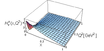
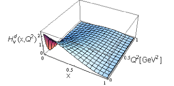
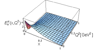
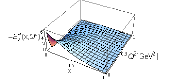
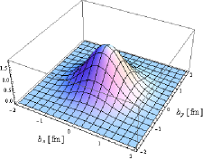
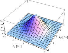
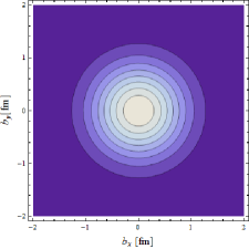
Figure 1: Nucleon helicity-independent GPDs in momentum space

Figure 2: Nucleon helicity-independent GPDs in impact space. Plots for $q(x,{\bf b}_{\perp})$ for $x=0.1$: $u(x,{\bf b}_{\perp})$ - upper pannels, $d(x,{\bf b}_{\perp})$ - lower pannels

4 Conclusion

We present a summary of recent results obtained in a soft-wall model based on the gauge/gravity duality: meson mass spectrum and decay constants of light and heavy mesons, baryon masses, nucleon electromagnetic form factors and generalized parton distributions.

Acknowledgements

The authors thank Stan Brodsky and Guy de Téramond for useful discussions and remarks. This work was supported by Federal Targeted Program “Scientific and scientific-pedagogical personnel of innovative Russia” Contract No. 02.740.11.0238, by FONDECYT (Chile) under Grant No. 1100287. A.V. acknowledges the financial support from FONDECYT (Chile) Grant No. 3100028. V.E.L. would like to thank Departamento de Física y Centro Científico Tecnológico de Valparaíso (CCTVal), Universidad Técnica Federico Santa María, Valparaíso, Chile for warm hospitality.

References

• [1] J. M. Maldacena, Adv. Theor. Math. Phys. 2 (1998) 231 ; S. S. Gubser, I. R. Klebanov and A. M. Polyakov, Phys. Lett. B 428 (1998) 105 ; E. Witten, Adv. Theor. Math. Phys. 2 (1998) 253 .
• [2] J. Polchinski, M. J. Strassler, Phys. Rev. Lett. 88 (2002) 031601 .
• [3] A. Karch, E. Katz, D. T. Son and M. A. Stephanov, Phys. Rev. D 74 (2006) 015005 .
• [4] S. J. Brodsky, G. F. de Teramond, Phys. Rev. Lett. 96 (2006) 201601 ; Phys. Rev. D 77 (2008) 056007 ; G. F. de Teramond, S. J. Brodsky, Nucl. Phys. Proc. Suppl. 199 (2010) 89 .
• [5] G. F. de Teramond and S. J. Brodsky (2010). AIP Conf. Proc. 1296 (2010) 128 .
• [6] F. Zuo, Phys. Rev. D 82 (2010) 086011 ; S. Nicotri, AIP Conf. Proc. 1317 (2011) 322 .
• [7] A. Karch, E. Katz, D. T. Son, M. A. Stephanov, JHEP 1104 (2011) 066 .
• [8] O. Andreev, Phys. Rev. D 73 (2006) 107901 ; H. Forkel, M. Beyer and T. Frederico, JHEP 0707 (2007) 077 .
• [9] T. Gutsche, V. E. Lyubovitskij, I. Schmidt and A. Vega, arXiv:1108.0346 [hep-ph].
• [10] T. Branz, T. Gutsche, V. E. Lyubovitskij, I. Schmidt, A. Vega, Phys. Rev. D 82 (2010) 074022 .
• [11] A. Vega, I. Schmidt, T. Gutsche, V. E. Lyubovitskij, Phys. Rev. D 83 (2011) 036001 .
• [12] A. Vega and I. Schmidt, Phys. Rev. D 78 (2008) 017703 ; A. Vega and I. Schmidt, Phys. Rev. D 79 (2009) 055003 ; A. Vega, I. Schmidt, T. Branz, T. Gutsche and V. E. Lyubovitskij, Phys. Rev. D 80 (2010) 055014 ; A. Vega, I. Schmidt, Phys. Rev. D 82 (2010) 115023 .
• [13] Z. Abidin and C. E. Carlson, Phys. Rev. D 79 (2009) 115003 .
• [14] X. D. Ji, Phys. Rev. D 55 (1997) 7114 .
• [15] A. V. Radyushkin, Phys. Rev. D 56 (1997) 5524 .
• [16] M. Burkardt, Phys. Rev. D 62 (2000) 071503 [Erratum-ibid. Phys. Rev. D 66 (2002) 119903 ]; Int. J. Mod. Phys. A 18 (2003) 173 .