ORTHOGONAL POLYNOMIALS OF THE $\mathbb{R}$-LINEAR GENERALIZED MINIMAL RESIDUAL METHOD

Abstract

The speed of convergence of the $\mathbb{R}$-linear GMRES method is bounded in terms of a polynomial approximation problem on a finite subset of the spectrum. This result resembles the classical GMRES convergence estimate except that the matrix involved is assumed to be condiagonalizable. The bounds obtained are applicable to the CSYM method, in which case they are sharp. Then a three term recurrence for generating a family of orthogonal polynomials is shown to exist, yielding a natural link with complex symmetric Jacobi matrices. This shows that a mathematical framework analogous to the one appearing with the Hermitian Lanczos method exists in the complex symmetric case. The probability of being condiagonalizable is estimated with random matrices.

1 Introduction

Suggested in [9], there exists an $\mathbb{R}$-linear GMRES (generalized minimal residual) method for solving a large real linear system of equations of the form

$$\kappa z+{M_{\scriptscriptstyle\#}}\overline{z}=b$$ (1)

for $\kappa\in\,\mathbb{C}$, ${M_{\scriptscriptstyle\#}}\in\,\mathbb{C}^{n\times n}$ and $b\in\,\mathbb{C}^{n}$. Systems of this type appear regularly in applications. This is manifested by the complex symmetric case which corresponds to $\kappa=0$ and ${M_{\scriptscriptstyle\#}}^{T}={M_{\scriptscriptstyle\#}}$. (For its importance in applications, such as the numerical solution of the complex Helmholtz equation, see [11].) Then the $\mathbb{R}$-linear GMRES method reduces to the CSYM method [5]. We have $\kappa\not=0$, e.g., in an approach to solve the electrical conductivity problem [2] which requires solving an $\mathbb{R}$-linear Beltrami equation [21]. For a wealth of information regarding real linearity, see [22, 7]. Although the $\mathbb{R}$-linear GMRES method is a natural scheme, its properties are not well understood. Assuming ${M_{\scriptscriptstyle\#}}$ to be condiagonalizable, in this paper a polynomial approximation problem on the plane is introduced for assessing its speed of convergence. In the complex symmetric case a three term recurrence for generating orthogonal polynomials arises, leading to a natural link with complex symmetric Jacobi matrices.

The bounds obtained are intriguing by the fact that they show that the convergence depends on the spectrum of the real linear operator involved. So far it has not been clear what is the significance of the spectrum in general and for iterative methods in particular [17, 9]. Here it is shown to play a role similar to what the spectrum does in the classical GMRES bounds [29]. A striking difference is that the bounds reveal a strong dependence of the speed of convergence on the vector.

Moreover, with any natural Krylov subspace method there exists a connection between the iteration and orthogonal functions. As a rule, these are associated with normality. The Hermitian Lanczos method is related with a three term recurrence for generating orthogonal polynomials; see [15] and references therein. For unitary matrices the corresponding length of recurrence is five [28]; see also [30]. These are special instances of the general framework for normal matrices described in [18, 19]. In this paper an analogous connection is established in the complex symmetric case to orthogonalize monomials

$$1,\,\lambda,\,|\lambda|^{2},\,\lambda|\lambda|^{2},\,|\lambda|^{4},\,\lambda|\lambda|^{4},\ldots$$ (2)

with a three term recurrence. This link is not entirely unexpected by the fact that antilinear operators involving a complex symmetric matrix ${M_{\scriptscriptstyle\#}}$ have been regarded as yielding an analogue of normality [17, p. 250]. As opposed to the Hermitian Lanczos method, the structure is richer now as orthogonality based on a three term recurrence and respective rapid least squares approximation is possible on very peculiar curves in $\,\mathbb{C}$ (and not just on subsets of $\mathbb{R}$ which are also admissible); see the assumptions of Theorem 16 for the admissible curves. The arising family of functions can be viewed to extend radial functions in a natural way.

Unlike diagonalizability in the complex linear case, condiagonalizability is a more intricate structure. Random matrix theory is invoked to assess how likely it is to have a condiagonalizable operator in (1). In this manner we end up touching many aspects of the theory that has been linked by the classical Hermitian Lanczos method in recent years [6].

The paper is organized as follows. In Section 2 bounds on the $\mathbb{R}$-linear GMRES convergence are derived in the condiagonalizable case. The probability of a matrix being condiagonalizable is assessed in Section 3. Section 4 is concerned with the theory of orthogonal polynomials related with the $\mathbb{R}$-linear Arnoldi method. It is shown that complex symmetry is naturally treated within antilinear structure. Only then its rich properties become visible. In Section 5 some preliminary numerical experiments are presented.

2 Condiagonalizability and the convergence of the $\mathbb{R}$-linear GMRES

Condiagonalizability means that the real linear operator appearing on the left-hand side of (1) is diagonalizable. Before deriving the bounds, we first recall how Krylov subspaces are generated with an $\mathbb{R}$-linear operator in (1) by executing the $\mathbb{R}$-linear Arnoldi method.

2.1 Krylov subspaces of the $\mathbb{R}$-linear GMRES

When $\,\mathbb{C}^{n}$ is regarded as a vector space over $\,\mathbb{C}$, any real linear operator can be presented as

$$z\longmapsto\mathcal{M}z=(M+{M_{\scriptscriptstyle\#}}\tau)z=Mz+{M_{\scriptscriptstyle\#}}\overline{z}$$ (3)

with matrices $M,{M_{\scriptscriptstyle\#}}\in\,\mathbb{C}^{n\times n}$. Here $\tau$ denotes the conjugation operator on $\,\mathbb{C}^{n}$. The set of eigenvalues, i.e., the spectrum of a real linear operator $\mathcal{M}=M+{M_{\scriptscriptstyle\#}}\tau$ is defined as

$$\left\{{\lambda\in\,\mathbb{C}}\,\big{|}\,{\mathcal{M}z=\lambda z\,\mbox{ for some }\,z\not=0}\right\}.$$

The spectrum is an algebraic set of degree $2n$ at most. For more details on the real linear eigenvalue problem, see [9, 20].

In this paper we are interested in having $M=\kappa I$ for a scalar $\kappa\in\,\mathbb{C}$. Then the real linear operator is denoted by $\mathcal{M}_{\kappa}$. In this case the spectrum possesses a relatively simple structure as follows.

Proposition 1.

The spectrum of $\mathcal{M}_{\kappa}$ consists of circles centred at $\kappa$.

The eigenvalues of $\mathcal{M}_{0}$, i.e., circles centred at the origin, are also called the coneigenvalues of the matrix ${M_{\scriptscriptstyle\#}}$ [17].

To describe methods to compute Krylov subspaces with $\mathbb{R}$-linear operators, we follow [9, Section 3.1]. Executing the iteration with $\mathcal{M}_{\kappa}$ starting from a vector $b\in\,\mathbb{C}^{n}$, we obtain the Krylov subspace

$$\mathcal{K}_{j}(\mathcal{M}_{\kappa};b)={\rm span}\{b,\mathcal{M}_{\kappa}b,\ldots,\mathcal{M}_{\kappa}^{j-1}b\}$$

$$={\rm span}\{b,{M_{\scriptscriptstyle\#}}\overline{b},{M_{\scriptscriptstyle\#}}\overline{{M_{\scriptscriptstyle\#}}}b,{M_{\scriptscriptstyle\#}}\overline{{M_{\scriptscriptstyle\#}}}{M_{\scriptscriptstyle\#}}\overline{b},\ldots\}$$

which is hence independent of $\kappa$. For this an orthonormal basis can be computed numerically reliably by invoking the real linear Arnoldi method [9, p. 820]. In particular, if $\dim\mathcal{K}_{j}(\mathcal{M}_{\kappa};b)=n$ and $Q$ denotes the respective unitary matrix having the orthonormal basis vectors as its columns, then $Q^{*}{M_{\scriptscriptstyle\#}}\overline{Q}\tau$ is the respective representation of ${M_{\scriptscriptstyle\#}}\tau$ in this basis.

The following simple fact is of importance.

Proposition 2.

Let $X\in\,\mathbb{C}^{n\times n}$ be invertible. Then

$$X^{-1}\mathcal{K}_{j}(\mathcal{M}_{\kappa};b)=\mathcal{K}_{j}(\mathcal{N}_{\kappa};c)$$

with ${N_{\scriptscriptstyle\#}}=X^{-1}{M_{\scriptscriptstyle\#}}\overline{X}$ and $c=X^{-1}b$.

If $X$ is unitary, then the corresponding sequences of Krylov subspaces are indistinguishable in the standard Euclidean geometry, i.e., all the corresponding inner products computed coincide.

In the $\mathbb{R}$-linear GMRES method for solving (1) suggested in [9], at the $j$th step one imposes the minimum residual condition

$$\min_{z\in\mathcal{K}_{j}(\mathcal{M}_{\kappa};b)}\left|\left|\mathcal{M}_{\kappa}z-b\right|\right|$$

for the approximation to satisfy. With appropriate modifications taking into account the real linearity, the iteration can be implemented to proceed like the classical GMRES [29]. In particular, if ${M_{\scriptscriptstyle\#}}$ is either symmetric or skew-symmetric, then the iteration can be realized in terms of a three term recurrence.

It is noteworthy that the $\mathbb{R}$-linear GMRES converges at least as fast as the standard GMRES applied to the real system of doubled size obtained by separating the real and imaginary parts in (1). This fact is not surprising. For Krylov subspace methods, not writing complex problems in a real form has been advocated already in [11, p. 446]. Thereby understanding the convergence of the $\mathbb{R}$-linear GMRES is of central relevance.

As a final remark, to precondition the linear system (1) such that the structure is preserved, see [21, Section 4.2].

2.2 Polynomial approximation problem of the $\mathbb{R}$-linear GMRES convergence

The following notion is needed in what follows.

Definition 3.

A matrix ${M_{\scriptscriptstyle\#}}\in\,\mathbb{C}^{n\times n}$ is said to be condiagonalizable if there exists an invertible matrix $X\in\,\mathbb{C}^{n\times n}$ such that

$${M_{\scriptscriptstyle\#}}=X{\Lambda_{\scriptscriptstyle\#}}\overline{X^{-1}}$$ (4)

with a diagonal matrix ${\Lambda_{\scriptscriptstyle\#}}$.

The diagonal entries of ${\Lambda_{\scriptscriptstyle\#}}$ are also called the coneigenvalues of ${M_{\scriptscriptstyle\#}}$. (Admittedly, there is a minor, although trivial inconsistency here compared with the comment following Proposition 1.)

Analytic polynomials are not sufficient to deal with real linear operators. The following subclass of (polyanalytic) polynomials is of central relevance for the $\mathbb{R}$-linear GMRES.

Definition 4.

Polynomials of the form

$$\sum_{k=0}^{\lfloor\frac{j}{2}\rfloor}(\alpha_{2k}+\alpha_{2k+1}\lambda)\left|\lambda\right|^{2k}$$ (5)

with $\alpha_{k}\in\,\mathbb{C}$ and, for $j$ even $\alpha_{j+1}=0$, are denoted by $\mathcal{P}_{j}(r2)$. Their union $\cup_{j=0}^{\infty}\mathcal{P}_{j}(r2)$ is denoted by $\mathcal{P}(r2).$

Clearly, $\mathcal{P}_{j}(r2)$ is a vector space over $\,\mathbb{C}$ of dimension $j+1$. With the restriction $\lambda\in\mathbb{R}$ we are dealing with standard analytic polynomials. It is, however, more natural to contrast $\mathcal{P}_{j}(r2)$ with radial functions. This and the notation used will be explained Section 4.2.

Observe that problems involving the conjugated variable are becoming more common in applications. Gravitational lensing is one such instance [24].

Like in the standard GMRES polynomial approximation problem, it is critical how well a nonzero constant can be approximated with the elements of $\mathcal{P}_{j}(r2)$. As usual, we denote the condition number of a matrix $X\in\,\mathbb{C}^{n\times n}$ by $\kappa_{2}(X)=\left|\left|X\right|\right|\left|\left|X^{-1}\right|\right|.$

Theorem 5.

Suppose ${M_{\scriptscriptstyle\#}}\in\,\mathbb{C}^{n\times n}$ is condiagonalizable as (4). If $D$ is a unitary diagonal matrix satisfying $D^{-1}X^{-1}b\in\mathbb{R}^{n}$, then

$$\min_{z\in\mathcal{K}_{j}(\mathcal{M}_{\kappa};b)}\left|\left|\mathcal{M}_{\kappa}z-b\right|\right|\leq\kappa_{2}(X)\min_{p\in\mathcal{P}_{j-1}(r2)}\max_{\lambda\in\sigma({D_{\scriptscriptstyle\#}})}\left|\kappa p(\lambda)+\lambda\overline{p(\lambda)}-1\right|\left|\left|b\right|\right|,$$

where ${D_{\scriptscriptstyle\#}}$ denotes the diagonal matrix $D^{-1}{\Lambda_{\scriptscriptstyle\#}}\overline{D}$.

Proof.

Recall that $\mathcal{K}_{j}(\mathcal{M}_{\kappa};b)=\mathcal{K}_{j}(\mathcal{M}_{0};b)$ holds for any $\kappa\in\,\mathbb{C}$. Take any $z\in\mathcal{K}_{j}(\mathcal{M}_{0};b)$ and set $w=D^{-1}X^{-1}z$. Denote $D^{-1}X^{-1}b$ by $r$. Since the vector $r$ is real, we obtain

$$w=D^{-1}X^{-1}z=D^{-1}X^{-1}(\sum_{k=0}^{j-1}\alpha_{k}\mathcal{M}_{0}^{k}b)=\sum_{k=0}^{j-1}\alpha_{k}\mathcal{D}_{0}^{k}(D^{-1}X^{-1}b)=\sum_{k=0}^{j-1}\alpha_{k}\mathcal{D}_{0}^{k}r$$

$$=\sum_{k=0}^{\lfloor\frac{j-1}{2}\rfloor}(\alpha_{2k}+\alpha_{2k+1}{D_{\scriptscriptstyle\#}})({D_{\scriptscriptstyle\#}}\overline{{D_{\scriptscriptstyle\#}}})^{k}r$$

for some constants $\alpha_{k}\in\,\mathbb{C}$ with and $\alpha_{2\lfloor(j-1)/2\rfloor+1}=0$ for $j$ odd. This is a polynomial in a diagonal, i.e., normal matrix and its adjoint. Hence we have obtained a link between polynomials in $\lambda$ and $\overline{\lambda}$. Now we have

$$\left|\left|\mathcal{M}_{\kappa}z-b\right|\right|\leq\left|\left|XD\right|\right|\left|\left|\mathcal{D}_{\kappa}w-r\right|\right|=\left|\left|XD\right|\right|\left|\left|\kappa w+{D_{\scriptscriptstyle\#}}\overline{w}-r\right|\right|.$$

Then again, since the vector $r$ is real,

$$\left|\left|\kappa w+{D_{\scriptscriptstyle\#}}\overline{w}-r\right|\right|\leq$$

$$\left|\left|(\kappa\sum_{k=0}^{\lfloor\frac{j-1}{2}\rfloor}(\alpha_{2k}+\alpha_{2k+1}{D_{\scriptscriptstyle\#}})({D_{\scriptscriptstyle\#}}\overline{{D_{\scriptscriptstyle\#}}})^{k}+{D_{\scriptscriptstyle\#}}\overline{\sum_{k=0}^{\lfloor\frac{j-1}{2}\rfloor}(\alpha_{2k}+\alpha_{2k+1}{D_{\scriptscriptstyle\#}})({D_{\scriptscriptstyle\#}}\overline{{D_{\scriptscriptstyle\#}}})^{k}}-I)r\right|\right|$$

$$\leq\max_{\lambda\in\sigma({D_{\scriptscriptstyle\#}})}\left|\kappa p(\lambda)+\lambda\overline{p(\lambda)}-1\right|\left|\left|(DX)^{-1}\right|\right|\left|\left|b\right|\right|$$

where $p$ belongs to $\mathcal{P}_{j-1}(r2)$. Since $\left|\left|XD\right|\right|\left|\left|(XD)^{-1}\right|\right|=\kappa_{2}(X)$, the claim follows from this. ∎

Observe that in $D^{-1}{\Lambda_{\scriptscriptstyle\#}}\overline{D}$ the $j$th diagonal entry of ${\Lambda_{\scriptscriptstyle\#}}$ has been multiplied by $e^{-2i\theta_{j}}$, where $e^{i\theta_{j}}$ is the $j$th diagonal entry of $D$.

The key here is the fact that the latter minimisation problem is of standard type. Being part of classical approximation theory of functions, there is no linear algebra involved. However, unlike the usual GMRES bound [29, Section 3.4], the point set $\sigma({D_{\scriptscriptstyle\#}})$ depends strikingly on the vector $b$. (The choice of $D$ to make $X^{-1}b$ real depends on $b$.) It is a finite subset of the spectrum consisting of at most $n$ points, though. Generically these points are unique. (Generic here means that ${M_{\scriptscriptstyle\#}}$, when condiagonalizable, is assumed to have distinct coneigenvalues.) Moreover, for an appropriate choice of $b$, it can be any subset of the spectrum with the restriction that the number coneigenvalues of ${M_{\scriptscriptstyle\#}}$ of the same modulus does not change.

The bound shows also that the notion of “spectral radius” for a diagonalizable antilinear operator is natural. Observe that, by executing the real linear Arnoldi method, it is straightforward to estimate the extreme coneigenvalues of a large (and possibly sparse) ${M_{\scriptscriptstyle\#}}$. The rationale is analogous to the way the classical Arnoldi method yields eigenvalue approximations.

The convergence behaviour of the CSYM method has been regarded as somewhat puzzling as well, partly because of the somewhat unaccesible structure of the appearing Krylov subspaces. For some comparisons between other iterative methods, see [5, 23]. (Lack of understanding the convergence is not just of theoretical interest. It can prevent efficient preconditioning.) The following yields a way to look at it.

Corollary 6.

For the CSYM method we can choose $X$ to be unitary to have

$$\min_{z\in\mathcal{K}_{j}(\mathcal{M}_{0};b)}\left|\left|\mathcal{M}_{0}z-b\right|\right|\leq\min_{p\in\mathcal{P}_{j-1}(r2)}\max_{\lambda\in\sigma({D_{\scriptscriptstyle\#}})}\left|\lambda\overline{p(\lambda)}-1\right|\left|\left|b\right|\right|,$$

where ${D_{\scriptscriptstyle\#}}=D^{-1}{\Lambda_{\scriptscriptstyle\#}}\overline{D}$.

These bounds are clearly sharp [16].

Observe that if $\sigma({D_{\scriptscriptstyle\#}})$ is on a line through the origin, then the CSYM method reduces to the MINRES (minimal residual) method [26] for Hermitian matrices. In this case the convergence can be regarded as well understood. For instance, then the convergence can be expected to be faster if the origin is not included in the convex hull of the spectrum. The difference can be dramatic as well.

3 The probability of condiagonalizability

In complex linear matrix analysis, a linear operator is diagonalizable with probability one. Therefore the analysis of the speed of convergence of iterations based on classical approximation theory of functions on the spectrum is generically a viable approach. In a typical case it can be expected to yield good estimates.

Although the set of condiagonalizable matrices includes complex symmetric matrices, a subspace of $\,\mathbb{C}^{n\times n}$ of dimension $n(n+1)/2$, assuming condiagonalizability turns out to be much more restrictive than assuming diagonalizability. Quantitatively this can be expressed in terms of the following result on random matrices.

Theorem 7.

Let ${M_{\scriptscriptstyle\#}}\in{\mathbb{C}}^{n\times n}$ have entries with real and imaginary parts drawn independently from the standard normal distribution. Then the probability that ${M_{\scriptscriptstyle\#}}$ is condiagonalizable is $2^{-n(n-1)/2}$.

One should bear in mind that in practice matrices possess a lot of structure (such as complex symmetry). Thereby, regarding the usage of the bounds of Section 2 in applications, this is certainly an overly pessimistic result.

The rest of this section is dedicated to the proof of Theorem 7. The probability that a real $n$-by-$n$ matrix with standard normal entries has only real eigenvalues has been shown to equal $2^{-n(n-1)/4}$ [8]. From Proposition 9 below it is easy to see that a real matrix is condiagonalizable with the same probability. For the complex matrices of Theorem 7, our computation of the probability proceeds similarly to [8].

3.1 Contriangularizable matrices

We start by recalling basic facts on matrices and consimilarity needed in the proof. A standard reference here is [17, Chapter 4].

Definition 8.

A matrix ${M_{\scriptscriptstyle\#}}\in\,\mathbb{C}^{n\times n}$ is said to be contriangularizable if there exists an invertible matrix $X\in\,\mathbb{C}^{n\times n}$ such that

$${M_{\scriptscriptstyle\#}}=X{R_{\scriptscriptstyle\#}}\overline{X^{-1}}$$ (6)

with an upper triangular matrix ${R_{\scriptscriptstyle\#}}$.

A matrix ${M_{\scriptscriptstyle\#}}$ is said to be unitarily contriangularizable if ${M_{\scriptscriptstyle\#}}=U{R_{\scriptscriptstyle\#}}U^{T}$ with $U$ unitary and ${R_{\scriptscriptstyle\#}}$ upper triangular.

Proposition 9.

Suppose ${M_{\scriptscriptstyle\#}}\in{\mathbb{C}}^{n\times n}$. Then

1. ${M_{\scriptscriptstyle\#}}$ is contriangularizable if and only if ${M_{\scriptscriptstyle\#}}$ is unitarily contriangularizable if and only if all the eigenvalues of ${M_{\scriptscriptstyle\#}}\overline{{M_{\scriptscriptstyle\#}}}$ are real and nonnegative.

2. if ${M_{\scriptscriptstyle\#}}=U{R_{\scriptscriptstyle\#}}U^{T}$ with $U$ unitary and ${R_{\scriptscriptstyle\#}}$ upper triangular, the absolute values of the diagonal entries of $R$ are always the same, modulo ordering. The diagonal entries of ${R_{\scriptscriptstyle\#}}$ can be permuted to any order and chosen to be real and nonnegative.

3. if ${M_{\scriptscriptstyle\#}}=U{R_{\scriptscriptstyle\#}}U^{T}$ with $U$ unitary and ${R_{\scriptscriptstyle\#}}$ upper triangular, where the absolute values $|r_{11}|,|r_{22}|,\dots,|r_{nn}|$ of the diagonal entries of ${R_{\scriptscriptstyle\#}}$ are distinct, then ${M_{\scriptscriptstyle\#}}$ is condiagonalizable. Moreover, the set of such matrices ${M_{\scriptscriptstyle\#}}$ is open in ${\mathbb{C}}^{n\times n}$.

4. The set

   $$\left\{{{M_{\scriptscriptstyle\#}}\in{\mathbb{C}}^{n\times n}}\,\big{|}\,{{M_{\scriptscriptstyle\#}}=U{R_{\scriptscriptstyle\#}}U^{T}\text{ with }|r_{ii}|=|r_{jj}|\text{ for some }i\not=j}\right\}$$

   is of measure zero. Hence almost all contriangularizable matrices are condiagonalizable.

Proof.

The item (1) is [17, Theorem 4.6.3] and the other claims follow readily from the results of [17, Section 4.6]. ∎

Proposition 9 (4) combined with Theorem 7 yields the corollary that the probability of a matrix being contriangularizable is $2^{-n(n-1)/2}$.

We next prove a uniqueness result which holds true for almost all contriangularizable matrices. The following lemma is needed.

Lemma 10.

Let $R,S\in{\mathbb{C}}^{n\times n}$ be upper triangular matrices such that $|r_{ii}|=|s_{ii}|$ and $|r_{ii}|\not=|r_{jj}|$ for all $i\not=j$. If $U\in{\mathbb{C}}^{n\times n}$ is a unitary matrix such that

$$R\overline{U}=US$$ (7)

then $U$ is a diagonal matrix.

Proof.

By Proposition 9 (3), $R$ and $S$ are condiagonalizable and we can find upper triangular invertible matrices $X,Y\in{\mathbb{C}}^{n\times n}$ such that

$$R=X^{-1}D\overline{X},\qquad S=YD\overline{Y}^{-1},$$

where $D$ is the real diagonal matrix such that $d_{ii}=|r_{ii}|$. Substituting into (7) we find

$$D\overline{X}\overline{U}\overline{Y}=XUYD.$$

Denoting $E=XUY$, we see that $E$ must be diagonal since $d_{ii}$ are distinct. Hence $U=X^{-1}EY^{-1}$ is upper triangular and therefore diagonal since $U$ is unitary. ∎

Proposition 11.

Let ${M_{\scriptscriptstyle\#}}\in{\mathbb{C}}^{n\times n}$ and suppose ${M_{\scriptscriptstyle\#}}=U{R_{\scriptscriptstyle\#}}U^{T}=V{S_{\scriptscriptstyle\#}}V^{T}$, where $U,V$ are unitary, ${R_{\scriptscriptstyle\#}},{S_{\scriptscriptstyle\#}}$ are upper triangular with the same diagonal consisting of distinct real and positive entries. Then there exists a diagonal matrix $D\in{\mathbb{R}}^{n\times n}$ with $\pm 1$ diagonal entries such that

$$U =VD,$$ (8)

$${R_{\scriptscriptstyle\#}} =D{S_{\scriptscriptstyle\#}}D.$$

Proof.

From the assumptions we get ${R_{\scriptscriptstyle\#}}\overline{U^{*}V}=U^{*}V{S_{\scriptscriptstyle\#}}$. By Lemma 10 the matrix $D=U^{*}V$ is diagonal and we see that ${R_{\scriptscriptstyle\#}}=D{S_{\scriptscriptstyle\#}}D$. Since ${R_{\scriptscriptstyle\#}}$ and ${S_{\scriptscriptstyle\#}}$ have the same nonzero diagonal, the diagonal of $D$ must have $\pm 1$ entries. ∎

3.2 Proof of Theorem 7

Since the manipulations that follow require heavily using matrix indices, we denote the matrix ${M_{\scriptscriptstyle\#}}$ of Theorem 7 by $A$.

The computation of the probability involves evaluating the integral

$$p_{n}=\frac{1}{(-4\pi i)^{n^{2}}}\int_{\mathcal{D}}e^{-\frac{1}{2}\operatorname{tr}(A^{*}A)}dA\wedge d\overline{A},$$ (9)

where $dA=\bigwedge_{i,j=1}^{n}da_{ij}$ and $\mathcal{D}$ is the set of condiagonalizable matrices that possess $n$ positive and distinct coneigenvalues.

To compute $p_{n}$ we perform the change of variables $A=URU^{T}$, where $U$ is unitary, $R\in\mathcal{R}$ and

$$\mathcal{R}=\left\{{R\in{\mathbb{C}}^{n\times n}}\,\big{|}\,{R\text{ is upper triangular and }0<r_{11}<\cdots<r_{nn}}\right\}.$$

To calculate the corresponding Jacobian we use the notation $[dB]$ to denote the $n\times n$-matrix of the differential forms $db_{ij}$. Since only the absolute value of the Jacobian is of interest, in the following we will ignore unconsequential sign changes due to the anti-commutativity of the wedge product. Also, we shall ignore the imaginary unit in the volume form, i.e. for $z=x+iy$ we write $dz\wedge d\overline{z}=2\,dx\wedge dy$. Then

$$[dA] =[dU]RU^{T}+U[dR]U^{T}+UR[dU]^{T}$$

$$=U([dR]+U^{*}[dU]R+R[dU]^{T}\overline{U})U^{T}.$$

Denoting

$$[dH]=U^{*}[dU]$$

we have $[dH]$ skew-Hermitian and therefore

$$[dA]=U[dM]U^{T},\quad\text{where}\qquad[dM]=[dR]+[dH]R-R[d\overline{H}].$$

Hence

$$dA=\det(U)^{2n}dM$$

and

$$dA\wedge d\overline{A}=dM\wedge d\overline{M}.$$ (10)

We now divide the calculation to three cases

$$dM\wedge d\overline{M}=\bigwedge_{i>j}(dm_{ij}\wedge d\overline{m_{ij}})\wedge\bigwedge_{i}(dm_{ii}\wedge d\overline{m_{ii}})\wedge\bigwedge_{i<j}(dm_{ij}\wedge d\overline{m_{ij}}).$$ (11)

Suppose first that $i>j$. Then

$$dm_{ij}=dh_{ij}r_{jj}-r_{ii}d\overline{h_{ij}}+\sum_{k<j}dh_{ik}r_{kj}-\sum_{k>i}r_{ik}d\overline{h_{kj}}.$$ (12)

Actually

$$\bigwedge_{i>j}(dm_{ij}\wedge d\overline{m_{ij}})=\bigwedge_{i>j}(r_{jj}^{2}-r_{ii}^{2})dh_{ij}\wedge d\overline{h_{ij}}.$$ (13)

To see this, first note that

$$(dh_{ij}r_{jj}-r_{ii}d\overline{h_{ij}})\wedge(d\overline{h_{ij}}r_{jj}-r_{ii}dh_{ij})=(r_{jj}^{2}-r_{ii}^{2})dh_{ij}\wedge d\overline{h_{ij}}.$$ (14)

That the last two summations in (12) make no contribution to (13), consider ordering their terms first by the increasing second index $v$ of $dh_{uv}$ (and $d\overline{h_{uv}}$) and then by the decreasing first index $u$. The elimination starts with $dh_{n1}$ (and $d\overline{h_{n1}}$) and proceeds in the described order. We repeatedly use the reduction

$$\bigwedge_{i>j}(dm_{ij}\wedge d\overline{m_{ij}}) =\omega_{1}\wedge(\omega_{2}+\gamma\,dh_{uv})\wedge(r_{vv}^{2}-r_{uu}^{2})dh_{uv}\wedge d\overline{h_{uv}}$$

$$=\omega_{1}\wedge\omega_{2}\wedge(r_{vv}^{2}-r_{uu}^{2})dh_{uv}\wedge d\overline{h_{uv}},$$

where $\omega_{1},\omega_{2}$ are some differential forms and $\gamma$ is $\pm$ some entry of $R$.

We next consider the case $i=j$ in (11). Now

$$dm_{ii}=dr_{ii}+2r_{ii}dh_{ii}+\sum_{k<i}dh_{ik}r_{ki}-\sum_{k>i}r_{ik}d\overline{h_{ki}}.$$ (15)

We get

$$\bigwedge_{i>j}(dm_{ij}\wedge d\overline{m_{ij}}) \wedge\bigwedge_{i}(dm_{ii}\wedge d\overline{m_{ii}})$$ (16)

$$=\bigwedge_{i>j}(dm_{ij}\wedge d\overline{m_{ij}})\wedge\bigwedge_{i}(4r_{ii}dh_{ii}\wedge dr_{ii}),$$

since the terms in the last two summations in (15) are eliminated due to (13).

The remaining case is $i<j$. Now

$$dm_{ij}=dr_{ij}+\sum_{k<j}dh_{ik}r_{kj}-\sum_{k>i}r_{ik}d\overline{h_{kj}}.$$ (17)

All terms in the last two summations are now eliminated due to (16) so that we finally get

$$dM\wedge d\overline{M} =4^{n}\prod_{i}r_{ii}\prod_{i<j}(r_{jj}^{2}-r_{ii}^{2})\bigwedge_{i<j}(dh_{ij}\wedge d\overline{h_{ij}}\wedge dr_{ij}\wedge d\overline{r_{ij}})\wedge$$ (18)

$$\bigwedge_{i}(dh_{ii}\wedge dr_{ii}).$$

We then use (10) to compute the integral (9) by integrating over the unitary group and the upper triangular matrices $R$

$$p_{n}=\frac{1}{2^{n}(4\pi)^{n^{2}}}\int_{U(n)\times\mathcal{R}}e^{-\frac{1}{2}\operatorname{tr}(R^{*}R)}\,dM\wedge d\overline{M},$$

where the factor $2^{n}$ corresponds to the fact that by Proposition 11 integration over $U(n)\times\mathcal{R}$ counts all matrices $A$ precisely $2^{n}$ times.

The volume of the unitary group [1, Proposition 4.1.14] is

$$\int\bigwedge_{i<j}(dh_{ij}\wedge d\overline{h_{ij}})\wedge\bigwedge_{i}dh_{ii}=\prod_{j=1}^{n}\frac{(2\pi)^{j}}{(j-1)!}.$$

The integral over the strict upper triangular part of $R$ is

$$\int e^{-\frac{1}{2}\sum_{i<j}|r_{ij}|^{2}}\bigwedge_{i<j}(dr_{ij}\wedge d\overline{r_{ij}})=(4\pi)^{n(n-1)/2}.$$

The integral over the diagonal of the matrices $R$ can be computed using Selberg’s integral [25, Formula 17.6.6]

$$\int_{\mathcal{\mathop{\operator@font diag}\nolimits(R)}}e^{-\frac{1}{2}\sum_{i}{r_{ii}^{2}}}\prod_{i}r_{ii}\prod_{i<j}(r_{jj}^{2}-r_{ii}^{2})\,dr_{11}\cdots dr_{nn}$$

$$=\frac{1}{n!}\int_{0}^{\infty}\cdots\int_{0}^{\infty}e^{-\frac{1}{2}\sum_{i}{r_{ii}^{2}}}\prod_{i}r_{ii}\prod_{i<j}|r_{jj}^{2}-r_{ii}^{2}|\,dr_{11}\cdots dr_{nn}=\prod_{j=1}^{n-1}j!$$

Hence

$$p_{n}=\frac{1}{2^{n}(4\pi)^{n^{2}}}4^{n}(2\pi)^{n(n+1)/2}(4\pi)^{n(n-1)/2}=2^{-n(n-1)/2}.$$

4 Complex symmetry, orthogonal polynomials and three term recurrence

The connection between the Hermitian Lanczos method, Hermitian Jacobi, i.e., Hermitian tridiagonal matrices and orthogonal polynomials is standard material in numerical linear algebra and classical analysis; see, e.g., [13, 15] and [32, 31].

Condiagonalizability is a special property which implies that a linear algebra problem turns into a problem in classical approximation theory. In what follows, an analogous connection for antilinear operators involving a complex symmetric matrix is described. For complex symmetric matrices, see the classical publications listed in [17, p. 218]. See also [12] and references therein for complex symmetric operators on separable Hilbert spaces.

4.1 Construction

For the connection, consider an antilinear operator

$${M_{\scriptscriptstyle\#}}\tau$$

on $\,\mathbb{C}^{n}$ involving a complex symmetric matrix ${M_{\scriptscriptstyle\#}}$. (We could equally well consider $\mathcal{M}_{\kappa}$ but for the simplicity of the presentation, we set $\kappa=0$.) Take a unit vector $b\in\,\mathbb{C}^{n}$. Then executing the real linear Arnoldi method yields us a tridiagonal complex symmetric matrix, i.e., a complex symmetric Jacobi matrix because of the following fact.

Proposition 12.

[9] If ${M_{\scriptscriptstyle\#}}^{T}=c{M_{\scriptscriptstyle\#}}$ with $c=\pm 1$, then the real linear Arnoldi method is realizable with a three term recurrence.

Because of the way the real linear Arnoldi method proceeds, in the resulting tridiagonal complex symmetric matrix there can appear complex entries only on the diagonal. In what follows, when $c=1$, the real linear Arnoldi method is called the complex symmetric Lanczos method.

As in the proof of Theorem 5, choose a unitary matrix $U$ such that

$${D_{\scriptscriptstyle\#}}=U^{*}{M_{\scriptscriptstyle\#}}\overline{U}\,\mbox{ is diagonal and }\,r=U^{*}b\in\mathbb{R}^{n}$$ (19)

holds. Then $\mathcal{K}_{j}({M_{\scriptscriptstyle\#}}\tau;b)$ is unitarily equivalent to $\mathcal{K}_{j}({D_{\scriptscriptstyle\#}}\tau;r)$ in the sense of Proposition 2. For the latter Krylov subspace, the conjugations affect ${D_{\scriptscriptstyle\#}}$ only, yielding polynomials in ${D_{\scriptscriptstyle\#}}$ and $\overline{{D_{\scriptscriptstyle\#}}}$ which correspond to elements of $\mathcal{P}_{j}(2r)$ in a natural way.

We assume that for any triple of the nonzero coneigenvalues of ${M_{\scriptscriptstyle\#}}$, at most two of them can share the same modulus, and, if zero is a coneigenvalue, it appears just once. This assumption holds generically. Moreover, we assume the starting vector $b\in\,\mathbb{C}^{n}$ to be generic in the sense that the eigenvalues of ${D_{\scriptscriptstyle\#}}$ are distinct and all the entries of $r$ are strictly positive.

By Proposition 2 (and the comment that follows), the Jacobi matrix computed by the complex symmetric Lanczos method with ${M_{\scriptscriptstyle\#}}\tau$ using the starting vector $b$ yields the same Jacobi matrix as when executed with ${D_{\scriptscriptstyle\#}}\tau$ using the starting vector $r$. (Of course, the orthonormal bases generated differ according to Proposition 2.) Denote the entries of this matrix as

$${J_{\scriptscriptstyle\#}}=\left[\begin{array}[]{ccccc}\alpha_{1}&\beta_{1}&0&\cdots&0\\ \beta_{1}&\alpha_{2}&\ddots&\cdots&0\\ \vdots&\ddots&\ddots&\ddots&\vdots\\ 0&\ldots&&\alpha_{n-1}&\beta_{n-1}\\ 0&\ldots&0&\beta_{n-1}&\alpha_{n}\end{array}\right],$$ (20)

so that the corresponding antilinear operator is ${J_{\scriptscriptstyle\#}}\tau$. The complex symmetric Lanczos method is devised in such a way that the entries satisfy $\alpha_{j}\in\,\mathbb{C}$ and $\beta_{j}>0$ assuming the method does not break down. (When the classical Hermitian Lanczos method is executed, the respective entries satisfy $\alpha_{j}\in\mathbb{R}$ and $\beta_{j}>0$.)

For the converse, assume given ${J_{\scriptscriptstyle\#}}$ and the task is construct a diagonal matrix $D$ and a real vector $v$ giving ${J_{\scriptscriptstyle\#}}$ after executing the complex symmetric Lanczos method. This can be accomplished by computing a unitary matrix $V$ whose first column $v$ is real such that ${J_{\scriptscriptstyle\#}}\tau=V^{*}D\overline{V}\tau$ with a diagonal matrix $D$.

We have lack of uniqueness in the case there appears two coneigenvalues of the same modulus. In (19) this takes place since for any isometric $V\in{\mathbb{C}}^{n\times 2}$ we have $VV^{T}=(VR)(VR)^{T}$ for all orthogonal matrices $R\in{\mathbb{R}}^{2\times 2}$. For the sake of completeness, the following proposition contains the converse.

Proposition 13.

Suppose $UU^{T}=VV^{T}$ for two isometric matrices $U,V\in\,\mathbb{C}^{n\times m}$. Then $V=UR$ for a unitary matrix $R\in\mathbb{R}^{m\times m}$.

Proof.

We have $U^{*}V=U^{*}VV^{T}\overline{V}=U^{*}UU^{T}\overline{V}=U^{T}\overline{V}=\overline{U^{*}V}$. Take $R=U^{*}V$. ∎

For orthogonal polynomials, associate with each point $\lambda_{j}\in\sigma({D_{\scriptscriptstyle\#}})$ the weight $r_{j}^{2}$, where $r_{j}$ is the $j$th entry of the vector $r$. Denote by $\left\langle\cdot,\cdot\right\rangle$ the standard Euclidean inner product on $\,\mathbb{C}^{n}$. Then an inner product on $\mathcal{P}_{j}(r2)$ corresponding to the complex symmetric Lanczos method is defined as

$$\left\langle p,q\right\rangle=\left\langle p({M_{\scriptscriptstyle\#}}\tau)b,q({M_{\scriptscriptstyle\#}}\tau)b\right\rangle$$

$$=\left\langle p({D_{\scriptscriptstyle\#}}\tau)r,q({D_{\scriptscriptstyle\#}}\tau)r\right\rangle=\sum_{k=1}^{n}p(\lambda_{k})\overline{q(\lambda_{k})}r_{k}^{2},$$

where we used $p({M_{\scriptscriptstyle\#}}\tau)b=\sum_{k=0}^{j}\alpha_{k}({M_{\scriptscriptstyle\#}}\tau)^{k}b=U\sum_{k=0}^{j}\alpha_{k}({D_{\scriptscriptstyle\#}}\tau)^{k}r$$=U\sum_{k=0}^{\lfloor\frac{j}{2}\rfloor}(\alpha_{2k}+\alpha_{2k+1}{D_{\scriptscriptstyle\#}})({D_{\scriptscriptstyle\#}}\overline{{D_{\scriptscriptstyle\#}}})^{k}r$ and similarly for $q({M_{\scriptscriptstyle\#}}\tau)b$.

Consider the (discrete) monomial functions in (2). In terms of the Jacobi matrix entries in (20), the three term recurrence for computing the respective orthogonal polynomials can be expressed as

$$\begin{array}[]{rll}p_{0}(\lambda)&=&1\\ \beta_{1}p_{1}(\lambda)&=&\lambda\overline{p_{0}(\lambda)}-\alpha_{1}p_{0}(\lambda)\\ \beta_{2}p_{2}(\lambda)&=&\lambda\overline{p_{1}(\lambda)}-\alpha_{2}p_{1}(\lambda)-\beta_{1}p_{0}(\lambda)\\ \beta_{3}p_{3}(\lambda)&=&\lambda\overline{p_{2}(\lambda)}-\alpha_{3}p_{2}(\lambda)-\beta_{2}p_{1}(\lambda)\end{array}$$ (21)

and so on. Note that the assumption of ${D_{\scriptscriptstyle\#}}$ having distinct eigenvalues with any triple of them having at most two values of the same modules together with $r_{j}^{2}>0$ for all $j$ and Proposition 14 below implies that the Lanczos method does not break down.

A number $\lambda\in{\mathbb{C}}$ is called a zero of $p\in\mathcal{P}(r2)$ if $p(\lambda)=0$.

Proposition 14.

Let $p\in\mathcal{P}_{j}(r2)$ be nonzero. The following claims hold:

1. If $p$ has two distinct zeroes of the same modulus, then all numbers of that modulus are zeroes.

2. Let $m$ be the number of moduli for which all numbers of that modulus are zeroes and let $s$ be the number of moduli for which exactly one number is a zero. Then $2m+s\leq j$.

Proof.

Let $u$ and $v$ be (ordinary) polynomials of degrees at most $\lfloor\frac{j}{2}\rfloor$ and $\lfloor\frac{j-1}{2}\rfloor$, respectively, such that

$$p(\lambda)=u(|\lambda|^{2})+\lambda v(|\lambda|^{2}).$$ (22)

By the assumption of Item 1, there exist $\lambda_{1}$ and $\lambda_{2}$ such that $\lambda_{1}\not=\lambda_{2},\,|\lambda_{1}|=|\lambda_{2}|$ and $p(\lambda_{1})=p(\lambda_{2})=0$. This together with (22) implies $u(|\lambda_{1}|^{2})=v(|\lambda_{1}|^{2})=0$ proving the first claim.

Let $M_{1},\dots,M_{m}$ be the moduli for which all numbers of these moduli are zeroes. By factoring, there exist (ordinary) polynomials $\widetilde{u}$ and $\widetilde{v}$ such that

$$u(|\lambda|^{2}) =\widetilde{u}(|\lambda|^{2})\prod_{i=1}^{m}(|\lambda|^{2}-M_{i}^{2}),\quad v(|\lambda|^{2})=\widetilde{v}(|\lambda|^{2})\prod_{i=1}^{m}(|\lambda|^{2}-M_{i}^{2}).$$

Note that $\deg(\widetilde{u})\leq\lfloor\frac{j}{2}\rfloor-m$ and $\deg(\widetilde{v})\leq\lfloor\frac{j-1}{2}\rfloor-m$. Let $\lambda$ be a zero of $p$ such that no other number is a zero of the same modulus. Then $\widetilde{u}(|\lambda|^{2})+\lambda\widetilde{v}(|\lambda|^{2})=0$ and

$$\widetilde{u}(|\lambda|^{2})\overline{\widetilde{u}(|\lambda|^{2})}-|\lambda|^{2}\widetilde{v}(|\lambda|^{2})\overline{\widetilde{v}(|\lambda|^{2})}=0,$$

where the left-hand side is a nonzero (ordinary) polynomial in $|\lambda|^{2}$ of degree at most $j-2m$. Hence $s\leq j-2m$. ∎

Note that $p$ need not have any zeroes at all.

If $\sigma({D_{\scriptscriptstyle\#}})\subset\mathbb{R}$ holds, then the conjugations are vacuous and we have the classical symmetric Lanczos method [27]. And conversely, if $\sigma({D_{\scriptscriptstyle\#}})\not\subset\mathbb{R}$ holds, then we have a natural extension of the symmetric Lanczos method preserving the length of recurrence. Thereby, the numerical behaviour in finite precision, i.e., the loss of orthogonality among vectors computed can be expected to be similar to the classical symmetric Lanczos method. See [27, Chapter 13.3] for the effects of finite precision then.

Certainly, complex symmetric Jacobi matrices can be treated in the $\,\mathbb{C}$-linear setting [4]. (Then one has to deal with formal orthogonal polynomials.) However, we do not find it perhaps quite as natural as through the connection with the complex symmetric Lanczos method prescribed.

4.2 Interpolation and least squares approximation

For the interpolation with the elements of $\mathcal{P}_{j}(r2)$, it is straightforward to construct Vandermonde-type matrices from the monomials (2). (Numerically this is not advisable, though.) To understand their invertibility, consider the case of having exactly two interpolation points for each appearing modulus. That is, assume there are $k$ different moduli $r_{1}>r_{2}>\cdots>r_{k}$ and $2k$ points in all. Take the Lagrange interpolation basis polynomials

$$l_{l}(|\lambda|^{2})=\prod_{1\leq m\leq k,\,m\not=l}\frac{|\lambda|^{2}-r_{l}^{2}}{r_{l}^{2}-r_{m}^{2}}.$$

Hence, $l_{l}(|\lambda_{l}|^{2})=1$ while $l_{l}(|\lambda_{m}|^{2})=0$ for $m\not=l$. Now, for any two distinct interpolation nodes with modulus $r_{l}$, take the unique interpolating polynomial $p_{2}(\lambda)=c_{l}+d_{l}\lambda$. Then $p_{2}l_{l}\in\mathcal{P}_{j}(r2)$ with $j=2k-1$. Taking the sum of these yields the required interpolant.

Consequently, the notation $\mathcal{P}(r2)$ used is explained as follows. With the elements of $\mathcal{P}_{j}(r2)$ we may interpolate at most two points on a circle. Recall that with the radial polynomials $\Sigma_{k=0}^{j}a_{k}|\lambda|^{k}$ one can interpolate at most one point on a circle. Repeating this idea, it is clear how to define $\mathcal{P}_{j}(rk)$ in such a way that we may interpolate at most $k$ points on a circle. Hence we have a natural extension of radial functions.

Since numerically computations involving orthogonal functions is preferable, interpolation with the elements of $\mathcal{P}_{j}(r2)$ should be performed by executing the complex symmetric Lanczos method just described. (Of course, for the classical symmetric Lanczos method this is a standard approach already from the late 1950s [10, 13].) This is straighforward by choosing ${D_{\scriptscriptstyle\#}}$ with the diagonal entries equaling the interpolation nodes and $r$ any unit vector supported at the nodes.

4.3 Approximation of continuous functions on curves

The interpolation scheme just presented suggests on what kind of curves we can expect the approximation to be successful. For approximating continuous functions with the elements from $\mathcal{P}(r2)$ we now give a generalization of the Weierstrass approximation theorem. We start with the following lemma.

Lemma 15.

Let $\gamma\subset{\mathbb{C}}$ be a compact simple open curve such that $\gamma$ intersects every origin centred circle in at most two points. Then $\gamma$ can be extended to a simple closed curve $\widetilde{\gamma}\subset{\mathbb{C}}$ such that $\gamma\subset\widetilde{\gamma}$ and $\widetilde{\gamma}$ intersects every origin centred circle in at most two points.

Proof.

Let $r_{1}\geq 0\,$ (and $r_{2}\geq 0$) be the supremum (infimum) of the values $r$ such that every origin centred circle with radius at most (at least) $r$ does not intersect $\gamma$ (if $0\in\gamma$ then define $r_{1}=0$). Then the circle of radius $r_{1}$ intersects $\gamma$ either in one point or two points. Similarly for the circle of radius $r_{2}$. In case of two intersection points, it is easy to extend $\gamma$ so that without loss of generality we may assume the circles of radius $r_{1}$ and $r_{2}$ each intersect $\gamma$ at exactly one point.

Let $\rho_{1}\,$ (and $\rho_{2}$) be the supremum (infimum) of the values $r$ such that every origin centred circle with radius $\rho$, where $r_{1}<\rho<r\,\,(r<\rho<r_{2})$, intersects $\gamma$ in exactly two points (we may assume such values $r$ exist since $\gamma$ can be easily extended to accommodate this). It follows that circles of radius $r$ such that $\rho_{1}<r<\rho_{2}$ intersect $\gamma$ at exactly one point which we denote $z(r)$. Denote by $w_{j}$ and $v_{j}\,\,(j=1,2)$ the intersection points of the arc $\gamma$ with the circle of radius $\rho_{j}$ and further choose $w_{j}$ as one of the end points of the arc $\gamma$. Note that $|w_{j}|=|v_{j}|=\rho_{j}$ and by defining $z(\rho_{j})=v_{j}$ the function $r\mapsto z(r)$ becomes continuous in $[\rho_{1},\rho_{2}]$.

Let

$$\epsilon=\frac{1}{2}\min(|v_{2}\frac{w_{1}}{v_{1}}-v_{2}|,|w_{2}-v_{2}|)$$

and (by continuity) choose $R$ such that $\rho_{1}<R<\rho_{2}$ and

$$|z(r)-v_{2}|<\epsilon\qquad\text{for all }r>R.$$ (23)

We define the extension $\widetilde{\gamma}$ as follows. Let

$$\gamma_{0}=\left\{{z(r)\frac{w_{1}}{v_{1}}}\,\big{|}\,{\rho_{1}\leq r\leq R}\right\}.$$

Note that this is a rigid rotation and therefore the simple curve $\gamma\cup\gamma_{0}$ intersects all circles in at most two points. Next, let $\alpha=z(R)w_{1}/v_{1}$ and

$$\gamma_{1}=\left\{{r\exp\left(i\arg(\alpha)\frac{\rho_{2}-r}{\rho_{2}-R}+i\arg(w_{2})\frac{r-R}{\rho_{2}-R}\right)}\,\big{|}\,{R\leq r\leq\rho_{2}}\right\}.$$

Note that $\widetilde{\gamma}=\gamma\cup\gamma_{0}\cup\gamma_{1}$ is closed and intersects all circles in at most two points. Due to (23) it is also a simple curve provided the direction of rotation of the spiral is properly chosen either clockwise or counter-clockwise, i.e. we choose a real number $t$ such that $t\leq\arg(\alpha),\arg(w_{2})<t+2\pi$. ∎

Theorem 16.

Let $\gamma\subset{\mathbb{C}}$ be a compact simple (open or closed) curve such that $\gamma$ intersects every origin centred circle in at most two points. Let $f:\gamma\to{\mathbb{C}}$ be a continuous function and suppose $\epsilon>0$. Then there exists a polynomial $p\in\mathcal{P}(r2)$ such that

$$\max_{z\in\gamma}|f(z)-p(z)|<\epsilon.$$ (24)

Proof.

By Lemma 15 we may assume $\gamma$ is a closed simple curve. Let $r_{1}\geq 0\,$ (and $r_{2}\geq 0$) be the supremum (infimum) of the values $r$ such that every origin centred circle with radius at most (at least) $r$ does not intersect $\gamma$ (if $0\in\gamma$ then define $r_{1}=0$). Then the circle of radius $r_{j}\,\,(j=1,2)$ intersects $\gamma$ at exactly one point which we denote by $w_{j}$. Furthermore, every circle of radius $r$ such that $r_{1}<r<r_{2}$ intersects $\gamma$ at exactly two points which we denote by $z_{1}(r)$ and $z_{2}(r)$ chosen in one of the two ways to make $r\mapsto z_{j}(r)$ continuous $(j=1,2)$. We also define $z_{1}(r_{1})=z_{2}(r_{1})=w_{1}$ and $z_{1}(r_{2})=z_{2}(r_{2})=w_{2}$.

It is easy to see that there exists a continuous function $g:\gamma\to{\mathbb{C}}$ such that $g$ is constant in a neighbourhood of $w_{1}$ and a neighbourhood of $w_{2}$ and

$$\max_{z\in\gamma}|f(z)-g(z)|<\frac{\epsilon}{2}.$$

We then define the functions $a_{1},a_{2}:[r_{1},r_{2}]\to{\mathbb{C}}$ by

$$a_{1}(r) =g(z_{1}(r))-z_{1}(r)\frac{g(z_{2}(r))-g(z_{1}(r))}{z_{2}(r)-z_{1}(r)},$$ (25)

$$a_{2}(r) =\frac{g(z_{2}(r))-g(z_{1}(r))}{z_{2}(r)-z_{1}(r)}.$$

The functions $a_{1}$ and $a_{2}$ are continuous since we chose $g$ to be constant near $w_{1}$ and $w_{2}$. Note that $g(z)=a_{1}(|z|)+a_{2}(|z|)z$ for all $z\in\gamma$. By the Weierstrass approximation theorem for compact intervals on the real line, there exists ordinary polynomials $p_{1}$ and $p_{2}$ such that

$$\max_{r_{1}\leq r\leq r_{2}}|a_{j}(r)-p_{j}(r^{2})|<\frac{\epsilon}{4(1+r_{2})}\qquad(j=1,2).$$

We then define $p(z)=p_{1}(|z|^{2})+p_{2}(|z|^{2})z$ and see that $p\in\mathcal{P}(r2)$. Also

$$|g(z)-p(z)|\leq|a_{1}(|z|)-p_{1}(|z|^{2})|+|a_{2}(|z|)-p_{2}(|z|^{2})||z|<\frac{\epsilon}{2}$$

for all $z\in\gamma$. The estimate (24) then readily follows. ∎

It is noteworthy that compact subsets of $\mathbb{R}$ are admissible. This is the case in the Hermitian Lanczos method.

The exponential function is the most important example of a nonrational (certainly continuous) function. In the present context we obtain it as a limit of elements in $\mathcal{P}(r2)$ as follows.

Example 4.17.

Consider a condiagonalizable ${M_{\scriptscriptstyle\#}}\in\,\mathbb{C}^{n\times n}$ as in (4). The corresponding semigroup is defined as

$$e^{t{M_{\scriptscriptstyle\#}}\tau}=\sum_{j=0}^{\infty}\frac{(t{M_{\scriptscriptstyle\#}}\tau)^{j}}{j!}$$

for $t\in\mathbb{R}$. (Then $e^{t{M_{\scriptscriptstyle\#}}\tau}x_{0}$ solves the initial value problem $x^{\prime}={M_{\scriptscriptstyle\#}}\overline{x}$, $x(0)=x_{0}$.) When applied to a vector $b\in\,\mathbb{C}^{n}$ such that $D^{-1}X^{-1}b=r\in\mathbb{R}^{n}$, we obtain the associated exponential function

$$\sum_{j=0}^{\infty}(\frac{1}{(2j)!}+\frac{\lambda}{(2j+1)!})\left|\lambda\right|^{2j}.$$ (26)

when looking at the problem in the corresponding basis. Of course, this reduces to the standard exponential function for $\lambda\in\mathbb{R}$.

5 Numerical experiments

We now present very preliminary numerical experiments on the relationship between $\mathcal{P}_{j}(2r)$ and the convergence of the ${\mathbb{R}}$-linear GMRES method. For simplicity, we focus specifically on the CSYM method. We do not have solutions to the polynomial minimization problems of Theorem 5 and Corollary 6. However, numerical results on the respective diagonal linear systems with a real right-hand side unveil some of the intricacies of the latter problem.

In all the examples given below the CSYM method is thus executed to solve

$${D_{\scriptscriptstyle\#}}\overline{x}=r,$$

where ${D_{\scriptscriptstyle\#}}\in{\mathbb{C}}^{n\times n}$ is a diagonal matrix and $r\in{\mathbb{R}}^{n}$ is such that all its entries are ones. The diagonal entries of ${D_{\scriptscriptstyle\#}}$ are set as

$$d_{jj}=R_{j}e^{2\pi i\phi_{j}},$$ (27)

where $R_{1}=1$ and $R_{n}=10$ while the other values of $R_{j}$ are linearly interpolated between these two extremes. The angles $\phi_{j}$ are specificied in each case separately and described below. For each example we plot the diagonal of ${D_{\scriptscriptstyle\#}}$ and the $\log_{10}$ of the relative residual $\|r-{D_{\scriptscriptstyle\#}}\overline{x_{j}}\|/\|r\|$, where $x_{j}\in\mathcal{K}_{j-1}({D_{\scriptscriptstyle\#}}\tau;r)$ is the minimizing vector with the starting vector $x_{0}=0$. We used $n=500$ in each problem.

Before describing the examples, we want to mention a feature which we find puzzling. Namely, the numerical results depend on how accurately the entries (27) are generated. This is illustrated in the first example below. All the computations were carried out in MATLAB variable-precision arithmetic with an accuracy of 30 decimals (recall that double-precision floating point numbers have approximately 16 decimals). The high-precision arithmetic was chosen in order to show that the apparent numerical instability of double-precision floating point computations seems to result from the input ${D_{\scriptscriptstyle\#}}$ itself rather than any serious cancellation effect in the minimal residual algorithm. There is no qualitative change to the results by using more than 30 decimals of accuracy. At the moment we do not have an explanation for this behaviour.

The actual examples are set up as follows. In the first example we illustrate the comment made after Corollary 6, i.e., when $\sigma({D_{\scriptscriptstyle\#}})$ is on a line through the origin, the CSYM method reduces to the MINRES method. Then in the examples that follow, the line is deformed into more complicated shapes. The rate of convergence slows down accordingly.

• Example 1. Here we chose $\phi_{j}=1/10$ for all $j$; see the left panel of Figure 1 for $\sigma({D_{\scriptscriptstyle\#}})$. The matrix ${D_{\scriptscriptstyle\#}}$ was first computed in high-precision and in this case the residual dropped in a straight line. The matrix ${D_{\scriptscriptstyle\#}}$ was then converted to double-precision format and back to high-precision format. The computation was performed again giving the slower convergence starting at approximately $10^{-6}$. Similar effect would be seen in Example 2 as well if the precision of the input ${D_{\scriptscriptstyle\#}}$ was lowered.

  

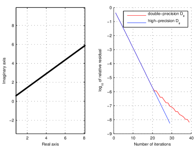
  Fig. 1: Example 1

  

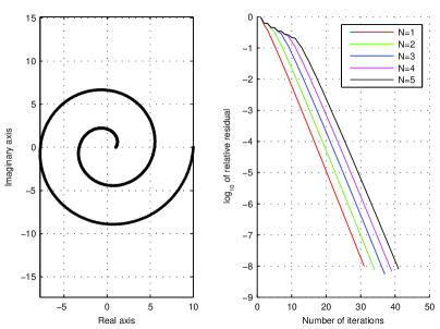
  Fig. 2: Example 2. The diagonal of ${D_{\scriptscriptstyle\#}}$ in the case $N=2$ is plotted on the left panel.

• Example 2. Here we computed using five different sets of angles. We chose $\phi_{1}^{(N)}=0,\phi_{n}^{(N)}=N$, where $N=1,\dots,5$, and the rest of $\phi_{j}^{(N)}$ were linearly interpolated between the extremes. See Figure 2.

  

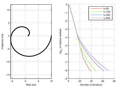
  Fig. 3: Example 3

  

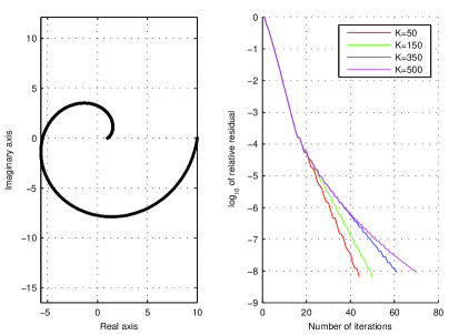
  Fig. 4: Example 4

• Example 3. Let $\widetilde{\phi}_{1}=0,\widetilde{\phi}_{n}=1$ and the rest of $\widetilde{\phi}_{j}$ linearly interpolated between the extremes (Example 2 case $N=1$). Additionally, a random vector $\rho\in{\mathbb{C}}^{n}$ was generated with entries uniformly distributed between $0$ and $10^{-10}$. Given an integer $k$ such that $1\leq k\leq n$, we chose four different sets of angles in (27) by $\phi_{j}^{(k)}=\widetilde{\phi}_{j}+\rho_{j}$ for $j\leq k$ and $\phi_{j}^{(k)}=\widetilde{\phi}_{j}$ for $j>k$. The results are displayed in Figure 3.

• Example 4. Let $\widetilde{\phi}_{j}$ and $\rho$ be as in Example 3. Given an integer $K$ such that $1\leq K\leq n$, we now chose four different sets of angles in (27) by $\phi_{j}^{(K)}=\widetilde{\phi}_{j}$ for $j\leq n-K$ and $\phi_{j}^{(k)}=\widetilde{\phi}_{j}+\rho_{j}$ for $j>n-K$. The results are displayed in Figure 4.

• Example 5. We chose two different sets of angles. For the first set, $\phi_{j}^{(1)}$ was chosen uniformly distributed between $0$ and $1$. For the second set, we chose $\phi_{1}^{(2)}=0,\phi_{n}^{(2)}=1$ and for every odd $j$ the angle $\phi_{j}^{(2)}$ is linearly interpolated between the extremes. For even $j$ we linearly interpolated $\phi_{j}^{(2)}$ between $0$ and $2$. The results in Figure 5 show that the residual makes almost no progress at every other iteration step. The residual for the second set of angles closely follows, but makes more even progress at all iteration steps.

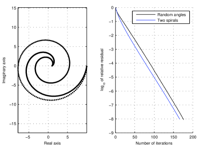
Fig. 5: Example 5. Only the diagonal of ${D_{\scriptscriptstyle\#}}$ in the two spirals case is plotted on the left panel.

References

- [1] G.W. Anderson, A. Guionnet, O. Zeitouni, An Introduction to Random Matrices, Cambridge University Press, New York, 2010.
- [2] K. Astala, J. Mueller, A. Perämäki, L. Päivärinta and S. Siltanen, Direct electrical impedance tomography for nonsmooth conductivities, Inverse Probl. Imaging., 5 (2011), pp. 531–549.
- [3] M.B. Balk, Polyanalytic Functions, Wiley/VCH, Weinh., 1991.
- [4] B. Beckermann, Complex Jacobi matrices, J. Comp. Appl. Math., 127 (2001), pp. 17–65.
- [5] A. Bunse-Gerstner and R. Stöver, On a conjugate gradient-type method for solving complex symmetric linear systems, Linear Alg. Appl., 287 (1999), pp. 105–123.
- [6] P. Deift, Orthogonal Polynomials and Random Matrices: A Riemann-Hilbert Approach, Vol. 3 Courant Lecture Notes in Mathematics, New York University, Courant Institute of Mathematical Sciences, New York, 1999.
- [7] V. Didenko and B. Silbermann, Approximation of Additive Convolution-Like Operators: Real -Algebra Approach, Birkhäuser, Basel, 2008.
- [8] A. Edelman, The probability that a random real Gaussian matrix has real eigenvalues, related distributions, and the circular law, J. Multivariate Anal., 60 (1997), pp. 203–232.
- [9] T. Eirola, M. Huhtanen and J. von Pfaler, Solution methods for -linear problems in , SIAM J. Matrix Anal. Appl., 25 (2004), pp. 804–828.
- [10] G. Forsythe, Generation and use of orthogonal polynomials for data-fitting with a digital computer, J. Soc. Indust. Appl. Math., 5 (1957), pp. 74–88.
- [11] R. Freund, Conjugate gradient-type methods for linear systems with complex symmetric coefficient matrices, SIAM J. Sci. Stat. Comput., 13 (1992), pp. 425–448.
- [12] S.R. Garcia and M. Putinar, Complex symmetric operators and applications, Trans. Amer. Math. Soc., 358 (2006), pp.1285–1315.
- [13] W. Gautschi, Orthogonal polynomials: applications and computation, Acta numerica, 1996, Acta Numer., 5, Cambridge Univ. Press, Cambridge, (1996), pp. 45–119.
- [14] G.H. Golub and C.F. van Loan, Matrix Computations, The Johns Hopkins University Press, the rd ed., 1996.
- [15] G.H. Golub and G. Meurant, Matrices, Moments and Quadrature with Applications, Princeton University Press, Princeton and Oxford, 2010.
- [16] A.Greenbaum and L. Gurvits, Max-min properties of matrix factor norms, SIAM J. Sci. Comput., 15 (1994), pp. 348–358.
- [17] R.A. Horn and C.R. Johnson, Matrix Analysis, Cambridge Univ. Press, Cambridge, 1987.
- [18] M. Huhtanen, Orthogonal polyanalytic polynomials and normal matrices, Math. Comp., 72 (2003), pp. 355–373.
- [19] M. Huhtanen and R. M. Larsen, Exclusion and inclusion regions for the eigenvalues of a normal matrix, SIAM J. Matrix. Anal. Appl., 23 (2002), pp. 1070–1091.
- [20] M. Huhtanen and J. von Pfaler, The real linear eigenvalue problem in , Linear Alg. Appl., 394 (2005), pp. 169–199.
- [21] M. Huhtanen and A. Perämäki, Numerical solution of the -linear Beltrami equation, Math. Comp., 81 (2012), pp. 387–397.
- [22] M. Huhtanen and S. Ruotsalainen, Real linear operator theory and its applications, Integral Equat. Oper. Theory., 69 (2011), pp. 113–132.
- [23] M.G. Kamalvand and Kh.D. Ikramov, A method of congruent type for linear systems with conjugate-normal coefficient matrices, Comp. Math. Math. Phys., 49 (2009), pp. 211–224.
- [24] D. Khavinson and G. Neumann, From the fundamental theorem of algebra to astrophysics: a ”harmonious” path, Notices Amer. Math. Soc., 55 (2008), pp. 666–675.
- [25] M.L. Mehta, Random Matrices, 3rd Ed., Elsevier, Amsterdam, 2004.
- [26] C. Paige and M. Saunders, Solution of sparse indefinite systems of linear equations, SIAM J. Numer. Anal., 12 (1975), pp. 617–629.
- [27] B. Parlett, The Symmetric Eigenvalue Problem, Classics in Applied Mathematics 20, SIAM, Philadelphia, 1997.
- [28] L. Reichel, G.S. Ammar and W.B. Gragg, Discrete least squares approximation by trigonometric polynomials, Math. Comp., 57 (1991), pp. 273–289.
- [29] Y. Saad and M.H. Schultz, GMRES: A generalized minimum residual algorithm for solving nonsymmetric linear systems, SIAM J. Sci. Statist. Comp., 7 (1986), pp. 585–869.
- [30] B. Simon, CMV matrices: Five years after, J. Comp. Appl. Math., 208 (2007), pp. 120–154.
- [31] B. Simon, Szegö’s Theorem and Its Descendants: Spectral Theory for Perturbations of Orthogonal Polynomials, Princeton University Press, Princeton and Oxford, 2010.
- [32] G. Szegö, Orthogonal Polynomials, Colloquium Publications, XXIII, AMS, Providence, 1939.