Chaos synchronization in networks of delay-coupled lasers: Role of the coupling phases

Abstract

We derive rigorous conditions for the synchronization of all-optically coupled lasers. In particular, we elucidate the role of the optical coupling phases for synchronizability by systematically discussing all possible network motifs containing two lasers with delayed coupling and feedback. Hereby we explain previous experimental findings. Further, we study larger networks and elaborate optimal conditions for chaos synchronization. We show that the relative phases between lasers can be used to optimize the effective coupling matrix.

1 Introduction

Coupled nonlinear system may exhibit a remarkable phenomenon called chaos synchronization [1, 2]. The individual systems synchronize to a common chaotic trajectory. This phenomenon has received much attention, due to its potential applications in secure communication [3, 4]. For technological applications semi-conductor lasers are promising systems to implement secure communication schemes using chaos synchronization, because they exhibit fast dynamics, they are cheap and one could utilize the existing telecommunication infrastructure for these lasers [5].

However, due to the fast dynamics of the lasers, propagation distances of already a few meters introduce non-negligible delay times in the coupling. The synchronization of delay-coupled systems in general [6, 7, 8, 9] and in particular delay-coupled lasers [10, 11, 12, 13, 14, 15, 16, 17, 18] has thus been a focus of research in nonlinear dynamics during the last decades.

When the lasers are coupled all-optically, not only delay effects are important, but also the optical coupling phases of the coherently coupled electric fields play an important role. Coherent coupling may result in constructive or destructive interference of incoming signals. When the lasers are synchronized, this interference can occur even if the coupling distance is much larger than the coherence length of the beams [19].

It has been demonstrated experimentally and numerically that by tuning coupling phases one can adjust the level of synchronization ranging from perfect synchronization to almost no correlation [20]. However, the impact of these coupling phases and the resulting interference conditions have so far not been thoroughly investigated.

In this work we derive and discuss synchronization conditions for all-optically coupled lasers. These conditions ensure the existence and stability of a completely synchronized solution, i.e., perfect synchronization of identical lasers. We confirm the analytical results by numerical simulations. For our stability analysis we employ recent results concerning the master stability function (MSF) [21] in the limit of large delay times [22, 23].

The paper is organized as follows. In Sec. 2 we briefly review previous results about synchronization in delay-coupled networks in a general context. These general results are then applied to all-optically coupled lasers. In particular, we discuss the case of two all-optically coupled lasers in detail in Sec. 3. Here, we consider different coupling schemes (unidirectional and bidirectional, open- and closed-loop) and derive the corresponding synchronization conditions. We then discuss synchronization in larger laser networks in Sec. 4 focusing on an experimentally feasible setup. Finally, we conclude with Sec. 5.

2 Synchronization of delay-coupled systems

Consider a delay-coupled network of $N$ identical units

$$\dot{x}_{k}(t)=f(x_{k}(t))+\sum_{j=1}^{N}G_{kj}\,h(x_{j}(t-\tau))\;,$$ (1)

where $x_{k}\in\mathbb{R}^{n}$ is the state vector of the $k$-th node ($k=1,\dots,N$). Here, $f$ is a function describing the local dynamics of an isolated node, $G_{kj}$ is a coupling matrix that determines the coupling topology and the strength of each link in the network, $h$ is a coupling function, and $\tau$ is the delay time in the connection, which is assumed to be equal for all links. A necessary condition for perfect synchronization is that the matrix $G$ has a constant row sum

$${\bf C1:}\qquad\sigma=\sum_{j=1}^{N}G_{kj}\;,$$ (2)

independent of $k$. This condition ensures that an invariant synchronization manifold exists. Note that in this case the row sum $\sigma$ is an eigenvalue of the matrix $G$ corresponding to the eigenvector $(1,1,\dots,1)$ of synchronized dynamics. For a given constant row sum $\sigma$ the dynamics in the synchronization manifold of Eq. (1) is

$$\dot{\bar{x}}(t)=f[\bar{x}(t)]+\sigma h[\bar{x}(t-\tau)]\;.$$ (3)

where $\bar{x}(t)=x_{1}(t)=x_{1}(t)=\dots=x_{N}(t)$ denotes the synchronized solution.

Note that condition C1 addresses mathematically perfect synchronization. For realistic systems it is important to investigate what happens to the synchronization manifold under small perturbations of the perfect setup, such as parameter mismatch of the individual elements or coupling strength mismatch leading to a slightly broken condition C1. On one hand, there has been some recent progress in addressing parameter mismatch within the MSF framework [24, 25] and it might be interesting to apply these new methods to the laser system. On the other hand, slight perturbations of the perfect setup are also related to the question whether the synchronization manifold is normally hyperbolic [26]. Although these questions are important for realistic systems, we will focus our analytic investigations on the case of perfect synchronization to highlight our main message: the importance of the coupling phases.

As we will discuss below, the necessary condition C1 becomes quite involved for the case of optically coupled lasers, because here the matrix $G$ is complex valued due to optical phase factors in the coupling and, additionally, the lasers can have relative phase shifts, which effectively allow the system to adjust the coupling matrix to some extent.

If condition C1 is satisfied and a synchronization manifold exists, the stability problem of the synchronized solution can be approached using the MSF [21]. The MSF depends on a complex parameter $re^{i\psi}$ and is defined as the largest Lyapunov exponent $\lambda(re^{i\psi})$ arising from the variational equation

$$\dot{\xi}(t)=Df[\bar{x}(t)]\,\xi(t)+re^{i\psi}Dh[\bar{x}(t-\tau)]\,\xi(t-\tau)\;,$$ (4)

where $\bar{x}(t)$ is the synchronized trajectory of the system determined by Eq. (3) and $Df$ and $Dh$ are Jacobians.

The synchronized state is stable for a given coupling topology if the MSF is negative at all transversal eigenvalues $\gamma_{k}$ of the coupling matrix ($\lambda(\gamma_{k})<0$). Here, transversal eigenvalue refers to all eigenvalues except for the eigenvalue $\sigma$ associated to perturbations within the synchronization manifold with corresponding eigenvector $(1,\,1,\,\dots,\,1)$.

The dynamical time scale of a semiconductor laser is given by the relaxation oscillation period $T_{RO}$. Typical values of $T_{RO}$ for semiconductor lasers are between $10^{-10}\textrm{s}$ and $10^{-9}\textrm{s}$. This time scale corresponds to about $3\textrm{cm}$ – $30\textrm{cm}$ of optical path-length in air. The coupling distances between the lasers is usually of the order of meters or even much larger [5]. In this case the coupling delay time is much larger than the intrinsic time scale $\tau\gg T_{RO}$ of the lasers. The case of large delay times is an import limit for delayed systems [27, 28, 29, 30, 31, 32].

We recently showed [22] that in any network the stability problem for the synchronized state is drastically simplified in this limit of large delay times:

• The MSF is rotationally symmetric around the origin in the complex plane, i.e., $\lambda(r\,e^{i\psi})$ is independent of $\psi$.

• If $\lambda(0)>0$, then $\lambda(re^{i\psi})=\lambda(0)$ for all $r$ (and $\psi$).

• If $\lambda(0)<0$, then the MSF is monotonically growing with respect to the parameter $r$ and there is a critical radius $r_{0}$, where it changes sign ($\lambda(r_{0})=0$).

Recently, this structure of the MSF has been been confirmed experimentally [33] and even utilized to predict synchronizability of a network from a simpler motif [33, 34].

Note that the two cases $\lambda(0)>0$ and $\lambda(0)<0$ have recently been discussed in more detail [23]. The case $\lambda(0)<0$ is called weak chaos, since in this case the maximum Lyapunov exponent scales as $\sim 1/\tau$ for $\tau\to\infty$. The case $\lambda(0)>0$, on the other hand, is called strong chaos since the maximum Lyapunov exponent scales as $\mathcal{O}(1)$ for $\tau\to\infty$. It has been shown that for large delay networks can only exhibit chaos synchronization in the regime of weak chaos [22, 23].

The structure of the MSF allows us to draw general conclusions about the synchronizability of a given network topology. In particular, chaos synchronization can only be stable if $\sigma$ is the eigenvalue of $G$ with largest magnitude, i.e., the transversal eigenvalues $\gamma_{1},\,\gamma_{2},\,\dots\gamma_{N-1}$ have smaller magnitude

$${\bf C2:}\qquad|\gamma_{n}|<|\sigma|\;.$$ (5)

This condition (C2) is necessary for chaos synchronization ($|\sigma|>r_{0}$) and it is sufficient for synchronization on a periodic orbit ($|\sigma|<r_{0}$) [22]. In fact the smaller the magnitude of the transversal eigenvalues, the easier it is to synchronize the system.

For given synchronized dynamics (Eq. (3)), i.e., given system parameters and row sum $\sigma$, one can calculate numerically the critical radius $r_{0}$, which then provides a necessary and sufficient condition (C3) for synchronization (provided C1 is fulfilled)

$${\bf C3:}\qquad|\gamma_{n}|<r_{0}\;.$$ (6)

While condition C3 is necessary and sufficient, its disadvantage is that one needs to calculate $r_{0}$ explicitly for the particular synchronized dynamics. In contrast, condition C2 is only necessary for chaotic synchronization, however, its strengths lies in the fact that it depends solely on the coupling topology, i.e, the eigenvalues of $G$, and not on the particular dynamics of the system.

The aim of this paper is to apply the synchronization conditions C1–C3 to a system of two delay-coupled lasers and to laser networks and discuss the consequences for chaos synchronization. In particular, we show how condition C1 gives complicated conditions for the coupling phases of the lasers.

3 Two Lasers

Figure 1: Schematic coupling scheme of two delay-coupled lasers with delayed self-feedback. Each connection has a coupling strengths $\kappa_{kj}$ and a coupling phase $\phi_{kj}$. We consider the case when all delay times are equal.

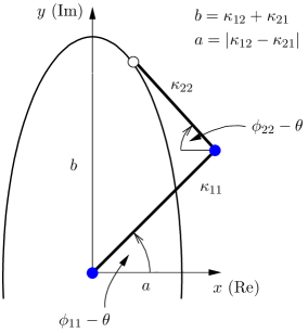
In this section we consider two semiconductor lasers that are delay-coupled to each other with a coupling delay and additionally receive self-feedback with the same delay time $\tau$. The basic coupling scheme is depicted in Fig. 1. The coupled system is described by dimensionless rate equations of Lang-Kobayashi type

$$\dot{E}_{1} ={\textstyle\frac{1}{2}}(1+i\alpha)\left[G(n_{1},\,E_{1})-1\right]E_{1}$$

$$\qquad+\kappa_{11}e^{i\phi_{11}}E_{1}(t-\tau)+\kappa_{12}e^{i\phi_{12}}E_{2}(t-\tau)\;,$$

$$\dot{E}_{2} ={\textstyle\frac{1}{2}}(1+i\alpha)\left[G(n_{2},\,E_{2})-1\right]E_{2}$$

$$\qquad+\kappa_{22}e^{i\phi_{22}}E_{2}(t-\tau)+\kappa_{21}e^{i\phi_{21}}E_{1}(t-\tau)\;,$$

$$T\dot{n}_{1} =p-n_{1}-G(n_{1},\,E_{1})|E_{1}|^{2}\;,$$

$$T\dot{n}_{2} =p-n_{2}-G(n_{2},\,E_{2})|E_{2}|^{2}\;,$$ (7)

where $E_{k}$ and $n_{k}$ are the normalized complex electric field amplitude and the rescaled inversion of the $k$-th laser, respectively, and $\alpha$ is the linewidth enhancement factor, $p$ is the normalized pump current in excess of the threshold, and $\kappa_{ij},\phi_{ij}$ are the coupling amplitudes and phases, respectively, as shown in Fig.. 1. The gain is modeled by

$$G(n,\,E)=\frac{n+1}{1+\mu|E|^{2}}$$ (8)

that takes into account gain saturation effects. Throughout this paper we choose the following model parameters for our numerical simulations, unless stated otherwise: Ratio between carrier and photon lifetime $T=1000$, $p=0.1$, $\alpha=4$, gain saturation $\mu=0.26$.

The optical coupling phases $\phi_{ij}$ are determined by the optical path lengths of the feedback and coupling sections on a subwavelength scale

$$\phi_{ij}=\Omega_{0}\tau_{ij}\;,$$ (9)

where $\Omega_{0}$ is the optical frequency of the laser. Since $\Omega_{0}$ is large, one can for large delay consider the phases as parameters independent of the coupling delays. We thus choose all delays equal, but consider the phases as free parameters.

One important peculiarity of coupled lasers is that the lasers may synchronize with a relative phase shift $u$

$$E_{1}(t)=e^{iu}E_{2}(t)\;.$$

To explicitly treat this relative phase shift, we transform to the new variable $\tilde{E}_{2}$ as

$$\tilde{E}_{2}(t)=e^{iu}E_{2}(t)\;.$$ (10)

After substituting this into Eqs. (7) and omitting the tildas for simplicity we arrive at the following rate equations for the fields

$$\dot{E}_{1} =\dots\quad+\quad\kappa_{11}e^{i\phi_{11}}E_{1}(t-\tau)+\kappa_{12}e^{i(\phi_{12}-u)}E_{2}(t-\tau)\;,$$

$$\dot{E}_{2} =\dots\quad+\quad\kappa_{22}e^{i\phi_{22}}E_{2}(t-\tau)+\kappa_{21}e^{i(\phi_{21}+u)}E_{1}(t-\tau)\;.$$ (11)

The artificially introduced parameter $u$ helps in the analysis of synchronization, because we can discuss existence and stability of the synchronized solution $E_{1}(t)=E_{2}(t)$ in dependence on $u$, thereby treating synchronization of the lasers with a phase shift.

Bringing Eq. (11) into the form of Eq. (1) essentially yields the coupling matrix

$$G=\left[\begin{array}[]{ll}\kappa_{11}e^{i\phi_{11}}&\kappa_{12}e^{i(\phi_{12}-u)}\\ \kappa_{21}e^{i(\phi_{21}+u)}&\kappa_{22}e^{i\phi_{22}}\end{array}\right]\;.$$ (12)

The row sum condition C1 is then given by

$$\kappa_{11}e^{i\phi_{11}}+\kappa_{12}e^{i(\phi_{12}-u)}=\kappa_{22}e^{i\phi_{22}}+\kappa_{21}e^{i(\phi_{21}+u)}\;.$$ (13)

Equation (13) can be interpreted as follows: If for a given set of coupling strengths and coupling phases there exists a phase shift $u$, such that Eq. (13) is fulfilled, then there exists an invariant synchronization manifold. The lasers can thus tune their relative phase shifts appropriately. The stability of the synchronized solution then determines whether synchronization will be observable or not.

As a starting point for the stability analysis we consider the MSF for a laser network with row sum $\sigma$. Since we focus on the large delay case ($\tau=1000\gg T_{RO}$) the rotational symmetry discussed above holds and the MSF $\lambda(re^{i\psi})$ depends solely on $r$.

Figure 2: MSF $\lambda(r)$ in the $(\sigma,\,r)$-plane for $p=0.1$ (panel (a)) and $p=1.0$ (panel (b)). The solid line depicts the critical radius $r_{0}$ with $\lambda(r_{0})=0$. The dotted line is the diagonal line $r=\sigma$. The blue dot corresponds to a parameter set that we will use in the following numerical investigations.

Figure 2 depicts the MSF in the $(\sigma,\,r)$-plane for two different values of the pump current $p=0.1$ (panel (a)) and $p=1$ (panel (b)). When the critical radius $r_{0}$ (solid line) lies below the diagonal line $r=\sigma$ (dotted line), the synchronized solution is chaotic for a network with this row sum, since $\lambda(\sigma)>\lambda(r_{0})=0$. When $r_{0}=\sigma$, as occurs for instance in panel (b) for small values of $\sigma$, the synchronized dynamics is periodic. In this case the solution $\lambda=0$ corresponds to the Goldstone mode of the periodic orbit.

In the following we will consider different coupling topologies of the two lasers. Figure 3 depicts all possible network motifs (up to exchange of $1\leftrightarrow 2$) with more than one connection. The motifs on the left (a-d) can exhibit chaos synchronization in the limit of large delays, while those on the right (e-g) cannot [22] (trivially for motif (g)).

Figure 3: Possible motifs for two delay-coupled lasers. Motifs a)-d) can (for certain parameters) exhibit zero-lag chaos synchronization and are discussed in more detail below. The motifs e)-g) cannot exhibit zero-lag chaos synchronization.

We will now discuss the implications of the synchronization conditions C1–C3 for these motifs and compare the predictions with numerical simulations. We study two measures for synchronization. The first measure is the correlation coefficient of the laser intensities $I_{1},I_{2}$

$$\rho=\frac{\Bigl{\langle}(I_{1}-\langle I_{1}\rangle)\,(I_{2}-\langle I_{2}\rangle)\Bigr{\rangle}}{\sqrt{(\Delta I_{1})^{2}(\Delta I_{2})^{2}}}\;,$$ (14)

where $\langle\cdot\rangle$ denotes the time average and $(\Delta I_{k})^{2}$ denotes the variance of the respective intensity. Although, the correlation coefficient can in principle distinguish between identical synchronization ($\rho=1$) and imperfect (generalized) correlation ($\rho<1$), it is not the most sensitive measure for this purpose, because imperfect synchronization may still yield very large correlation $\rho\approx 1$.

To overcome this disadvantage of the correlation coefficient, we calculate the synchronization probability $P_{S}$. We define $P_{S}$ as the probability that at any time $t$ the relative error between $I_{1}(t)$ and $I_{2}(t)$ is smaller than a threshold $\varepsilon$

$$P_{S}=\mathrm{Prob}\left(\frac{|I_{1}(t)-I_{2}(t)|}{\langle I_{1}\rangle+\langle I_{2}\rangle}<\varepsilon\right)\;.$$ (15)

We choose $\varepsilon=0.01$ in the following.

3.1 Motif (a)

This case is the classical master slave configuration for chaos communication with lasers. It is also referred to as open-loop master slave configuration [35], since the receiver (2) has no self-feedback. The coupling matrix Eq. (12) is in this case given by

$$G=\left[\begin{array}[]{ll}\kappa_{11}e^{i\phi_{11}}&0\\ \kappa_{21}e^{i(\phi_{21}+u)}&0\end{array}\right]\;.$$

The row sum condition C1 then becomes

$$\kappa_{11}e^{i\phi_{11}}=\kappa_{21}e^{i(\phi_{21}+u)}\;.$$

This condition is satisfied if and only if $\kappa_{11}=\kappa_{21}$. The phase shift $u$ can then compensate any choice of coupling phases $\phi_{11}$ and $\phi_{21}$. The second eigenvalue of the coupling matrix is zero, such that the motif is optimal for chaos synchronization and condition C2 is always fulfilled. Whether the systems will synchronize or not then depends on whether $\lambda(0)$ is smaller or larger than zero, i.e., whether the MSF in Fig. 2 is negative (weak chaos) or positive (strong chaos) for $r=0$.

Note that since the coupling is unidirectional, the synchronization properties do not depend on the coupling delay. In particular, if the coupling delay is smaller than the self-feedback delay, anticipated synchronization [36] can be observed [37].

3.2 Motif (b)

This setup consists of two unidirectionally coupled lasers with self-feedback and has been studied in different contexts. The importance of the coupling phases in this coupling scheme has been recognized in [20]. In this reference it was observed in an experiment that depending on the (relative) feedback phases the synchronization behavior ranges from perfect synchronization to an almost uncorrelated state. So far these experiments have not been sufficiently explained. It turns out that the experimental results can be well understood in the light of the synchronization conditions C1–C3:

The coupling matrix corresponding to motif (b) is given by

$$G=\left[\begin{array}[]{ll}\kappa_{11}e^{i\phi_{11}}&0\\ \kappa_{21}e^{i(\phi_{21}+u)}&\kappa_{22}e^{i\phi_{22}}\end{array}\right]$$ (16)

and the row sum condition C1 reads

$$\kappa_{11}e^{i\phi_{11}}=\kappa_{21}e^{i(\phi_{21}+u)}+\kappa_{22}e^{i\phi_{22}}\;.$$

Eliminating $u$, yields the following condition on the coupling strengths and phases

$$\kappa_{21}=\left|\kappa_{11}-\kappa_{22}e^{i\Phi_{\rm rel}}\right|=\sqrt{\kappa_{11}^{2}+\kappa_{22}^{2}-2\kappa_{11}\kappa_{22}\cos(\Phi_{\rm rel})}$$ (17)

with $\Phi_{\rm rel}=\phi_{22}-\phi_{11}$. The phase shift $u$ between the laser fields is then given by

$$u=\phi_{11}-\phi_{21}+\mathrm{Arg}\left(\kappa_{11}-\kappa_{22}e^{i\Phi_{\rm rel}}\right)\;,$$ (18)

where $\mathrm{Arg}$ denotes the complex argument.

Condition C2 on the other hand reads for this case

$$\kappa_{22}<\kappa_{11}=|\sigma|\;,$$

i.e., chaos synchronization is possible, if the self-coupling of laser 2 is weaker than that of laser 1. For a given set of parameters, synchronization is stable if condition C3 is fulfilled, i.e., if

$$\kappa_{22}<r_{0}(\kappa_{11})\;.$$ (19)

To illustrate these conditions, we consider the following parameter set

$$\kappa_{11}=0.2,\quad\kappa_{22}=0.09,\qquad\phi_{11}=0,\qquad\phi_{21}=0$$ (20)

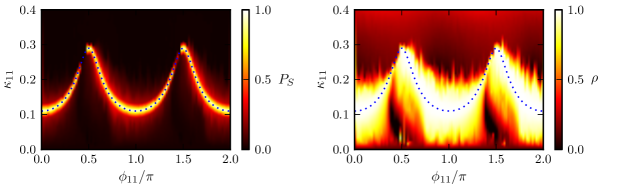
and vary $\Phi_{\rm rel}=\phi_{22}$ and $\kappa_{21}$. These coupling strengths $(\sigma,\,r)=(\kappa_{11},\,\kappa_{22})$ are marked by a blue dot in Fig. 2a and are chosen such that synchronization is stable (condition C3 is fulfilled).

Figure 4: (Motif (b)) Synchronization probability $P_{S}$ (left) and correlation coefficient $\rho$ (right) as a function of $\phi_{22}=\Phi_{\rm rel}$ and $\kappa_{21}$. The dotted line corresponds to the synchronization condition C1 (Eq. (17)). Other parameters: $\kappa_{11}=0.2$, $\kappa_{22}=0.09$, $\phi_{11}=\phi_{21}=0$.

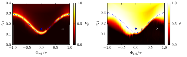
Figure 4 depicts the correlation coefficient $\rho$ and the synchronization probability $P_{S}$ in the $(\Phi_{\rm rel},\,\kappa_{21})$-plane. The dotted line corresponds to Eq. (17), where condition C1 is satisfied. This condition clearly coincides with high synchronization probabilities.

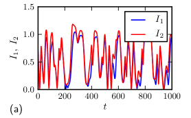
As discussed above, high correlations are also possible without perfect synchronization. In the regions of high correlation and low synchronization probabilities, we observe generalized synchronization. Figure 5(a) shows an example intensity time series observed in these regions. The parameters correspond to the blue dot in Fig 4.

Figure 5: Panel (a): Generalized synchronization for $\kappa_{21}=0.15$ $\phi_{22}=\Phi_{\rm rel}=0$ (blue dot in Fig. 4). Panel (b): No synchronization for $\kappa_{21}=0.15$ $\phi_{22}=\Phi_{\rm rel}=\frac{3}{4}\pi$ (white cross in Fig. 4). Other parameters as in Fig. 4.

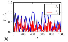
The blue dotted line (condition C1) in Fig 4 roughly marks the boundary between regions of high and low correlations. Below the line, we observe no synchronization at all. An examplary time series in this regime (corresponding to the white cross in Fig. 4) is shown in Fig. 5(b). The correlation in this case is very low. Interestingly, the dynamics of the second laser has, in this case, a strong high-frequency component. The occurrence of this high-frequency component can be understood as a result of the non-locking behavior. Since laser 2 does not lock to the signal of laser 1, the overall input signal of laser 2 is given by the interference of two (almost) independent chaotic signals, namely the signal from laser 1 and the self-feedback signal from laser 2. In this interference signal the high-frequency component is present due to a fast alternation of constructive and destructive interference. Indeed, by switching off the coupling ($\kappa_{21}=0$) and calculating the intensity of an interference signal $I_{\rm intf}=|E_{1}(t)+E_{2}(t)|^{2}$ one can already observe the high-frequency component. For non-zero coupling this interference signal drives laser 2, leading to even higher-order effects.

In Fig. 4(left) there is a region on the dotted line $\Phi_{\rm rel}\in[0.2\pi,0.5\pi]$, where the synchronization probability is low. In this region we observe multistability between identical synchronization solution, a state of generalized synchronization similar to Fig. 5(a), and an uncorrelated state similar to Fig. 5(b). Which state is chosen depends in our deterministic simulations sensitively on the initial conditions. Including noise in the simulation results in spontaneous switching between the three states, albeit it is hard to distinguish between identical synchronization and generalized synchronization in the presence of noise.

Thus although our synchronization condition C1–C3 give the correct existence and stability of the identical synchronized solution, we certainly cannot exclude the existence of other attractors.

The experimental investigations in Ref. [20] were performed under similar parameter conditions, i.e., $\kappa_{22}<\kappa_{11}$ (obeying condition C2). As $\Phi_{\rm rel}$ was varied, the correlation varied from almost perfect to almost no correlation. Varying $\Phi_{\rm rel}$ for a fixed value of $\kappa_{21}$ in Fig. 4 reproduces this behavior, provided the value of $\kappa_{21}$ intersects the dotted synchronization curve. Thus the experimental results can be understood as interference effects, which may or may not lead to the existence of a synchronization manifold, corresponding to high and low correlation, respectively.

3.3 Motif (c)

For this motif the coupling matrix is given by

$$G=\left[\begin{array}[]{ll}\kappa_{11}e^{i\phi_{11}}&\kappa_{12}e^{i(\phi_{12}-u)}\\ \kappa_{21}e^{i(\phi_{21}+u)}&0\\ \end{array}\right]$$ (21)

and the row sum condition C1 reads

$$\kappa_{11}e^{i\phi_{11}}+\kappa_{12}e^{i(\phi_{12}-u)}=\kappa_{21}e^{i(\phi_{21}+u)}\;.$$ (22)

In an experiment with a simple bi-directional coupling, i.e., face-to-face coupling of the lasers, the coupling from laser 1 to laser 2 has the same coupling strengths as the reverse direction:

$$\kappa_{12}\approx\kappa_{21}\;.$$ (23)

We will first consider the more general case, which can be realized in an experiment using optical isolators and separate beam paths for the two coupling directions. We will then consider the natural condition Eq. (23) as a special case.

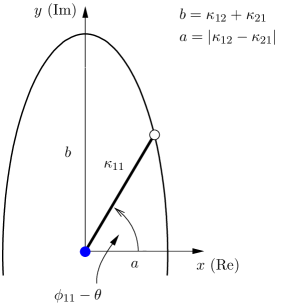
Our aim now is to derive a condition that is equivalent to the existence of a phase shift $u$ satisfying Eq. (22), i.e., we want to eliminate $u$ from the equation. To simplify the discussion, we introduce two parameters:

$$v=u+\frac{\phi_{21}-\phi_{12}}{2},\quad\mbox{and}\quad\theta=\frac{\phi_{21}+\phi_{12}}{2}\;.$$ (24)

Note that $v$ is a “free” parameter, since the phase shift $u$ can be selected by the system. With these parameters Eq. (22) can be written as

$$\kappa_{11}e^{i(\phi_{11}-\theta)}=-\kappa_{12}e^{-iv}+\kappa_{21}e^{iv}\;.$$ (25)

For varying $v$ the terms on the right hand side describe an ellipse in the complex plane with semi-minor axis $a=|\kappa_{12}-\kappa_{21}|$ oriented along the real axis and semi-major axis $b=|\kappa_{12}+\kappa_{21}|$ oriented along the imaginary axis. In order for Eq. (25) to have a solution, the left hand side has to lie on this ellipse. Thus

$$x:=\mathrm{Re}\Bigl{(}\kappa_{11}e^{i(\phi_{11}-\theta)}\Bigr{)}=\kappa_{11}\cos(\phi_{11}-\theta)\;,$$ (26)

$$y:=\mathrm{Im}\Bigl{(}\kappa_{11}e^{i(\phi_{11}-\theta)}\Bigr{)}=\kappa_{11}\sin(\phi_{11}-\theta)$$ (27)

have to obey

$$\frac{x^{2}}{a^{2}}+\frac{y^{2}}{b^{2}}=1\;.$$ (28)

Figure 6: (Motif (c)) Geometric visualization of the synchronization condition (Eq. (25)). If the complex number $\kappa_{11}e^{i(\phi_{11}-\theta)}$ lies on the ellipse, there exists an invariant synchronization manifold.

Figure 7: (Motif (c)) Synchronization probability $P_{S}$ (left) and correlation coefficient $\rho$ (right) as a function of $\phi_{11}$ and $\kappa_{11}$. The dotted line corresponds to the synchronization condition C1 (Eq. (29)). Other parameters: $\kappa_{21}=0.2$, $\kappa_{12}=0.09$, $\phi_{12}=\phi_{21}=0$.

This equation is the desired synchronization condition corresponding to C1. It involves the coupling strengths $\kappa_{11}$, $\kappa_{12}$, and $\kappa_{21}$ and the coupling phases $\phi_{11}$, $\phi_{12}$, and $\phi_{21}$. We can write it as an explicit equation for $\kappa_{11}$

$$\kappa_{11}=\Bigl{[}\frac{\cos^{2}(\phi_{11}-\theta)}{(\kappa_{12}-\kappa_{21})^{2}}+\frac{\sin^{2}(\phi_{11}-\theta)}{(\kappa_{12}+\kappa_{21})^{2}}\Bigr{]}^{-1/2}\;.$$ (29)

Note that for the degenerate case $\kappa_{12}=\kappa_{21}$, i.e., $a=0$, the relevant condition becomes

$$x=0,\qquad\mbox{and}\qquad y^{2}\leq b^{2}\;.$$ (30)

A necessary condition on the coupling strengths for the existence of a solution is

$$|\kappa_{12}-\kappa_{21}|\leq\kappa_{11}\leq\kappa_{12}+\kappa_{21}\;.$$ (31)

To obtain the phase shift $u$, we split Eq. (25) into real and imaginary part and solve for $v$. This yields

$$v=\mathrm{Arg}\left(\frac{x}{\kappa_{21}-\kappa_{12}}+i\,\frac{y}{\kappa_{21}+\kappa_{12}}\right)\;.$$ (32)

The phase shift $u$ is obtained from the definition of $v=u+(\phi_{21}-\phi_{12})/2$.

We now discuss condition C2 and C3, which concern the eigenvalue of $G$ other than the row sum. When $G$ has a constant (complex) row sum $\sigma$, this row sum is an eigenvalue of $G$. Since the determinant of a matrix is the product of its eigenvalues, we have the following equation for the second eigenvalue $\gamma_{1}$ of $G$

$$|\det G|=|\kappa_{12}\kappa_{21}|=|\sigma||\gamma_{1}|\;.$$ (33)

On the other hand, there is only one entry $\kappa_{21}e^{i(\phi_{21}+u)}$ in the second row of $G$ (see Eq. (21)), such that in the case of constant row sum we have

$$|\sigma|=\kappa_{21},\qquad\mbox{and}\qquad|\gamma_{1}|=\kappa_{12}\;.$$ (34)

Thus chaos synchronization is possible if (C2)

$$\kappa_{12}<\kappa_{21}=|\sigma|\;.$$ (35)

For given parameters (given $r_{0}$) synchronization is stable if and only if (C3)

$$\kappa_{12}<r_{0}(\kappa_{21})\;.$$ (36)

Again, we illustrate these conditions by numerical simulations. We choose

$$\kappa_{12}=0.09,\qquad\kappa_{21}=0.2,\qquad\phi_{12}=0,\qquad\phi_{21}=0\;.$$ (37)

The coupling strength again corresponds to the blue dot in Fig. 2a, such that synchronization is stable if a synchronization manifold exists. Similarly to the case of motif (b), there are small regions of low synchronization probability on the dotted curve in Fig. 7(left). These again correspond to regions of multistability and the simulations depend sensitively on initial conditions.

Coming back to the most natural face-to-face coupling (Eq. (23)) with

$$\kappa_{12}=\kappa_{21}$$ (38)

it becomes clear from Eq. (35) that chaos synchronization is not possible in this simple setup. To synchronize the two lasers in this motif one needs an asymmetric coupling.

3.4 Motif (d)

We now consider motif (d), where all possible couplings are present. The corresponding coupling matrix is given by

$$G=\left[\begin{array}[]{ll}\kappa_{11}e^{i\phi_{11}}&\kappa_{12}e^{i(\phi_{12}-u)}\\ \kappa_{21}e^{i(\phi_{21}+u)}&\kappa_{22}e^{i\phi_{22}}\end{array}\right]\;.$$ (39)

The row sum condition C1 is given by

$$\kappa_{11}e^{i\phi_{11}}+\kappa_{12}e^{i(\phi_{12}-u)}=\kappa_{21}e^{i(\phi_{21}+u)}+\kappa_{22}e^{i\phi_{22}}\;.$$ (40)

Below we will discuss this condition in more detail. First, however, we turn to conditions C2 and C3 involving the eigenvalues $\sigma$ (row sum) and $\gamma$ of the matrix $G$.

Assuming that the row sum condition Eq. (40) is satisfied, we solve Eq. (40) for $\kappa_{11}e^{i\phi_{11}}$ and replace this term in the coupling matrix (39). The resulting matrix then has the eigenvalues

$$\sigma =\kappa_{22}e^{i\phi_{22}}+\kappa_{21}e^{i(\phi_{21}+u)}\qquad\mbox{and}$$ (41)

$$\gamma =\kappa_{22}e^{i\phi_{22}}-\kappa_{12}e^{i(\phi_{12}-u)}\;.$$ (42)

The condition C2 ($|\gamma|<|\sigma|$) gives (after some straightforward calculations)

$$\kappa_{12}^{2} -2\kappa_{12}\kappa_{22}\cos(\phi_{12}-\phi_{22}-u)$$ (43)

$$<\kappa_{21}^{2}+2\kappa_{21}\kappa_{22}\cos(\phi_{21}-\phi_{22}+u)\;.$$

The sufficient condition C3 similarly yields

$$\sqrt{\kappa_{12}^{2}-2\kappa_{12}\kappa_{22}\cos(\phi_{12}-\phi_{22}-u)+\kappa_{22}^{2}}<r_{0}(\sigma)\;.$$ (44)

In contrast to the previous cases, it is not possible to eliminate the phase shift $u$ between the lasers directly. We will, however, obtain a formula for $u$ below.

We now further discuss the row sum condition Eq. (40) and aim to eliminate the relative phase shift $u$. The calculation is similar to that done for motif (c), only more involved. Using the same parameters as for the case of motif (c) (Eq. (24))

$$v=u+\frac{\phi_{21}-\phi_{12}}{2},\quad\mbox{and}\quad\theta=\frac{\phi_{21}+\phi_{12}}{2}\;,$$ (45)

we obtain

$$\kappa_{11}e^{i(\phi_{11}-\theta)}-\kappa_{22}e^{i(\phi_{22}-\theta)}=-\kappa_{12}e^{-iv}+\kappa_{21}e^{iv}\;.$$ (46)

Again $v$ is a free parameter, since it is proportional to the relative phase shift $u$, which can be selected by the system. This equation corresponds to the geometric problem visualized in Fig. 8. For varying $v$ the terms on the right hand side describe an ellipse in the complex plane with semi-minor axis $a=|\kappa_{12}-\kappa_{21}|$ oriented along the real axis and semi-major axis $b=\kappa_{12}+\kappa_{21}$ oriented along the imaginary axis. For the equation to have a solution the real and imaginary part of the left hand side have to lie on this ellipse. Thus

$$x :=\kappa_{11}\cos(\phi_{11}-\theta)-\kappa_{22}\cos(\phi_{22}-\theta)$$

$$y :=\kappa_{11}\sin(\phi_{11}-\theta)-\kappa_{22}\sin(\phi_{22}-\theta)$$ (47)

have to obey

$$\frac{x^{2}}{a^{2}}+\frac{y^{2}}{b^{2}}=1\;.$$ (48)

Equation (48) is the final condition, which has to be fulfilled in order for the synchronization manifold to be invariant.

Figure 8: (Motif (d)) Geometric visualization of the synchronization condition (Eq. (46)). If the sum of the two complex numbers $\kappa_{11}e^{i(\phi_{11}-\theta)}$ and $\kappa_{22}e^{i(\phi_{22}-\theta)}$ lies on the ellipse, there exists an invariant synchronization manifold.

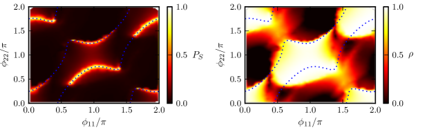
Movie 1 (animation.mpg) illustrates how the geometrical problem of Fig. 8 results in the dotted synchronization curves in Fig. 9.

Figure 9 depicts the correlation coefficient and the synchronization probability in the ($\phi_{11},\,\phi_{22})$-plane for a fixed set of coupling strengths and cross-coupling phases. On the dotted lines the synchronization condition C1 (Eq. (48)) is fulfilled. The lasers exhibit strong synchronization on this curve. For this motif, the row sum $\sigma$ and the transversal eigenvalue $\gamma$ depend on the parameters $\phi_{11}$ and $\phi_{22}$. Due to this dependence, the synchronization condition C3 is not satisfied everywhere on the dotted line and identical synchronization is only stable on parts of the curve. Additionally, we again have the effect of multistability as discussed for the last two motifs, which can result in low synchronization probability on the dotted curve.

Figure 9: (Motif (d)) Synchronization probability $P_{S}$ (left) and correlation coefficient $\rho$ (right) as a function of $\phi_{11}$ and $\phi_{22}$. The dotted line corresponds to the synchronization condition C1 (Eq. (48)). Other parameters: $\kappa_{11}=0.25$, $\kappa_{12}=0.1$, $\kappa_{21}=0.25$, $\kappa_{22}=0.15$, $\phi_{12}=\phi_{21}=0$.

Similarly to the case of motif (c), the relative phase shift $u$ can be found by solving Eq. (46) for $v$

$$v=\mathrm{Arg}\left(\frac{x}{\kappa_{21}-\kappa_{12}}+i\,\frac{y}{\kappa_{21}+\kappa_{12}}\right)\;$$ (49)

and using the definition of $v=u+(\phi_{21}-\phi_{12})/2$. This phase shift can then be used in condition C2 and C3 (Eqs. (43) and (44)).

In order for Eq. (48) to have a solution, the two vectors with respective lengths $\kappa_{11}$ and $\kappa_{22}$ have to be able to reach the ellipse, i. e., the sum of the magnitudes $\kappa_{11}+\kappa_{22}$ has to be larger or equal to the length of the semi-minor axis $a=|\kappa_{12}-\kappa_{21}|$. Similarly, the absolute value of the magnitude difference $|\kappa_{11}-\kappa_{22}|$ has to be smaller or equal to the length of the semi-major axis $b=\kappa_{12}+\kappa_{21}$. We thus obtain two conditions for the existence of a solution

$$(\kappa_{11}+\kappa_{22})^{2} \geq (\kappa_{12}-\kappa_{21})^{2}\;,$$

$$(\kappa_{11}-\kappa_{22})^{2} \leq (\kappa_{12}+\kappa_{21})^{2}\;.$$ (50)

If and only if the coupling strengths fulfill Eqs. (50), there is a combination of phases such that condition (48) is satisfied.

In many optical setups the forward and backward directions have approximately equal coupling strengths $\kappa_{12}\approx\kappa_{21}$. This holds for instance for a setup where the lasers are coupled via a common mirror (see Sec. 4.2) or where the lasers are coupled face-to-face. In this case the ellipse becomes a line along the $y$-axis stretching from $-b$ to $b$. Thus Eq. (48) reduces to $x=0$ with the supplementary condition $y^{2}\leq b^{2}$.

4 Laser networks

We now move from the two-laser system to networks of $N$ all-optically coupled lasers. The synchronization of laser networks is on one hand important for applications for instance in high power laser arrays, where the synchronization of optical phases yields an intensity $I\propto N^{2}$ for interfering beams in contrast to the case of randomly distributed phases that gives $I\propto N$ [38, 39].

On the other hand, laser networks have been proposed as optical information processing systems [40, 41]. Understanding stability properties of dynamical states in these networks is a necessary first step for controlling and utilizing these systems.

For a network of $N$ all-optically coupled lasers, the coupling terms in the Lang-Kobayashi rate equations are given by

$$\dot{E}_{k}=\dots+\sum_{j=1}^{N}\kappa_{kj}\,e^{i\phi_{kj}}E_{j}(t-\tau)\;.$$ (51)

Here $\kappa_{kj}$ and $\phi_{kj}$ are matrices describing the coupling strength and coupling phase, respectively, of the connection $j\rightarrow k$. Again the lasers may synchronize with relative phase shifts $u_{k}$, which we define with respect to laser 1

$$E_{1}(t)=e^{iu_{k}}E_{k}(t)\;,$$ (52)

i.e., $u_{1}=0$. Performing the corresponding transformation (as before in Eq. (11))

$$\tilde{E}_{k}(t)=e^{iu_{k}}E_{k}(t)$$ (53)

and omitting the tildas for simplicity we obtain the field equations

$$\dot{E}_{k}=\dots+\sum_{j=1}^{N}\kappa_{kj}\,e^{i(\phi_{kj}+u_{k}-u_{j})}E_{j}(t-\tau)\;.$$ (54)

The necessary condition C1 for synchronization is then stated as follows: There exists an invariant synchronization manifold if and only if there is a combination of relative phases $u_{k}$ ($k=2,\dots,N$), such that the complex row sum

$$\sigma_{k}=\sum_{j=1}^{N}\kappa_{kj}\,e^{i(\phi_{kj}+u_{k}-u_{j})}$$ (55)

is independent of $k$. As we saw before, this condition is already very difficult to analyze for two lasers when all four connections are present. In an experiment it may be possible to actively control two or three phases accurately using for instance piezo positioning of mirrors, or passive wave-guides where the optical path-lengths can be controlled through an injection current [42]. However, it is virtually impossible to actively control more than a few phases in this way. For larger networks, optoelectronic [43, 44, 45], incoherent optical feedback [46, 47] or coupling via a common relay [13, 16] may thus be a more promising coupling method. However, in certain cases all-optical coupling may be feasible in an experimental situation. We discuss such a feasible setup below.

To illustrate the complexity of the synchronization condition C1 in a simple case, we consider a system of bidirectionally coupled lasers.

4.1 Rings of bi-directionally coupled lasers

For rings of bi-directionally coupled lasers, the coupling matrix has the following principal structure

$$G=\left[\begin{array}[]{ccccc}0&G_{12}&&&G_{1N}\\ G_{21}&0&G_{23}&&\\ &G_{32}&\ddots&\ddots&\\ &&\ddots&\ddots&G_{N-1,N}\\ G_{N1}&&&G_{N,N-1}&0\end{array}\right]\;,$$ (56)

with $G_{kj}=\kappa_{kj}\,e^{i(\phi_{kj}+u_{k}-u_{j})}$. We then obtain the following row sums

$$\sigma_{1} =\kappa_{12}\,e^{i(\phi_{12}+u_{1}-u_{2})}+\kappa_{1N}\,e^{i(\phi_{1N}+u_{1}-u_{N})}\;,$$

$$\sigma_{2} =\kappa_{23}\,e^{i(\phi_{23}+u_{2}-u_{3})}+\kappa_{21}\,e^{i(\phi_{21}+u_{2}-u_{1})}\;,$$

$$\vdots$$

$$\sigma_{N-1} =\kappa_{N-1,N}\,e^{i(\phi_{N-1,N}+u_{N-1}-u_{N})}+\kappa_{N-1,N-2}\,e^{i(\phi_{N-1,N-2}+u_{N-1}-u_{N-2})}\;,$$

$$\sigma_{N} =\kappa_{N,1}\,e^{i(\phi_{N,1}+u_{N}-u_{1})}+\kappa_{N,N-1}\,e^{i(\phi_{N,N-1}+u_{N}-u_{N-1})}\;.$$ (57)

The necessary synchronization condition C1 then corresponds to $2(N-1)$ equations (each complex equation yields two real equations)

$$\sigma_{1}=\sigma_{2},\quad\sigma_{2}=\sigma_{3},\quad\dots\quad\sigma_{N-1}=\sigma_{N}\;.$$ (58)

However, there are only $N-1$ relative phases $u_{j}$ ($u_{1}=0$) that the system can choose freely. Thus, in an experiment we need to control $N-1$ coupling phases to satisfy the synchronization condition C1. For a ring of $N=3$ elements, controlling two coupling phases may still be feasible, but this approach quickly fails for larger $N$.

4.2 Coupling via a common mirror

We will now discuss one promising all-optical setup that should, in principle, be robust to phase mismatches. Consider the setup [40] sketched in Fig. 10. The laser fields are coupled into a common fiber, which is terminated by a mirror. As before, we assume that the coupling delays are equal (the light paths are equally long on a cm scale), but allow for coupling phases, i.e., differences in optical path-lengths on wavelength scales.

Figure 10: Coupling of multiple lasers via a common mirror.

In this setup, the connection from each laser $k$ to the mirror corresponds to a certain optical path length with a corresponding phase $\psi_{k}$. The coupling phase from laser $j$ to laser $k$ is then given by

$$\phi_{kj}=\psi_{k}+\psi_{j}\;.$$ (59)

Similarly, the connection from each laser to the mirror has an associated coupling strength $c_{k}$, which could in an experiment be controlled by an attenuator in the corresponding fiber. The coupling from laser $j$ to laser $k$ then has an effective coupling strength

$$\kappa_{kj}=c_{k}\cdot c_{j}\;.$$ (60)

Under these conditions, the row sum is given by

$$\sigma_{k}=\sum_{j=1}\kappa_{kj}\,e^{i(\phi_{kj}+u_{k}-u_{j})}=c_{k}e^{i(\psi_{k}+u_{k})}\sum_{j=1}^{N}c_{j}\,e^{i(\psi_{j}-u_{j})}\;.$$ (61)

The sum on the right hand side is a complex number independent of $k$. The row sum condition can thus be satisfied if the prefactor is also independent of $k$, i.e., all coupling strengths are equal ($c_{k}=c$) and the relative phases $u_{k}$ are chosen by the system to give

$$\psi_{1}=\psi_{k}+u_{k}\qquad(k=2,\dots,N)\;.$$ (62)

In essence, all lasers couple to the optical mean field and compensate for the difference in optical path length of their individual fiber by adjusting their relative phase shift. As long as the setup obeys Eqs. (59) and (60), the coupling phases $\psi_{k}$ may vary, e.g., due to thermal effects, and do not need to be controlled.

Assuming that all coupling strengths are equal and the relative phases $u_{k}$ are tuned appropriately by the system the coupling matrix is given by

$$G_{kj}=c^{2}\,e^{i(\psi_{k}+\psi_{j}+u_{k}-u_{j})}=c^{2}\,e^{i2\psi_{j}}\;.$$ (63)

This matrix has one eigenvalue corresponding to the row sum

$$\sigma=c^{2}\sum_{j=1}^{N}e^{i2\psi_{j}}$$ (64)

and the $N-1$ transversal eigenvalues are zero

$$\gamma_{n}=0\qquad(n=1,\dots,N-1)\;,$$ (65)

such that this setup is optimal for synchronization.

Recently, this coupling scheme has been proposed for optical information processing using multi-mode lasers [40]. For multi-mode lasers, the same argument as above holds for each mode, such that the setup is, in principle, robust to phase mismatches. However, it may still be difficult to realize the assumptions Eq. (59) and Eq. (60) in an experimental setup.

5 Conclusion and outlook

We have discussed chaos synchronization conditions for all-optically coupled lasers. In all-optical coupling, the coupling phases play a crucial role for the synchronizability. The condition of constant row sum corresponds to specific interference conditions, i.e., the input signals of each laser should interfere in such a way that each laser receives the same input signal, relative to its own phase. This corresponds to the existence of an identical synchronization manifold. Through interference, the phases may compensate for mismatches in the coupling strengths.

Using these interference arguments we have explained experimental findings [20] and discussed necessary and sufficient conditions for synchronization of all network motifs which contain two all-optically coupled lasers.

Further, we have considered synchronization of larger laser networks, and singled out the difficulties that arise in all-optical coupling schemes due to the interference conditions. We predict that a setup of all-to-all coupling via a common mirror may under certain conditions be robust to phase mismatches and thus be optimal with respect to stability of the synchronized chaotic dynamics.

In a broader context, these results might also be relevant for other networks where phase-sensitive couplings play a role, e.g., networks of Stuart-Landau oscillators with complex coupling constants $\sigma=Ke^{i\beta}$ [7]. These are generic models representative for a large class of oscillator networks.

References

- [1] Arkady S. Pikovsky, Michael G. Rosenblum, and J. Kurths. Synchronization, A Universal Concept in Nonlinear Sciences. Cambridge University Press, Cambridge, 2001.
- [2] S. Boccaletti, J. Kurths, G. Osipov, D. L. Valladares, and C. S. Zhou. The synchronization of chaotic systems. Phys. Rep., 366:1–101, 2002.
- [3] K. M. Cuomo and A. V. Oppenheim. Circuit implementation of synchronized chaos with applications to communications. Phys. Rev. Lett., 71(1):65–68, 1993.
- [4] I. Kanter, E. Kopelowitz, and W. Kinzel. Public channel cryptography: chaos synchronization and Hilbert’s tenth problem. Phys. Rev. Lett., 101(8):84102, 2008.
- [5] A. Argyris, D. Syvridis, L. Larger, V. Annovazzi-Lodi, P. Colet, I. Fischer, J. García-Ojalvo, C. R. Mirasso, L. Pesquera, and K. A. Shore. Chaos-based communications at high bit rates using commercial fibre-optic links. Nature, 438:343–346, 2005.
- [6] M. Dhamala, V. K. Jirsa, and M. Ding. Enhancement of neural synchrony by time delay. Phys. Rev. Lett., 92(7):074104, 2004.
- [7] C. U. Choe, T. Dahms, P. Hövel, and E. Schöll. Controlling synchrony by delay coupling in networks: from in-phase to splay and cluster states. Phys. Rev. E, 81(2):025205(R), 2010.
- [8] W. Kinzel, A. Englert, G. Reents, M. Zigzag, and I. Kanter. Synchronization of networks of chaotic units with time-delayed couplings. Phys. Rev. E, 79(5):056207, 2009.
- [9] I. Kanter, M. Zigzag, A. Englert, F. Geissler, and W. Kinzel. Synchronization of unidirectional time delay chaotic networks and the greatest common divisor. Europhys. Lett., 93(6):60003, 2011.
- [10] H. J. Wünsche, S. Bauer, J. Kreissl, O. Ushakov, N. Korneyev, F. Henneberger, E. Wille, H. Erzgräber, M. Peil, W. Elsäßer, and I. Fischer. Synchronization of delay-coupled oscillators: A study of semiconductor lasers. Phys. Rev. Lett., 94:163901, 2005.
- [11] T. W. Carr, I. B. Schwartz, M. Y. Kim, and R. Roy. Delayed-mutual coupling dynamics of lasers: scaling laws and resonances. SIAM J. Appl. Dyn. Syst., 5(4):699–725, 2006.
- [12] H. Erzgräber, B. Krauskopf, and D. Lenstra. Compound laser modes of mutually delay-coupled lasers. SIAM J. Appl. Dyn. Syst., 5(1):30–65, 2006.
- [13] I. Fischer, R. Vicente, J. M. Buldú, M. Peil, C. R. Mirasso, M. C. Torrent, and J. García-Ojalvo. Zero-lag long-range synchronization via dynamical relaying. Phys. Rev. Lett., 97(12):123902, 2006.
- [14] O. D’Huys, R. Vicente, T. Erneux, J. Danckaert, and I. Fischer. Synchronization properties of network motifs: Influence of coupling delay and symmetry. Chaos, 18(3):037116, 2008.
- [15] V. Flunkert, O. D’Huys, J. Danckaert, I. Fischer, and E. Schöll. Bubbling in delay-coupled lasers. Phys. Rev. E, 79:065201 (R), 2009.
- [16] Jordi Zamora-Munt, C. Masoller, Jordi Garcia-Ojalvo, and R. Roy. Crowd synchrony and quorum sensing in delay-coupled lasers. Phys. Rev. Lett., 105(26):264101, 2010.
- [17] K. Hicke, O. D’Huys, V. Flunkert, E. Schöll, J. Danckaert, and I. Fischer. Mismatch and synchronization: Influence of asymmetries in systems of two delay-coupled lasers. Phys. Rev. E, 83:056211, 2011.
- [18] Y. Aviad, I. Reidler, M. Zigzag, M. Rosenbluh, and I. Kanter. Synchronization in small networks of time-delay coupled chaotic diode lasers. Opt. Express, 20(4):4352–4359, 2012.
- [19] Y. Aviad, I. Reidler, W. Kinzel, I. Kanter, and M. Rosenbluh. Phase synchronization in mutually coupled chaotic diode lasers. Phys. Rev. E, 78(2):025204, 2008.
- [20] M. Peil, T. Heil, I. Fischer, and W. Elsäßer. Synchronization of chaotic semiconductor laser systems: A vectorial coupling-dependent scenario. Phys. Rev. Lett., 88(17):174101, 2002.
- [21] L. M. Pecora and T. L. Carroll. Master stability functions for synchronized coupled systems. Phys. Rev. Lett., 80(10):2109–2112, 1998.
- [22] V. Flunkert, S. Yanchuk, T. Dahms, and E. Schöll. Synchronizing distant nodes: a universal classification of networks. Phys. Rev. Lett., 105:254101, 2010.
- [23] S. Heiligenthal, T. Dahms, S. Yanchuk, T. Jüngling, V. Flunkert, I. Kanter, E. Schöll, and W. Kinzel. Strong and weak chaos in nonlinear networks with time-delayed couplings. Phys. Rev. Lett., 107:234102, 2011.
- [24] J. Sun, E. M. Bollt, and T. Nishikawa. Master stability functions for coupled nearly identical dynamical systems. Europhys. Lett., 85(6):60011, 2009.
- [25] F. Sorrentino and M. Porfiri. Analysis of parameter mismatches in the master stability function for network synchronization. EPL, 93(5):50002, 2011.
- [26] L. Kocarev, Ulrich Parlitz, and Reggie Brown. Robust synchronization of chaotic systems. Phys. Rev. E, (4):3716–3720, 2000.
- [27] J. D. Farmer. Chaotic attractors of an infinite-dimensional dynamical system. Physica D, 4:366, 1982.
- [28] G. Giacomelli and A. Politi. Relationship between delayed and spatially extended dynamical systems. Phys. Rev. Lett., 76:2686, 1996.
- [29] B. Mensour and André Longtin. Power spectra and dynamical invariants for delay-differential and difference equations. Physica D, 113:1–25, 1998.
- [30] M. Wolfrum and S. Yanchuk. Eckhaus instability in systems with large delay. Phys. Rev. Lett., 96:220201, 2006.
- [31] S. Yanchuk, M. Wolfrum, P. Hövel, and E. Schöll. Control of unstable steady states by long delay feedback. Phys. Rev. E, 74:026201, 2006.
- [32] S. Yanchuk and P. Perlikowski. Delay and periodicity. Phys. Rev. E, 79(4):046221, 2009.
- [33] L. Illing, Cristian D. Panda, and Lauren Shareshian. Isochronal chaos synchronization of delay-coupled optoelectronic oscillators. Phys. Rev. E, 84:016213, 2011.
- [34] V. Flunkert. Delay-Coupled Complex Systems. Springer Theses. Springer, Heidelberg, 2011.
- [35] R. Vicente, T. Pérez, and C. R. Mirasso. Open-versus closed-loop performance of synchronized chaotic external-cavity semiconductor lasers. IEEE J. Quantum Electron., 38(9):1197–1204, 2002.
- [36] Henning U. Voss. Anticipating chaotic synchronization. Phys. Rev. E, 61(5):5115–5119, 2000.
- [37] C. Masoller. Anticipation in the synchronization of chaotic semiconductor lasers with optical feedback. Phys. Rev. Lett., 86(13):2782–2785, 2001.
- [38] G. Kozyreff, A. G. Vladimirov, and P. Mandel. Global coupling with time delay in an array of semiconductor lasers. Phys. Rev. Lett., 85(18):3809, 2000.
- [39] S. Wieczorek. Stochastic bifurcation in noise-driven lasers and hopf oscillators. Phys. Rev. E, 79(3):036209, 2009.
- [40] A. Amann, A. Pokrovskiy, S. Osborne, and S. O’Brien. Complex networks based on discrete-mode lasers. In International Workshop on Multi-Rate Processes and Hysteresis, Cork 2008, volume 138 of J. Phys.: Conf. Ser., page 012001. IOP Publishing, 2008.
- [41] L. Appeltant, M. C. Soriano, Guy Van der Sande, J. Danckaert, S. Massar, J. Dambre, B. Schrauwen, C. R. Mirasso, and I. Fischer. Information processing using a single dynamical node as complex system. Nat. Commun., 2:468, 2011.
- [42] S. Schikora, P. Hövel, H. J. Wünsche, E. Schöll, and F. Henneberger. All-optical noninvasive control of unstable steady states in a semiconductor laser. Phys. Rev. Lett., 97:213902, 2006.
- [43] Vladimir S. Udaltsov, J. P. Goedgebuer, L. Larger, and William T. Rhodes. Communicating with optical hyperchaos: Information encryption and decryption in delayed nonlinear feedback systems. Phys. Rev. Lett., 86(9):1892–1895, 2001.
- [44] K. E. Callan, L. Illing, Z. Gao, D. J. Gauthier, and E. Schöll. Broadband chaos generated by an opto-electronic oscillator. Phys. Rev. Lett., 104(11):113901, 2010.
- [45] Bhargava Ravoori, Adam B. Cohen, Jie Sun, Adilson E. Motter, Thomas E. Murphy, and R. Roy. Robustness of optimal synchronization in real networks. Phys. Rev. Lett., 107:034102, 2011.
- [46] F. Rogister, A. Locquet, D. Pieroux, M. Sciamanna, O. Deparis, P. Megret, and M. Blondel. Secure communication scheme using chaotic laser diodes subject to incoherent optical feedback and incoherent optical injection. Opt. Lett., 26(19):1486–1488, 2001.
- [47] David W. Sukow, Karen L. Blackburn, Allison R. Spain, Katherine J. Babcock, Jake V. Bennett, and Athanasios Gavrielides. Experimental synchronization of chaos in diode lasers with polarization-rotated feedback and injection. Opt. Lett., 29(20):2393, 2004.