Abstract

We consider the holography of the Abelian Maxwell-Chern-Simons (MCS) system in Lorentzian three-dimensional asymptotically-AdS spacetimes, and discuss a broad class of boundary conditions consistent with conservation of the symplectic structure. As is well-known, the MCS theory contains a massive sector dual to a vector operator in the boundary theory, and a topological sector consisting of flat connections dual to $U(1)$ chiral currents; the boundary conditions we examine include double-trace deformations in these two sectors, as well as a class of boundary conditions that mix the vector operators with the chiral currents. We carefully study the symplectic product of bulk modes and show that almost all such boundary conditions induce instabilities and/or ghost excitations, consistent with violations of unitarity bounds in the dual theory.

1 Introduction

Since the early days of the holographic correspondence [1, 2, 3], $(2+1)$-dimensional gravitational systems have played a central role in testing and exploring the ideas behind the duality. In fact, with the benefit of hindsight, one can see that the work of Brown and Henneaux on the asymptotic symmetries of three-dimensional spacetimes with a negative cosmological constant [4] displayed some basic features of the correspondence as early as a decade before it was proposed. The 3$d$ gravitational systems of interest in the framework of holography are special in that their field theory duals enjoy an infinite-dimensional (local) conformal symmetry; via the powerful techniques of conformal field theory (CFT), one then has a better grasp of the boundary theory structure which is often lacking in higher-dimensional examples. A beautiful example of this fact is the precise connection between the CFT spectrum and retarded Green’s functions, and black hole quasinormal modes in the bulk [5].

The feature that makes the gauge/gravity correspondence outstanding is that it postulates the equivalence between gravitational weakly-coupled degrees of freedom propagating in the bulk spacetime, and strongly-coupled degrees of freedom in a dual quantum field theory in one less dimension (“the boundary”). A pivotal ingredient in the proposal is the dilatation symmetry of the boundary CFT; broadly speaking, using this symmetry one can relate the masses of the bulk fields to the conformal dimensions of operators in the quantum theory on the boundary, as first established in [2]. However, for a given bulk field, the spectrum of conformal dimensions in the dual quantum field theory is not entirely determined by the masses of the fields. This is intimately related to the fact that the boundary conditions that yield well-defined dynamics are not unique. In fact, in the so-called “bottom-up” holography where the bulk theory is phenomenologically devised, the operator content of the possible dual theories is completely specified only after the boundary conditions for bulk fields have been properly chosen.

In the present article, we will focus on the study of the Abelian Maxwell-Chern-Simons (MCS) theory, frequently referred to as “Topologically Massive Electrodynamics” [6, 7], in three-dimensional asymptotically-AdS spacetimes. The emphasis will be on determining a set of “admissible” boundary conditions, in a sense that will be made precise below; this is crucial to the dictionary problem in the context of the AdS/CFT correspondence, as discussed above. One of the motivations to study Chern-Simons terms in the bulk is that these arise naturally in the context of string theory compactifications, and endow the bulk black hole solutions with $U(1)$ charge (see [8, 9], for example). It is worth mentioning, however, that the MCS system plays a central role in condensed matter physics as well, in particular in the study of fermionic systems in two spatial dimensions, where it describes the low-energy effective theory of the Fractional Quantum Hall Effect (FQHE). Furthermore, even in flat space the MCS theory is often said to be holographic, albeit in a different sense from the above: in the topological limit (where the bulk quasiparticles become infinitely massive), the degrees of freedom are effectively localized on the boundary [10]. From a mathematical point of view, this is the well-known correspondence between three-dimensional Chern-Simons gauge theory and a chiral rational CFT [11, 12, 13, 14, 15, 16, 17]. More recently, the latter correspondence has been refined to reconcile the modular transformation properties of the string theory partition function on $AdS_{3}$ and those of the Chern-Simons theory which dominates its infrared dynamics [18], and the potential relevance of these observations for condensed matter physics was also pointed out. This provides yet another motivation to carefully study the holographic dictionary of the full (finite coupling) MCS theory; here we will do so from a bottom-up perspective, in the hope that our results could be useful in the study of other models which might be interesting for applications of holography to condensed matter physics.

Our analysis starts by determining a broad set of boundary conditions under which the bulk theory is expected to have well-posed dynamics. We find it convenient to approach this problem using the covariant phase space formalism, along the lines of [19, 20, 21]. Within this framework, the first requirement on the boundary conditions is that they lead to a conserved symplectic structure (in the sense of timelike evolution). In the context of holography, this condition can be conveniently rephrased as the vanishing of the symplectic flux on the (radial) boundary. Roughly speaking, the bulk gauge field splits into a “massive”, gauge-invariant piece, and the flat connections. Accordingly, the boundary theory operators organize themselves into two sectors: a vector operator dual to the massive part of the connection, and the well-known $U(1)$ chiral currents (which also arise in the pure Chern-Simons theory). We will obtain a variety of boundary conditions that correspond to double-trace deformations from the dual field theory perspective. In particular, we shall note the possibility of coupling the vector operator and the chiral currents via this mechanism. To our knowledge, these “hybrid” boundary conditions intertwining the massive and topological sectors have not been discussed in the literature; their existence was anticipated in [18], however, where the topology of the spacetime manifold was chosen in such a way that the two sectors effectively decouple.

It is worth emphasizing that all of this physics occurs at finite Maxwell coupling. It is often argued in the literature that the Maxwell coupling should be irrelevant in the infrared; this is certainly true from the bulk perspective. However, the Maxwell coupling is not irrelevant in the UV, and so is an important parameter holographically. One also notes in parallel that in condensed matter systems such as quantum Hall, the Maxwell coupling sets the cut-off scale where quasi-particle excitations live, going away only in the topological limit. It seems quite plausible that such excitations will exist in the holographic theory as well, a subject that we will explore elsewhere.

Having obtained the class of boundary conditions that lead to a conserved symplectic structure, one can examine in detail which of these are consistent with unitarity. Our motivation to consider this restriction comes primarily from the existence of the unitarity bound in conformal field theories (see [22, 23], for example), which dictates that the presence of operators whose dimension is “too low” leads to negative norm states (ghosts). Via the holographic correspondence, this fact should manifest in the bulk physics as well, which is the question we address. As first noted in [24, 25], a closely analogous concern arises when considering bulk scalar fields with sufficiently high masses if one imposes boundary conditions that allow the slow-decaying branch to fluctuate. As a result of this choice, the conformal dimension of the dual operator lies below the unitarity bound and one expects the bulk theories to be ill-defined. Recently, these setups were considered in [26], which confirmed that such bulk theories are indeed pathological and that, generically, they suffer from ghosts.

We will address the question of unitarity by studying the dynamics of the MCS system in $AdS_{3}$ in both global and Poincaré coordinates; in particular, we will discuss the resulting spectrum and symplectic products for the various boundary conditions for which the symplectic structure is conserved. Our main result is that the only boundary conditions consistent with unitarity do not mix the massive and topological sectors, and in particular they require to hold fixed the slower fall-off of the massive mode (i.e. they are of Dirichlet type). In short, the class of permissible boundary conditions is severely restricted by unitarity considerations. Interestingly, we will also find additional ghosts in the flat sector whose presence cannot be linked to unitarity bounds in an obvious way. We will also include an analysis of the symmetries we expect to be present in the dual theory as a result of various choices of boundary conditions.

The three-dimensional MCS theory has been previously considered in the context of AdS/CFT. We refer the reader to [18, 9, 8, 27] for work which focuses on the flat (topological) sector of the theory. The massive sector has also received some attention and the holographic dictionary problem has been studied to some extent [28, 29, 30]. Our results agree with the references above as far as the operator content is concerned. The novelty of our analysis lies in the fact that we have considered a wider class of boundary conditions, including “hybrid” boundary conditions that mix the massive and topological sectors, and analyzed their consistency with unitarity in detail. Additional related work includes [31, 32, 33, 34].

This paper is organized as follows. In section 2 we review the MCS system, the solution of the asymptotic equations of motion on asymptotically $AdS_{3}$ backgrounds, and the corresponding conformal dimensions of dual operators. In section 3 we briefly describe the covariant phase space formalism, and use the conservation of the symplectic structure as a criterion to determine a wide class of a priori admissible boundary conditions in the holographic setup. For all the boundary conditions of interest, we construct the appropriate action principles and compute the one-point functions of the dual operators holographically. We also review the notion of symplectic product, which will play a central role in the analysis of unitarity. In section 4 we discuss the spectrum of excitations in the dual field theory for the class of boundary conditions previously found, and discuss the normalizability of the various bulk modes. In section 5 we present the calculation of the symplectic product for the various normalizable modes, focusing on the existence of ghosts; the requirement of unitarity in the dual theory then leads to a restricted class of permissible boundary conditions, which constitutes our main result. We conclude in section 6 with a discussion of our findings, along with possible extensions and applications. Some useful results used in the body of the paper have been collected in the appendices, as well as a brief discussion of the $U(1)$ symmetries in the dual field theory for the different boundary conditions under consideration.

2 The Maxwell-Chern-Simons system

We consider the Maxwell-Chern-Simons (MCS) system in $(2+1)$ spacetime dimensions,

$$I={} -\frac{1}{4q^{2}}\int_{M}d^{3}x\,\sqrt{|g|}F_{\mu\nu}F^{\mu\nu}-\frac{\hat{\alpha}}{4}\int_{M}d^{3}x\,\varepsilon^{\mu\nu\rho}A_{\mu}F_{\nu\rho}\,,$$ (2.1)

where $q^{2}$ is the gauge coupling (with units of $[length^{-1}]$) and $\hat{\alpha}$ is the (dimensionless) Chern-Simons (CS) coupling. Throughout this paper we work in a fixed background in which we neglect the backreaction of the gauge field on the metric, i.e. $G_{N}/q^{2}\to 0$, where $G_{N}$ is the three dimensional gravitational coupling (which has units of $[length]$). Where appropriate, we will occasionally comment on issues of backreaction, and will consider them in a subsequent publication. The background metrics we consider are solutions of the Einstein equations in the presence of a negative cosmological constant $\Lambda=-1/L^{2}$, and the normalization is chosen such that pure $AdS_{3}$ space is a vacuum solution of the decoupled gravitational sector with radius $L$ and scalar curvature $R=-6/L^{2}$. As usual, in a holographic context the action (2.1) must be supplemented by a collection of boundary terms that render the variational problem well defined and remove divergent contributions; these will be fully specified later on in the paper.

The equations of motion that follow from (2.1) are

$$\nabla_{\nu}F^{\nu\mu}+\frac{\alpha}{2L}\epsilon^{\mu\nu\rho}F_{\nu\rho}=0\,,$$ (2.2)

where we have defined the rescaled CS coupling $\alpha$ as

$$\alpha=q^{2}L\hat{\alpha}\,,$$ (2.3)

which is also dimensionless. Without loss of generality, we will assume $\alpha>0$. When taking backreaction on the metric into account, asymptotically AdS solutions exist only for $\alpha<1$, and we will restrict our discussions in the present paper to that range.

In form language, the Maxwell-CS equation (2.2) can be written as

$$d^{\dagger}F=\frac{\alpha}{L}*F$$ (2.4)

where $d^{\dagger}$ is the adjoint exterior derivative, which in our conventions acts on $F$ as $d^{\dagger}F=-*d(*F)=-\nabla_{\mu}F^{\mu}_{\phantom{\mu}\nu}\,dx^{\nu}$. Hence, the equation of motion implies

$$A=A^{(0)}+B\,,$$ (2.5)

where $A^{(0)}$ is a flat connection and we have defined

$$B\equiv-\frac{L}{\alpha}*F\,.$$ (2.6)

We note that $B$ is, by definition, invariant under the $U(1)$ gauge symmetry of the theory. In a later section we will study the consequences of the splitting (2.5) at the level of the symplectic structure and the boundary conditions in a holographic context.

Since $dB=dA=F$, the equation of motion (2.4) becomes a first order equation for $B$:

$$*dB+\frac{\alpha}{L}B=0\,,$$ (2.7)

which is the familiar equation for a massive vector field. In components, this equation reads

$$\epsilon^{\mu\nu\rho}\partial_{\nu}B_{\rho}+\frac{\alpha}{L}B^{\mu}=0\,.$$ (2.8)

Notice also that the definition (2.6) implies a consistency condition:

$$d^{\dagger}B=0\,,$$ (2.9)

i.e. $B$ is a co-closed form ($\nabla^{\mu}B_{\mu}=0$); naturally, this also follows from the equation of motion (2.7). Acting on (2.7) with $*d$ we can write a second-order equation for $B$,

$$0=d^{\dagger}dB+\frac{\alpha^{2}}{L^{2}}B=\Delta B+\frac{\alpha^{2}}{L^{2}}B\,,$$ (2.10)

where $\Delta=d^{\dagger}d+dd^{\dagger}$ is the Laplacian.

2.1 Asymptotic solutions

For the sake of concreteness, we will write the metric of the asymptotically AdS spacetimes we are interested in as

$$ds^{2}\xrightarrow[r\to\infty]{}L^{2}\frac{dr^{2}}{r^{2}}+\frac{r^{2}}{L^{2}}g^{(0)}_{ij}(x)dx^{i}dx^{j}+\ldots$$ (2.11)

Restricting ourselves to flat connections which are finite at the conformal boundary, the asymptotic form of the solution for the gauge field is then of the form

$$A(r,x)\xrightarrow[r\to\infty]{}A^{(0)}(x)+r^{\alpha}\left(B^{(+)}(x)+\mathcal{O}(r^{-2})\right)+r^{-\alpha}\left(B^{(-)}(x)+\mathcal{O}(r^{-2})\right)\,,$$ (2.12)

where $A^{(0)}$ is flat, i.e. $F^{(0)}=dA^{(0)}=0$. Similarly, solving the equations of motion asymptotically one finds that the radial component $B_{r}$ of the gauge-invariant mode is subleading with respect to the $B_{i}$ components, which are moreover constrained by

$$P_{\pm}^{ij}B_{j}^{\left(\mp\right)}=0\,,\qquad\mbox{where }\quad P_{\pm}^{ij}=\frac{1}{2}\left(g^{(0)ij}\pm\epsilon^{ij}\right).$$ (2.13)

We have adopted the convention that $\epsilon^{ij}=-\varepsilon^{ij}/\sqrt{|g^{(0)}|}$, where $\varepsilon^{ij}$ is the two-dimensional Levi-Civita symbol, related to its three-dimensional counterpart by $\varepsilon^{ij}=\varepsilon^{rij}$. Notice that the projectors $P_{\pm}^{ij}$ satisfy the usual properties: $\left(P_{+}P_{-}\right)^{ij}=P_{+}^{ik}g^{(0)}_{kl}P_{-}^{lj}=0$, $\left(P_{\pm}^{2}\right)^{ij}=P_{\pm}^{ik}g^{(0)}_{kl}P_{\pm}^{lj}=P_{\pm}^{ij}\,$.

2.2 Conformal dimensions

Given the asymptotic expansion (2.12) and noting that the pullback to the boundary of the bulk vector field is simply a boundary vector, we conclude that the standard AdS/CFT dictionary relates $B^{(+)}$ and $B^{(-)}$ with vector operators of dimensions $\Delta_{-}=1-\alpha$ and $\Delta_{+}=1+\alpha$, respectively. On the other hand, the components of $A^{(0)}$ have scaling dimension one. As we shall review below, the components of $A^{(0)}$ along the boundary directions correspond to chiral currents that live on the boundary theory, [11, 12, 13, 10, 14, 15, 16, 17]. We note that the lower scaling dimension is positive as long as $\alpha<1$, which implies that we can allow both fall-offs to fluctuate while preserving locally AdS asymptotics if $\alpha<1$. We have verified this statement explicitly by studying the effect of backreaction on a general asymptotically locally AdS metric of the form (2.11).

It should be noted that the operator of dimension $\Delta_{-}$ violates the unitarity bound $\Delta_{V}=1$ for vector operators in two dimensions for all $\alpha>0$ [22, 23], see also [36] for the explicit expression. This suggests that boundary conditions that allow this degree of freedom to fluctuate should yield pathologies in the bulk; in subsequent sections we shall verify that this is indeed the case.

3 Symplectic structure and boundary conditions

In the present section we study the issue of boundary conditions in the holographic description of the MCS system. We find it convenient to work within the covariant phase space formalism, which we will review shortly. The motivation for employing this formalism is two-fold: first, the classification of the allowed boundary conditions is nicely encoded in a simple vanishing-flux condition; and second, it allows us to classify the spectrum of excitations in a clean way. We emphasize however that this decision is just a matter of personal preference, and the results obtained within this framework should indeed be equivalent to the ones arrived at by more familiar, say canonical, methods.

We now proceed to briefly review the covariant phase space techniques; more detailed discussions can be found in [37, 38, 39, 40, 41]. First, we stress that the construction is inherently Lorentzian, so we shall assume that the spacetime is endowed with a Lorentzian metric. Now, the ingredient that lies at the heart of this construction is the identification of the phase space with the space of solutions of the equations of motion which satisfy certain boundary conditions. This is possible since in any well-defined setup the specification of a point in canonical phase-space, i.e. of initial data, completely determines the subsequent evolution of the system. The other main ingredient is an algebraic structure that determines the dynamics once a Hamiltonian function is given, or crudely speaking, something that contains information about the Poisson brackets. This is nothing but the pre-symplectic structure of the theory, $\Omega$, which can be thought of as a (possibly degenerate) two-form in the tangent space of (linearized) solutions. In other words, $\Omega$ maps a pair of tangent vectors in the space of solutions to the real numbers. Given a background solution $\bar{s}$ and two linearized solutions $\delta_{1}s$ and $\delta_{2}s$, we denote the symplectic product of $\delta_{1}s$ with $\delta_{2}s$ by $\Omega(\delta_{1}s,\delta_{2}s;\bar{s})$. Quite conveniently, this object can be constructed algorithmically given a Lagrangian [37], and we will illustrate this below.

From the discussion above, it follows that the pre-symplectic structure must indeed be conserved in order for the identification of the initial data with the space of solutions to be independent of the surface on which the initial data is specified. This conservation condition is what we shall take as a guiding principle to classify the allowed boundary conditions for the MCS system. It is worth emphasizing here that the boundary conditions are in fact a crucial part of the definition of the phase space of a given theory. As pointed out above, the covariant phase space formalism also provides a useful way to classify the spectrum of excitations of the theory. In particular, we mention that in the presence of gauge symmetries the pre-symplectic structure is degenerate, the gauge orbits being precisely its null directions. Thus, we shall refer to any solution of the equations of motion whose symplectic product with an arbitrary solution vanishes as “pure gauge”. Further nomenclature will be discussed in section 3.4.

After taking the quotient by the gauge directions, the symplectic structure has a unique inverse and this corresponds to the Poisson bracket defined for gauge-invariant quantities. As discussed in detail in [38], this relation can be written succinctly as

$$\{\Omega(\delta_{1}s,\cdot;\bar{s}),\Omega(\delta_{2}s,\cdot;\bar{s})\}_{PB}=-\Omega(\delta_{1}s,\delta_{2}s;\bar{s})\,.$$ (3.1)

Here $\Omega(\delta_{1}s,\cdot;\bar{s})$ is to be understood as a linear function in covariant phase space. Then, the fact that the Poisson bracket and $\Omega$ are the inverse of each other follows trivially by writing (3.1) in component notation. Finally, we mention that, at the classical level, one can construct conserved charges directly in terms of $\Omega$. More precisely, given an infinitesimal transformation $\delta_{\lambda}s$ and an arbitrary linearized solution $\delta s$, the infinitesimal variation of the generator $Q_{\lambda}$ along $\delta s$ is given by

$$\delta Q_{\lambda}=\Omega(\delta_{\lambda}s,\delta s;\bar{s})\,,$$ (3.2)

which, once again, is most easily visualized by translating (3.2) into component notation. We stress that the charge $Q_{\lambda}$ is only defined if (3.2) is finite and satisfies the appropriate integrability conditions, see e.g. [42]. Expression (3.2) also makes it clear that gauge transformations, i.e. null directions of $\Omega$, have a vanishing generator. This is just the familiar statement that the generators of gauge symmetries are constraints, and as such vanish on-shell. On the other hand, global symmetries are associated to a non-zero charge.

3.1 The symplectic flux

In this section we apply the method of [37] to construct the symplectic structure of the MCS theory and determine the expression for the symplectic flux, which serves as a first step in classifying the allowed boundary conditions. Under an infinitesimal variation $\delta A_{\mu}$ of the gauge field (and assuming a fixed background metric), the first order variation of the bulk action is

$$\delta I=\int_{M}d^{3}x\sqrt{|g|}\,\mbox{EOM}(A)^{\mu}\delta A_{\mu}-\int_{\partial M}d^{2}x\,\sqrt{|\gamma|}\,\rho_{\mu}\left(\frac{1}{q^{2}}F^{\mu\nu}+\frac{\hat{\alpha}}{2}\epsilon^{\mu\rho\nu}A_{\rho}\right)\delta A_{\nu}\,,$$ (3.3)

where $\mbox{EOM}(A)^{\mu}=0$ is the equation of motion of the background gauge field, $\gamma$ is the determinant of the induced metric on the timelike boundary (a “constant radius” slice), and $\rho^{\mu}$ denotes the corresponding unit normal. From the above variation we read off the symplectic 1-form (see [37, 43])

$$\theta^{\mu}={} -\left(\frac{1}{q^{2}}F^{\mu\nu}+\frac{\hat{\alpha}}{2}\epsilon^{\mu\rho\nu}A_{\rho}\right)\delta A_{\nu}\,.$$ (3.4)

Next, denoting by $\delta_{1}A$ and $\delta_{2}A$ two independent solutions of the linearized equations of motion we define the symplectic 2-form

$$\omega^{\mu}(\delta_{1}A,\delta_{2}A;\bar{A})\equiv{} \delta_{1}\theta[\delta_{2}A]-\delta_{2}\theta[\delta_{1}A]$$

$$={} -\frac{1}{q^{2}}\Bigl{(}\delta_{1}F^{\mu\nu}\delta_{2}A_{\nu}-\delta_{2}F^{\mu\nu}\delta_{1}A_{\nu}\Bigr{)}-\hat{\alpha}\,\epsilon^{\mu\rho\nu}\delta_{1}A_{\rho}\delta_{2}A_{\nu}\,.$$ (3.5)

Using the equation of motion for $\delta F_{\mu\nu}$ (which is the same as (2.2), because we are ignoring backreaction on the metric) one can then show the crucial property

$$\nabla_{\mu}\omega^{\mu}=0\,.$$ (3.6)

As stated above, we assume that the $(2+1)$ manifold is Lorentzian, with the topology $X\times\mathds{R}$, where the $\mathds{R}$ factor is parameterized by the timelike coordinate ($t$, say). The boundary $\partial M$ is a surface of constant $r$. We now define the symplectic structure by

$$\Omega(\delta_{1}A,\delta_{2}A;\bar{A})=\int_{\Sigma}d^{2}x\sqrt{h}\,n_{\mu}\omega^{\mu}\,,$$ (3.7)

where $\Sigma$ is a spacelike hypersurface (a $t={\rm constant}$ slice, for example) with unit normal $n^{\mu}$ and induced metric determinant $h$. Since the theory under consideration is linear, we can take the background to be the trivial configuration, i.e. $\bar{A}=0$, without loss of generality. We shall do so henceforth and omit the explicit reference to the background as an argument of the symplectic structure. We mention that, in principle, the bulk expression (3.7) may require renormalization; the appropriate counterterms can be read off from a well-defined action principle as explained in [43]. However, working in the range $0<\alpha<1$, no (UV) divergences arise in (3.7) even if we allow the slow fall-off of the field to fluctuate, as we will verify by explicit computation in section 5. This is intimately related to the fact that, for $0<\alpha<1$, the counterterms that render the variational principle well-defined do not include derivatives along the timelike direction, see section 3.3.

As discussed above, in order to obtain a well-defined phase space it is necessary to impose boundary conditions on our solutions in such a way that the symplectic structure is conserved (i.e. independent of $\Sigma$). Integrating equation (3.6) over a “pillbox” bounded by two spacelike hypersurfaces $\Sigma_{1}$ and $\Sigma_{2}$ and a region $R\subset\partial M$ (i.e. $R$ is an open subset of the boundary slice at constant $r$, see figure 1), one learns that the symplectic structure is independent of $\Sigma$ provided the symplectic flux $\Phi$ through $R$ vanishes, i.e.

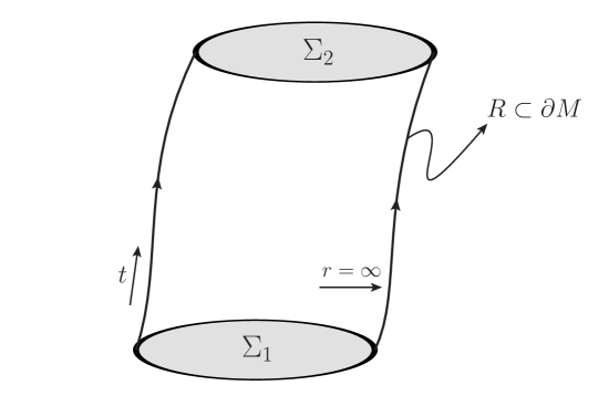
Figure 1: The symplectic structure is conserved, i.e. $\Omega(\Sigma_{1})=\Omega(\Sigma_{2})$, when the symplectic flux through the region $R\subset\partial M$ vanishes.

$$\Phi=\int_{R}d^{2}x\sqrt{|\gamma|}\,\rho_{\mu}\omega^{\mu}=0\,,$$ (3.8)

where, as before, $\rho^{\mu}$ and $\gamma$ are the unit normal and the determinant of the induced metric on $R$, respectively. We suppose that this is attained locally, so that the flux through the boundary vanishes through any open subset $R$. We mention that, from the point of view of the dual theory, these local boundary conditions correspond to the insertion of local operators. In the presence of additional boundaries, e.g. the Poincaré horizon, one must also require the flux to vanish there. Given our assumption of locality, the boundary conditions at the extra boundaries are of course independent of the ones at the conformal boundary. It is worth noting that, for black hole spacetimes, the phase space is typically defined including the interior of the black hole, so a non-vanishing flux through the horizon is not in conflict with conservation of $\Omega$.

In the coordinates introduced in (2.11) the only non-vanishing component of $\rho$ is $\rho_{r}=\sqrt{g_{rr}}=N_{r}$, where $N_{r}$ is the lapse in a radial foliation. Since $\sqrt{|g|}=N_{r}\sqrt{|\gamma|}$, we have

$$\Phi=\int_{R}d^{2}x\sqrt{|g|}\,\bar{\rho}_{\mu}\omega^{\mu}\,,$$ (3.9)

where $\bar{\rho}_{\mu}\,dx^{\mu}=dr$ and $g$ is the determinant of the full $(2+1)$ metric, as before. If we now split the connection as in (2.6), so that in an obvious notation the gauge field fluctuation is $\delta A=\delta B+\delta A^{(0)}$, we find

$$\omega^{\mu}=\omega^{\mu}_{B}+\omega^{\mu}_{0}+\omega^{\mu}_{mix}\,,$$ (3.10)

where we have defined

$$\omega^{\mu}_{B}\equiv{} -\frac{1}{q^{2}}\Bigl{(}f_{1}^{\mu\nu}\delta_{2}B_{\nu}-f_{2}^{\mu\nu}\delta_{1}B_{\nu}\Bigr{)}-\hat{\alpha}\,\epsilon^{\mu\rho\nu}\delta_{1}B_{\rho}\delta_{2}B_{\nu}$$ (3.11)

$$\omega^{\mu}_{0}\equiv{} -\hat{\alpha}\,\epsilon^{\mu\rho\nu}\delta_{1}A^{(0)}_{\rho}\delta_{2}A^{(0)}_{\nu}$$ (3.12)

$$\omega^{\mu}_{mix}\equiv{} -\frac{1}{q^{2}}\Bigl{(}f_{1}^{\mu\nu}\delta_{2}A^{(0)}_{\nu}-f_{2}^{\mu\nu}\delta_{1}A^{(0)}_{\nu}\Bigr{)}-\hat{\alpha}\,\epsilon^{\mu\rho\nu}\bigl{(}\delta_{1}A^{(0)}_{\rho}\delta_{2}B_{\nu}+\delta_{1}B_{\rho}\delta_{2}A^{(0)}_{\nu}\bigr{)}$$ (3.13)

with $f$ the field strength of $\delta B$. We now notice that contracting equation (2.8) with the Levi-Civita tensor results in $0=F_{\mu\nu}-q^{2}\hat{\alpha}\,\epsilon_{\mu\nu\rho}B^{\rho}$. Consequently, the fluctuations of the gauge-invariant mode satisfy

$$f^{\mu\nu}=q^{2}\hat{\alpha}\,\epsilon^{\mu\nu\rho}\delta B_{\rho}\,.$$ (3.14)

Using this on-shell condition in the above expression for $\omega^{\mu}$ we find

$$\omega^{\mu}_{B}=\hat{\alpha}\,\epsilon^{\mu\nu\rho}\delta_{1}B_{\nu}\delta_{2}B_{\rho}\,,\qquad\omega^{\mu}_{0}=-\hat{\alpha}\,\epsilon^{\mu\nu\rho}\delta_{1}A^{(0)}_{\nu}\delta_{2}A^{(0)}_{\rho}\,,\qquad\omega^{\mu}_{mix}=0\,.$$ (3.15)

As a result of the splitting (3.15), the symplectic structure can be written as

$$\Omega=\int_{\Sigma}d^{2}x\sqrt{h}\,n_{\mu}\omega^{\mu}_{B}+\int_{\Sigma}d^{2}x\sqrt{h}\,n_{\mu}\omega^{\mu}_{0}\,.$$ (3.16)

This suggests that the space of solutions is a direct product of the flat and non-flat sectors. However, a more detailed analysis reveals that this is only true if the boundary conditions do not mix modes in the various sectors, see section 3.2.

Let us now find an expression for the symplectic flux that will allow us to determine the allowed boundary conditions. In order to do so, it is important to keep in mind that the modes $\delta B^{(\pm)}$ are constrained by the asymptotic equations of motion, and therefore obey (2.13). For example, in light-cone coordinates $(u,v)$ in which the boundary metric takes the form

$$g^{(0)}_{ij}=\left(\begin{array}[]{cc}0&2\\ 2&0\\ \end{array}\right)$$ (3.17)

these lead to

$$\delta B_{v}^{(+)}=\delta B_{u}^{(-)}=0\,.$$ (3.18)

Taking the asymptotic constraints (2.13) into account then, we find that the symplectic flux through $R$ is given by

$$\Phi={} \hat{\alpha}\int_{R}d^{2}x\,\varepsilon^{r\nu\lambda}\left(\delta_{1}A^{(0)}_{\nu}\delta_{2}A^{(0)}_{\lambda}-\delta_{1}B_{\nu}^{(+)}\delta_{2}B_{\lambda}^{(-)}+\delta_{2}B_{\nu}^{(+)}\delta_{1}B_{\lambda}^{(-)}\right)$$

$$={} \hat{\alpha}\int_{R}d^{2}x\,\varepsilon^{ij}\left(\delta_{1}A^{(0)}_{i}\delta_{2}A^{(0)}_{j}-\delta_{1}B_{i}^{(+)}\delta_{2}B_{j}^{(-)}+\delta_{2}B_{i}^{(+)}\delta_{1}B_{j}^{(-)}\right).$$ (3.19)

3.2 Boundary conditions

As discussed above, demanding the vanishing of the symplectic flux gives us a useful way of classifying the boundary conditions. Momentarily giving up covariance in the boundary directions, in light-cone coordinates (3.17) we find that possible local boundary conditions include

$$A^{(0)}_{u}=W\bigl{[}A^{(0)}_{v}\bigr{]},\qquad B_{u}^{(+)}=V\bigl{[}B_{v}^{(-)}\bigr{]}.$$ (3.20)

For general “potentials” $W$ and $V$, such boundary conditions would correspond to multi-trace deformations in the dual CFT. For simplicity, let us focus on the linear case

$$\delta A^{(0)}_{u}=\bar{\beta}\,\delta A^{(0)}_{v},\qquad\delta B_{u}^{(+)}=\beta\,\delta B_{v}^{(-)},$$ (3.21)

for any constants $\beta,\bar{\beta}$. Note that $\beta=0,\infty$ correspond to chiral boundary conditions, while other values mix the modes and break covariance. We will refer to $\delta B_{u}^{(+)}=0$ as Dirichlet and to $\delta B_{v}^{(-)}=0$ as Neumann boundary conditions, in close analogy to the terminology commonly used for scalar fields in AdS. We will term the boundary condition $\delta B_{u}^{(+)}=\beta\,\delta B_{v}^{(-)}$ as “mixed” when $\beta$ is finite. As usual, the boundary conditions with finite $\beta$ and $\bar{\beta}$ are related to double-trace deformations of the boundary theory [25, 44], as we will review later on. Furthermore, we notice that, because $B_{u}^{(+)}$ and $B_{v}^{(-)}$ have scaling dimensions $\Delta_{-}=1-\alpha$ and $\Delta_{+}=1+\alpha$, respectively, the constant $\beta$ has dimension $\Delta_{\beta}=-2\alpha$. The RG flow interpretation of double-trace deformations has been discussed in, for example, [25, 45, 46, 47, 48]. On the other hand, since $A^{(0)}_{u}$ and $A^{(0)}_{v}$ both have dimension one, the constant $\bar{\beta}$ is dimensionless. Interestingly, we also note the possibility of a “hybrid” boundary condition

$$\delta A^{(0)}_{u}=\kappa\,\delta B_{u}^{(+)}\qquad\mbox{{and}}\qquad\delta A^{(0)}_{v}=\frac{1}{\kappa}\delta B_{v}^{(-)}\,,$$ (3.22)

that mixes the flat connections with the massive sector. Here, $\kappa$ is a constant of scaling dimension $\Delta_{\kappa}=\alpha$. Notice that, in view of the flatness condition on $\delta A^{(0)}$, (3.22) implies

$$\kappa^{2}\,\partial_{v}\delta B_{u}^{(+)}=\partial_{u}\delta B_{v}^{(-)}\,.$$ (3.23)

In analogy with the linear boundary conditions discussed above, this hybrid boundary condition has the interpretation of a double-trace deformation. To our knowledge, the possibility of such boundary conditions has not been explicitly discussed in the literature.

It is now clear from the decomposition (3.16) and the analysis of the boundary conditions above that, as anticipated in [18], the flat and massive sectors do not always decouple. In fact, for our hybrid boundary conditions (3.22) both sectors indeed interact with one another. The decoupling only occurs if one imposes boundary conditions which do not mix both sectors, i.e. if we impose boundary conditions like those in (3.21). This is because it is only in this case that the symplectic structure effectively splits as a direct sum of two independent pieces.

3.3 One-point functions

As usual in the context of holography, the Maxwell-Chern Simons action (2.1) must be supplemented by a series of boundary terms that serve two purposes: achieving a well-defined variational principle for a chosen set of boundary conditions, and removing divergences. We will refer to the latter as counterterms. We recall now that the first variation of the bulk action is given by (3.3). Evaluating this expression on-shell we find

$$\left.\delta I\right|_{os}=\frac{\hat{\alpha}}{2}\int_{\partial M}d^{2}x\,\sqrt{|\gamma|}\,\rho_{\mu}\epsilon^{\mu\rho\nu}\left(B_{\rho}-A^{(0)}_{\rho}\right)\delta A_{\nu}\,,$$ (3.24)

where the gauge field fluctuations are understood to be evaluated on the solution of the linearized equations of motion. Employing the notation established above, we find

$$\left.\delta I\right|_{os}={} -\frac{\hat{\alpha}}{2}\int_{\partial M}d^{2}x\,\varepsilon^{ij}\left(B_{i}-A^{(0)}_{i}\right)\left(\delta A^{(0)}_{j}+\delta B_{j}\right)$$

$$={} -\frac{\hat{\alpha}}{2}\int_{\partial M}d^{2}x\,\varepsilon^{ij}\left(B^{(+)}_{i}\delta B_{j}^{(-)}+B_{i}^{(-)}\delta B_{j}^{(+)}-A^{(0)}_{i}\delta A^{(0)}_{j}\right)$$

$$-\frac{\hat{\alpha}}{2}\lim_{r\to\infty}\int_{\partial M}d^{2}x\,\varepsilon^{ij}r^{\alpha}\left(B_{i}^{(+)}\delta A^{(0)}_{j}+A_{j}^{(0)}\delta B_{i}^{(+)}\right)\,,$$ (3.25)

where in the last equality we used the restrictions placed by the asymptotic equations of motion on the $B^{(\pm)},\delta B^{(\pm)}$ modes (c.f. section 2.1). We note the presence (for any finite Maxwell coupling $q^{2}$) of the divergent term, which we cancel by the addition of a counterterm. Noticing that $\varepsilon^{ij}r^{\alpha}\left(B_{i}^{(+)}\delta A^{(0)}_{j}+A_{j}^{(0)}\delta B_{i}^{(+)}\right)=\delta\left(r^{\alpha}\varepsilon^{ij}A_{j}^{(0)}B_{i}^{(+)}\right)$ it is easy to check that the desired counterterm is given by the covariant expression

$$I_{ct}=\frac{1}{2q^{2}}\int_{\partial M}d^{2}x\sqrt{|\gamma|}F^{i}A_{i}\,,$$ (3.26)

where, as before, $\gamma$ is the determinant of the induced metric on the $r={\rm constant}$ surface, and we have defined

$$F^{i}\equiv\rho_{\mu}F^{\mu i}\,,$$ (3.27)

with $\rho_{\mu}$ the unit normal 1-form on the radial slices. Therefore, we have that

$$\left.\delta\left(I+I_{ct}\right)\right|_{os}={} -\frac{\hat{\alpha}}{2}\int_{\partial M}d^{2}x\,\varepsilon^{ij}\left(B^{(+)}_{i}\delta B_{j}^{(-)}+B_{i}^{(-)}\delta B_{j}^{(+)}-A^{(0)}_{i}\delta A^{(0)}_{j}\right)$$ (3.28)

is finite as $r\to\infty$.

3.3.1 Covariant boundary conditions

In order to proceed further we need to discuss the additional finite boundary terms needed in order to enforce different boundary conditions of interest. Confining ourselves to covariant terms for the moment, we consider the following quantities:

$$B_{\pm}={} \mp\frac{1}{4q^{4}\hat{\alpha}}\int_{\partial M}d^{2}x\sqrt{|\gamma|}F^{i}\gamma_{ij}F^{j}\,,$$ (3.29)

$$B_{(0)}={} \frac{1}{2q^{2}}\int_{\partial M}d^{2}x\,\varepsilon^{ij}F_{i}A_{j}+\frac{1}{4}\int_{\partial M}d^{2}x\sqrt{|\gamma|}\gamma^{ij}\left(\frac{1}{q^{4}\hat{\alpha}}F_{i}F_{j}-\hat{\alpha}A_{i}A_{j}\right)\,.$$ (3.30)

Evaluating on-shell we find

$$\left.B_{\pm}\right|_{os}={} \pm\frac{\hat{\alpha}}{2}\int_{\partial M}d^{2}x\sqrt{|g^{(0)}|}g^{(0)ij}B_{i}^{(-)}B_{j}^{(+)}$$

$$={} \pm\frac{\hat{\alpha}}{2}\int_{\partial M}d^{2}x\,\varepsilon^{ij}B_{i}^{(+)}B_{j}^{(-)}$$ (3.31)

$$\left.B_{(0)}\right|_{os}={} -\frac{\hat{\alpha}}{4}\int_{\partial M}d^{2}x\sqrt{|g^{(0)}|}g^{(0)ij}A_{i}^{(0)}A_{j}^{(0)}\,.$$ (3.32)

By taking linear combinations of these finite boundary terms we can achieve a variational principle well-suited for the various boundary conditions (3.21) of interest in the flat and gauge-invariant (massive) sectors. For example, we find

$$\delta\left.\left(I+I_{ct}\pm B_{(0)}+B_{+}\right)\right|_{os}={} \hat{\alpha}\int_{\partial M}d^{2}x\sqrt{|g^{(0)}|}\left[\epsilon^{ij}B_{i}^{(-)}\delta B_{j}^{(+)}\mp A_{i}^{(0)}P_{\pm}^{ij}\delta A^{(0)}_{j}\right]\,,$$ (3.33)

and

$$\delta\left.\left(I+I_{ct}\pm B_{(0)}+B_{-}\right)\right|_{os}={} \hat{\alpha}\int_{\partial M}d^{2}x\sqrt{|g^{(0)}|}\left[\epsilon^{ij}B^{(+)}_{i}\delta B_{j}^{(-)}\mp A_{i}^{(0)}P_{\pm}^{ij}\delta A^{(0)}_{j}\right].$$ (3.34)

Now that we have identified the sources for the covariant boundary conditions, i.e. $\delta B^{(\pm)}_{i}$ and $\left(P_{\pm}\delta A^{(0)}\right)_{i}=g^{(0)}_{ij}P_{\pm}^{jk}\delta A^{(0)}_{k}$, we write the variation of the renormalized action $I_{ren}$ generically as

$$\left.\delta I_{ren}\right|_{os}=\int_{\partial M}d^{2}x\sqrt{|g^{(0)}|}\biggl{[}\langle\mathcal{O}^{(\pm)i}\rangle\delta B^{(\pm)}_{i}+\langle\mathcal{O}_{\pm}^{(0)\,i}\rangle\left(P_{\pm}\delta A^{(0)}\right)_{i}\biggr{]}.$$ (3.35)

Comparing with (3.33) and (3.34) and using the properties of $P_{\pm}$ we can read-off the one-point functions of the dual operators, and we obtain

$$\langle\mathcal{O}^{(\pm)i}\rangle={} \pm\hat{\alpha}\,g^{(0)ij}B_{j}^{(\mp)}\,,$$ (3.36)

$$\langle\mathcal{O}_{\pm}^{(0)\,i}\rangle={} \mp\hat{\alpha}P_{\mp}^{ij}A_{j}^{(0)}\,.$$ (3.37)

Since $A_{i}^{(0)}$ is constrained by the flatness condition, the variational derivatives with respect to its components are ill-defined, and, as a consequence, the one-point functions (3.37) suffer from an ambiguity. However, this ambiguity is nothing but the one associated to the $U(1)$ gauge transformations. In other words, (3.37) are only defined up to the transformations $\delta A_{i}=\partial_{i}\lambda$ that preserve the boundary conditions in the variational principle. See [19] for a related discussion in the context of (pure) Maxwell fields.

3.3.2 Symmetry-breaking boundary conditions

Let us now turn to the less symmetric scenarios. First, we consider the case of “mixed” boundary conditions, i.e. $B^{(+)}_{u}-\beta B^{(-)}_{v}=0$, where $\beta$ is a finite dimensionful constant. It is clear that this requirement breaks both conformal and Poincaré symmetry, so we are allowed to write down the appropriate boundary terms simply in terms of the coefficients of the asymptotic expansion. As we shall see shortly, it is useful to generalize the above boundary condition and consider instead

$$B^{(+)}_{u}-\beta B^{(-)}_{v}=J_{\beta}\,,$$ (3.38)

where $J_{\beta}$ is an arbitrary fixed function of the boundary coordinates. We ignore the contribution from the flat sector momentarily. Starting from the Neumann theory, i.e. the theory in which $B^{(-)}_{i}$ is fixed and whose action we denote by $I_{N}$, the boundary term we need to add in order to attain the mixed boundary condition is

$$I_{def,\beta}=-\frac{\hat{\alpha}}{4\beta}\int_{\partial M}d^{2}x\sqrt{|g^{(0)}|}\left(B^{(+)}_{u}\right)^{2}\,.$$ (3.39)

In fact, using the variation of the Neumann action (3.34) and the explicit boundary term (3.39), we obtain

$$\delta\left(I_{N}+I_{def,\beta}\right)=\frac{\hat{\alpha}}{2\beta}\int_{\partial M}d^{2}x\sqrt{|g^{(0)}|}B^{(+)}_{u}\left(\beta\,\delta B^{(-)}_{v}-\delta B^{(+)}_{u}\right),$$ (3.40)

which is finite and stationary when the boundary condition (3.38) holds. Comparing (3.40) with (3.38), we note that the quantity that is being held fixed in the variational principle is in fact $J_{\beta}$. This means that $J_{\beta}$ is to be interpreted as the source for the dual operator in the boundary theory. Given this, it follows from (3.40) that the one-point function in the presence of sources for the dual operator in the deformed theory is given by

$$\langle{\cal O}^{(-)}_{u}\rangle_{\beta}=-\frac{\hat{\alpha}}{2\beta}B^{(+)}_{u},$$ (3.41)

where, as usual, $B^{(+)}_{u}$ must be thought of as a function of the source $J_{\beta}$ defined in (3.38). Before constructing variational principles suitable for the remaining boundary conditions, we comment that the computation above provides a simple illustration of the well-known fact that linear boundary conditions of the form (3.38) correspond to double-trace deformations in the dual theory. The argument is as follows. First, we recall that in AdS/CFT the Neumann action $I_{N}$ is interpreted as the generating function for the operator associated to $B^{(+)}_{u}$ in the dual CFT. Then, the boundary term (3.39) is transparently identified with a double-trace deformation for this operator. Moreover, the inclusion of (3.39) implies that the original Neumann boundary condition needs to be shifted in such a way that the the modified action has an extremum. As noted above, the new boundary condition is nothing but the linear relation (3.38), which completes the argument. It is worth commenting on the possibility of thinking of the (3.38) as a deformation of the Dirichlet theory. In such case, the boundary term that implements the shift in the boundary condition is quadratic in $B^{(-)}_{v}$, so it has dimension $2(1+\alpha)$. We see that the deformation is then irrelevant.

We now construct an appropriate action for the boundary condition

$$A^{(0)}_{u}-\bar{\beta}A^{(0)}_{v}=J_{\bar{\beta}}$$ (3.42)

where $\bar{\beta}$ is a non-zero dimensionless constant and $J_{\bar{\beta}}$ is a fixed arbitrary function of the boundary coordinates. In analogy with the previous case, $J_{\bar{\beta}}$ corresponds to the source of the dual operator. Note that since $\bar{\beta}$ is dimensionless the boundary condition (3.42) for $J_{\bar{\beta}}=0$ preserves scale invariance, yet it breaks Lorentz invariance. Once again, as a consequence of this, it is licit to write extra boundary terms which are not Lorentz densities. Moreover, because this boundary condition does not mix the flat and massive sectors, we concentrate on the flat connections and temporarily drop the contribution from the massive modes. Now, assuming that we start with an action $I^{(1)}_{ren}$ which attains an extremum when $P_{-}A^{(0)}$ is fixed, we find

$$\delta I^{(1)}_{ren}=\hat{\alpha}\int_{\partial M}d^{2}x\sqrt{|g^{(0)}|}\langle\mathcal{O}_{-}^{(0)\,i}\rangle(P_{-}\delta A^{(0)})_{i}=\frac{\hat{\alpha}}{2}\int_{\partial M}d^{2}x\sqrt{|g^{(0)}|}A^{(0)}_{u}\delta A^{(0)}_{v}$$ (3.43)

as follows from (3.35) and (3.37). In this case, the boundary term that we need to add to $I^{(1)}_{ren}$ in order for (3.42) to hold can be written as

$$I_{def,\bar{\beta}}=-\frac{\hat{\alpha}}{4\bar{\beta}}\int_{\partial M}d^{2}x\sqrt{|g^{(0)}|}\left(A^{(0)}_{u}\right)^{2}\,.$$ (3.44)

In fact, with this choice the on-shell variation of the action reads

$$\delta\left(I^{(1)}_{ren}+I_{def,\bar{\beta}}\right)=\frac{\hat{\alpha}}{2\bar{\beta}}\int_{\partial M}d^{2}x\sqrt{|g^{(0)}|}A^{(0)}_{u}\left(\bar{\beta}\delta A^{(0)}_{v}-\delta A^{(0)}_{u}\right),$$ (3.45)

as desired. As discussed above, the boundary condition (3.42) is in one-to-one correspondence with the inclusion of the double-trace deformation (3.44) in the dual theory. The relevant one-point function is given by

$$\langle{\cal O}^{(0)}_{+u}\rangle_{\bar{\beta}}=-\frac{\hat{\alpha}}{2\bar{\beta}}A^{(0)}_{u}\,.$$ (3.46)

Once again, we mention that the one-point function (3.46) is only defined up to the appropriate $U(1)$ transformation.

Finally, we consider the “hybrid” boundary conditions defined in (3.22), which admit the obvious generalization

$$A^{(0)}_{u}-\kappa B^{(+)}_{u}=J_{\kappa}\,,\qquad A^{(0)}_{v}-\kappa^{-1}B^{(-)}_{v}=\tilde{J}_{\kappa}\,,$$ (3.47)

where we take $J_{\kappa}$, $\tilde{J}_{\kappa}$ to be the sources of the dual operators. It is convenient to start with a renormalized action $I^{(2)}_{ren}$ such that

$$\delta I^{(2)}_{ren}=\frac{\hat{\alpha}}{2}\int_{\partial M}d^{2}x\sqrt{|g^{(0)}|}\left(A^{(0)}_{u}\delta A^{(0)}_{v}+B^{(-)}_{v}\delta B^{(+)}_{u}\right).$$ (3.48)

With $I^{(2)}_{ren}$ as a starting point, the boundary term that implements hybrid boundary conditions is given by

$$I_{def,\kappa}=-\frac{\hat{\alpha}}{2\kappa}\int_{\partial M}d^{2}x\sqrt{|g^{(0)}|}B^{(-)}_{v}A^{(0)}_{u},$$ (3.49)

as it follows from

$$\delta\left(I^{(2)}_{ren}+I_{def,\kappa}\right)={} \frac{\hat{\alpha}}{2}\int_{\partial M}d^{2}x\sqrt{|g^{(0)}|}A^{(0)}_{u}\left(\delta A^{(0)}_{v}-\kappa^{-1}\delta B^{(-)}_{v}\right)$$

$$-\frac{\hat{\alpha}}{2}\int_{\partial M}d^{2}x\sqrt{|g^{(0)}|}\kappa^{-1}B^{(-)}_{v}\left(\delta A^{(0)}_{u}-\kappa\,\delta B^{(+)}_{u}\right).$$ (3.50)

As pointed out before, the hybrid boundary conditions correspond to a double-trace deformation in the dual theory. Note that, in this case, the deformation (3.49) explicitly mixes the flat and massive sectors, so indeed these do not decouple in the theory defined by the hybrid boundary conditions. It follows from (3.3.2) that the one-point functions in the dual theory are given by

$$\langle{\cal O}^{(0)}_{+u}\rangle_{\kappa}=\frac{\hat{\alpha}}{2}A^{(0)}_{u}\qquad\mbox{and}\qquad\langle{\cal O}^{(0)}_{-v}\rangle_{\kappa}=-\frac{\hat{\alpha}}{2\kappa}B^{(-)}_{v}\,.$$ (3.51)

It is worthwhile noting that, since the $U(1)$ transformations do not preserve the boundary conditions (3.22), the one-point functions (3.51) are unambiguously defined.

Before closing this section, we emphasize that, provided $0<\alpha<1$, the boundary terms involved do not contain derivatives along the timelike direction. Given the results of [43], this strongly suggests that the bulk symplectic structure does not need to be supplemented by additional boundary contributions. This is indeed the case, as we will explicitly verify below. Specifically, we will check that, for $0<\alpha<1$, the bulk symplectic structure is finite and conserved for all the boundary conditions under scrutiny.

3.4 The symplectic product

Recall that the symplectic structure is given by (3.16) with (3.15), i.e.

$$\Omega=\hat{\alpha}\int_{\Sigma}d^{2}x\sqrt{h}n_{\mu}\epsilon^{\mu\nu\rho}\delta_{1}B_{\nu}\delta_{2}B_{\rho}-\hat{\alpha}\int_{\Sigma}d^{2}x\sqrt{h}n_{\mu}\epsilon^{\mu\nu\rho}\delta_{1}A^{(0)}_{\nu}\delta_{2}A^{(0)}_{\rho}\,.$$ (3.52)

As mentioned above, it turns out that the restriction $0<\alpha<1$ ensures that (3.52) is finite for all the boundary conditions of interest, provided one imposes additional requirements on the solutions in the deep interior.

Quite generally, given a symplectic structure it is possible to endow the space of solutions with an inner product defined in terms of $\Omega$, as we now review briefly. A more detailed discussion can be found in [38], for example. We start by complexifying the space of solutions and consider

$$(A_{1},A_{2})=-i\Omega(A_{1}^{*},A_{2})\,.$$ (3.53)

We will refer to (3.53) as the symplectic product of the theory. One can verify that (3.53) satisfies the expected properties of bi-linearity and Hermiticity, although in general it fails to be positive definite.

The inner product (3.53) allows us to introduce some useful terminology. First, we shall term a given solution $A_{0}$ as normalizable if $(A_{0},A)$ is finite for all $A$. As stated above, in our particular setup this translates into a requirement on the fields in the deep interior. Second, we define a ghost to be an excitation of definite positive(negative) frequency with negative(positive) norm. Here, we will use the definition of positive frequency associated to the timelike Killing vector of the relevant background geometry under consideration. For example, if $\partial_{t}$ is a vector field which is timelike everywhere, the solution $A$ is said to be a positive frequency solution if $\partial_{t}A=-i\omega A$ with $\omega>0$. Third, we will refer to a solution $A_{gauge}$ as pure gauge if $(A_{gauge},A)=0$ for all $A$.

It should be noted that the presence of ghosts in a given system is correlated with the lack of unitarity in the associated quantum theory. At the classical level, the presence of ghosts also signals pathologies since these give negative contributions to the energy.

4 The dual field theory spectrum

In this section we determine the spectrum of normalizable solutions of the MCS system in $AdS_{3}$, in both global and Poincaré coordinates, for the various boundary conditions of interest. As explained in section 3.4, by “normalizable” we mean excitations that have finite symplectic product with all the modes. We mention that, while normalizability at the conformal boundary is guaranteed by restricting the coupling $\alpha$ defined in (2.3) to satisfy $0<\alpha<1$, normalizability at the interior is achieved by restricting the wave functions appropriately. More precisely, when the geometry is global AdS we shall require the wave functions to be smooth at the origin, as is customary. In the Poincaré AdS case, in addition to smoothness in the interior, we restrict the wave functions in such a way that no symplectic flux can leak through the Poincaré horizon.

As explained in section 2, the connection splits into flat and “massive” pieces, and we can solve the bulk equations of motion separately for each sector. Moreover, as discussed in section 3.2, these sectors decouple unless we impose the “hybrid” boundary condition (3.22). Our strategy to find the spectrum will be to focus on the massive and flat sectors separately, and incorporate the effects of the mixing only when we discuss the hybrid boundary conditions. For the sake of simplifying the exposition, we display the general solution to the equations of motion of the massive mode in appendix A, while here we focus exclusively on imposing the appropriate boundary conditions.

4.1 Global $AdS_{3}$

We first consider the MCS theory in global $AdS_{3}$, whose line element is given by (A.17). Since the spacetime is topologically trivial, there is no room for holonomies and the connection must be smooth at the origin, where the vector field $\partial_{x}=(1/L)\partial\varphi$ becomes singular. As a result, in addition to normalizability we must impose $A[\partial_{x}]=A_{x}=0$ at $\rho=0$. It should be stressed that setting $A^{(0)}_{\rho}=0$ everywhere in the bulk is generically in conflict with smoothness. To see why, we note that this implies that the components of $A^{(0)}$ along the boundary directions are independent of $\rho$ everywhere, so any boundary condition other than $A^{(0)}_{x}|_{\partial M}=0$ would yield singular configurations. Having said this, we initiate the study of the spectrum for all the boundary conditions of interest.

4.1.1 Flat sector

We first consider the flat sector. Since there are no holonomies, the flat connections can be written as

$$\delta A^{(0)}_{\mu}=\partial_{\mu}\lambda\,,$$ (4.1)

where $\lambda$ is smooth everywhere, with $\partial_{x}\lambda=0$ at $\rho=0$. Recall that in our analysis of the symplectic flux, we encountered the allowed boundary condition (3.21), which in terms of the $(t,x)$ coordinates defined in appendix A takes the form

$$\left.\left(\delta A^{(0)}_{t}-\hat{\beta}\,\delta A^{(0)}_{x}\right)\right|_{\partial M}=0\,,$$ (4.2)

where $\hat{\beta}=(\bar{\beta}-1)/(\bar{\beta}+1)$ is a (possibly vanishing or infinite) constant. Fourier-decomposing $\lambda$ as $\lambda=e^{-i\omega t+ikx}\hat{\lambda}(k,\omega)$ with $k\in\mathds{Z}$, and using (4.1) in (4.2), we learn that the frequencies must satisfy

$$\omega=-\hat{\beta}k\,,$$ (4.3)

which determines the spectrum of the flat sector. As is well-known [11, 12, 13, 10, 14, 15, 16, 17], the degrees of freedom of the flat sector reside exclusively on the spacetime boundary, a fact that we will briefly review in appendix C. We will consider the flat solutions for hybrid boundary conditions in the next subsection.

4.1.2 Massive sector

Focusing now on the massive sector we use the ansatz (A.18), in which case the solution is given by (A.21)-(A.26) in terms of functions $F(\omega,\pm k,\pm\alpha;\rho)$. We observe that only the $F(\omega,|k|,\alpha;\rho)$ profiles are regular in the interior ($\rho\to 0$). Hence, for $k<0$, we take the $F(\omega,-k,\alpha;\rho)$ solution. Consequently, we will write the general solution which is smooth in the interior of $AdS_{3}$ as

$$b_{u}={} C_{u}F(\omega,|k|,\alpha;\rho)$$ (4.4)

$$b_{v}={} C_{v}F(\omega,|k|,-\alpha;\rho)\,,$$ (4.5)

where $(u,v)$ are the light-cone coordinates defined in (A.4), $F(\omega,k,\alpha;\rho)$ is defined as in (A.23), and

$$\frac{C_{v}}{C_{u}}=\frac{k+\omega-s(k)\alpha}{k-\omega+s(k)\alpha}\,.$$ (4.6)

Here, $s$ denotes the sign function, i.e. $s(k)=1$ for $k\geq 0$ and $s(k)=-1$ for $k<0$. The $b_{\rho}$ component is obtained from $b_{u}$ and $b_{v}$ via (A.24) and it is subleading with respect to them near the conformal boundary of $AdS_{3}$. Expanding $F(\omega,k,\alpha;\rho)$ near $\rho=\infty$ and using (4.4)-(4.6), we learn that the relevant coefficients in the asymptotic expansion are

$$b^{(+)}_{u}={} C_{u}C(\alpha,|k|,\omega)\,, b^{(+)}_{v}={} 0\,,$$ (4.7)

$$b^{(-)}_{v}={} C_{u}\frac{k+\omega-s(k)\alpha}{k-\omega+s(k)\alpha}C(-\alpha,|k|,\omega)\,, b^{(-)}_{u}={} 0\,,$$ (4.8)

where

$$C(\alpha,k,\omega)=\frac{\Gamma(k+1)\Gamma(1+\alpha)}{\Gamma\left(\displaystyle{1+\frac{k+\alpha-\omega}{2}}\right)\Gamma\left(\displaystyle{1+\frac{k+\alpha+\omega}{2}}\right)}\,.$$ (4.9)

A choice of asymptotic boundary conditions will constrain the allowed values of $(\omega,k)$, corresponding to the normal modes of the system. In the Dirichlet case $(\beta=0)$ the source is identified with $b^{(+)}_{u}$ and the normal modes are given by the zeros of $C(\alpha,|k|,\omega)$, located at

$$\omega^{\pm}_{nk}=\pm\left(2n+|k|+\alpha\right)\,,\qquad n=1,2,\ldots$$ (4.10)

and the zeros of the denominator in (4.6), located at

$$\omega^{+}_{0k}={} +(|k|+\alpha) {\rm for}\ k>0$$ (4.11)

$$\omega^{-}_{0k}={} -(|k|+\alpha) {\rm for}\ k<0\,.$$ (4.12)

We notice that the normal modes with $n\geq 1$ are doubly degenerate, with each frequency attained for both $k$ and $-k$, while $\omega^{\pm}_{0k}$ occur only once.

Similarly, for Neumann boundary condition $(b^{(-)}_{v}=0)$ we find the eigenfrequencies

$$\omega^{\pm}_{nk}=\pm\left(2n+|k|-\alpha\right)\,,\qquad n=1,2,\ldots$$ (4.13)

in addition to

$$\omega^{-}_{0k}={} \alpha-|k| {\rm for}\ k>0$$ (4.14)

$$\omega^{+}_{0k}={} |k|-\alpha {\rm for}\ k<0\,.$$ (4.15)

More generally, the boundary condition $b^{(+)}_{u}=\beta\,b^{(-)}_{v}$ for finite $\beta$ gives

$$C(\alpha,|k|,\omega)-\beta\frac{k+\omega-s(k)\alpha}{k-\omega+s(k)\alpha}C(-\alpha,|k|,\omega)=0\,.$$ (4.16)

For generic $\beta$, we will proceed numerically, examining the structure of the solutions of (4.16) in the complex-$\omega$ plane as a function of $k$, $\beta$ and $\alpha$. For $\beta>0$ and all values of $k$, we find an infinite discrete set of real frequency solutions, in analogy to the Dirichlet and Neumann cases. Now, while for $\beta<0$ and $k>0$ all frequencies are real, for $\beta<0$ and $k<0$ a pair of complex solutions occurs in addition to the series of real solutions. Notice that, with the exception of $\omega$, all the parameters in (4.16) are real, which implies that complex solutions must appear in complex conjugate pairs. These complex solutions go off to $\pm i\infty$ as $\beta\rightarrow 0$, in agreement with our analysis for Dirichlet boundary conditions. See figures 2 and 2. The complex frequency solutions signal an instability of the system, since some perturbations can grow exponentially with time. This instability is associated with ghosts, as we will see in section 5.2. We stress that, aside from the existence of complex frequencies, there is nothing particularly special about $\beta<0$. In fact, we will see below that all values of $\beta\neq 0$ are qualitatively equivalent, since they all yield ghosts.

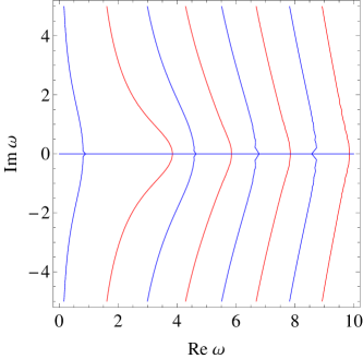
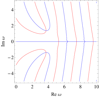
Figure 2: 2: We plot in red/blue the solution of the real/imaginary part of equation (4.16) in the complex-$\omega$ plane for $\{k=2,\,\alpha=0.2,\,\beta=1.7\}$. We observe that these solutions only intersect for $\mbox{Im}(\omega)=0$, which illustrates the fact that (4.16) has only real solutions for $\beta>0$. 2: For $\{k=-2,\,\alpha=0.2,\,\beta=-1.7\}$, we plot in red/blue the solution of the real/imaginary part of equation (4.16) in the complex-$\omega$ plane. We note that in this case there are complex frequency solutions.

Finally, we consider the hybrid boundary conditions (3.22). As noted in section 3.2, the condition (3.22) along with the flatness of $\delta A^{(0)}$ imply the extra requirement (3.23), which in view of our mode decomposition translates into

$$\kappa^{2}\frac{k+\omega}{k-\omega}C(\alpha,|k|,\omega)-\frac{k+\omega-s(k)\alpha}{k-\omega+s(k)\alpha}C(-\alpha,|k|,\omega)=0\,.$$ (4.17)

Thus, the spectrum of frequencies is given by the solutions of (4.17) provided the flat components of the connection are related to the massive ones by (3.22). Lacking an analytic solution of (4.17) for finite $\kappa$, we proceed numerically. Studying (4.17) for various values of the parameters, we find that generically there is an infinite set of real solutions. Additionally, a pair of complex solutions occurs when $k>0$ and $|\kappa|>|\kappa_{c}|$, where $\kappa_{c}$ is an increasing function of $\alpha$ and $k$. See figures 3, 3 for an illustration of this fact. We have also verified numerically that the complex solutions go off to $\pm i\infty$ as $|\kappa|$ approaches infinity, consistent with the Dirichlet result. As in the case of mixed boundary conditions, the complex frequency solutions correspond to a dynamical instability of the system that is associated to ghosts. We shall also find that the all finite values of $\kappa$ yield ghosts, in agreement with the CFT unitarity bound.

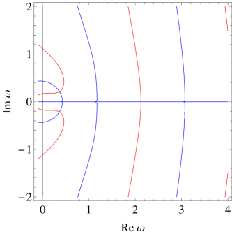
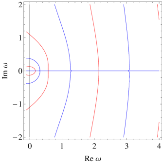
Figure 3: 3: We plot in red/blue the solution of the real/imaginary part of equation (4.17) in the complex-$\omega$ plane for $\{k=1,\,\alpha=0.8,\,\kappa=1.0\}$. We note that there are real solutions but also a pair of complex solutions near $|\omega|=0$. 3: Solutions for $\{k=1,\,\alpha=0.8,\,\kappa=0.9\}$. We observe that the complex solutions become real, which shows that for $\alpha=0.8$ the critical value of $\kappa$ is near $|\kappa_{c}|=0.95\,$.

As mentioned above, given a solution of (4.17) the components of the flat connection are uniquely determined by (3.22). It is worth mentioning that with these boundary conditions the chiral currents acquire a non-vanishing expectation value. See section 3.3.

4.2 Poincaré patch of $AdS_{3}$

We now carry out the study of the spectrum of normalizable excitations for the boundary conditions of interest in the Poincaré patch of $AdS_{3}$. As in the global AdS case, normalizability at the conformal boundary is guaranteed by the restriction $0<\alpha<1$. On the other hand, the treatment of the Poincaré horizon turns out to be more delicate as we will discuss in detail below.

4.2.1 Flat sector

Let us first consider the flat sector. As mentioned in section 3.1, when the geometry is the Poincaré patch of $AdS_{3}$, symplectic flux can generically leak through the Poincaré horizon. In the flat sector, the easiest way to see this is to note that in this sector the theory is actually topological, so there is no difference between the Poincaré horizon and the conformal boundary. From our experience with the latter, we conclude that good boundary conditions in the flat sector correspond to fixing half of the connection on the Poincaré horizon. We will impose the condition

$$\left.\delta A^{(0)}_{x}\right|_{z=\infty}=0\,.$$ (4.18)

As reviewed in appendix C, when fixing the spatial part of $A^{(0)}_{i}$, the degrees of freedom that reside at the Poincaré horizon become pure gauge, which allows us to focus on the physics at the boundary. Note however that (4.18) can be generalized in the same way as the boundary conditions discussed in section 3.2. Also, in analogy with the global case, we see that $U(1)$ transformations that set $A_{z}=0$ everywhere in the bulk generically do not preserve the boundary condition (4.18), so they are not allowed symmetries of the system.

From the above discussion, it is clear that the spectrum of the flat connections in the Poincaré case is analogous to the one in global AdS discussed in section 4.1. In particular, the frequencies are fixed as (4.3) as a consequence of the boundary conditions at the conformal boundary, which are identical to the ones we consider in the Poincaré patch. Note however that in the present case the spatial momentum $k$ is not quantized, so the spectrum of eigenfrequencies is continuous.

4.2.2 Massive sector

Let us now focus on the massive sector. In order to solve the equations of motion, we use the mode decomposition $\delta B_{\mu}=e^{i(k_{u}u+k_{v}v)}b_{\mu}\,$; see appendix A.1 for the explicit solutions. We classify the modes according to the value of $m^{2}:=-k_{u}k_{v}=\omega^{2}-k^{2}$ as: timelike ($m^{2}>0$), lightlike ($m^{2}=0$), and spacelike $(m^{2}<0)$.

From (2.12) it follows that the asymptotic expansion of the solution for the massive mode reads (after noting that near the boundary we have $r=1/z$)

$$b_{\mu}=z^{-\alpha}b^{(+)}_{\mu}+z^{\alpha}b^{(-)}_{\mu}+\mathcal{O}\left(z^{1-\alpha}\right).$$ (4.19)

Here $z$ is the radial variable defined in (A.2). Note that under the isometry (A.3), the coefficients in (4.19) scale as

$$b^{(+)}_{\mu}\rightarrow c^{\alpha-1}b^{(+)}_{\mu}~{},\qquad b^{(-)}_{\mu}\rightarrow c^{-\alpha-1}b^{(-)}_{\mu}~{},$$ (4.20)

in agreement with our discussion of section 2.2 regarding the conformal dimensions of the dual operators.

Having said this, let us consider the spectrum of timelike modes, whose radial profile is given by (A.13). Comparing (A.13) with (4.19), we read-off

$$b^{(+)}_{u}={} k_{u}C(\vec{k})\frac{2^{1+\alpha}m^{-(\alpha+1)}}{\Gamma(-\alpha)}\,, b^{(+)}_{v}={} b^{(+)}_{z}=0\,,$$ (4.21)

$$b^{(-)}_{v}={} k_{v}A(\vec{k})\frac{2^{1-\alpha}m^{\alpha-1}}{\Gamma(\alpha)}\,, b^{(-)}_{u}={} b^{(-)}_{z}=0\,.$$ (4.22)

Thus, $C(\vec{k})=0$ corresponds to Dirichlet and $A(\vec{k})=0$ to Neumann boundary conditions. We also find that mixed boundary conditions imply

$$C(\vec{k})=\beta\frac{k_{v}}{k_{u}}\frac{\Gamma(-\alpha)}{4^{\alpha}\Gamma(\alpha)}m^{2\alpha}A(\vec{k})\,,$$ (4.23)

while hybrid boundary condition translate into

$$C(\vec{k})=\kappa^{-2}\frac{\Gamma(-\alpha)}{4^{\alpha}\Gamma(\alpha)}m^{2\alpha}A(\vec{k})\,.$$ (4.24)

We stress that the timelike modes above oscillate rapidly near $z=\infty$. As a result, one can construct wave packets that behave smoothly near the Poincaré horizon. Alternatively, one can work with the modes as they stand and treat their symplectic products in the appropriate distributional sense, and this is the strategy we adopt below. More precisely, in section 5.3 we find that the timelike modes are in fact (plane wave-)normalizable for all the boundary conditions of interest.

We now study the existence of spacelike solutions, whose profiles are given by (A.14). Taking $\mbox{Re}(p)>0$ by convention, we see that unless we set $C(\vec{k})=0$ in (A.14), the solutions blow up exponentially at the horizon ($z=\infty$) and are thus non-normalizable. Therefore, we set $C(\vec{k})=0$ which implies that the coefficients of the asymptotic expansion for the spacelike solution can be written as

$$b^{(+)}_{u}={} A(\vec{k})k_{u}2^{\alpha}p^{-\alpha-1}\Gamma(1+\alpha)\,, b^{(+)}_{v}={} b^{(+)}_{z}=0\,,$$ (4.25)

$$b^{(-)}_{v}={} A(\vec{k})k_{v}2^{-\alpha}p^{\alpha-1}\Gamma(1-\alpha)\,, b^{(-)}_{u}={} b^{(-)}_{z}=0\,.$$ (4.26)

Both Dirichlet and Neumann boundary conditions require $A(\vec{k})=0$, so in these cases spacelike solutions do not exist. Mixed boundary conditions $b^{(+)}_{u}=\beta b^{(-)}_{v}$, in turn, imply the relation

$$\tilde{\beta}=\frac{(k-\omega)^{1-\alpha}}{(k+\omega)^{1+\alpha}}\,,$$ (4.27)

where we have defined $\tilde{\beta}=4^{-\alpha}\frac{\Gamma(1-\alpha)}{\Gamma(1+\alpha)}\beta$. Spacelike solutions are then in one-to-one correspondence with the solutions of (4.27), which we now study. First, we observe that regularity at transverse infinity, $|x|\rightarrow\infty$, requires $k\in\mathbb{R}$. On the other hand, recall that we derived (4.27) only under the assumption $\mbox{Re}(p)>0$, so in principle complex frequency solutions are allowed and their existence is exclusively dictated by (4.27). Examining (4.27) it is not hard to conclude that for all $\beta>0$ there are real solutions in the region $k-\omega>0$, $k+\omega>0$; see figure 4. On the other hand, if $\beta<0$ real solutions are ruled out, but we find instead a pair of complex-frequency solutions that are conjugate to each other, see figure 4. The fact that our results depend on the sign of $\beta$ only can be easily understood in terms of the scaling symmetry (A.3), which acts non-trivially on $\beta$.

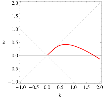
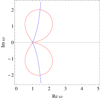
Figure 4: 4: We plot in red the real solutions of (4.27) in the $(k,\omega)$ plane for $\{\tilde{\beta}=0.5\,,\alpha=0.6\}$. The dashed line corresponds to the light-cone in momentum space. 4: For $\{\tilde{\beta}=-0.5,\,\alpha=0.6,\,k=-1\}$, we plot in red/blue the solutions to the real/imaginary part of (4.27) in the complex-$\omega$ plane. Complex solutions are given by the intersection of both lines at $\omega\approx 1.45\pm i2.01\,$. This implies $p\approx 2.18-i1.34$ so $\mbox{Re}(p)>0$, consistent with the assumption under which the solution is regular at the Poincaré horizon.

Similarly, for spacelike solutions satisfying the “hybrid” boundary condition (3.23) we have

$$\tilde{\kappa}^{2}=(k^{2}-\omega^{2})^{\alpha}\,,$$ (4.28)

where we defined $\tilde{\kappa}^{2}=4^{\alpha}\frac{\Gamma(1+\alpha)}{\Gamma(1-\alpha)}\kappa^{2}$. Since $\tilde{\kappa}^{2}>0$, it follows that $\omega^{2}=k^{2}-\tilde{\kappa}^{2/\alpha}\,$. Now, because $k$ can be arbitrarily small, we find real as well as imaginary frequency solutions for all values of $\kappa$. In analogy to the mixed boundary conditions studied above, we can use the scaling symmetry (A.3) to set $\kappa$ to any desired value. Furthermore, in this case the spectrum is insensitive to the sign of $\kappa$ due to the structure of the boundary condition (3.23).

Finally, we discuss the lightlike modes. For the right-moving modes, i.e. those with $k_{v}=0$, the general solution is given in (A.15). Examining the expression for the inner product, we conclude that the norm of the right-moving modes diverges if $b_{z}\neq 0$. Therefore, we find that right-moving modes are only allowed for Neumann boundary conditions. In this case, they read

$$\delta B=A(k_{u})z^{-\alpha}e^{ik_{u}u}du\,.$$ (4.29)

We emphasize that the solution (4.29) is smooth at the Poincaré horizon. Similarly, the left-moving modes (A.16) are only normalizable only for Dirichlet boundary conditions, in which case they can be written as

$$\delta B=C(k_{v})z^{\alpha}e^{ik_{v}v}dv\,.$$ (4.30)

Note however that in this case they fail to be smooth at $z=\infty$, which removes them from the spectrum.

5 Evaluating the symplectic product

Next, we compute the symplectic product of the various solutions found in section 4. The emphasis will be on determining the existence of ghosts, which, as stated above, correspond to positive (resp. negative) frequency modes having negative (resp. positive) norm. According to CFT considerations regarding unitarity bounds for vector operators, we expect the theories in which $B^{(+)}$ fluctuates to contain ghosts. Up to certain subtleties present in the Poincaré patch, we will verify that the expected ghosts arise in the bulk, consistent with the field theory result. In addition, we will also find ghosts in the flat sector for a certain class of double-trace boundary conditions; the latter are not related to unitarity bounds of the kind mentioned above. The presence of these ghosts should not be at all surprising, however, since the symplectic structure restricted to the flat sector is not manifestly positive definite, see e.g. (3.16). We find it convenient to study first the flat sector separately, assuming that we have chosen boundary conditions which decouple this sector from the massive one. The results for the massive sector and the mixed hybrid case will be presented later in this section.

5.1 Flat sector

We start by discussing the case of global AdS. The symplectic product is evaluated on a slice of constant $t$, so we have $\sqrt{h}n_{\mu}=\sqrt{g}\delta_{\mu}^{t}$. Then, using (3.52) and (3.53) the symplectic product reads

$$(A_{1},A_{2})=-i\hat{\alpha}\int d^{2}x\,\varepsilon^{t\lambda\nu}\left(\delta_{1}A^{(0)}_{\lambda}\right)^{*}\delta_{2}A^{(0)}_{\nu}\,.$$ (5.1)

Using the solution (4.1) and the mode decomposition $\lambda=e^{-i\omega t+ikx}\hat{\lambda}$, it is straightforward to arrive at

$$(A_{1},A_{2})=-2\pi\hat{\alpha}\,\delta_{k_{1},k_{2}}k_{1}e^{it(\omega_{1}-\omega_{2})}\int_{0}^{\infty}d\rho\left(\hat{\lambda}_{2}\partial_{\rho}\hat{\lambda}_{1}^{*}-\hat{\lambda}_{1}^{*}\partial_{\rho}\hat{\lambda}_{2}\right).$$ (5.2)

Upon using (4.3) in (5.2) we see that the time dependence in the symplectic product cancels out, as required by conservation of the symplectic structure. Finally, integrating by parts the first term in (5.2) and using the smoothness condition $\delta A_{x}^{(0)}=0$ at $\rho=0\,$, we conclude

$$(A_{1},A_{2})=2\pi\hat{\alpha}\,\delta_{k_{1},k_{2}}\frac{\omega_{1}}{\hat{\beta}}\bigl{|}\hat{\lambda}_{1,\partial}\bigr{|}^{2}\,.$$ (5.3)

where $\hat{\lambda}_{\partial}=\hat{\lambda}\bigr{|}_{\partial M}$ are the (finite) boundary values of the Fourier components of $\lambda$. Note that (5.3) is manifestly finite and conserved, as promised. We observe that the symplectic product is local on the boundary values of $\lambda$, as expected in a topological theory with a boundary. In other words, flat connections for which $\lambda$ vanishes on the boundary are pure gauge degrees of freedom. Moreover, for the boundary condition $\bigl{.}\delta A^{(0)}_{x}\bigr{|}_{\partial M}=0$, i.e. $k=0$, we also find that the flat sector becomes pure gauge. We refer the reader to appendix C for a discussion on gauge symmetries. Recall that ghost excitations are defined as positive(negative) frequency solutions with negative(positive) norm. Thus, with the assumption that $\hat{\alpha}>0$, we conclude that there are ghosts in the flat sector for $\hat{\beta}<0$. Although in this case there is no obvious violation of unitarity bounds (recall that $A^{(0)}$ has scaling dimension one), the mere fact that the symplectic product (5.1) is not positive definite is an indication that such ghosts might occur.

Let us now focus on the case of Poincaré coordinates. As discussed in section 4.2, with our choice of boundary conditions at the Poincaré horizon, the flat sector largely resembles that of global $AdS_{3}$. Carrying out a calculation analogous to the one above we find that the symplectic product for flat modes in the Poincaré patch is given by (5.3), with the replacement of the Kronecker-$\delta$ by a Dirac $\delta$-function since $k$ is no longer quantized.

5.2 Massive sector in global AdS

Next we evaluate the symplectic products (3.53) for the positive frequency modes found in section 4.1. We first focus on the non-flat sector, and at the end of this section we consider the hybrid boundary conditions which introduce a mixing with the flat sector. We choose to evaluate the symplectic product on a surface $\Sigma$ in which $t={\rm const}$, in which case we obtain

$$(A_{1},A_{2})=i\hat{\alpha}\int dzdx\,\varepsilon^{t\lambda\nu}\delta_{1}B^{*}_{\lambda}\delta_{2}B_{\nu}\,.$$ (5.4)

Using the mode decomposition $\delta B_{\mu}=e^{\frac{i}{L}(-\omega t+kx)}b_{\mu}(k)$ in (5.4) and computing the integral over $x$, we get

$$(A_{1},A_{2})=-2\pi i\hat{\alpha}\,\delta_{k_{1},k_{2}}e^{i\frac{t}{L}(\omega_{1}-\omega_{2})}\int_{0}^{\infty}\left(b^{*}_{1\rho}b_{2x}-b^{*}_{1x}b_{2\rho}\right)d\rho\,.$$ (5.5)

It will prove convenient to express (5.5) in terms of $b_{u}$ and $b_{v}$. To do so, we recall that $b_{x}=\frac{1}{2}(b_{u}+b_{v})$ along with the fact that the first order equation for $b$ yields

$$b_{\rho}=\frac{i\alpha\rho}{2k(1+\rho^{2})}(b_{u}-b_{v})-\frac{i}{2k}(b_{u}+b_{v})^{\prime}.$$ (5.6)

Therefore, we have

$$-i\int_{0}^{\infty}d\rho\left(b^{*}_{1\rho}b_{2x}-b^{*}_{1x}b_{2\rho}\right)={} \frac{\alpha}{2k_{1}}\Bigl{(}\langle b_{1v},b_{2v}\rangle-\langle b_{1u},b_{2u}\rangle\Bigr{)}+\frac{1}{4k_{1}}\Bigl{[}\bigl{(}b_{1u}+b_{1v}\bigr{)}\bigl{(}b_{2u}+b_{2v}\bigr{)}\Bigr{]}\bigg{|}^{\infty}_{0}$$

$$={} \frac{\alpha\rho(1+\rho^{2})}{2k_{1}(\omega_{1}-\omega_{2})}\Bigl{[}\bigl{(}b_{1v}b^{\prime}_{2v}-b_{2v}b^{\prime}_{1v}\bigr{)}-\bigl{(}b_{1u}b^{\prime}_{2u}-b_{2u}b^{\prime}_{1u}\bigr{)}\Bigr{]}\bigg{|}^{\infty}_{0}$$

$$+\frac{1}{4k_{1}}\Bigl{[}\bigl{(}b_{1u}+b_{1v}\bigr{)}\bigl{(}b_{2u}+b_{2v}\bigr{)}\Bigr{]}\bigg{|}^{\infty}_{0}\,.$$ (5.7)

Here, $\langle\cdot,\cdot\rangle$ is the Sturm-Liouville (SL) product defined in appendix B. It is straightforward to verify that regularity of the modes at the origin guarantees that the contribution to (5.2) from $\rho=0$ vanishes, so the solutions found in 4.1 are indeed normalizable, as promised. For generic frequencies $\omega_{1}$ and $\omega_{2}\,$, the contribution from $\rho=\infty$ is finite and it evaluates to

$$-i\int_{0}^{\infty}d\rho\bigl{(}b^{*}_{1\rho}b_{2x}-b^{*}_{1x}b_{2\rho}\bigr{)}=\frac{b^{(+)}_{2u}b^{(-)}_{1v}-b^{(+)}_{1u}b^{(-)}_{2v}}{2(\omega_{1}-\omega_{2})}\,.$$ (5.8)

It is not hard to see that (5.8) vanishes for Dirichlet, Neumann and mixed boundary conditions if $\omega_{1}\neq\omega_{2}$. Using this fact in (5.5) we conclude that the inner product is conserved (i.e. independent of $t$) for all of the above boundary conditions, in agreement with our analysis of the symplectic flux. In order to calculate the norms, we take the limit $\omega_{2}=\omega_{1}$ in (5.8) and set $\omega_{1}$ to its quantized value at the end of the calculation. Since (5.8) vanishes for $\omega_{1}\neq\omega_{2}$, we can write

$$-i\int_{0}^{\infty}d\rho\bigl{(}b^{*}_{1\rho}b_{2x}-b^{*}_{1x}b_{2\rho}\bigr{)}=\delta_{\omega_{1},\omega_{2}}\frac{1}{2}\left(b^{(+)}_{1u}\partial_{\omega_{1}}b^{(-)}_{1v}-b^{(-)}_{1v}\partial_{\omega_{1}}b^{(+)}_{1u}\right)\,.$$ (5.9)

Plugging (5.9) into (5.5) we find the following general expression for the symplectic products:

$$(A_{1},A_{2})=\pi\hat{\alpha}\delta_{\vec{k}_{1},\vec{k}_{2}}\left(b^{(+)}_{1u}\partial_{\omega_{1}}b^{(-)}_{1v}-b^{(-)}_{1v}\partial_{\omega_{1}}b^{(+)}_{1u}\right).$$ (5.10)

We now specialize to the various boundary conditions of interest. For Dirichlet boundary conditions, the spectrum of eigenfrequencies is given by (4.10), (4.11). The positive frequency solutions can be expressed more succinctly as

$$\omega^{+}_{n,k}=2\bigl{[}n+\theta(-k)\bigr{]}+|k|+\alpha\qquad n=0,1,2,\ldots\,,$$ (5.11)

where $\theta(x)$ is the Heaviside function, defined as $\theta(x)=1$ for $x\geq 0$ and $\theta(x)=0$ for $x<0$. Using (5.11) in (5.10) we find

$$(A_{1},A_{2})=\pi\hat{\alpha}\frac{(-1)^{n}\pi\alpha\csc(\pi\alpha)n!\,\Gamma\bigl{(}2\theta(-k)+|k|+n\bigr{)}\Gamma\bigl{(}-s(-k)-n-\alpha\bigr{)}}{4\Gamma\bigl{(}1-\alpha\bigr{)}^{2}\,\Gamma\bigl{(}1+|k|+n+\alpha\bigr{)}}\,,$$ (5.12)

where $n$ is a non-negative integer. Here we have normalized the modes in such a way that the leading term has coefficient $1$. We shall continue to do so henceforth, unless explicitly otherwise stated. Similarly, the spectrum of positive frequency solutions for Neumann boundary conditions can be written as

$$\omega_{N}=2\bigl{[}n+\theta(k)\bigr{]}+|k|-\alpha\qquad n=0,1,2,\ldots$$ (5.13)

as it follows from (4.13) and (4.15). Inserting (5.13) in (5.10) we conclude that the Neumann norms read

$$(A_{1},A_{2})=\pi\hat{\alpha}\frac{(-1)^{n+1}\pi\alpha\csc(\pi\alpha)n!\Gamma\bigl{(}2\theta(k)+|k|+n\bigr{)}\Gamma\bigl{(}-s(k)-n+\alpha\bigr{)}}{4\Gamma\bigl{(}1+\alpha\bigr{)}^{2}\,\Gamma\bigl{(}1+|k|+n-\alpha\bigr{)}}\,,$$ (5.14)

where $n$ is a non-negative integer. Inspecting (5.12) and (5.14), we note that all the modes have positive norm with the exception of the Neumann modes characterized by $n=0$, $k<0$, whose frequencies are given by (4.15). Therefore, we conclude that the theory contains ghosts for Neumann boundary conditions, as expected.

Let us now focus on mixed boundary conditions. In this case, the lack of a closed expression for the frequencies prevents us from displaying the norm explicitly. However, we find substantial evidence that ghosts must be present in the system for generic values of the deformation parameter $\beta$. For $\beta<0$, the existence of ghosts follows immediately from the existence of complex frequency solutions, see for example [26]. The argument is as follows. First we recall that, as all the parameters are real, the complex frequencies always occur in pairs of complex conjugate values; c.f. figure 2. Second, denoting the aforementioned solutions by $\psi_{1}$, $\psi_{2}$, we can verify that $(\psi_{1},\psi_{1})=(\psi_{2},\psi_{2})=0$. A simple way to see this is to note that the norms have the overall time-dependent factor $\exp(-2t\,\mbox{Im}(w))$. Since this is in conflict with conservation, the norms must vanish. Third, the definition of the norm guarantees that cross-terms satisfy $(\psi_{1},\psi_{2})=(\psi_{2},\psi_{1})^{*}$, and we can explicitly verify that they are non-vanishing. Finally, diagonalizing the symplectic structure we find that one of the excitations has negative norm, signaling the presence of ghosts. We turn now to the case $\beta>0$. In this situation we did not find evidence of complex frequency solutions, so we need to examine the norms in more detail. Indeed, we found numerical evidence that ghosts should be present for this case as well, c.f. figure 5.

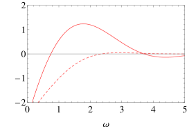
Figure 5: For $\{\alpha=0.7,\,k=-2,\,\beta=1.1\}$, we plot the formal expression for the norm (5.10) with a red dashed line and the left hand side of (4.16), whose zeroes correspond to the allowed frequencies, with a red solid line. Note that the smallest frequency corresponds to a ghost. Exploring the norm numerically for various values of the parameters, we find that this behavior is generic.

Finally, we consider the hybrid boundary conditions. Recall that in section 4.1 we found that there is a pair of complex frequency solutions if the absolute value of the deformation parameter $\kappa$ is large enough. Following the conventions in section 4.1, we denote the critical value by $|\kappa_{c}|$. As mentioned above, these complex frequency solutions correspond to ghost/anti-ghost pairs, so we do not discuss this case any further. Let us now examine the norms of the real frequency solutions. We expect the pair of complex frequency solutions that occur for $|\kappa|>|\kappa_{c}|$ to remain as a ghost/anti-ghost pair when we tune $|\kappa|$ below $|\kappa_{c}|$. We will exhibit ample numerical evidence that this is indeed the case, and thus conclude that ghosts are present for all values of $\kappa$.

Recall that the symplectic structure splits into the contributions from the flat and non-flat sectors as in (3.52), and that the symplectic product is given in terms of the symplectic structure by (3.53). Choosing the Cauchy slice $\Sigma$ on which we evaluate the product to be a surface of constant $t$, we can write the inner product as

$$(A_{1},A_{2})=(A_{1},A_{2})_{nf}+(A_{1},A_{2})_{f}\,,$$ (5.15)

where

$$(A_{1},A_{2})_{nf}={} -i\hat{\alpha}\int_{\Sigma}d^{2}x\Bigl{(}\delta B^{*}_{1\rho}\delta B_{2x}-\delta B^{*}_{1x}\delta B_{2\rho}\Bigr{)}$$ (5.16)

$$(A_{1},A_{2})_{f}={} i\hat{\alpha}\int_{\Sigma}d^{2}x\Bigl{(}\delta_{1}A^{(0)*}_{\rho}\delta_{2}A^{(0)}_{x}-\delta_{1}A^{(0)*}_{x}\delta_{2}A^{(0)}_{\rho}\Bigr{)}.$$ (5.17)

Next, we introduce Fourier decompositions as $\delta B_{\mu}=e^{\frac{i}{L}(-\omega t+kx)}b_{\mu}(k)$, $\delta A^{(0)}_{\mu}=e^{\frac{i}{L}(-\omega t+kx)}a^{(0)}_{\mu}$ and proceed as above by computing (5.16) and (5.17) for generic frequencies $\omega_{1}$ and $\omega_{2}$. The expression (5.16) is then given by (5.8) and it only remains to compute (5.17). We manipulate (5.17) noting that the flatness condition implies that the modes satisfy

$$a^{(0)}_{\rho}=-\frac{i}{k}\left(a^{(0)}_{x}\right)^{\prime}\,,$$ (5.18)

where the prime denotes a radial derivative. Using (5.18) in (5.17) we thus find

$$(A_{1},A_{2})_{f}=\left.-2\pi\hat{\alpha}\,\delta_{k_{1},k_{2}}\,k^{-1}a^{(0)}_{1x}a^{(0)}_{2x}\right|^{\rho=\infty}_{\rho=0}\,.$$ (5.19)

From the regularity condition $a^{(0)}_{x}=0$ at $\rho=0$ we conclude that only the term at $\rho=\infty$ contributes to (5.19). Thus, gathering the results (5.8) and (5.19) we find for generic frequencies

$$(A_{1},A_{2})=2\pi\hat{\alpha}\,e^{it(\omega_{1}-\omega_{2})}\delta_{k_{1},k_{2}}\left[\frac{b^{(+)}_{2u}b^{(-)}_{1v}-b^{(+)}_{1u}b^{(-)}_{2v}}{2(\omega_{1}-\omega_{2})}-\frac{\bigl{(}a^{(0)}_{1u}+a^{(0)}_{1v}\bigr{)}\bigl{(}a^{(0)}_{2u}+a^{(0)}_{2v}\bigr{)}}{4k}\right].$$ (5.20)

We can readily verify that the symplectic structure is conserved by noting that (5.20) vanishes for $\omega_{1}\neq\omega_{2}$ when the boundary conditions (3.22), (3.23), hold. Therefore, the symplectic product can be written in terms of the coefficients of the asymptotic expansion as

$$(A_{1},A_{2})=\pi\hat{\alpha}\,\delta_{\vec{k}_{1},\vec{k}_{2}}\biggl{[}b^{(+)}_{u}\partial_{\omega_{1}}b^{(-)}_{v}-\kappa^{2}\left(\frac{k+\omega}{k-\omega}b^{(+)}_{u}\partial_{\omega_{1}}b^{(+)}_{u}+\frac{2k}{(k-\omega)^{2}}(b^{(+)}_{u})^{2}\right)\biggr{]},$$ (5.21)

where $\omega$ is implicitly given by the solutions of (4.17). Studying (5.21) numerically, we find that there is always a ghost among the lowest real frequency modes that occur for $|\kappa|<|\kappa_{c}|$; see figures 6, 6. Furthermore, we find that this picture continues to hold true for all $|\kappa|$ in the range $0\leq|\kappa|<|\kappa_{c}|$. This must indeed be the case since $\kappa=0$ corresponds to Neumann boundary conditions, which were found above to induce violations of unitarity in the bulk.

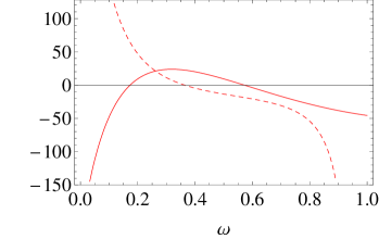
Figure 6: 6: For $\{\alpha=0.8,\,k=1,\,\kappa=0.9\}$ we plot the left hand side of (4.17) (solid line), whose zeros correspond to the allowed frequencies, and the expression for the norm (5.21) (dashed line). We notice that the second to lowest frequency solution is a ghost. By slightly increasing the value of $\kappa$ the solutions move to the complex plane, as seen in figures 3 and 3. 6: For $\{\alpha=0.8$, $k=1$, $\kappa=0.1\}$, we plot the left hand side of (4.17) (solid line) and the expression for the norm (5.21) (dashed line). We observe that the lowest frequency mode found for higher values of $|\kappa|$ disappears, but there is still a ghost in the system.

5.3 Massive sector in Poincaré AdS

We now proceed to compute the symplectic product for the Poincaré AdS modes, focusing on the non-flat piece of the connection. We start with the timelike modes. It should be noted that, since the spectrum is continuous, the products should be understood in the sense of distributions. As usual, in order to evaluate (3.53) we choose $\Sigma$ to be a surface of $t={\rm const}$, so we have

$$(A_{1},A_{2})=i\hat{\alpha}\int dzdx\,\varepsilon^{t\lambda\nu}\delta_{1}B^{*}_{\lambda}\delta_{2}B_{\nu}\,.$$ (5.22)

We find it convenient to use the mode decomposition $\delta B_{\mu}=e^{i(-\omega t+kx)}b_{\mu}(k)$ in (5.22) and computing the integral over $x$ we get

$$(A_{1},A_{2})=2\pi i\hat{\alpha}\,\delta(k_{1}-k_{2})e^{it(\omega_{1}-\omega_{2})}\int_{0}^{\infty}dz\bigl{(}b^{*}_{1z}b_{2x}-b^{*}_{1x}b_{2z}\bigr{)},$$ (5.23)

where we have used $\varepsilon^{ztx}=-1$, in consistency with the convention $\varepsilon^{zuv}=-1$ employed in appendix A.1. It is convenient to express (5.23) in terms of the components $b_{u}$ and $b_{v}$. To this end we note that the first order equation for $b$ implies

$$b_{z}=-\frac{i\alpha}{2kz}(b_{u}-b_{v})-\frac{i}{2k}\left(b_{u}+b_{v}\right)^{\prime}\,,$$ (5.24)

and we recall $b_{x}=\frac{1}{2}(b_{u}+b_{v})$, $b_{t}=\frac{1}{2}(b_{u}-b_{v})$. It follows that we can write

$$i\int_{0}^{\infty}dz(b^{*}_{1z}b_{2x}-b^{*}_{1x}b_{2z})=\frac{\alpha}{2k}\int dz\,z^{-1}\bigl{(}b^{*}_{1v}b_{2v}-b^{*}_{1u}b_{2u}\bigr{)}-\frac{1}{4k}\Bigl{[}\bigl{(}b_{1u}+b_{1v}\bigr{)}^{*}\bigl{(}b_{2u}+b_{2v}\bigr{)}\Bigr{]}\Big{|}_{0}^{\infty}\,.$$ (5.25)

The first two terms in (5.25) correspond to the SL inner product associated to (A.12) and (A.11), respectively. Thus, from the results of appendix B it follows that

$$i\int_{0}^{\infty}dz\bigl{(}b^{*}_{1z}b_{2x}-b^{*}_{1x}b_{2z}\bigr{)}={} \frac{\alpha z^{-1}}{2k(m_{1}^{2}-m_{2}^{2})}\Bigl{[}\bigl{(}b_{1v}b^{\prime}_{2v}-b_{2v}b^{\prime}_{1v}\bigr{)}-\bigl{(}b_{1u}b^{\prime}_{2u}-b_{2u}b^{\prime}_{1u}\bigr{)}\Bigr{]}\Big{|}_{0}^{\infty}$$

$$-\frac{1}{4k}\Bigl{[}\bigl{(}b_{1u}+b_{1v}\bigr{)}^{*}\bigl{(}b_{2u}+b_{2v}\Bigr{)}]\Big{|}_{0}^{\infty}\,,$$ (5.26)

where we have used the explicit form of the SL coefficients (B.4) and (B.5). Next, using the near-boundary expansion one can readily verify that the contribution from $z=0$ to (5.3) vanishes for Dirichlet, Neumann and mixed boundary conditions. The contribution at the Poincaré horizon can be evaluated by introducing a regulator $z_{\infty}$ at large $z$ and using

$$J_{\nu}(x)\to\sqrt{\frac{2}{\pi x}}\cos\left(x-\frac{\nu\pi}{2}-\frac{\pi}{4}\right)\quad\mbox{for }\,\,x\gg 1\,.$$ (5.27)

From this point on the calculation proceeds in close analogy to that for a scalar field in Poincaré AdS. We refer the reader to [26] for details. Up to terms that vanish in the distributional sense, we find that the general expression for the inner product (5.23) reads

$$(A_{1},A_{2})=2\pi\hat{\alpha}\,\delta^{(2)}(k_{1}^{i}-k_{2}^{i}){\cal Q}(\alpha,k)\,,$$ (5.28)

where

$${\cal Q}(\alpha,k_{i})=2\alpha\left|A(\vec{k})+e^{i\pi\alpha}C(\vec{k})\right|^{2}\,.$$ (5.29)

Here we have used that $C$ and $A$ satisfy the relation (4.23). Clearly, the norm (5.28) is manifestly positive definite for Dirichlet, Neumann and mixed boundary conditions.

Let us now calculate the products of the spacelike excitations that are present for mixed boundary conditions. As discussed in section 4.2, their radial profile is given by (A.14) with $C(\vec{k})=0$, which ensures normalizability since they vanish exponentially at the horizon. Furthermore, the mixed boundary condition holds provided the frequencies satisfy (4.27). Recall also that for all $\beta<0$ the spectrum contains a pair of solutions $\psi_{1}$, $\psi_{2}$ whose frequencies are complex conjugate to each other. As argued above, there is always a ghost among these degrees of freedom, so we do not consider this case any further. For $\beta>0$ we found real frequency spacelike solutions, whose norm we now compute.

Since the real frequency spacelike solutions form a discrete set, we compute their norms in analogy to the calculation of the inner product in global coordinates. Our starting point is the general expression (5.3). Because the radial profiles decay exponentially at the horizon, the only non-vanishing contribution to (5.3) comes from the boundary asymptotics. A simple computation reveals that the norm of the real frequency spacelike solutions can be written in terms of the coefficients of the asymptotic expansion as

$$(A_{1},A_{2})_{T}=\pi\hat{\alpha}\,\delta(k_{1}-k_{2})\Bigl{(}b^{(+)}_{u}\partial_{\omega}b^{(-)}_{v}-b^{(-)}_{v}\partial_{\omega}b^{(+)}_{u}\Bigr{)}\,,$$ (5.30)

where $\omega$ satisfies (4.27). Plugging in (5.30) the explicit expressions for the coefficients $b^{(\pm)}$ found previously in (4.25) and (4.26), we find that the norm of the spacelike solution is

$$(A_{1},A_{2})_{T}=\pi\hat{\alpha}\,\delta(k_{1}-k_{2})|A|^{2}\frac{\pi\alpha(k-\alpha\omega)\csc(\pi\alpha)}{p^{2}}\,.$$ (5.31)

Note that the sign of the norm (5.31) is controlled by the factor $(k-\alpha\omega)$. Now, it follows from (4.27) that positive norm solutions occur for positive and negative frequencies, see also figure 4. Thus, we conclude that there are ghosts in the theory for mixed boundary conditions and $\beta>0$.

It only remains to discuss hybrid boundary conditions. In this case, the spectrum consists of both real and imaginary frequencies, regardless of the value of the deformation parameter $\kappa$. As argued above, the existence of non-real frequencies is associated with ghosts on general grounds. Therefore, no detailed calculation of the norms is required to show that this class of theories violate unitarity in the bulk.

As pointed out in [26], bulk theories dual to CFT’s in which the unitarity bound is violated do not necessarily contain ghosts when the geometry is that of Poincaré AdS. Alternatively, the two-point function suffers from a divergence near the light-cone, which implies that the theory does not exist. This motivates us to inspect the near light-cone structure of the Neumann correlators.

The boundary (Wightman) two-point function can be easily computed given the matrix of symplectic products, see e.g. [26]. For the timelike modes in the Neumann theory we find

$$\langle 0|b^{(+)}_{u}(-k_{i})b^{(+)}_{u}(k_{i})|0\rangle=(A_{1},A_{2})^{-1}|_{Neumann}=\frac{4^{\alpha}q^{2}L}{\pi\alpha^{2}\Gamma(-\alpha)^{2}}\frac{(\omega-k)^{1-\alpha}}{(\omega+k)^{1+\alpha}}\,.$$ (5.32)

In order to obtain (5.32) we have normalized the radial profiles such that the leading term is $1$. As expected, the Fourier transform does not converge due to the behavior near $\omega=-k$; this behavior is to be contrasted with the Dirichlet case, in which we find

$$\langle 0|b^{(-)}_{v}(-k_{i})b^{(-)}_{v}(k_{i})|0\rangle=(A_{1},A_{2})^{-1}|_{Dirichlet}=\frac{4^{-\alpha}q^{2}L}{\pi\alpha^{2}\Gamma(\alpha)^{2}}\frac{(\omega+k)^{1+\alpha}}{(\omega-k)^{1-\alpha}}\,.$$ (5.33)

This is clearly finite as we approach $\omega=-k$. In the parameter range of interest, namely $0<\alpha<1$, the divergence near $\omega=k$ is mild enough so that the Fourier transform of (5.33) converges.

The parallel with [26] extends beyond the existence of the light-cone divergence discussed above, in that this divergence can be related to the appearance of lightlike gauge modes. In fact, recall that in section 4.2 we found that the Neumann theory admits the lightlike solution (4.29), which in position space can be written as

$$\delta B=f(u)z^{-\alpha}du\,,$$ (5.34)

where $f$ is an arbitrary function of $u$. From (5.23), it is clear that the aforementioned solution has zero norm since its $z$-component vanishes. Moreover, it is straightforward to verify that the inner product of (5.34) with the timelike modes vanishes in the distributional sense. Thus, assuming that the spectrum of the Neumann theory we found in 4.2 is complete, i.e. that there are only timelike and lightlike modes, we conclude that the lightlike solution (5.34) is a null direction of the symplectic structure and is thus pure gauge. The reader might be somewhat puzzled by the fact that there is a gauge mode which is not flat. However, one can argue that this must be the case by noting the large arbitrariness in (5.34) parametrized by the function $f(u)$, which is unconstrained by the equations of motion.

6 Discussion

By studying the bulk symplectic structure, we have obtained a class of admissible boundary conditions for the MCS system in asymptotically-AdS spaces. According to the holographic dictionary, these boundary conditions determine the operator content in the possible dual theories. In agreement with the existing literature, we find that there is a vector operator of conformal dimension $1\pm\alpha\,$, in addition to the well-known chiral currents which are also present in the pure Chern-Simons theory. The vector operator is associated with the Hodge dual of the bulk field strength, which behaves as a massive vector with a mass proportional to the Chern-Simons coupling. It is worth mentioning that the components of these operators satisfy a constraint, so they have less degrees of freedom than naively expected. This feature is reminiscent of the situation in topologically massive gravity, where similar constraints exist [49]. The chiral currents, on the other hand, are associated to the flat piece of the connection, and are in that sense topological.

Our analysis reveals that, whereas it is possible to impose boundary conditions such that the topological and massive sectors decouple, it is also in principle valid to introduce a mixing between them. In particular, we studied a class of boundary conditions that corresponds to double-trace deformations that couple the chiral currents with the vector operators. Regarding the boundary conditions in which both sectors decouple, we have also considered boundary conditions that yield double-trace deformations within each sector. In this case, it is even possible to generalize these to incorporate multi-trace deformations in the usual way. Our main result is that this apparently large freedom in the choice of boundary conditions is severely restricted once we impose unitarity as an extra requirement.

We have addressed the issue of unitarity by studying the MCS theory both in Poincaré and global AdS. In these setups, the violations of unitarity generically manifest themselves as ghost excitations in the spectrum of the theories defined with given boundary conditions. The boundary conditions that pass the test of unitarity correspond to fixing the leading behavior of the massive sector (Dirichlet boundary conditions), while separately specifying a linear relation between the two components of the flat connection along the boundary directions. It is worth mentioning that the latter also requires a specific choice of sign in the proportionality constant. Furthermore, we mention that for boundary conditions that fix the spatial part of the boundary connection, the topological degrees of freedom become pure gauge (in the absence of holonomies).

For the boundary conditions corresponding to double-trace deformations which involve the massive sector, we contented ourselves with numerical results and the reader may wonder whether our analysis was exhaustive enough to rule out the existence of a non-trivial phase diagram. In particular, since the Dirichlet theory is well defined and we can in principle approach it by continuously tuning the deformation parameters, it is reasonable to ask whether there is an open set of unitarity-preserving values near the Dirichlet point. The answer to this question is negative, as it is most easily seen when the geometry is taken to be the Poincaré patch of $AdS_{3}$. In this case, the presence of a scaling symmetry dictates that, up to sign changes, all non-zero values of the coupling constants are equivalent. One can use this fact to draw conclusions regarding the mixed boundary condition $\delta B^{(+)}_{u}=\beta\,\delta B^{(-)}_{v}$. For the reason we just mentioned, it suffices to study the cases $\beta=0,\,\infty,\,\pm 1$, where $\beta=0$ corresponds to Dirichlet boundary conditions. Then, finding ghosts for $\beta=\pm 1$ implies that these remain for all non-zero $\beta$, forbidding a non-zero critical value. Moreover, noting that the Poincaré patch theory captures the high-momentum dynamics of the theory in global AdS, one can extend this result to the global case. Clearly, the analogous statement holds true for our hybrid boundary conditions parametrized by the constant $\kappa$.

In many scenarios, the presence of the ghosts is in one-to-one correspondence with violations of the unitarity bound in the dual theory, which establishes that the scaling dimension of vector operators must be greater than one. In fact, the operator of dimension $1-\alpha$ violates the bound for all $\alpha$ and, accordingly, we find ghosts whenever the corresponding slow-decaying branch fluctuates. The only exception are the conformally invariant Neumann boundary conditions in the Poincaré patch, which set to zero the faster fall-off. In analogy with the scalar case discussed in [26], we have found in this case that the spectrum is ghost-free, and that the expected pathologies arise instead in the 2-point function, which is ill-defined even at large distances. Interestingly, we also found ghosts in the flat sector, which occur for some choices of the parameter that controls the double-trace deformation. Since the chiral currents have dimension one, these unitarity violations cannot be linked to the bound on the scaling dimension. These pathologies are indeed to be expected, however, because the expression for the symplectic product restricted to the flat sector is not positive definite in any obvious way.

It is worth commenting in more detail on the mixed boundary conditions in relation to the unitarity bound. Above, we obtained these as a deformation of the Neumann theory, as it is customary for bulk scalars whose mass lies in the Breitenlohner-Freedman window. Had the Neumann theory been well defined, the inclusion of the relevant double-trace operator could have been thought of as triggering an RG flow towards the Dirichlet theory. However, as we have seen, the Neumann theory is sick, and inclusion of the double-trace operator does not cure its pathologies. Thus, the aforementioned flow is not well defined. Attempting to remedy this, one might try to understand the mixed boundary conditions as triggering a flow from the Dirichlet theory. In this case, unfortunately, the deformation term one needs to add is of the form $\sim\Bigl{(}B^{(-)}_{v}\Bigr{)}^{2}$, so it corresponds to an irrelevant operator of dimension $2(1+\alpha)$. It follows that the resulting theory is non-renormalizable and the ghosts that arise can be understood as being the result of our loss of control of the theory in the UV.

It is interesting to contrast our results with those of [29], in which the authors found an effective three-dimensional MCS theory in the context of holographic RG flows. More precisely, they constructed five-dimensional solutions in the Einstein-Maxwell-Chern-Simons theory which have the interpretation of magnetic branes. Perturbations around these backgrounds turn out to describe RG flows from four-dimensional field theories in the UV to two-dimensional ones in the IR, and the dynamics of the latter are captured by a 3$d$ MCS theory. Requiring the usual Dirichlet boundary conditions in the UV and imposing matching conditions in the bulk, the effective IR theory contains a double-trace for the vector operators which we denoted by $B^{(\pm)}$. Our analysis reveals that this theory must contain ghosts, and indeed, the results of [29] indicate that violations of unitarity are present if one tries to extend the domain of validity of the IR description to the entire bulk. Then, what saves the theory is the existence of an effective cut-off associated to the domain wall solution, whose presence implies that the IR description breaks down at some intermediate value of the radial coordinate. This is to be expected since Dirichlet boundary conditions were imposed in the UV, and these respect the dual unitarity bounds. The issue of removing the bulk ghosts by introducing the appropriate cut-offs will be discussed in an upcoming publication [50].

We now briefly comment on the implications of our results in the context of potential condensed matter applications. For illustrative purposes, we first review the relevant results of the pure Maxwell theory and then move on to describe how the addition of the Chern-Simons term changes the picture. In terms of the radial variable of (A.17), the asymptotics of the gauge field in the pure Maxwell theory are of the form

$$A_{i}=\log rA^{(1)}_{i}+A^{(0)}_{i}+\ldots\qquad{\rm with}\quad\nabla^{(0)}_{i}A^{(1)i}=0\,,$$ (6.1)

where $i$ is a boundary index and $\nabla^{(0)}$ is the covariant derivative associated with the conformal boundary metric. The conservation equation satisfied by the coefficient $A^{(1)}_{i}$ indicates that it should be interpreted as the $U(1)$ current. This fact was overlooked in [51, 52, 53, 54], in which the authors discussed the construction of a holographic $1+1$ dimensional superfluid/superconductor incorrectly interpreting $A^{(0)}$ as the boundary current. We mention that this confusion was resolved in [27] using the conservation argument given above. However, there is still an obstruction to the study of such holographic theory, since the boundary conditions that allow for a fluctuating current yield ghosts [26]. Thus, the applicability of the by now standard procedure [55, 56] to the study of holographic $1+1$ superconductors remains, at least, unclear. Given this, it is compelling to ask ourselves what are the implications of adding the Chern-Simons term to the Maxwell theory and the possible AdS/CMT applications of the resulting setup. As we have seen, the inclusion of the Chern-Simons term drastically modifies the scenario, as the $U(1)$ vector current is replaced by the topological chiral currents associated to the flat connections, and one can imagine introducing an order parameter (dual to a minimally coupled bulk charged scalar, say) which could potentially break the associated symmetry spontaneously. We leave the exploration of this line of research for future work.

Acknowledgments

We are grateful to Geoffrey Compère, Eduardo Fradkin, Gary Horowitz, Per Kraus, Mukund Rangamani, Simon Ross and Jorge Santos for helpful conversations, and specially to Don Marolf for many useful discussions on these and related topics. T.A. was partly supported by a Fulbright-CONICYT fellowship, by the US National Science Foundation under grant PHY08-55415 and by funds from the University of California. T.A. is also pleased to thank the Department of Physics of the University of Illinois at Urbana-Champaign and the Department of Mathematics of the University of California, Davis, for their hospitality during the completion of this work. RGL is partially supported by the US Department of Energy under contract FG02-91-ER40709. The work of J.I.J. is supported by the research programme of the Foundation for Fundamental Research on Matter (FOM), which is part of the Netherlands Organisation for Scientific Research (NWO).

Appendix A Solutions to the equations of motion on $AdS_{3}$

Here we consider the MCS equation (2.2) on a fixed background geometry. We remark that since the MCS system is linear, in the probe approximation both the background gauge field and its fluctuations satisfy the same equation. Splitting the gauge field fluctuation as in (2.6), i.e. $\delta A=\delta B+\delta A^{(0)}$, we have that $\delta A^{(0)}$ is flat and $\delta B$ satisfies

$$0=\epsilon^{\mu\nu\rho}\partial_{\nu}\delta B_{\rho}+\frac{\alpha}{L}\delta B^{\mu}\,,$$ (A.1)

where $\epsilon^{\mu\nu\rho}=-1/\sqrt{|g|}\varepsilon^{\mu\nu\rho}$ and $g$ is the determinant of the background metric. In what follows we present the general solution of this equation for the backgrounds of interest, namely $AdS_{3}$ in both the Poincaré patch and global coordinates.

A.1 Poincaré patch of $AdS_{3}$

We first consider the background geometry to be the Poincaré patch of $AdS_{3}\,$, with line element given by

$$ds^{2}=\frac{L^{2}}{z^{2}}\left(dz^{2}-dt^{2}+dx^{2}\right).$$ (A.2)

We remind the reader that the line element (A.2) posses the symmetry

$$z\rightarrow\lambda z\,,\qquad t\rightarrow\lambda t\,,\qquad x\rightarrow\lambda x\,,$$ (A.3)

which corresponds to dilations in the dual theory. This symmetry play an important role in the analysis of the spectrum, as discussed in the main text. It will prove convenient to introduce null coordinates

$$t=u-v\,,\quad x=u+v\,,$$ (A.4)

so that the line element reads

$$ds^{2}=\frac{L^{2}}{z^{2}}\left(dz^{2}+4dudv\right).$$ (A.5)

By convention, we take $\varepsilon^{zuv}=-1$. We Fourier-decompose the fluctuations of the gauge-invariant (massive) mode as

$$\delta B_{\mu}(u,v;z)=e^{i(k_{u}u+k_{v}v)}b_{\mu}(z),$$ (A.6)

where $k_{u}=k-\omega$ and $k_{v}=k+\omega$. Inserting (A.5) and (A.6) in (A.1) we find

$$0={} 2\alpha\,b_{z}+iz\bigl{(}k_{u}b_{v}-k_{v}b_{u}\bigr{)}\,,$$ (A.7)

$$0={} \alpha\,b_{v}+z\bigl{(}ik_{v}b_{z}-b_{v}^{\prime}\bigr{)}\,,$$ (A.8)

$$0={} \alpha\,b_{u}+z\bigl{(}-ik_{u}b_{z}+b_{u}^{\prime}\bigr{)}\,.$$ (A.9)

The above equations can be decoupled by going to second order in derivatives, obtaining

$$0={} z^{2}b^{\prime\prime}_{z}-zb^{\prime}_{z}-\bigl{[}\alpha^{2}-1-m^{2}z^{2}\bigr{]}b_{z}\,,$$ (A.10)

$$0={} z^{2}b^{\prime\prime}_{u}-zb^{\prime}_{u}-\bigl{[}\alpha(\alpha+2)-m^{2}z^{2}\bigr{]}b_{u}\,,$$ (A.11)

$$0={} z^{2}b^{\prime\prime}_{v}-zb^{\prime}_{v}-\bigl{[}\alpha(\alpha-2)-m^{2}z^{2}\bigr{]}b_{v}\,,$$ (A.12)

where $m^{2}\equiv-k_{u}k_{v}=\omega^{2}-k^{2}$ is the eigenvalue of the Laplacian associated to the conformal boundary metric. Once the general solution to the second order equations has been found, the first order equations provide relations among the various integration constants.

A.1.1 Timelike modes ($m^{2}>0$)

For timelike momenta and $\alpha\notin\mathds{Z}$ we can write the general solution of (A.7)-(A.12) as

$$b_{z}={} imz\left[A(\vec{k})J_{\alpha}(mz)+C(\vec{k})J_{-\alpha}(mz)\right]$$

$$b_{u}={} k_{u}z\left[-A(\vec{k})J_{1+\alpha}(mz)+C(\vec{k})J_{-1-\alpha}(mz)\right]$$ (A.13)

$$b_{v}={} k_{v}z\left[A(\vec{k})J_{-1+\alpha}(mz)-C(\vec{k})J_{1-\alpha}(mz)\right],$$

where $J_{\nu}$ is the Bessel function of the first kind.

A.1.2 Spacelike modes $(m^{2}<0)$

In this case we define $m^{2}\equiv-p^{2}$, so that $p^{2}>0$. The general solution is then

$$b_{z}={} ipz\left[A(\vec{k})K_{\alpha}(pz)+C(\vec{k})I_{\alpha}(pz)\right]$$

$$b_{u}={} k_{u}z\left[A(\vec{k})K_{1+\alpha}(pz)-C(\vec{k})I_{1+\alpha}(pz)\right]$$ (A.14)

$$b_{v}={} k_{v}z\left[A(\vec{k})K_{-1+\alpha}(pz)-C(\vec{k})I_{-1+\alpha}(pz)\right],$$

where $I_{\nu}$ and $K_{\nu}$ are the modified Bessel functions of the first and second kind, respectively.

A.1.3 Lightlike modes ($m^{2}=0$)

• Right-moving ($k_{v}=0$):

  $$b_{z}=-C\,\frac{ik_{u}}{2\alpha}z^{1+\alpha}\,,\qquad b_{u}=Az^{-\alpha}+C\,\frac{k_{u}^{2}}{4\alpha(1+\alpha)}z^{2+\alpha}\,,\qquad b_{v}=C\,z^{\alpha}\,.$$ (A.15)

• Left-moving ($k_{u}=0$):

  $$b_{z}=A\,\frac{ik_{v}}{2\alpha}z^{1-\alpha}\,,\qquad b_{u}=A\,z^{-\alpha}\,,\qquad b_{v}=A\,\frac{k_{v}^{2}}{4\alpha(\alpha-1)}z^{2-\alpha}+Cz^{\alpha}\,.$$ (A.16)

A.2 Global $AdS_{3}$

We now consider the global $AdS_{3}$ metric written as

$$ds^{2}=\frac{dr^{2}}{1+\displaystyle{\frac{r^{2}}{L^{2}}}}-\left(1+\frac{r^{2}}{L^{2}}\right)dt^{2}+\frac{r^{2}}{L^{2}}dx^{2}\,,$$ (A.17)

where we have defined $x\equiv L\varphi$. We will use the dimensionless radial coordinate $\rho=r/L$, so we write

$$\delta B=e^{\frac{i}{L}\left(-\omega t+kx\right)}\Bigl{[}L\,b_{\rho}(\rho)\,d\rho+b_{t}(\rho)\,dt+b_{x}(\rho)\,dx\Bigr{]}.$$ (A.18)

Single-valuedness of the solution demands that we identify $x\sim x+2\pi L$, so the dimensionless momentum $k$ is an integer, $k\in\mathds{Z}$. Following the same steps as before to decouple the equations we find

$$0={} \rho^{2}\left(1+\rho^{2}\right)b_{u}^{\prime\prime}+\rho\left(1+3\rho^{2}\right)b_{u}^{\prime}+\left(\frac{\rho^{2}}{1+\rho^{2}}\omega^{2}-\alpha(\alpha+2)\rho^{2}-k^{2}\right)b_{u}$$ (A.19)

$$0={} \rho^{2}\left(1+\rho^{2}\right)b_{v}^{\prime\prime}+\rho\left(1+3\rho^{2}\right)b_{v}^{\prime}+\left(\frac{\rho^{2}}{1+\rho^{2}}\omega^{2}-\alpha(\alpha-2)\rho^{2}-k^{2}\right)b_{v}\,,$$ (A.20)

where $b_{v}=b_{x}-b_{t}$ and $b_{u}=b_{t}+b_{x}$ as before. Notice that the equations are related by $\alpha\leftrightarrow-\alpha$. When $k\neq 0$, their solution is

$$b_{u}={} C_{u}^{(+)}F(\omega,k,\alpha;\rho)+C_{u}^{(-)}F(\omega,-k,\alpha;\rho)$$ (A.21)

$$b_{v}={} C_{v}^{(+)}F(\omega,k,-\alpha;\rho)+C_{v}^{(-)}F(\omega,-k,-\alpha;\rho)$$ (A.22)

with

$$F(\omega,k,\alpha;\rho)=\rho^{k}(1+\rho^{2})^{\omega/2}\,_{2}F_{1}\left(\frac{1}{2}(k-\alpha+\omega),\frac{1}{2}(2+k+\alpha+\omega);1+k;-\rho^{2}\right),$$ (A.23)

where ${}_{2}F_{1}$ is the Gauss Hypergeometric function. We can obtain $b_{\rho}$ from the $\rho$ component of (2.8), which reads

$$0={} \alpha\,b_{\rho}+\frac{i}{\rho(1+\rho^{2})}\left(\omega b_{x}+kb_{t}\right)$$

$$={} \alpha\,b_{\rho}+\frac{i}{2\rho(1+\rho^{2})}\Bigl{[}\left(k+\omega\right)b_{u}+\left(\omega-k\right)b_{v}\Bigr{]}.$$ (A.24)

Finally, inserting our solution back into the first order equation (2.8) we find the relations

$$C_{v}^{(+)}={} \frac{k-\alpha+\omega}{k+\alpha-\omega}C_{u}^{(+)}$$ (A.25)

$$C_{v}^{(-)}={} \frac{k+\alpha+\omega}{k-\alpha-\omega}C_{u}^{(-)}\,,$$ (A.26)

so there are only two independent degrees of freedom.

When $k=0$, the basis of solutions (A.21) is no longer valid. Instead, one can use

$$b_{u}={} (1+\rho^{2})^{\omega/2}\left[\tilde{C}_{u}^{(+)}\tilde{F}_{1}(\omega,\alpha;\rho)+\tilde{C}_{u}^{(-)}\tilde{F}_{2}(\omega,\alpha;\rho)\right]$$ (A.27)

$$b_{v}={} (1+\rho^{2})^{\omega/2}\left[\tilde{C}_{u}^{(+)}\tilde{F}_{1}(\omega,-\alpha;\rho)+\tilde{C}_{u}^{(-)}\tilde{F}_{2}(\omega,-\alpha;\rho)\right],$$ (A.28)

where

$$\tilde{F}_{1}(\omega,\alpha;\rho)={} \,{}_{2}F_{1}\left(a,b;1;-\rho^{2}\right),$$ (A.29)

$$\tilde{F}_{2}(\omega,\alpha;\rho)={} {}_{2}F_{1}\left(a,b;1;-\rho^{2}\right)\log(-\rho^{2})$$

$$+\sum_{n=1}^{\infty} \frac{(a)_{n}(b)_{n}}{(n!)^{2}}(-\rho^{2})^{n}\Bigl{[}\psi(a+n)-\psi(a)+\psi(b+n)-\psi(b)-2\psi(n+1)+2\psi(1)\Bigr{]}.$$ (A.30)

Here $a=(\omega-\alpha)/2$ , $b=(2+\alpha+\omega)/2$ and $(a)_{n}$ is the Pochhammer symbol defined by $(a)_{n}=\Gamma(a+n)/\Gamma(a)$. The presence of the logarithm in (A.2) makes the solution non-normalizable at the origin. Therefore, we set $\tilde{C}_{u}^{(-)}=\tilde{C}_{u}^{(-)}=0\,$, and will not consider the profile (A.2) in the body of the paper. Once again, $b_{\rho}$ can be obtained using (A.24). The full solution is then obtained noting that the first order equations require

$$\tilde{C}_{v}^{(+)}=-\tilde{C}_{u}^{(+)}\,.$$ (A.31)

Appendix B Sturm-Liouville problem

The Sturm-Liouville eigenvalue problem in the interval $x\in(a,b)$ is characterized by the second order ODE

$$L\psi=\lambda\psi\,,\qquad{\rm where}\quad L=\frac{1}{w(x)}\left[-\frac{d}{dx}\left(p(x)\frac{d}{dx}\right)+q(x)\right].$$ (B.1)

For given boundary conditions at $x=a$ and $x=b$, the solution of the problem corresponds to a given set of eigenfunctions $\psi_{\lambda}$ with eigenvalue $\lambda$. We can define an associated inner product as

$$\langle\psi_{1},\psi_{2}\rangle=\int_{a}^{b}dx\,w(x)\psi_{1}^{*}\psi_{2}\,.$$ (B.2)

If the boundary conditions are such that the operator $L$ is self-adjoint, it follows that the eigenvalues are real. In addition, eigenfunctions with different eigenvalue are orthogonal with respect to (B.2). Moreover, integrating by parts in the expression $\langle L\psi_{1},\psi_{2}\rangle$ one can show

$$\langle\psi_{1},\psi_{2}\rangle=\frac{p(x)}{\lambda_{1}-\lambda_{2}}\left[\psi_{1}^{*}\frac{d}{dx}\psi_{2}-\psi_{2}\frac{d}{dx}\psi_{1}^{*}\right]\bigg{|}_{a}^{b}\,\,,$$ (B.3)

which reduces the calculation of the integral in the l.h.s. to a simple expression that only involves the asymptotics of $\psi$. In order to apply (B.3) to the computation of symplectic products, we write the integrals of interest in terms of variables which satisfy decoupled equations of the form (B.1) for some $\lambda$, $p$, $w$, $q$. In particular, we note that (A.11) adopts the SL form with $\lambda=m^{2}$ and

$$p=z^{-1}\,,\qquad w=z^{-1}\,,\qquad q=\alpha(\alpha+2)z^{-3}\,,$$ (B.4)

while for (A.12) we have $\lambda=m^{2}$ in addition to

$$p=z^{-1}\,,\qquad w=z^{-1}\,,\qquad q=\alpha(\alpha-2)z^{-3}\,.$$ (B.5)

Similarly, equation (A.19) can be written as a SL problem with $\lambda=\omega^{2}$ and

$$p=\rho(1+\rho^{2})\,,\qquad w=\frac{\rho}{1+\rho^{2}}\,,\qquad q=\frac{k^{2}}{\rho}+\alpha(\alpha+2)\rho\,,$$ (B.6)

while for (A.20) we have $\lambda=\omega^{2}$ and

$$p=\rho(1+\rho^{2})\,,\qquad w=\frac{\rho}{1+\rho^{2}}\,,\qquad q=\frac{k^{2}}{\rho}+\alpha(\alpha-2)\rho\,.$$ (B.7)

Appendix C $U(1)$ symmetries

The goal of this appendix is to study the character of the $U(1)$ transformations from the point of view of possible boundary field theory duals. We recall that these transformations act on the fields as

$$\delta_{\lambda}A_{\mu}=\partial_{\mu}\lambda\,,$$ (C.1)

where $\lambda$ is a single-valued arbitrary function of spacetime. By considering only single-valued functions we are ruling out “large” gauge transformations, which are not connected with the identity. Our approach will be to note that symmetries of the bulk theory that have a non-trivial action on the boundary data (i.e. the boundary sources and operators) are naturally interpreted as symmetries of the boundary theory. Our analysis follows that of [57, 58, 43] regarding boundary diffeomorphisms. For the sake of concreteness, we shall assume in this section that the background geometry is global AdS. Analogous results apply to the Poincaré case.

Quite generally, a symmetry is a transformation that preserves the phase space of the theory. As a consequence, it follows that such a transformation must leave both the action and the boundary conditions invariant. From the boundary point of view, this ensures that the quantum generating functional is invariant under the symmetry of interest. Obviously, the $U(1)$ is a symmetry of the equations of motion (2.2). However, if this transformation acts non-trivially on the boundary, it may or may not preserve the boundary conditions and the action functional. In fact, depending on the boundary conditions, the $U(1)$ transformation could be a global symmetry, a gauge symmetry or might not even be a symmetry at all. By a gauge symmetry we mean a transformation whose generator (i.e. the associated charge) vanishes on shell. Global symmetries, on the other hand, have non-zero charge. It should be noted that this charge ought to be integrable and finite for the corresponding transformation to be properly implemented in phase space.

Let us first establish the fact that the $U(1)$ symmetries that act trivially on the boundary are pure gauge (in the sense that they are null directions of $\Omega$). First, we note that these are in fact symmetries since they leave both the action and the boundary conditions invariant. Furthermore, by a calculation identical to the one in section 5.1, we conclude that the symplectic product of $\delta_{\lambda}A=\nabla\lambda$ with an arbitrary configuration $\delta A$ is given by

$$\Omega(\delta_{\lambda}A,\delta A)=\hat{\alpha}\int_{\partial\Sigma}dx\,\lambda\,\delta A^{(0)}_{x}\,,$$ (C.2)

where $\delta A^{(0)}_{x}$ is the flat piece of $\delta A$ and $\partial\Sigma$ corresponds to the intersection of the boundary with a $t={\rm const.}$ slice. Comparing (C.2) with (3.2), we conclude that the $U(1)$ transformations that leave the boundary invariant have vanishing charge and are thus pure gauge. As mentioned above, since these transformations leave the boundary data invariant, they do not manifest in the dual theory.

We now consider transformations whose action on the boundary data is non-trivial, and examine their action on the various boundary conditions under consideration. We begin with hybrid boundary conditions. Since these mix the flat connections with the massive sector, and the $U(1)$ acts only on the former, it is clear that the $U(1)$ transformations are not symmetries of the theory. Let us now focus on boundary conditions which do not mix the flat and massive sectors. Since the $U(1)$ transformations only affect the flat piece of the connection, we concentrate our attention in the flat sector. It follows from (C.2) that theories in which $A_{x}^{(0)}$ is fixed have the residual gauge symmetry associated with $\lambda|_{\partial M}=\lambda(t)$. Since this acts non-trivially at the boundary, we conclude that the gauge symmetry is also present in the dual theory. Consider now the boundary condition $\delta A^{(0)}_{t}=0$, in which case the residual symmetry corresponds to $\lambda|_{\partial M}=\lambda(x)$. We see from (C.2) that there is an associated non-vanishing infinitesimal charge, given by the right hand side of (C.2) (see section 3, in particular eq. (3.2)). We notice that (C.2) is trivially integrable, so we can write an expression for the total charge as

$$Q_{\lambda}=\hat{\alpha}\int_{\partial\Sigma}dx\,\lambda(x)A^{(0)}_{x}\,.$$ (C.3)

The existence of the well-defined non-vanishing charge (C.3) implies that the associated symmetry is global. Once again, this transformation acts non-trivially on the boundary so it is present in the boundary theory. It is worth emphasizing that the aforementioned symmetry is in fact infinite dimensional, and that the charges (C.3) correspond to the chiral currents discussed previously in the literature. This can be seen by computing the Poisson bracket $\{Q_{\lambda},Q_{\sigma}\}$. The easiest way to proceed is to note that the charges are the generators of the associated symmetry, so it must be the case that

$$\{Q_{\lambda},Q_{\sigma}\}=\delta_{\sigma}Q_{\lambda}\,,$$ (C.4)

where $\delta_{\sigma}$ is an infinitesimal $U(1)$ transformation with parameter $\sigma$. Using the explicit expression for $Q_{\lambda}$ in (C.3), we can compute the variation of the right hand side in (C.4) and conclude

$$\{Q_{\lambda},Q_{\sigma}\}=\hat{\alpha}\int_{\partial\Sigma}dx\,\lambda(x)\partial_{x}\sigma(x)\,,$$ (C.5)

which is the algebra of the chiral currents. By a calculation similar to the one above, we can show that analogous global symmetries are present in theories defined with the boundary condition (4.2) with finite $\hat{\beta}$.

References

- [1] J. M. Maldacena, “The Large N limit of superconformal field theories and supergravity,” Adv.Theor.Math.Phys. 2 (1998) 231–252, arXiv:hep-th/9711200 [hep-th].
- [2] E. Witten, “Anti-de Sitter space and holography,” Adv. Theor. Math. Phys. 2 (1998) 253–291, arXiv:hep-th/9802150.
- [3] S. Gubser, I. R. Klebanov, and A. M. Polyakov, “Gauge theory correlators from noncritical string theory,” Phys.Lett. B428 (1998) 105–114, arXiv:hep-th/9802109 [hep-th].
- [4] J. D. Brown and M. Henneaux, “Central Charges in the Canonical Realization of Asymptotic Symmetries: An Example from Three-Dimensional Gravity,” Commun. Math. Phys. 104 (1986) 207–226.
- [5] D. Birmingham, I. Sachs, and S. N. Solodukhin, “Conformal field theory interpretation of black hole quasi- normal modes,” Phys. Rev. Lett. 88 (2002) 151301, arXiv:hep-th/0112055.
- [6] S. Deser, R. Jackiw, and S. Templeton, “Topologically massive gauge theories,” Ann. Phys. 140 (1982) 372–411.
- [7] S. Deser, R. Jackiw, and S. Templeton, “Three-Dimensional Massive Gauge Theories,” Phys. Rev. Lett. 48 (1982) 975–978.
- [8] P. Kraus and F. Larsen, “Partition functions and elliptic genera from supergravity,” JHEP 01 (2007) 002, arXiv:hep-th/0607138.
- [9] P. Kraus, “Lectures on black holes and the AdS(3)/CFT(2) correspondence,” Lect. Notes Phys. 755 (2008) 193–247, arXiv:hep-th/0609074.
- [10] X. G. Wen, “Gapless boundary excitations in the quantum Hall states and in the chiral spin states,” Phys. Rev. B43 (1991) 11025–11036.
- [11] E. Witten, “Quantum field theory and the Jones polynomial,” Commun. Math. Phys. 121 (1989) 351.
- [12] G. W. Moore and N. Seiberg, “Taming the Conformal Zoo,” Phys. Lett. B220 (1989) 422.
- [13] S. Elitzur, G. W. Moore, A. Schwimmer, and N. Seiberg, “Remarks on the Canonical Quantization of the Chern-Simons- Witten Theory,” Nucl. Phys. B326 (1989) 108.
- [14] A. P. Balachandran, G. Bimonte, K. S. Gupta, and A. Stern, “Conformal edge currents in Chern-Simons theories,” Int. J. Mod. Phys. A7 (1992) 4655–4670, arXiv:hep-th/9110072.
- [15] M. Bos and V. Nair, “Coherent State Quantization of Chern-Simons Theory,” Int.J.Mod.Phys. A5 (1990) 959.
- [16] M. Bos and V. Nair, “U(1) Chern-Simons Theory and c=1 Conformal Blocks,” Phys.Lett. B223 (1989) 61.
- [17] A. S. Schwarz, “The Partition Function of a Degenerate Functional,” Commun.Math.Phys. 67 (1979) 1–16.
- [18] S. Gukov, E. Martinec, G. W. Moore, and A. Strominger, “Chern-Simons gauge theory and the AdS(3)/CFT(2) correspondence,” arXiv:hep-th/0403225.
- [19] D. Marolf and S. F. Ross, “Boundary conditions and new dualities: Vector fields in AdS/CFT,” JHEP 11 (2006) 085, arXiv:hep-th/0606113.
- [20] A. J. Amsel and D. Marolf, “Energy bounds in designer gravity,” Phys. Rev. D74 (2006) 064006, arXiv:hep-th/0605101.
- [21] A. J. Amsel and D. Marolf, “Supersymmetric Multi-trace Boundary Conditions in AdS,” Class.Quant.Grav. 26 (2009) 025010, arXiv:0808.2184 [hep-th].
- [22] G. Mack, “All Unitary Ray Representations of the Conformal Group SU(2,2) with Positive Energy,” Commun.Math.Phys. 55 (1977) 1.
- [23] S. Minwalla, “Restrictions imposed by superconformal invariance on quantum field theories,” Adv.Theor.Math.Phys. 2 (1998) 781–846, arXiv:hep-th/9712074 [hep-th].
- [24] V. Balasubramanian, P. Kraus, and A. E. Lawrence, “Bulk vs. boundary dynamics in anti-de Sitter spacetime,” Phys. Rev. D59 (1999) 046003, arXiv:hep-th/9805171.
- [25] E. Witten, “Multi-trace operators, boundary conditions, and AdS/CFT correspondence,” arXiv:hep-th/0112258.
- [26] T. Andrade and D. Marolf, “AdS/CFT beyond the unitarity bound,” JHEP 1201 (2012) 049, arXiv:1105.6337 [hep-th].
- [27] K. Jensen, “Chiral anomalies and AdS/CMT in two dimensions,” JHEP 01 (2011) 109, arXiv:1012.4831 [hep-th].
- [28] P. Minces and V. O. Rivelles, “Chern-Simons theories in the AdS / CFT correspondence,” Phys.Lett. B455 (1999) 147–154, arXiv:hep-th/9902123 [hep-th].
- [29] E. D’Hoker, P. Kraus, and A. Shah, “RG Flow of Magnetic Brane Correlators,” JHEP 04 (2011) 039, arXiv:1012.5072 [hep-th].
- [30] H.-U. Yee and I. Zahed, “Holographic two dimensional QCD and Chern-Simons term,” arXiv:1103.6286 [hep-th].
- [31] S. Carlip, S. Deser, A. Waldron, and D. K. Wise, “Cosmological Topologically Massive Gravitons and Photons,” Class. Quant. Grav. 26 (2009) 075008, arXiv:0803.3998 [hep-th].
- [32] M. Fujita, W. Li, S. Ryu, and T. Takayanagi, “Fractional Quantum Hall Effect via Holography: Chern-Simons, Edge States, and Hierarchy,” JHEP 0906 (2009) 066, arXiv:0901.0924 [hep-th].
- [33] V. Balasubramanian, I. Garcia-Etxebarria, F. Larsen, and J. Simon, “Helical Luttinger Liquids and Three Dimensional Black Holes,” arXiv:1012.4363 [hep-th].
- [34] C. D. Fosco, E. F. Moreno, and F. A. Schaposnik, “Fermions in an AdS3 Black Hole Background and the Gauge- Gravity Duality,” arXiv:1109.0491 [hep-th].
- [35] K. Skenderis, “Lecture notes on holographic renormalization,” Class. Quant. Grav. 19 (2002) 5849–5876, arXiv:hep-th/0209067.
- [36] S. El-Showk, Y. Nakayama, and S. Rychkov, “What Maxwell Theory in D¡¿4 teaches us about scale and conformal invariance,” Nucl. Phys. B848 (2011) 578–593, arXiv:1101.5385 [hep-th].
- [37] J. Lee and R. M. Wald, “Local symmetries and constraints,” J.Math.Phys. 31 (1990) 725–743.
- [38] R. M. Wald, “Quantum field theory in curved space-time and black hole thermodynamics,”. Chicago, USA: Univ. Pr. (1994) 205 p.
- [39] R. M. Wald and A. Zoupas, “A General definition of ’conserved quantities’ in general relativity and other theories of gravity,” Phys.Rev. D61 (2000) 084027, arXiv:gr-qc/9911095 [gr-qc].
- [40] V. Iyer and R. M. Wald, “Some properties of Noether charge and a proposal for dynamical black hole entropy,” Phys. Rev. D50 (1994) 846–864, arXiv:gr-qc/9403028.
- [41] A. Ashtekar, L. Bombelli, and O. Reula, “The Covariant Phase Space of Asymptotically Flat Gravitational Fields,”. Print-90-0318 (SYRACUSE).
- [42] R. M. Wald, “Black hole entropy is the Noether charge,” Phys. Rev. D48 (1993) 3427–3431, arXiv:gr-qc/9307038.
- [43] G. Compere and D. Marolf, “Setting the boundary free in AdS/CFT,” Class.Quant.Grav. 25 (2008) 195014, arXiv:0805.1902 [hep-th].
- [44] M. Berkooz, A. Sever, and A. Shomer, “Double-trace deformations, boundary conditions and spacetime singularities,” JHEP 05 (2002) 034, arXiv:hep-th/0112264.
- [45] S. S. Gubser and I. Mitra, “Double-trace operators and one-loop vacuum energy in AdS/CFT,” Phys. Rev. D67 (2003) 064018, arXiv:hep-th/0210093.
- [46] S. S. Gubser and I. R. Klebanov, “A universal result on central charges in the presence of double-trace deformations,” Nucl. Phys. B656 (2003) 23–36, arXiv:hep-th/0212138.
- [47] R. G. Leigh and A. C. Petkou, “Holography of the N=1 higher spin theory on AdS(4),” JHEP 0306 (2003) 011, arXiv:hep-th/0304217 [hep-th].
- [48] T. Hartman and L. Rastelli, “Double-trace deformations, mixed boundary conditions and functional determinants in AdS/CFT,” JHEP 01 (2008) 019, arXiv:hep-th/0602106.
- [49] K. Skenderis, M. Taylor, and B. C. van Rees, “Topologically Massive Gravity and the AdS/CFT Correspondence,” JHEP 0909 (2009) 045, arXiv:0906.4926 [hep-th].
- [50] T. Andrade, T. Faulkner, and D. Marolf, to appear .
- [51] J. Ren, “One-dimensional holographic superconductor from AdS3/CFT2 correspondence,” JHEP 11 (2010) 055, arXiv:1008.3904 [hep-th].
- [52] A. J. Nurmagambetov, “Analytical approach to phase transitions in rotating and non-rotating 2D holographic superconductors,” arXiv:1107.2909 [hep-th].
- [53] Y. Liu, Q. Pan, and B. Wang, “Holographic superconductor developed in BTZ black hole background with backreactions,” Phys. Lett. B702 (2011) 94–99, arXiv:1106.4353 [hep-th].
- [54] N. Lashkari, “Holographic Symmetry-Breaking Phases in AdS3/CFT2,” arXiv:1011.3520 [hep-th].
- [55] S. A. Hartnoll, C. P. Herzog, and G. T. Horowitz, “Building a Holographic Superconductor,” Phys. Rev. Lett. 101 (2008) 031601, arXiv:0803.3295 [hep-th].
- [56] S. A. Hartnoll, C. P. Herzog, and G. T. Horowitz, “Holographic Superconductors,” JHEP 12 (2008) 015, arXiv:0810.1563 [hep-th].
- [57] G. Barnich and F. Brandt, “Covariant theory of asymptotic symmetries, conservation laws and central charges,” Nucl.Phys. B633 (2002) 3–82, arXiv:hep-th/0111246 [hep-th].
- [58] G. Barnich and G. Compere, “Surface charge algebra in gauge theories and thermodynamic integrability,” J.Math.Phys. 49 (2008) 042901, arXiv:0708.2378 [gr-qc].