Implicit–explicit timestepping with finite element approximation of reaction–diffusion systems on evolving domains

Abstract.

We present and analyse an implicit–explicit timestepping procedure with finite element spatial approximation for a semilinear reaction–diffusion systems on evolving domains arising from biological models, such as Schnakenberg’s (1979). We employ a Lagrangian formulation of the model equations which permits the error analysis for parabolic equations on a fixed domain but introduces technical difficulties, foremost the space-time dependent conductivity and diffusion. We prove optimal-order error estimates in the $\operatorname{L}_{\infty}(0,T;\operatorname{L}_{2}(\varOmega))$ and $\operatorname{L}_{2}(0,T;\operatorname{H}^{1}(\varOmega))$ norms, and a pointwise stability result. We remark that these apply to Eulerian solutions. Details on the implementation of the Lagrangian and the Eulerian scheme are provided. We also report on a numerical experiment for an application to pattern formation on an evolving domain.

1. Introduction

Since the seminal paper of Turing [43], time-dependent reaction–diffusion systems (RDSs) have been studied as models for pattern formation in natural-process driven morphogenesis and developmental biology (see Murray [34] for details). An important generalisation of these models consists in considering RDSs posed on evolving domains. This stems from the now relatively well-known observation that in many cases growth of organisms plays a pivotal role in the emergence of patterns and their evolution during growth development [34, 23]. RDSs on evolving domains have a wider scope of application, e.g., competing-species of micro-organisms in environmental biology, chemistry of materials and corrosion processes, the spread of pollutants. Numerical simulations of RDSs on time-evolving domains reproducing the empirically observed pattern formation processes are commonly used [23, 5, 32, 4, 44, 14]. It is essential for scientists to computationally approximate and appreciate the error between simulations and exact solutions of such RDSs. Galerkin finite elements [41] are among the methods of choice to approximate such systems.

In spite of their widespread use, to the best of our knowledge, no complete error analysis of approximating finite element schemes for nonlinear reaction–diffusion systems on evolving domains is available in the literature, thus motivating this work. This is a sibling paper to [45] where we analysed the well-posed nature of (exact) RDSs on evolving domains. In most practical applications, the evolving domain is usually a surface embedded in the three-dimensional Euclidean space, but for simplicity we restrict our discussion to the case where both the reference domain and the evolving domain are flat, deferring thus the analysis of RDSs on evolving curved surfaces.

1.1. Problem (RDS on a time-dependent evolving domain)

We study a RDS, also considered in [10, 27], which models a system of chemicals that interact through the reaction terms only and diffuse in the domain independently of each other. Given an integer $m\geq 1$, the vector $\boldsymbol{u}\left(\boldsymbol{x},t\right)\in\mathbb{R}^{m}$, denoting the concentration of the chemical species $i=1,\dotsc,m$, at a spatial point $\boldsymbol{x}\in{\Omega_{t}}\subset\mathbb{R}^{d}$, $d=1,2,3$, at time $t\in[0,T]$, $T>0$, satisfies the following initial–boundary value problem

(1.1) $$\begin{gathered}\partial_{t}{u}_{i}(\boldsymbol{x},t)-D_{i}\Updelta{u}_{i}(\boldsymbol{x},t)+\nabla\cdot\left[\boldsymbol{a}u_{i}\right](\boldsymbol{x},t)=f_{i}\left(\boldsymbol{u}(\boldsymbol{x},t)\right),\quad\boldsymbol{x}\in{\Omega_{t}},t\in(0,T],\\ [{\boldsymbol{\nu}}\cdot\nabla{u}_{i}](\boldsymbol{x},t)=0,\quad\boldsymbol{x}\in\partial{\Omega_{t}},t>0,\\ u_{i}(\boldsymbol{x},0)=u_{i}^{0}(\boldsymbol{x}),\quad\boldsymbol{x}\in{\Omega}_{0},\end{gathered}$$

where $\Omega_{t}$, detailed in §2.2, is a simply connected Lipschitz continuously evolving domain with respect to $t\in[0,T]$, and $\boldsymbol{D}\mathrel{\mathop{\mathchar 58\relax}}=({D}_{1},\dotsc,{D}_{m})^{\mathsf{T}}$ is a vector of strictly positive diffusion coefficients. Detailed assumptions on the nonlinear reaction vector field $\boldsymbol{f}\mathrel{\mathop{\mathchar 58\relax}}=({f}_{1},\dotsc,{f}_{m})^{\mathsf{T}}$ are given in §2.5. The convection $\boldsymbol{a}=(a_{1},\dotsc,a_{d})^{\mathsf{T}}$ is induced by the material deformation due to the evolution of the domain. The initial data $\boldsymbol{u}^{0}$ is a positive-entry bounded field. Since we are primarily interested in pattern formation phenomena that arise as a result of self-organisation within a domain without outside-world communication we consider homogeneous Neumann boundary conditions, but other types of boundary conditions could be studied as well within our framework.

1.2. Main results

The core result in this paper is Theorem 5.1 where we prove optimal convergence rates of the discrete solution in $\operatorname{L}_{\infty}(0,T;\operatorname{L}_{2}({\hat{\Omega}}))^{m}$ and $\operatorname{L}_{2}(0,T;\operatorname{H}^{1}({\hat{\Omega}})^{m})$ (where ${\hat{\Omega}}$ is a transformed version of ${\Omega_{t}}$ to be described next). Our theoretical results are illustrated by numerical experiments, aimed mainly at quantifying the pattern formation phenomena related to the type of growth in the domains.

1.3. A Lagrangian approach

We employ, both for the analysis and the implementation of the computational method, a Lagrangian formulation of Problem 1.1, in the sense employed in fluid-dynamics, i.e., where the evolving domain, ${\Omega_{t}}\in\mathbb{R}^{d}$, is the image of a time-dependent family of diffeomorphisms $\boldsymbol{\boldsymbol{\mathcal{A}}}_{t}$ on a reference domain ${\hat{\Omega}}\in\mathbb{R}^{d}$. The $m$ parabolic equations with constant diffusion coefficient constituting the RDS on ${\Omega_{t}}$ are thus pulled-back into equations on a fixed domain, albeit with space-time dependent coefficients. The fixed domain setting permits us to use the standard Bochner space machinery needed for evolution equations of parabolic type. On the other hand, we are thus left to deal (computationally and analytically) with three interacting difficulties: (1) a system of $m$ coupled equations, (2) the nature of the nonlinearity $\boldsymbol{f}$ coupling the equations and (3) the non-constant diffusion and velocity coefficients, especially as functions of time. Our approach in tackling the nonlinearity consists in constructing a suitable globally Lipschitz extension of the nonlinear reaction field that coincides with it in a neighbourhood of the exact solution and then proving that both the exact solution and the numerical solution are confined to the domain of the original (non-extended) nonlinearity. We use mainly parabolic energy techniques, but must have some pointwise control in order to bound the nonlinearities.

Our treatment of the nonlinear reaction functions is based on the approach of [42], see also [11, 35]. An alternative approach to ours would be to construct schemes where an invariant region for the continuous solution [8] is preserved under discretisation, for work in this direction we refer to [13, 29, 22].

Although all our error estimates are derived for the Lagrangian formulation, given that the domain evolution is prescribed, they carry in a straightforward manner to the Eulerian framework. The situation would be more delicate if the domain evolution was itself an unknown as a geometric motion coupled with the RDS, but this is outside the scope of this study.

The smooth prescribed evolution case we deal with in this study is of relevance in many applications (see for example [34]), including but not limited to skin pigment pattern formation during development. We note that in many important applications such as morphogen controlled growth where the evolution of the domain is governed by the solution to the RDS [3], or cell motility [14] and tumour growth [4] where the deformation of the cell membrane is governed by a geometric evolution law, the domain itself is an unknown which must be approximated. This more challenging setting warrants further investigation. The transformation to the reference domain, which we make use of in our Lagrangian analysis, would now depend on the solution of the RDSs and/or on the geometric properties of the domain leading to the consideration of quasilinear or fully nonlinear RDSs on fixed domains.

1.4. Implicit-explicit schemes

The fully discrete method that we analyse, is a fully practical method, implemented in the ALBERTA toolbox (code available upon request), using an implicit-explicit backward Euler scheme to derive the time-discretisation [28].

On fixed domains, Zhang et al. [49] analyse a second order implicit-explicit finite element scheme for the Gray-Scott model and Garvie and Trenchea [18] analyse a first order scheme for an RDS that models predator prey dynamics. In [7] the authors propose and briefly analyse a numerical method based on an IMEX time discretisation and spherical harmonics for the spatial approximation of a RDS posed on the surface of a stationary sphere. The a posteriori analysis of finite element methods for RDSs is treated in, for example, the book [15] where systems of coupled parabolic differential equations (reaction-diffusion) and ordinary differential equations are considered and [33] where 1d scalar quasilinear RDSs are considered. An adaptive finite element method for semilinear RDSs on evolving domains and surfaces is presented in [46]. Another approach is the moving finite element method, where nodal movement is regarded as an unknown (even on fixed domain problems) and at each timestep nodes are moved, usually with the goal of controlling the error [30, 31, 2], for the analysis of the moving finite element method we refer to [12]. In [48] the authors describe an adaptive moving mesh FEM to approximate solutions of the Gray-Scott RDS on a fixed domain. Recently Mackenzie and Madzvamuse [26] analysed a finite difference scheme approximating the solution of a linear RDS on a domain with continuous spatially linear isotropic evolution.

Our study is novel, in that, we propose and analyse a finite element method to approximate RDSs on a domain with continuous (possibly nonlinear) evolution. This creates space-time-dependent coefficients impacting the diffusion and the time-derivative term which complicates the fully discrete scheme’s analysis and requires a careful treatment of the timestep, depending on the rate of domain evolution. In spite of it being only first order in time, the proposed implicit-explicit method is robust for the applications we have in mind, where long time integration is essential and the problems are often posed on complex geometries such as the surface of an organism.

1.5. Outline

The structure of this paper is as follows: in §2 we introduce the notation employed throughout this article, we state our model problem together with the assumptions that we make on the problem data and the domain evolution. We present the weak formulation of the continuous problem and define a modified nonlinear reaction function which we introduce for the analysis. In §3 we present the semidiscrete (space-discrete) and the fully discrete finite element schemes with some remarks regarding implementation, allowing the practically minded reader to skip over the analysis through to §6. We then analyse the semidiscrete scheme in §4 and the fully discrete scheme in §5 proving optimal rate error bounds as well as a maximum-norm stability result, whereby the stabilising effect of domain growth observed in the continuous case is preserved at the discrete level and in the numerical schemes. In §6 we provide a concrete implementation of the finite element scheme with a set of reaction kinetics commonly encountered in developmental biology, considering domains with spatially linear and nonlinear evolution. In §7 we present computational experiments to illustrate our theoretical results.

2. Notation and Setup

In this section we define most of the basic notation for the rest of the paper, introduce the evolving domain framework, set the detailed blanket assumptions and introduce a pulled-back version of Problem 1.1.

2.1. Calculus and function spaces

Given an open and bounded stationary domain $\Pi\subset{\mathbb{R}}^{d}$ and a function $\boldsymbol{\eta}\in{C}^{1}(\Pi;{\mathbb{R}}^{m})$, we denote by $\nabla\boldsymbol{\eta}$ the Jacobian matrix of $\boldsymbol{\eta}$ with components $\left[\nabla\boldsymbol{\eta}(\boldsymbol{x})\right]_{ij}=\partial_{x_{i}}\eta_{j}$. For $\boldsymbol{\eta}\in{C}^{1}(\Pi;{\mathbb{R}}^{d})$ we denote by $\nabla\cdot\boldsymbol{\eta}$ the divergence of $\boldsymbol{\eta}$. In an effort to compress notation for spatial derivatives, we introduce the convention used above, that if the variable with respect to which we differentiate is omitted, it should be understood as the spatial argument of the function.

We denote by $\operatorname{L}_{p}{(\Pi)}$, $\operatorname{W}^{p,k}{(\Pi)}$ and $\operatorname{H}^{k}{(\Pi)}$ the Lebesgue, Sobolev and Hilbert spaces respectively, equipped with the usual norms and seminorms [16]. For vector valued functions $\boldsymbol{\eta},\boldsymbol{\mu}\mathrel{\mathop{\mathchar 58\relax}}\Pi\to{\mathbb{R}}^{m}$, we denote

(2.1) $$\left\langle\boldsymbol{\eta},\boldsymbol{\mu}\right\rangle_{\Pi^{m}} \mathrel{\mathop{\mathchar 58\relax}}=\sum_{i=1}^{m}\int_{\Pi}\eta_{i}(\boldsymbol{x})\mu_{i}(\boldsymbol{x})\operatorname{d\!}x,$$

with the corresponding modifications to the norms and seminorms.

2.2. Evolving domain

Let ${\hat{\Omega}}\subset\mathbb{R}^{d}$ be a simply connected, convex domain with Lipschitz boundary; we will call it the reference domain. We define the evolving domain as a time-parametrised family of domains

(2.2) $$\{{\Omega_{t}}\mathrel{\mathop{\mathchar 58\relax}}=\boldsymbol{\boldsymbol{\mathcal{A}}}_{t}({\hat{\Omega}})\}_{0\leq t\leq T}\text{ where }\boldsymbol{\boldsymbol{\mathcal{A}}}_{t}\mathrel{\mathop{\mathchar 58\relax}}{\hat{\Omega}}\rightarrow\Omega_{t}\text{ is a $\operatorname{C}^{1}$-diffeomorphism for each fixed }t\in[0,T].$$

The Jacobian matrix of $\boldsymbol{\boldsymbol{\mathcal{A}}}_{t}(\cdot)$, its determinant and inverse will be respectively denoted by

(2.3) $$\boldsymbol{J}_{t}(\boldsymbol{\xi})\mathrel{\mathop{\mathchar 58\relax}}=\nabla\boldsymbol{\mathcal{A}}_{t}(\boldsymbol{\xi}),\quad J_{t}(\boldsymbol{\xi})\mathrel{\mathop{\mathchar 58\relax}}=\det\boldsymbol{J}_{t}(\boldsymbol{\xi})\text{ and }\boldsymbol{K}_{t}(\boldsymbol{\xi})\mathrel{\mathop{\mathchar 58\relax}}=[\nabla\boldsymbol{\mathcal{A}}_{t}(\boldsymbol{\xi})]^{-1}$$

for each $(\boldsymbol{\xi},t)\in{\hat{\Omega}}\times[0,T]$. We will use also the evolution induced convection on the evolving domain

(2.4) $$\boldsymbol{a}(\boldsymbol{x},t)\mathrel{\mathop{\mathchar 58\relax}}=\partial_{t}\boldsymbol{\boldsymbol{\mathcal{A}}}_{t}(\boldsymbol{\boldsymbol{\mathcal{A}}}_{t}^{-1}(\boldsymbol{x}))\text{ for }\boldsymbol{x}\in{\Omega}_{t}\mbox{ and }t\in[0,T].$$

From classical results [1] we have the following expression

(2.5) $$\partial_{t}{J}\left(\boldsymbol{\xi},t\right)=J_{t}(\boldsymbol{\xi})\nabla\cdot\boldsymbol{a}\left(\boldsymbol{\mathcal{A}}_{t}(\boldsymbol{\xi}),t\right)\text{ for }(\boldsymbol{\xi},t)\in{\hat{\Omega}}\times[0,T],$$

and the Reynold’s transport theorem [1], which reads: For a function $g\in C^{1}({\Omega_{t}},[0,T])$

(2.6) $$\frac{\operatorname{d\!}}{\operatorname{d\!}t}\int_{{\Omega_{t}}}g=\int_{{\Omega_{t}}}\partial_{t}{g}+\nabla\cdot\left(\boldsymbol{a}g\right).$$

To aid the exposition we define $\mathcal{Q}$ to be the topologically cylindrical space-time domain:

(2.7) $$\mathcal{Q}\mathrel{\mathop{\mathchar 58\relax}}=\left\{(\boldsymbol{x},t)\mathrel{\mathop{\mathchar 58\relax}}\boldsymbol{x}\in{\Omega_{t}},t\in[0,T]\right\}.$$

We now introduce notation to relate functions defined on the evolving domain to functions defined on the reference domain. Given a function $g\mathrel{\mathop{\mathchar 58\relax}}\mathcal{Q}\rightarrow\mathbb{R}$ we denote by $\hat{g}\mathrel{\mathop{\mathchar 58\relax}}{\hat{\Omega}}\times[0,T]\rightarrow\mathbb{R}$ its pullback on the reference domain, defined by the following relationship

(2.8) $$\hat{g}(\boldsymbol{\xi},t)\mathrel{\mathop{\mathchar 58\relax}}=g\left(\boldsymbol{\mathcal{A}}_{t}(\boldsymbol{\xi}),t\right)\quad(\boldsymbol{\xi},t)\in{\hat{\Omega}}\times[0,T].$$

Assuming sufficient smoothness on the function $g$, using (2.8) and the chain rule we may relate time-differentiation on the reference and evolving domains:

(2.9) $$\partial_{t}\hat{g}(\boldsymbol{\xi},t)= \partial_{2}{g}\left(\boldsymbol{\mathcal{A}}_{t}(\boldsymbol{\xi}),t\right)+\left[\boldsymbol{a}\cdot\nabla{g}\right]\left(\boldsymbol{\mathcal{A}}_{t}(\boldsymbol{\xi}),t\right),\quad(\boldsymbol{\xi},t)\in{\hat{\Omega}}\times[0,T].$$

The right hand side of (2.9) is commonly known as the material derivative of $g$ with respect to the velocity $\boldsymbol{a}$. The following result relates the norm of a function $g\mathrel{\mathop{\mathchar 58\relax}}\mathcal{Q}\rightarrow{\mathbb{R}}$ on the evolving domain with its pullback $\hat{g}$ on the reference domain:

(2.10) $$\|g\|_{\operatorname{L}_{2}{({\Omega_{t}})}}^{2} =\left\langle J_{t}\hat{g},\hat{g}\right\rangle_{{\hat{\Omega}}}=\mathrel{\mathop{\mathchar 58\relax}}\|\hat{g}\|_{J_{t}}^{2}.$$

For the gradient of a sufficiently smooth function $g\mathrel{\mathop{\mathchar 58\relax}}\mathcal{Q}\rightarrow{\mathbb{R}}$, we have

(2.11) $$\|\nabla{g}\|_{\operatorname{L}_{2}{({\Omega_{t}})}}^{2} =\left\langle J_{t}\boldsymbol{K}_{t}\nabla\hat{g},\boldsymbol{K}_{t}\nabla\hat{g}\right\rangle_{{\hat{\Omega}}}=\left\langle\boldsymbol{B}_{t}\nabla\hat{g},\nabla\hat{g}\right\rangle_{{\hat{\Omega}}}=\mathrel{\mathop{\mathchar 58\relax}}|\hat{g}(\cdot,t)|_{\boldsymbol{B}_{t}}^{2},$$

where $\boldsymbol{B}\mathrel{\mathop{\mathchar 58\relax}}=J\boldsymbol{K}\boldsymbol{K}^{\mathsf{T}}$. For $t\in[0,T]$ we define the bilinear form

(2.12) $$b_{t}\left({\hat{v}},{\hat{w}}\right)\mathrel{\mathop{\mathchar 58\relax}}=\langle\boldsymbol{B}_{t}\nabla\hat{v},\nabla\hat{w}\rangle_{{\hat{\Omega}}}\text{ for }\hat{v},\hat{w}\in\operatorname{H}^{1}({\hat{\Omega}}).$$

Assumption 2.3 implies that there exists $\mu,\bar{\mu}\in{\mathbb{R}}_{+}$ such that for $i=1,\dotsc,m$ and for all $\hat{v}\in\operatorname{H}^{1}({\hat{\Omega}})$,

(2.13) $$\mu\|\nabla\hat{v}\|_{\operatorname{L}_{2}{({\hat{\Omega}})}}^{2}\leq b_{t}\left({\hat{v}},{\hat{v}}\right)\leq\|\boldsymbol{B}\|_{\operatorname{L}_{\infty}{({\hat{\Omega}})}}\|\nabla\hat{v}\|_{\operatorname{L}_{2}{({\hat{\Omega}})}}^{2}=\bar{\mu}\|\nabla\hat{v}\|_{\operatorname{L}_{2}{({\hat{\Omega}})}}^{2}.$$

2.3. Assumption (Regularity of the mapping)

It will be handy sometimes to denote the family ${\left\{{\boldsymbol{\boldsymbol{\mathcal{A}}}_{t}}\right\}}_{{t\in\left[0,T\right]}}$, introduced in 2.2, $\boldsymbol{\boldsymbol{\mathcal{A}}}$ as a single map $(\boldsymbol{x},t)\ni\varOmega\times[0,T]\mapsto\boldsymbol{\boldsymbol{\mathcal{A}}}_{t}(\boldsymbol{x})$. We assume the following regularity:

(2.14) $$\boldsymbol{\mathcal{A}}\in\operatorname{C}^{1}({\hat{\Omega}}\times[0,T])\quad\text{ and }\quad\boldsymbol{\mathcal{A}}_{t}\in\operatorname{C}^{k+1}({\hat{\Omega}})\text{ for each }t\in[0,T],$$

where $k$ will be taken equal to the degree of the basis functions of the finite element space defined in the following section. To ensure the mapping is invertible we assume the determinant of the Jacobian $J$ of the mapping $\boldsymbol{\mathcal{A}}$ (cf. (2.3)) satisfies

(2.15) $$J>0\mbox{ in }{\hat{\Omega}}\times[0,T].$$

2.4. The RDS reformulated on the reference domain

Using (2.8)—(2.11) and a change of variable in the divergence, we obtain the following equivalent formulation of Problem 1.1 on a reference domain. Denote by $\hat{\boldsymbol{u}}\mathrel{\mathop{\mathchar 58\relax}}{\hat{\Omega}}\times[0,T]\to{\mathbb{R}}^{m}$ the function that satisfies for $i=1,\dotsc,m$,

(2.16) $$\begin{gathered}\partial_{t}\hat{u}_{i}-\frac{D_{i}}{J}\nabla\cdot(\boldsymbol{B}\nabla\hat{u}_{i})+\hat{u}_{i}\nabla\cdot\hat{\boldsymbol{a}}=f_{i}\left(\hat{\boldsymbol{u}}\right),\text{ on }{\hat{\Omega}}\times(0,T],\\ \hat{{\boldsymbol{\nu}}}\cdot\boldsymbol{B}\nabla{\hat{u}}_{i}=0,\text{ on }\partial{\hat{\Omega}}\times(0,T],\\ \hat{u}_{i}(\boldsymbol{\xi},0)=\hat{u}_{i}^{0}(\boldsymbol{\xi}),\quad\boldsymbol{\xi}\in{\hat{\Omega}}.\end{gathered}$$

where

(2.17) $$\hat{\boldsymbol{a}}(\boldsymbol{\mathcal{A}}_{t}(\boldsymbol{\xi}))=\partial_{t}\boldsymbol{\mathcal{A}}_{t}(\boldsymbol{\xi})\text{ for }(\boldsymbol{\xi},t)\in{\hat{\Omega}}\times[0,T].$$

2.5. Assumption (Nonlinear reaction vector field)

We assume throughout that $\boldsymbol{f}$ is of the form

(2.18) $${f}_{i}(\boldsymbol{z})={z}_{i}F_{i}(\boldsymbol{z}),\text{ for all }\boldsymbol{z}\in\operatorname{Dom}\boldsymbol{f}=\mathrel{\mathop{\mathchar 58\relax}}I\text{ and each }i=1,\dotsc,m,$$

for some vector field $\boldsymbol{F}\in\operatorname{C}^{1}(I)$ and some open set $I\subset{\mathbb{R}}^{m}$. As a result $\boldsymbol{f}\in\operatorname{C}^{1}(I)$ and it is locally Lipschitz. In §6 we provide an example of a widely studied set of reaction kinetics that satisfy the structural assumptions we make on the nonlinear reaction vector field.

2.6. Assumption (Existence and regularity)

We assume the global existence of a solution $\hat{\boldsymbol{u}}$ to Problem 2.4. Furthermore we assume $\hat{\boldsymbol{u}}$ is in $H^{\ell+1}({\hat{\Omega}})^{m}$ with $\partial_{t}\hat{\boldsymbol{u}}$ in $H^{\ell+1}({\hat{\Omega}})^{m}$ where $\ell$ is the polynomial degree of the finite element space defined in the following section.

2.7. Remark (Applicability of Assumption 2.6)

In [45], we proved the global existence of positive classical solutions to Problem 1.1 for a class of RDSs with positive initial data on domains with bounded spatially linear isotropic evolution.

2.8. Weak formulation

To construct a finite element discretisation, we introduce a weak solution of Problem 2.4, denoted by $\hat{u}_{i}\in\operatorname{L}_{2}{\big{(}0,T;\operatorname{H}^{1}{({\hat{\Omega}})}\big{)}}$ with $\partial_{t}\hat{u}_{i}\in\operatorname{L}_{2}{\big{(}0,T;\operatorname{H}^{-1}{({\hat{\Omega}})}\big{)}}$ such that

(2.19) $$\\ \left\langle J\left({\partial_{t}\hat{u}_{i}+\hat{u}_{i}\nabla\cdot\boldsymbol{a}\left({\boldsymbol{\mathcal{A}}_{t}(\cdot,t)}\right)}\right),\hat{\chi}\right\rangle_{{\hat{\Omega}}}+D_{i}b_{t}\left({{\nabla}\hat{u}_{i}},{\nabla\hat{\chi}}\right)=\left\langle J{f}_{i}(\hat{\boldsymbol{u}}),\hat{\chi}\right\rangle_{{\hat{\Omega}}}\quad\>\forall\>\hat{\chi}\in\operatorname{H}^{1}{({\hat{\Omega}})}.$$

Using the expression for the time-derivative of the determinant of the Jacobian (2.5), we have

(2.20) $$\begin{split}\left\langle\partial_{t}(J\hat{u}_{i}),\hat{\chi}\right\rangle_{{\hat{\Omega}}}+{D}_{i}b_{t}\left({{\nabla}\hat{u}_{i}},{\nabla\hat{\chi}}\right)&=\left\langle Jf_{i}(\hat{\boldsymbol{u}}),\hat{\chi}\right\rangle_{{\hat{\Omega}}}\quad\>\forall\>\hat{\chi}\in\operatorname{H}^{1}{({\hat{\Omega}})}.\end{split}$$

We shall use (2.20) to construct a finite element scheme to approximate the solution to Problem 1.1 on the reference domain.

2.9. Extended nonlinear reaction function

In general the techniques used to show Assumptions 2.5 and 2.6 hold utilise the maximum principle [40, 45]. In the discrete case, since the maximum principle cannot be applied [41, p. 83] we show, under suitable assumptions, maximum-norm bounds on the discrete solution in (5.26) that guarantee the solution remains in the region ${I}$ defined in 2.18. We introduce a modified globally Lipschitz nonlinear reaction in order to derive the error bounds, but this extension is never needed in practice and hence needs not be computed. Recalling Assumption 2.5, we define $\widetilde{\boldsymbol{F}}\in{C}^{1}(\mathbb{R}^{m})$ such that

(2.21) $$\begin{gathered}\begin{cases}\begin{aligned} \widetilde{\boldsymbol{F}}(\boldsymbol{z})&=\boldsymbol{F}(\boldsymbol{z}),\quad\mbox{for }\boldsymbol{z}\in{I}\\ \left|\widetilde{\boldsymbol{F}}^{\prime}(\boldsymbol{z})\right|&<\widetilde{C},\quad\mbox{for }\boldsymbol{z}\in\mathbb{R}^{m},\end{aligned}\end{cases}\qquad\text{ and }\widetilde{{f}_{i}}(\boldsymbol{z})\mathrel{\mathop{\mathchar 58\relax}}=z_{i}{\widetilde{F}_{i}}(\boldsymbol{z}),\quad\mbox{for }\boldsymbol{z}\in\mathbb{R}^{m}.\end{gathered}$$

The function $\widetilde{\boldsymbol{F}}$ is guaranteed to exist due to Assumptions 2.5, 2.6, the Whitney Extension Theorem [17, Th. 1, §6.5] and the use of an appropriate cut-off factor. If $\boldsymbol{u}$ is a solution of (1.1)

(2.22) $$\begin{split}\widetilde{\boldsymbol{f}}(\boldsymbol{u})&={\boldsymbol{f}}(\boldsymbol{u}).\end{split}$$

Thus, we may without restriction replace $\boldsymbol{f}$ with $\widetilde{\boldsymbol{f}}$ in (1.1)

3. Finite element method

In this section we design the finite element method, first by discretising Problem 2.4 in space only, discussing some properties of the semidiscrete scheme and then passing to the fully discrete scheme.

3.1. Spatial discretisation set-up

We shall split the spatial and temporal discretisation of Problem 1.1 into separate steps. For the spatial approximation, we employ a conforming finite element method. To this end, we define $\hat{{\mathscr{T}}}$ a triangulation of the reference domain. We shall consistently denote by $\hat{h}\mathrel{\mathop{\mathchar 58\relax}}=\max_{{{s}}\in\hat{{\mathscr{T}}}}\operatorname{diam}({{s}})$ the mesh-size of $\hat{\mathscr{T}}$. We assume the triangulation $\hat{{\mathscr{T}}}$ is conforming and that there is no error due to boundary approximation. Furthermore given $\{\hat{{\mathscr{T}}}_{i}\}_{i=1}^{\infty}$, a sequence of conforming triangulations, we assume the quasi-uniformity of the sequence holds, for details see for example [39]. Note the assumption of quasi-uniformity implies that the family of triangulations is shape-regular [39, p. 159].

Given the triangulation $\hat{{\mathscr{T}}}$, we now define a finite element space on the reference configuration:

(3.1) $$\hat{\mathbb{V}}\mathrel{\mathop{\mathchar 58\relax}}=\left\{\hat{\Phi}\in H^{1}({\hat{\Omega}})\mathrel{\mathop{\mathchar 58\relax}}\hat{\Phi}|_{s}\mbox{ is piecewise polynomial of degree $\ell$}\right\}.$$

We utilise the following known results about the accuracy of the finite element space $\hat{\mathbb{V}}$. By the definition of $\hat{\mathbb{V}}$, we have for $\hat{v}\in H^{\ell+1}({\hat{\Omega}})$ (see for example Brenner and Scott [6] or Thomée [41]),

(3.2) $$\begin{split}\inf_{\hat{\Phi}\in\hat{\mathbb{V}}}\left\{\|\hat{v}-\hat{\Phi}\|_{\operatorname{L}_{2}{({\hat{\Omega}})}}+\hat{h}\|\nabla(\hat{v}-\hat{\Phi})\|_{\operatorname{L}_{2}{({\hat{\Omega}})}}\right\}\leq C\hat{h}^{\ell+1}\left|\hat{v}\right|_{H^{\ell+1}({\hat{\Omega}})}.\end{split}$$

Let the degree of the finite element space satisfy $\ell+1>\frac{d}{2}$, where $d$ is the spatial dimension. In the analysis we shall make use of the fact that (3.2) is satisfied by taking the Lagrange interpolator ${\Lambda^{h}}\mathrel{\mathop{\mathchar 58\relax}}\operatorname{H}^{\ell+1}{({\hat{\Omega}})}\to\hat{\mathbb{V}}$ in place of $\hat{\Phi}$ (note that $\ell+1>{d}/{2}$ implies $\operatorname{H}^{\ell+1}({\hat{\Omega}})\hookrightarrow\operatorname{C}^{0}(\Omega)$ so the Lagrange interpolant is well defined). Let $\mathcal{I}^{h}\mathrel{\mathop{\mathchar 58\relax}}\operatorname{C}^{0}\rightarrow\hat{\mathbb{V}}$ be a Clément type interpolant [9]. The following bound holds

(3.3) $$\begin{split}\|\hat{v}-\mathcal{I}^{h}\hat{v}\|_{\operatorname{L}_{\infty}({\hat{\Omega}})}\leq{C}\hat{h}^{\ell+1-d/2}\left|\hat{v}\right|_{H^{\ell+1}({\hat{\Omega}})}.\end{split}$$

We shall make use of the following inverse estimate valid on quasiuniform sequences of triangulations:

(3.4) $$\begin{split}\|\hat{\Phi}\|_{\operatorname{L}_{\infty}(\hat{\mathbb{V}})}\leq C\hat{h}^{-d/2}\|\hat{\Phi}\|_{\operatorname{L}_{2}(\hat{\mathbb{V}})}\quad\forall\hat{\Phi}\in\hat{\mathbb{V}}.\end{split}$$

3.2. Semidiscrete approximation

We define the spatially semidiscrete approximation of the solution of Problem 1.1 to be a function $\hat{u}^{h}_{i}\mathrel{\mathop{\mathchar 58\relax}}[0,T]\rightarrow\hat{\mathbb{V}}$, such that for $i=1,\dotsc,m$,

(3.5) $$\begin{cases}\begin{aligned} \left\langle\partial_{t}(J\hat{u}^{h}_{i}),\hat{\Phi}\right\rangle_{{\hat{\Omega}}}+\left\langle{D}_{i}\boldsymbol{B}{\nabla}\hat{u}^{h}_{i},\nabla\hat{\Phi}\right\rangle_{{\hat{\Omega}}}&=\left\langle J\widetilde{f}_{i}(\hat{\boldsymbol{u}}^{h}),\hat{\Phi}\right\rangle_{{\hat{\Omega}}}\quad\>\forall\>\hat{\Phi}\in\hat{\mathbb{V}},\\ \hat{u}^{h}_{i}(0)&=\Lambda^{h}\hat{u}_{i}^{0},\end{aligned}\end{cases}$$

where ${\Lambda^{h}}$ is the Lagrange interpolant.

3.3. Proposition (Solvability of the semidiscrete scheme)

Let Assumptions 2.6 and 2.3 hold. Then, the semidiscrete scheme (3.5) possesses a unique solution $\hat{\boldsymbol{u}}^{h}\in\operatorname{L}_{\infty}{(0,T)}^{m}$.

Proof. In (3.5) if we write $\hat{u}^{h}_{i}(t)$ as $\sum_{j=1}^{\dim(\hat{\mathbb{V}})}\alpha_{j}\hat{\Phi}_{j}$, we obtain a system of $\dim(\hat{\mathbb{V}})$ ordinary differential equations for each $i$. By assumption the initial data for each ODE is bounded. From Assumption 2.3 and the construction of $\widetilde{\boldsymbol{f}}$ (2.21), we have that $J$, $\widetilde{\boldsymbol{f}}$ and their product are continuous globally Lipschitz functions. From ODE theory (for example [37]) we conclude that (3.5) possesses a unique bounded solution. ∎

3.4. The effect of domain evolution on the semidiscrete solution

We now examine the stability of (3.5) and show that domain growth has a diluting or stabilising effect on the semidiscrete solution, mirroring results for the continuous problem [24]. Taking $\hat{\Phi}=\hat{u}^{h}_{i}$ in (3.5) gives for $i=1,\dotsc,m$,

(3.6) $$\left\langle\partial_{t}(J\hat{u}^{h}_{i}),\hat{u}^{h}_{i}\right\rangle_{{\hat{\Omega}}}+{D}_{i}b_{t}\left({{\nabla}\hat{u}^{h}_{i}},{\nabla\hat{u}^{h}_{i}}\right)=\left\langle J\widetilde{f}_{i}(\hat{\boldsymbol{u}}^{h}),\hat{u}^{h}_{i}\right\rangle_{{\hat{\Omega}}}.$$

For the first term on the left of (3.6) we have

(3.7) $$\left\langle\partial_{t}(J\hat{u}^{h}_{i}),\hat{u}^{h}_{i}\right\rangle_{{\hat{\Omega}}}=\frac{\operatorname{d\!}}{\operatorname{d\!}t}\left\langle J\hat{u}^{h}_{i},\hat{u}^{h}_{i}\right\rangle_{{\hat{\Omega}}}-\left\langle J\hat{u}^{h}_{i},\partial_{t}\hat{u}^{h}_{i}\right\rangle_{{\hat{\Omega}}}.$$

Application of Reynold’s transport theorem (2.6) gives

(3.8) $$\left\langle\partial_{t}(J\hat{u}^{h}_{i}),\hat{u}^{h}_{i}\right\rangle_{{\hat{\Omega}}}=\frac{1}{2}\left(\frac{\operatorname{d\!}}{\operatorname{d\!}t}\|\hat{u}^{h}_{i}\|_{J}^{2}+\left\langle J{u}^{h}_{i},{u}^{h}_{i}\nabla\cdot\boldsymbol{a}(\boldsymbol{\mathcal{A}}_{t}(\boldsymbol{\xi}),t)\right\rangle_{{\hat{\Omega}}}\right).$$

Dealing with the right hand side of (3.6), using (2.21) and the mean-value theorem (MVT) we have with $\widetilde{C}$ from (2.21)

(3.9) $$\begin{split}\left|\widetilde{f}_{i}(\hat{\boldsymbol{u}}^{h})\right|&\leq\left|\widetilde{f}_{i}(\boldsymbol{0})\right|+\left|\widetilde{f}_{i}(\hat{\boldsymbol{u}}^{h})-\widetilde{f}_{i}(\boldsymbol{0})\right|\leq\left|\widetilde{f}_{i}(\boldsymbol{0})\right|+\widetilde{C}\sum_{j=1}^{m}\left|\hat{u}_{j}^{h}\right|.\end{split}$$

Therefore we have

(3.10) $$\left|\left\langle J\widetilde{f}_{i}(\hat{\boldsymbol{u}}^{h}),\hat{u}^{h}_{i}\right\rangle_{{\hat{\Omega}}}\right|\leq\widetilde{C}\left\langle J\sum_{j=1}^{m}\left|\hat{u}^{h}_{j}\right|,\left|\hat{u}^{h}_{i}\right|\right\rangle_{{\hat{\Omega}}}+\left|\left\langle J\widetilde{f}_{i}(0),\hat{u}^{h}_{i}\right\rangle_{{\hat{\Omega}}}\right|.$$

Applying Young’s inequality gives

(3.11) $$\begin{split}\left|\left\langle J\widetilde{f}_{i}(\hat{\boldsymbol{u}}^{h}),\hat{u}^{h}_{i}\right\rangle_{{\hat{\Omega}}}\right|\leq&\widetilde{C}\left(\frac{1}{2}\sum_{j\not=i}\|\hat{u}^{h}_{j}\|_{J}^{2}+\frac{m+1}{2}\|\hat{u}^{h}_{i}\|_{J}^{2}\right)+\frac{1}{2}\|\hat{u}^{h}_{i}\|_{J}^{2}+C_{\widetilde{f}_{i}(\boldsymbol{0})},\end{split}$$

where $C_{\widetilde{f}_{i}(\boldsymbol{0})}\in{\mathbb{R}}^{+}$ depends on $\left|\widetilde{f}_{i}(\boldsymbol{0})\right|$. Summing over $i$ we have

(3.12) $$\begin{split}\sum_{i=1}^{m}\left|\left\langle J\widetilde{f}_{i}(\hat{\boldsymbol{u}}^{h}),\hat{u}^{h}_{i}\right\rangle_{{\hat{\Omega}}}\right|&\leq\left(\widetilde{C}m+\frac{1}{2}\right)\|\hat{\boldsymbol{u}}^{h}\|_{J^{m}}^{2}+C_{\widetilde{\boldsymbol{f}}(\boldsymbol{0})}.\end{split}$$

Using (2.11), (3.8) and (3.12) in (3.6) gives

(3.13) $$\begin{split}\frac{\operatorname{d\!}}{\operatorname{d\!}t}\|\hat{\boldsymbol{u}}^{h}\|_{J^{m}}^{2}+2\sum_{i=1}^{m}D_{i}|\hat{u}^{h}_{i}|_{\boldsymbol{B}}^{2}\leq&\left\langle J\left(2\widetilde{C}m+1-\nabla\cdot\boldsymbol{a}\left(\boldsymbol{\mathcal{A}}_{t}(\boldsymbol{\xi}),t\right)\right)\hat{\boldsymbol{u}}^{h},\hat{\boldsymbol{u}}^{h}\right\rangle_{{\hat{\Omega}}^{m}}+2C_{\widetilde{\boldsymbol{f}}(\boldsymbol{0})}.\end{split}$$

Finally, integrating in time and applying Gronwall’s lemma we have

(3.14) $$\|\hat{\boldsymbol{u}}^{h}(t)\|_{J^{m}}^{2}\leq\left(\|\hat{\boldsymbol{u}}^{h}(0)\|_{J^{m}}^{2}+2tC_{\widetilde{\boldsymbol{f}}(\boldsymbol{0})}\right)\exp\left(\sup_{{\hat{\Omega}}\times[0,T]}\left\{2\widetilde{C}m+1-\nabla\cdot\boldsymbol{a}\left(\boldsymbol{\mathcal{A}}_{t}(\boldsymbol{\xi}),t\right)\right\}t\right).$$

From (2.5), the dilution term $\nabla\cdot\boldsymbol{a}$ has the same sign as $\partial_{t}{J}$ and is therefore positive (or negative) if the domain is growing (or contracting). Thus, domain growth has a diluting effect on the $\operatorname{L}_{2}{({\Omega_{t}})^{m}}$ norm (c.f., (2.10)) of the solution.

3.5. Fully discrete scheme

We divide the time interval $[0,T]$ into $N$ subintervals, $0=t_{0}<\dotsb<t_{N}=T$ and denote by $\tau_{n}\mathrel{\mathop{\mathchar 58\relax}}=t_{n}-t_{n-1}$ the (possibly nonuniform) time step and $\tau=\max_{n}{\tau_{n}}$. We consistently use the following shorthand for a function of time: $f^{n}\mathrel{\mathop{\mathchar 58\relax}}=f(t_{n})$, we denote by $\bar{\partial}f^{n}\mathrel{\mathop{\mathchar 58\relax}}={\tau_{n}}^{-1}\left(f^{n}-f^{n-1}\right).$

For the approximation in time we use a modified implicit Euler method where linear reaction terms and the diffusive term are treated implicitly while the nonlinear reaction terms are treated semi-implicitly using values from the previous timestep (the first step of a Picard iteration). Our choice of timestepping scheme stems from the numerical investigation conducted by Madzvamuse [28].

The fully discrete scheme we employ to approximate the solution of Problem 1.1 is thus, find $\hat{U}_{i}^{n}\in\hat{\mathbb{V}}$, for $n=1,\dotsc,N$, such that for $i=1\dotsc,m$, we have

(3.15) $$\begin{cases}\begin{split}\left\langle\bar{\partial}\left[J\hat{U}_{i}\right]^{n},\hat{\Phi}\right\rangle_{{\hat{\Omega}}}+{D}_{i}&\left\langle[\boldsymbol{B}\nabla\hat{U}_{i}]^{n},\nabla\hat{\Phi}\right\rangle_{{\hat{\Omega}}}=\left\langle J^{n}\hat{U}_{i}^{n}\widetilde{F}_{i}(\hat{\boldsymbol{U}}^{n-1}),\hat{\Phi}\right\rangle_{{\hat{\Omega}}},\quad\forall\hat{\Phi}\in\hat{\mathbb{V}},\\ \hat{U}_{i}^{0}&=\Lambda^{h}\hat{u}_{i}^{0},\end{split}\end{cases}$$

where ${\Lambda^{h}}$ is the Lagrange interpolant and $\widetilde{F}_{i}$ is as defined in (2.21).

3.6. Physical domain formulation

In a more physically intuitive way, we may look to approximate the solution to (1.1) on a conforming subspace of the evolving domain. To this end we define a family of finite dimensional spaces ${\mathbb{V}^{n}},n=[0,\dotsc,N]$ such that

(3.16) $${\mathbb{V}^{n}}\mathrel{\mathop{\mathchar 58\relax}}=\left\{\hat{\Phi}(\boldsymbol{\mathcal{A}}_{t^{n}}^{-1}(\cdot))\mathrel{\mathop{\mathchar 58\relax}}\hat{\Phi}\in\hat{\mathbb{V}}\right\},$$

which also defines the triangulation ${\mathscr{T}}^{n}$, $n=[0,\dotsc,N]$ on the evolving domain. Using (3.15) and (3.16) we have the following equivalent finite element formulation on the evolving domain: Find ${U}_{i}^{n}\in{\mathbb{V}^{n}}$, for $n=1,\dotsc,N$, such that for $i=1\dotsc,m$,

(3.17) $$\begin{cases}\begin{aligned} \bar{\partial}\left[\left\langle{U}_{i},{\Phi}\right\rangle_{{\Omega_{t}}}\right]^{n}+{D}_{i}\left\langle\nabla{U}_{i}^{n},\nabla{\Phi}^{n}\right\rangle_{{\Omega_{t^{n}}}}&=&&\left\langle{U}_{i}^{n}\widetilde{F}_{i}({\boldsymbol{U}}^{n-1}),{\Phi}^{n}\right\rangle_{{\Omega_{t^{n}}}}\quad\>\forall\>\Phi^{n}\in{\mathbb{V}^{n}}\\ {U}_{i}^{0}&=&&\Lambda^{h}{u}_{i}^{0},\end{aligned}\end{cases}$$

where $\Lambda^{h}$ is the Lagrange interpolant.

4. Analysis of the semidiscrete scheme

We now prove that the semidiscrete solution converges to the exact one with optimal order in the $\operatorname{L}_{\infty}{(0,T;\operatorname{L}_{2}{({\hat{\Omega}})^{m}})}$ norm and the $\operatorname{L}_{2}{(0,T;\operatorname{H}^{1}{({\hat{\Omega}})^{m}})}$ seminorm.

4.1. A time-dependent Ritz projection

A central role in the analysis is played by the Ritz, or elliptic projector, defined, as in Wheeler [47], for each $t\in[0,T]$, by ${R}_{t}\mathrel{\mathop{\mathchar 58\relax}}H^{1}({\hat{\Omega}})\to\hat{\mathbb{V}}$ such that for each ${\hat{v}}\in\operatorname{H}^{1}{({\hat{\Omega}})}$

(4.1) $$b_{t}\left({\hat{v}},{\hat{\Phi}}\right)=b_{t}\left({{R}_{t}\hat{v}},{\hat{\Phi}}\right)\quad\>\forall\>\hat{\Phi}\in\hat{\mathbb{V}},$$

(4.2) $$\text{ and }\int_{{\hat{\Omega}}}\left[{R}_{t}\hat{v}-\hat{v}\right]=0.$$

The constraint (4.2) ensures ${R}_{t}$ is well defined. Differentiation in time in (4.1) with $v=\hat{u}_{i}$ yields

(4.3) $$b_{t}\left({\partial_{t}(\hat{u}_{i}-{R}_{t}\hat{u}_{i})},{\hat{\Phi}}\right)+\langle(\partial_{t}\boldsymbol{B})\nabla(\hat{u}_{i}-{R}_{t}\hat{u}_{i}),\nabla\hat{\Phi}\rangle_{{\hat{\Omega}}}=0\quad\>\forall\>\hat{\Phi}\in\hat{\mathbb{V}}.$$

To obtain optimal error estimates, we now decompose the error into an elliptic error (the error between the Ritz projection and the exact solution) and a parabolic error (the error between the semidiscrete solution and the Ritz projection):

(4.4) $$\begin{split}\hat{\boldsymbol{u}}^{h}-\hat{\boldsymbol{u}}&=(\hat{\boldsymbol{u}}^{h}-{R}_{t}\hat{\boldsymbol{u}})+({R}_{t}\hat{\boldsymbol{u}}-\hat{\boldsymbol{u}})=\mathrel{\mathop{\mathchar 58\relax}}\hat{\boldsymbol{\rho}}^{h}+\hat{\boldsymbol{\varepsilon}}^{h}.\end{split}$$

where the equality defines $\hat{\boldsymbol{\rho}}^{h}=(\hat{\rho}^{h}_{1},\dotsc,\hat{\rho}^{h}_{m})^{\mathsf{T}}$ and $\hat{\boldsymbol{\varepsilon}}=(\hat{\varepsilon}_{1},\dotsc,\hat{\varepsilon}_{m})^{\mathsf{T}}$.

4.2. Lemma (Ritz projection error estimate)

Suppose assumptions 2.6 and 2.3 (with $k=\ell$) hold and let ${R}$ be the Ritz projection defined in (4.1). Then the following estimates hold:

(4.5) $$\begin{split}\sup_{t\in[0,T]}\Bigg{\{}&\|{R}_{t}\hat{\boldsymbol{u}}(t)-\hat{\boldsymbol{u}}(t)\|_{\operatorname{L}_{2}{({\hat{\Omega}})^{m}}}^{2}+\hat{h}^{2}\sum_{i=1}^{m}\|\nabla\left({R}_{t}\hat{{u}}_{i}(t)-\hat{{u}}_{i}(t)\right)\|_{\operatorname{L}_{2}{({\hat{\Omega}})}}^{2}\Bigg{\}}\leq{C(\boldsymbol{\mathcal{A}},\hat{u})}\hat{h}^{2(\ell+1)},\end{split}$$

(4.6) $$\begin{split}\sup_{t\in[0,T]}\Bigg{\{}&\|\partial_{t}\left({R}_{t}\hat{\boldsymbol{u}}(t)-\hat{\boldsymbol{u}}(t)\right)\|_{\operatorname{L}_{2}{({\hat{\Omega}})^{m}}}^{2}+\hat{h}^{2}\sum_{i=1}^{m}\|\nabla\partial_{t}\left({{R}_{t}\hat{{u}}_{i}(t)-\hat{{u}}_{i}(t)}\right)\|_{\operatorname{L}_{2}{({\hat{\Omega}})}}^{2}\Bigg{\}}\leq C(\boldsymbol{\mathcal{A}},\hat{u})\hat{h}^{2(\ell+1)}.\end{split}$$

Proof. Using (2.13) and (4.1) we have for $i=1,\dotsc,m$

(4.7) $$\begin{split}\mu\|\nabla\hat{\varepsilon_{i}}\|_{\operatorname{L}_{2}{({\hat{\Omega}})}}^{2}&\leq a(\hat{\varepsilon}_{i},\hat{\Phi}-\hat{u}_{i})\quad\>\forall\>\Phi\in\hat{\mathbb{V}}\\ &\leq\bar{\mu}\|\nabla\hat{\varepsilon}_{i}\|_{\operatorname{L}_{2}{({\hat{\Omega}})}}\|\nabla({\Lambda^{h}}\hat{u}_{i}-\hat{u}_{i})\|_{\operatorname{L}_{2}{({\hat{\Omega}})}}\leq C\hat{h}^{\ell}\|\nabla\hat{\varepsilon}_{i}\|_{\operatorname{L}_{2}{({\hat{\Omega}})}}\left|\hat{u}_{i}\right|_{\operatorname{H}^{\ell+1}({\hat{\Omega}})},\end{split}$$

which shows the energy norm bound of (4.5). To show the $\operatorname{L}_{2}$ estimate we use duality. Fix a $t\in(0,T]$ and consider the solution $\hat{\psi}$ of following elliptic problem

(4.8) $$-\nabla\cdot(\boldsymbol{B}_{t}\nabla\hat{\psi})=\hat{\phi}\mbox{ in }{\hat{\Omega}},\quad\boldsymbol{B}_{t}\nabla\hat{\psi}\cdot\hat{{\boldsymbol{\nu}}}=0\mbox{ on }\partial{\hat{\Omega}},\quad\int_{\hat{\Omega}}\hat{\psi}=0.$$

Note that $\|\hat{\psi}\|_{\operatorname{L}_{2}{({\hat{\Omega}})}}\leq C\left|\hat{\psi}\right|_{\operatorname{H}^{1}({\hat{\Omega}})}$ as for any $\hat{v}$

(4.9) $$\inf_{r\in{\mathbb{R}}}\|\hat{v}-r\|_{\operatorname{L}_{2}{({\hat{\Omega}})}}=\Big{\|}\hat{v}-\frac{1}{|{\hat{\Omega}}|}\int_{{\hat{\Omega}}}\hat{v}\Big{\|}_{\operatorname{L}_{2}{({\hat{\Omega}})}}\leq C\left|\hat{v}\right|_{\operatorname{H}^{1}({\hat{\Omega}})}.$$

We therefore have

(4.10) $$\mu\|\nabla\hat{\psi}\|_{\operatorname{L}_{2}{({\hat{\Omega}})}}^{2}\leq b_{t}\left({\hat{\psi}},{\hat{\psi}}\right)=\left\langle\hat{\phi},\hat{\psi}\right\rangle_{{\hat{\Omega}}}\leq C\|\hat{\phi}\|_{\operatorname{L}_{2}{({\hat{\Omega}})}}\|\nabla\hat{\psi}\|_{\operatorname{L}_{2}{({\hat{\Omega}})}}.$$

Furthermore we have the estimate

(4.11) $$\left|\hat{\psi}\right|_{\operatorname{H}^{2}({\hat{\Omega}})}\leq C\|\Updelta\hat{\psi}\|_{\operatorname{L}_{2}{({\hat{\Omega}})}}\leq C\|\boldsymbol{B}\Updelta\hat{\psi}\|_{\operatorname{L}_{2}{({\hat{\Omega}})}}=C\|\hat{\phi}+\nabla\cdot\boldsymbol{B}\cdot\nabla\hat{\psi}\|_{\operatorname{L}_{2}{({\hat{\Omega}})}}\leq C\|\hat{\phi}\|_{\operatorname{L}_{2}{({\hat{\Omega}})}}.$$

Here we have introduced the notation that the divergence of the tensor $\boldsymbol{B}$ is a vector defined such that for $i=1,\dotsc,d$, $(\nabla\cdot\boldsymbol{B})_{i}=\sum_{j=1}^{d}\partial_{x_{j}}\boldsymbol{B}_{i,j}.$ Thus testing (4.8) with $\hat{\varepsilon}_{i}$ and using (4.1) we have

(4.12) $$\begin{split}\left\langle\hat{\varepsilon}_{i},\hat{\phi}\right\rangle_{{\hat{\Omega}}}&=b_{t}\left({\hat{\varepsilon}_{i}},{\hat{\psi}-\hat{\Phi}}\right)\quad\>\forall\>\hat{\Phi}\in\hat{\mathbb{V}}\\ &\leq\bar{\mu}\|\nabla\hat{\varepsilon}_{i}\|_{\operatorname{L}_{2}{({\hat{\Omega}})}}\|\nabla(\hat{\psi}-{\Lambda^{h}}\hat{\psi})\|_{\operatorname{L}_{2}{({\hat{\Omega}})}}\leq C\hat{h}^{\ell+1}\left|\hat{u}\right|_{\operatorname{H}^{\ell+1}({\hat{\Omega}})}\left|\psi\right|_{\operatorname{H}^{2}({\hat{\Omega}})}\leq C\hat{h}^{\ell+1},\end{split}$$

which completes the proof of (4.5). For the proof of (4.6) using (4.3) and the fact that the gradient commutes with the time derivative (as we work on the reference domain) we have that for $i=1,\dotsc,m$, and for each $\hat{\Phi}\in\hat{\mathbb{V}}$,

(4.13) $$\begin{split}\mu&\|\nabla\partial_{t}\hat{\varepsilon}_{i}\|_{\operatorname{L}_{2}{({\hat{\Omega}})}}^{2}\leq b_{t}\left({\partial_{t}\hat{\varepsilon}_{i}},{\partial_{t}\hat{\varepsilon}_{i}}\right)=b_{t}\left({\partial_{t}\hat{\varepsilon}_{i}},{\hat{\Phi}-\partial_{t}\hat{u}_{i}}\right)+b_{t}\left({\partial_{t}\hat{\varepsilon}_{i}},{\partial_{t}{R}_{t}\hat{u}_{i}-\hat{\Phi}}\right)\\ &=b_{t}\left({\partial_{t}\hat{\varepsilon}_{i}},{\hat{\Phi}-\partial_{t}\hat{u}_{i}}\right)+\left\langle\partial_{t}\boldsymbol{B}\nabla\hat{\varepsilon}_{i},\nabla(\hat{\Phi}-\partial_{t}{R}_{t}\hat{u}_{i})\right\rangle_{{\hat{\Omega}}}.\end{split}$$

Taking $\hat{\Phi}={\Lambda^{h}}\partial_{t}\hat{u}_{i}$ in (4.13) gives

(4.14) $$\begin{split}\mu\|\nabla\partial_{t}\hat{\varepsilon}_{i}\|_{\operatorname{L}_{2}{({\hat{\Omega}})}}^{2}\leq&C\hat{h}^{\ell}\left|\partial_{t}\hat{u}_{i}\right|_{\operatorname{H}^{\ell+1}({\hat{\Omega}})}\|\nabla\partial_{t}\hat{\varepsilon}_{i}\|_{\operatorname{L}_{2}{({\hat{\Omega}})}}\\ &+\|\partial_{t}\boldsymbol{B}\|_{\operatorname{L}_{\infty}{({\hat{\Omega}})}}\|\nabla\hat{\varepsilon}_{i}\|_{\operatorname{L}_{2}{({\hat{\Omega}})}}\bigg{(}\|\nabla\partial_{t}\hat{\varepsilon}_{i}\|_{\operatorname{L}_{2}{({\hat{\Omega}})}}+\big{\|}{\nabla\left({\Lambda^{h}}\partial_{t}\hat{u}_{i}-\partial_{t}\hat{u}_{i}\right)}\big{\|}_{\operatorname{L}_{2}({\hat{\Omega}})}\bigg{)}\\ \leq&\frac{\mu}{2}\|{\nabla\partial_{t}\hat{\varepsilon}_{i}}\|_{\operatorname{L}_{2}({\hat{\Omega}})}^{2}+C(\|\nabla\hat{\varepsilon}_{i}\|_{\operatorname{L}_{2}{({\hat{\Omega}})}}^{2}+\hat{h}^{2\ell}\left|\partial_{t}\hat{u}_{i}\right|_{\operatorname{H}^{\ell+1}({\hat{\Omega}})}^{2}),\end{split}$$

where we have use Young’s inequality in the final step. The previous estimate (4.5) completes the proof of the energy norm bound in (4.6). For the $\operatorname{L}_{2}$ estimate we once again use duality. Testing problem (4.8) with $\partial_{t}\hat{\varepsilon}_{i}$ and using (4.3), we have for $i=1,\dotsc,m$, and any $\hat{\Phi}\in\hat{\mathbb{V}}$

(4.15) $$\begin{split}\left\langle\partial_{t}\hat{\varepsilon}_{i},\hat{\phi}\right\rangle_{{\hat{\Omega}}}&=b_{t}\left({\partial_{t}\hat{\varepsilon}_{i}},{\hat{\psi}-\hat{\Phi}}\right)-\left\langle(\partial_{t}\boldsymbol{B})\nabla\hat{\varepsilon}_{i},\nabla\hat{\Phi}\right\rangle_{{\hat{\Omega}}}\\ &=b_{t}\left({\partial_{t}\hat{\varepsilon}_{i}},{\hat{\psi}-\hat{\Phi}}\right)+\left\langle(\partial_{t}\boldsymbol{B})\nabla\hat{\varepsilon}_{i},\nabla\left(\hat{\psi}-\hat{\Phi}\right)\right\rangle_{{\hat{\Omega}}}-\left\langle(\partial_{t}\boldsymbol{B})\nabla\hat{\varepsilon}_{i},\nabla\hat{\psi}\rangle\right\rangle_{{\hat{\Omega}}}.\end{split}$$

Taking $\hat{\Phi}={\Lambda^{h}}\partial_{t}\hat{u}_{i}$ in (4.15) gives

(4.16) $$\begin{split}&\left|\left\langle\partial_{t}\hat{\varepsilon}_{i},\hat{\phi}\right\rangle_{{\hat{\Omega}}}\right|\leq C\left|\hat{\psi}\right|_{\operatorname{H}^{2}({\hat{\Omega}})}\Bigg{(}\hat{h}\bar{\mu}\|\nabla\partial_{t}\hat{\varepsilon}_{i}\|_{\operatorname{L}_{2}{({\hat{\Omega}})}}+\hat{h}\|\partial_{t}\boldsymbol{B}\|_{\operatorname{L}_{\infty}{({\hat{\Omega}})}}\|\nabla\hat{\varepsilon}_{i}\|_{\operatorname{L}_{2}{({\hat{\Omega}})}}\\ &\quad+\|\partial_{t}\boldsymbol{B}\|_{\operatorname{L}_{\infty}{{\hat{\Omega}}}}\|\varepsilon_{i}\|_{\operatorname{L}_{2}{({\hat{\Omega}})}}\Bigg{)}+\|\nabla\hat{\psi}\|_{\operatorname{L}_{2}{({\hat{\Omega}})}}\|\nabla\partial_{t}\boldsymbol{B}\|_{\operatorname{L}_{\infty}{({\hat{\Omega}})}}\|\varepsilon_{i}\|_{\operatorname{L}_{2}{({\hat{\Omega}})}},\end{split}$$

where we have used integration by parts to estimate the last term in (4.15). The previous estimates and Assumption 2.3 complete the proof. ∎

4.3. Theorem (A priori estimate for the semidiscrete scheme)

Suppose Assumptions 2.5 and 2.6 hold. Furthermore, let Assumption 2.3 hold (with $k=\ell$). Finally let $\hat{\boldsymbol{u}}^{h}$ be the solution to Problem (3.5). Then, the following optimal a priori error estimate holds for the error in the semidiscrete scheme:

(4.17) $$\begin{split}\sup_{t\in[0,T]}\left\{\|\hat{\boldsymbol{u}}^{h}(t)-\hat{\boldsymbol{u}}(t)\|_{\operatorname{L}_{2}{({\hat{\Omega}})^{m}}}^{2}\right\}+\sum_{i=1}^{m}\int_{0}^{T}\hat{h}^{2}\|\nabla(\hat{u}_{i}^{h}(t)-\hat{u}_{i}(t))\|_{\operatorname{L}_{2}{({\hat{\Omega}})^{m}}}^{2}\operatorname{d\!}t\leq{C}\left(\boldsymbol{\mathcal{A}},\hat{u},\widetilde{C}\right)\hat{h}^{2(\ell+1)},\end{split}$$

Proof. Using the decomposition (4.4) and Lemma 4.2 we have a bound on the elliptic error and it simply remains to estimate the parabolic error $\hat{\boldsymbol{\rho}}^{h}$. To this end, we use (3.5) to construct a PDE for $\hat{\rho}^{h}_{i}$ by inserting $\hat{\rho}^{h}_{i}$ in place of $\hat{u}^{h}_{i}$ and taking $\hat{\Phi}=\hat{\rho}^{h}_{i}$. Using (2.11) we obtain for $i=1,\dotsc,m$,

(4.18) $$\left\langle\partial_{t}\left(J\hat{\rho}^{h}_{i}\right),\hat{\rho}^{h}_{i}\right\rangle_{{\hat{\Omega}}}+D_{i}|\nabla\hat{\rho}^{h}_{i}|_{B}^{2}=\left\langle\widetilde{f}_{i}(\hat{\boldsymbol{u}}^{h}),J\hat{\rho}^{h}_{i}\right\rangle_{{\hat{\Omega}}}-\left\langle\partial_{t}\left(J{R}_{t}\hat{u}_{i}\right),\hat{\rho}^{h}_{i}\right\rangle_{{\hat{\Omega}}}-b_{t}\left({{R}_{t}\hat{u}_{i}},{\hat{\rho}^{h}_{i}}\right).$$

Using (2.20), (2.22) and (4.1) gives

(4.19) $$\left\langle\partial_{t}\left(J\hat{\rho}^{h}_{i}\right),\hat{\rho}^{h}_{i}\right\rangle_{{\hat{\Omega}}}+D_{i}|\nabla\hat{\rho}^{h}_{i}|_{B}^{2}=\left\langle\widetilde{f}_{i}(\hat{\boldsymbol{u}}^{h})-\widetilde{f}_{i}(\hat{\boldsymbol{u}}),J\hat{\rho}^{h}_{i}\right\rangle_{{\hat{\Omega}}}-\left\langle\partial_{t}\left(J\hat{\varepsilon}_{i}\right),\hat{\rho}^{h}_{i}\right\rangle_{{\hat{\Omega}}}.$$

Dealing with the first term on the left of (4.19) as in (3.8):

(4.20) $$\left\langle\partial_{t}\left(J\hat{\rho}^{h}_{i}\right),\hat{\rho}^{h}_{i}\right\rangle_{{\hat{\Omega}}}=\frac{1}{2}\left(\frac{\operatorname{d\!}}{\operatorname{d\!}t}\|\hat{\rho}_{i}^{h}\|_{J}^{2}+\left\langle J\hat{\rho}^{h}_{i}\nabla\cdot\boldsymbol{a}(\boldsymbol{\mathcal{A}}_{t}(\boldsymbol{\xi}))),\hat{\rho}^{h}_{i}\right\rangle_{{\hat{\Omega}}}\right).$$

Dealing with the first term on the right of (4.19) using (4.4) and the MVT we have

(4.21) $$\left|\left\langle\widetilde{f}_{i}(\hat{\boldsymbol{u}}^{h})-\widetilde{f}_{i}(\hat{\boldsymbol{u}}),J\hat{\rho}^{h}_{i}\right\rangle_{{\hat{\Omega}}}\right|\leq\widetilde{C}\left(\left\langle\sum_{j=1}^{m}\left(\left|\hat{\varepsilon}_{j}\right|+\left|\hat{\rho}^{h}_{j}\right|\right),J\left|\hat{\rho}^{h}_{i}\right|\right\rangle_{{\hat{\Omega}}}\right).$$

Applying Young’s inequality:

(4.22) $$\begin{split}\left|\left\langle\widetilde{f}_{i}(\hat{\boldsymbol{u}}^{h})-\widetilde{f}_{i}(\hat{\boldsymbol{u}}),J\hat{\rho}^{h}_{i}\right\rangle_{{\hat{\Omega}}}\right|\leq\widetilde{C}\Bigg{(}\left(m+\frac{1}{2}\right)\|\hat{\rho}^{h}_{i}\|_{J}^{2}+\sum_{j\not=i}\frac{1}{2}\|\hat{\rho}^{h}_{j}\|_{J}^{2}+\frac{1}{2}\|\boldsymbol{\hat{\varepsilon}}\|_{J^{m}}^{2}\Bigg{)}.\end{split}$$

Summing over $i$ we have

(4.23) $$\begin{split}\sum_{i=1}^{m}\left|\left\langle\widetilde{f}_{i}(\hat{\boldsymbol{u}}^{h})-\widetilde{f}_{i}(\hat{\boldsymbol{u}}),J\hat{\rho}^{h}_{i}\right\rangle_{{\hat{\Omega}}}\right|\leq\widetilde{C}\Bigg{(}\frac{3m}{2}\|\hat{\boldsymbol{\rho}}^{h}\|_{J^{m}}^{2}+\frac{m}{2}\|\boldsymbol{\hat{\varepsilon}}\|_{J^{m}}^{2}\Bigg{)}.\end{split}$$

Dealing with the second term on the right of (4.19):

(4.24) $$\begin{split}\left|\left\langle\partial_{t}\left(J\hat{\varepsilon}_{i}\right),\hat{\rho}^{h}_{i}\right\rangle_{{\hat{\Omega}}}\right|\leq&\left|\left\langle J\partial_{t}\hat{\varepsilon}_{i},\hat{\rho}^{h}_{i}\right\rangle_{{\hat{\Omega}}}\right|+\left|\left\langle\partial_{t}\left(J\right)\hat{\varepsilon}_{i},\hat{\rho}^{h}_{i}\right\rangle_{{\hat{\Omega}}}\right|\\ \leq&\frac{1}{2}\Bigg{(}\|\hat{\rho}^{h}\|_{J}^{2}+\left\langle{J}\partial_{t}\hat{\varepsilon}_{i},\partial_{t}\hat{\varepsilon}_{i}\right\rangle_{{\hat{\Omega}}}+\left\langle\left|\partial_{t}({J})\right|\hat{\rho}^{h}_{i},\hat{\rho}^{h}_{i}\right\rangle_{{\hat{\Omega}}}+\left\langle\left|\partial_{t}({J})\right|\hat{\varepsilon}_{i},\hat{\varepsilon}_{i}\right\rangle_{{\hat{\Omega}}}\Bigg{)},\end{split}$$

where we have used Young’s inequality for the second step. Now using (2.5) and summing over $i$ we have

(4.25) $$\begin{split}\sum_{i=1}^{m}\left|\left\langle\partial_{t}\left(J\hat{\varepsilon}_{i}\right),\hat{\rho}^{h}_{i}\right\rangle_{{\hat{\Omega}}}\right|\leq\frac{1}{2}\Bigg{(}&\|\hat{\boldsymbol{\rho}}^{h}\|_{J^{m}}^{2}+\left\langle J\hat{\boldsymbol{\rho}^{h}}\left|\nabla\cdot\boldsymbol{a}\left(\boldsymbol{\mathcal{A}}_{t}(\boldsymbol{\xi}),t\right)\right|,\hat{\boldsymbol{\rho}}^{h}\right\rangle_{{\hat{\Omega}}^{m}}\\ &+\|\partial_{t}\boldsymbol{\hat{\varepsilon}}\|_{J^{m}}^{2}+\|\partial_{t}{J}\|_{\operatorname{L}_{\infty}{({\hat{\Omega}}\times[0,T])}}\|\boldsymbol{\hat{\varepsilon}}\|_{\operatorname{L}_{2}{({\hat{\Omega}})^{m}}}^{2}\Bigg{)}.\end{split}$$

Combining (4.20), (4.23), (4.25)

(4.26) $$\begin{split}\frac{\operatorname{d\!}}{\operatorname{d\!}t}\|\hat{\boldsymbol{\rho}}^{h}\|_{J^{m}}^{2}+2\sum_{i=1}^{m}D_{i}|\nabla\hat{\rho}^{h}_{i}|_{B}^{2}\leq{C}\Bigg{(}\|\hat{\boldsymbol{\rho}}^{h}\|_{J^{m}}^{2}+\|\boldsymbol{\hat{\varepsilon}}\|_{\operatorname{L}_{2}{({\hat{\Omega}})^{m}}}^{2}+\|\partial_{t}\boldsymbol{\hat{\varepsilon}}\|_{\operatorname{L}_{2}{({\hat{\Omega}})^{m}}}^{2}\Bigg{)},\end{split}$$

where we have used the fact that Assumption 2.3 implies $J,\partial_{t}{J}\in\operatorname{L}_{\infty}{\left(\smash{{\hat{\Omega}}}\times[0,T]\right)}$. Integrating in time, using Lemma 4.2 and applying Gronwall’s Lemma we have

(4.27) $$\|\hat{\boldsymbol{\rho}}^{h}(t)\|_{J^{m}}^{2}+2\sum_{i=1}^{m}D_{i}\int_{0}^{T}|\nabla\hat{\rho}^{h}_{i}|_{B}^{2}\leq{C}\left(\|\hat{\boldsymbol{\rho}}^{h}(0)\|_{J^{m}}^{2}+\hat{h}^{2(\ell+1)}\right).$$

To estimate $\hat{\boldsymbol{\rho}}^{h}(0)$, we note

(4.28) $$\begin{split}\|\hat{\boldsymbol{\rho}}^{h}(0)\|_{J^{m}}^{2}\leq\|\hat{\boldsymbol{u}}(0)-{\Lambda^{h}}\hat{\boldsymbol{u}}(0)\|_{J^{m}}+\|\hat{\boldsymbol{\varepsilon}}^{h}\|_{J^{m}}\leq{C}\hat{h}^{\ell+1},\end{split}$$

where we have used (3.2), the assumption on the regularity of the exact solution and Lemma 4.2 in the last step. Assumption 2.3 and the equivalence of norms (2.10) completes the proof. ∎

5. Error analysis of the fully discrete approximation

In this section we provide the convergence result for the fully discrete scheme (3.15). The main result of this paper is Theorem 5.1, whose proof is given in detail below. We follow that up with a convergence result in the $\operatorname{L}_{\infty}({\hat{\Omega}})$ norm which allows the use of the original $\boldsymbol{f}$ (without extending to $\widetilde{\boldsymbol{f}}$ in the numerical method).

5.1. Theorem (A priori estimate for the fully discrete scheme)

Suppose Assumptions 2.5 and 2.6 hold. Suppose Assumption 2.3 (with $k=\ell$) holds. Let $\hat{\boldsymbol{U}}$ be the solution to (3.15). Suppose the timestep satisfies a stability condition defined in (5.11). Then, the following optimal a priori estimate holds for the error in the fully discrete scheme:

(5.1) $$\begin{split}\|\hat{\boldsymbol{U}}^{n}-\hat{\boldsymbol{u}}^{n}\|_{\operatorname{L}_{2}{({\hat{\Omega}})^{m}}}^{2}+&\tau\hat{h}^{2}\sum_{i=1}^{m}{D}_{i}\|\nabla\left(\hat{{U}}_{i}^{n}-\hat{{u}}_{i}^{n}\right)\|_{\operatorname{L}_{2}{({\hat{\Omega}})}}^{2}\\ &\leq{C}\left(\boldsymbol{\mathcal{A}},\hat{u},\widetilde{C}\right)\left(\hat{h}^{2(\ell+1)}+\tau^{2}\right),\quad\mbox{for }n\in[0,\dotsc,N],\end{split}$$

with $\widetilde{C}$ as defined in (2.21).

5.2. Remark (Error estimate for the evolving domain scheme)

The schemes (3.15) and (3.17) are equivalent. Thus Theorem 5.1 also provides an error estimate for the evolving domain based scheme (3.17).

Proof of Theorem 5.1.  Decomposing the error as in (4.4) we have

(5.2) $$\begin{split}\|\hat{\boldsymbol{U}}^{n}-\hat{\boldsymbol{u}}^{n}\|_{\operatorname{L}_{2}{({\hat{\Omega}})^{m}}}^{2}&\leq\|{R}_{t}\hat{\boldsymbol{u}}^{n}-\hat{\boldsymbol{u}}^{n}\|_{\operatorname{L}_{2}{({\hat{\Omega}})^{m}}}^{2}+\|\hat{\boldsymbol{U}}^{n}-{R}_{t}\hat{\boldsymbol{u}}^{n}\|_{\operatorname{L}_{2}{({\hat{\Omega}})^{m}}}^{2}=\|\hat{\boldsymbol{\varepsilon}}^{n}\|_{\operatorname{L}_{2}{({\hat{\Omega}})^{m}}}^{2}+\|\hat{\boldsymbol{\rho}}^{n}\|_{\operatorname{L}_{2}{({\hat{\Omega}})^{m}}}^{2}.\end{split}$$

From Lemma 4.2 we have the following bound on the elliptic error:

(5.3) $$\|\hat{\boldsymbol{\varepsilon}}^{n}\|_{\operatorname{L}_{2}{({\hat{\Omega}})^{m}}}^{2}\leq{C}\hat{h}^{2(\ell+1)}\quad\text{ for }n\in[0,\dotsc,N].$$

Therefore it only remains to estimate $\hat{\boldsymbol{\rho}}^{n}$. Constructing an expression for $\hat{\boldsymbol{\rho}}^{n}$ as in (4.18), using (3.15) and (4.1) we obtain for $i=1,\dotsc,m$,

(5.4) $$\begin{split}&\left\langle\bar{\partial}[J\hat{\rho}_{i}]^{n},\hat{\rho}_{i}^{n}\right\rangle_{{\hat{\Omega}}}+D_{i}|\nabla\hat{\rho}^{n}_{i}|_{B}^{2}=\left\langle\hat{U}_{i}^{n}\widetilde{F}_{i}(\hat{\boldsymbol{U}}^{n-1}),[J\hat{\rho}_{i}]^{n}\right\rangle_{{\hat{\Omega}}}\\ &\qquad-\left\langle\bar{\partial}[J{R}_{t}\hat{u}_{i}]^{n},\hat{\rho}_{i}^{n}\right\rangle_{{\hat{\Omega}}}-D_{i}\left\langle[J\boldsymbol{K}\nabla\hat{u}_{i}]^{n},[\boldsymbol{K}\nabla\hat{\rho}_{i}]^{n}\right\rangle_{{\hat{\Omega}}}\\ &\quad=\left\langle\hat{U}_{i}^{n}\widetilde{F}_{i}(\hat{\boldsymbol{U}}^{n-1})-\widetilde{f}_{i}(\hat{\boldsymbol{u}}^{n}),[J\hat{\rho}_{i}]^{n}\right\rangle_{{\hat{\Omega}}}-\left\langle\bar{\partial}[J\hat{\varepsilon}_{i}]^{n},\hat{\rho}_{i}^{n}\right\rangle_{{\hat{\Omega}}}+\left\langle\left(\bar{\partial}-\partial_{t}\right)[J\hat{u}_{i}]^{n},\hat{\rho}_{i}^{n}\right\rangle_{{\hat{\Omega}}},\end{split}$$

where we have used (2.20) for the second step and $\boldsymbol{\widetilde{F}}$ is as defined in (2.21). Using Young’s inequality for the first term on the left hand side of (5.4) gives

(5.5) $$\begin{split}\left\langle\bar{\partial}[J\hat{\rho}_{i}]^{n},\hat{\rho}_{i}^{n}\right\rangle_{{\hat{\Omega}}}\geq\frac{1}{\tau_{n}}\Bigg{(}&\|\hat{\rho}^{n}_{i}\|_{J}^{2}-\frac{1}{2}\left(\left\langle J^{n-1}\hat{\rho}_{i}^{n},\hat{\rho}_{i}^{n}\right\rangle_{{\hat{\Omega}}}+\left\langle J^{n-1}\hat{\rho}_{i}^{n-1},\hat{\rho}_{i}^{n-1}\right\rangle_{{\hat{\Omega}}}\right)\Bigg{)},\end{split}$$

where we have used (2.10). Summing over $i$ we have

(5.6) $$\begin{split}\sum_{i=1}^{m}\left\langle\bar{\partial}[J\hat{\rho}_{i}]^{n},\hat{\rho}_{i}^{n}\right\rangle_{{\hat{\Omega}}}\geq\frac{1}{\tau_{n}}\left(1-\frac{1}{2}\|\frac{J^{n-1}}{J^{n}}\|_{\operatorname{L}_{\infty}{({\hat{\Omega}})}}\right)\|\hat{\boldsymbol{\rho}}^{n}\|_{J^{m}}^{2}-\frac{1}{2\tau_{n}}\|\hat{\boldsymbol{{\rho}}}^{n-1}\|_{J^{m}}^{2}.\end{split}$$

Using 5.2 and the MVT for the first term on the right hand side of (5.4) gives

(5.7) $$\begin{split}\Bigg{|}&\left\langle\hat{U}_{i}^{n}\widetilde{F}_{i}(\hat{\boldsymbol{U}}^{n-1})-\widetilde{f}_{i}(\hat{\boldsymbol{u}}^{n}),[J\hat{\rho}_{i}]^{n}\right\rangle_{{\hat{\Omega}}}\Bigg{|}\\ &\quad\leq\widetilde{C}\sum_{j=1}^{m}\left\langle\left|\hat{\varepsilon}^{n-1}_{j}\right|+\left|\hat{\rho}^{n-1}_{j}\right|+\left|\tau_{n}\bar{\partial}\hat{u}^{n}_{j}\right|+\left|\hat{\varepsilon}^{n}_{i}\right|+\left|\hat{\rho}^{n}_{i}\right|,J^{n}\left|\hat{\rho}_{i}^{n}\right|\right\rangle_{{\hat{\Omega}}}\\ &\quad\leq{C}\widetilde{C}\Bigg{(}\|\hat{\rho}_{i}^{n}\|_{J}^{2}+\|\frac{J^{n}}{J^{n-1}}\|_{\operatorname{L}_{\infty}{({\hat{\Omega}})}}\|\hat{\boldsymbol{\rho}}^{n-1}\|_{J^{m}}^{2}\\ &\qquad+\|J^{n}\|_{\operatorname{L}_{\infty}{({\hat{\Omega}})}}\bigg{(}\|\hat{{\varepsilon}}_{i}^{n}\|_{\operatorname{L}_{2}{({\hat{\Omega}})}}^{2}+\|\hat{\boldsymbol{\varepsilon}}^{n-1}\|_{\operatorname{L}_{2}{({\hat{\Omega}})^{m}}}^{2}+\|\tau_{n}\bar{\partial}\hat{\boldsymbol{u}}^{n}\|_{\operatorname{L}_{2}{({\hat{\Omega}})^{m}}}^{2}\bigg{)}\Bigg{)}.\end{split}$$

where we have used Young’s inequality for the second step. Summing over $i$ we have

(5.8) $$\begin{split}\sum_{i=1}^{m}&\left|\left\langle\hat{U}_{i}^{n}\widetilde{F}_{i}(\hat{\boldsymbol{U}}^{n-1})-\widetilde{f}_{i}(\hat{\boldsymbol{u}}^{n}),[J\hat{\rho}_{i}]^{n}\right\rangle_{{\hat{\Omega}}}\right|\leq{C}\widetilde{C}\Bigg{(}\|\hat{\boldsymbol{\rho}}^{n}\|_{J^{m}}^{2}+\|\frac{J^{n}}{J^{n-1}}\|_{\operatorname{L}_{\infty}{({\hat{\Omega}})}}\|\hat{\boldsymbol{\rho}}^{n-1}\|_{J^{m}}^{2}\\ &+\|J^{n}\|_{\operatorname{L}_{\infty}{({\hat{\Omega}})}}\bigg{(}\|\hat{\boldsymbol{\varepsilon}}^{n}\|_{\operatorname{L}_{2}{({\hat{\Omega}})^{m}}}^{2}+\|\hat{\boldsymbol{\varepsilon}}^{n-1}\|_{\operatorname{L}_{2}{({\hat{\Omega}})^{m}}}^{2}+\|\tau_{n}\bar{\partial}\hat{\boldsymbol{u}}^{n}\|_{\operatorname{L}_{2}{({\hat{\Omega}})^{m}}}^{2}\bigg{)}\Bigg{)},\end{split}$$

Applying Young’s inequality to the second and third term on the right of (5.4) gives

(5.9) $$\begin{split}\left|\left\langle\bar{\partial}[J\hat{\varepsilon}_{i}]^{n},\hat{\rho}_{i}^{n}\right\rangle_{{\hat{\Omega}}}\right|&+\left|\left\langle\left(\bar{\partial}-\partial_{t}\right)[J\hat{u}_{i}]^{n},\hat{\rho}_{i}^{n}\right\rangle_{{\hat{\Omega}}}\right|\\ \leq\|\hat{\rho}^{n}_{i}\|_{J}^{2}&+\frac{1}{2}\|\frac{1}{J^{n}}\|_{\operatorname{L}_{\infty}{({\hat{\Omega}})}}\left(\|\bar{\partial}[J\hat{\varepsilon}_{i}]^{n}\|_{\operatorname{L}_{2}{({\hat{\Omega}})}}^{2}+\|\left(\bar{\partial}-\partial_{t}\right)[J\hat{u}_{i}]^{n}\|_{\operatorname{L}_{2}{({\hat{\Omega}})}}^{2}\right).\end{split}$$

Using (5.6), (5.8) and (5.9) in (5.4) gives

(5.10) $$\begin{split}\frac{1}{\tau_{n}}&\left(1-\frac{1}{2}\|\frac{J^{n-1}}{J^{n}}\|_{\operatorname{L}_{\infty}{({\hat{\Omega}})}}-C\widetilde{C}\tau_{n}\right)\|\hat{\boldsymbol{\rho}}^{n}\|_{\operatorname{L}_{2}{J^{m}}}^{2}+\sum_{i=1}^{m}D_{i}|\nabla\hat{\rho}^{n}_{i}|_{B}^{2}\\ &\leq\left(\frac{1}{2\tau_{n}}+C\widetilde{C}\|\frac{J^{n}}{J^{n-1}}\|_{\operatorname{L}_{\infty}{({\hat{\Omega}})}}\right)\|\hat{\boldsymbol{{\rho}}}^{n-1}\|_{J^{m}}^{2}+{C}\widetilde{C}\|J^{n}\|_{\operatorname{L}_{\infty}{({\hat{\Omega}})}}\Big{(}\|\hat{\boldsymbol{\varepsilon}}^{n}\|_{\operatorname{L}_{2}{({\hat{\Omega}})^{m}}}^{2}+\|\hat{\boldsymbol{\varepsilon}}^{n-1}\|_{\operatorname{L}_{2}{({\hat{\Omega}})^{m}}}^{2}\\ &+\|\tau_{n}\bar{\partial}\hat{\boldsymbol{u}}^{n}\|_{\operatorname{L}_{2}{({\hat{\Omega}})^{m}}}^{2}\Big{)}+\frac{1}{2}\|\frac{1}{J^{n}}\|_{\operatorname{L}_{\infty}{({\hat{\Omega}})}}\Big{(}\|\bar{\partial}[J\hat{\boldsymbol{\varepsilon}}]^{n}\|_{\operatorname{L}_{2}{({\hat{\Omega}})^{m}}}^{2}+\|\left(\bar{\partial}-\partial_{t}\right)[J\hat{\boldsymbol{u}}]^{n}\|_{\operatorname{L}_{2}{({\hat{\Omega}})^{m}}}^{2}\Big{)}.\end{split}$$

Let $\tau^{\prime}>0$ be such that, for $\tau<\tau^{\prime}$ and for $n=1,\dotsc,N$,

(5.11) $$1-\frac{1}{2}\|\frac{J^{n-1}}{J^{n}}\|_{\operatorname{L}_{\infty}{({\hat{\Omega}})}}-C\widetilde{C}\tau>0.$$

Such a $\tau^{\prime}$ exists since

(5.12) $$\lim_{\tau\to 0}\left\{\frac{1}{2}\|\frac{J^{n-1}}{J^{n}}\|_{\operatorname{L}_{\infty}{({\hat{\Omega}})}}+C\widetilde{C}\tau\right\}=\frac{1}{2}.$$

For $\tau<\tau^{\prime}$, we have

(5.13) $$\|\hat{\boldsymbol{\rho}}^{n}\|_{J^{m}}^{2}+\sum_{i=1}^{m}C\tau{D}_{i}|\nabla\hat{\rho}^{n}_{i}|_{B}^{2}\leq{C}\left(\bar{C}^{n}\|\hat{\boldsymbol{{\rho}}}^{n-1}\|_{J^{m}}^{2}+\tau\mathcal{R}^{n}\right),$$

where $\bar{C}^{n}=1+\tau\widetilde{C}\|\frac{J^{n}}{J^{n-1}}\|_{\operatorname{L}_{\infty}{({\hat{\Omega}})}}$ and

(5.14) $$\begin{split}\mathcal{R}^{n}\mathrel{\mathop{\mathchar 58\relax}}=\widetilde{C}&\|J^{n}\|_{\operatorname{L}_{\infty}{({\hat{\Omega}})}}\Big{(}\|\hat{\boldsymbol{\varepsilon}}^{n}\|_{\operatorname{L}_{2}{({\hat{\Omega}})^{m}}}^{2}+\|\hat{\boldsymbol{\varepsilon}}^{n-1}\|_{\operatorname{L}_{2}{({\hat{\Omega}})^{m}}}^{2}+\|\tau\bar{\partial}\hat{\boldsymbol{u}}^{n}\|_{\operatorname{L}_{2}{({\hat{\Omega}})^{m}}}^{2}\Big{)}\\ +\frac{1}{2}&\|\frac{1}{J^{n}}\|_{\operatorname{L}_{\infty}{({\hat{\Omega}})}}\Big{(}\|\bar{\partial}[J\hat{\boldsymbol{\varepsilon}}]^{n}\|_{\operatorname{L}_{2}{({\hat{\Omega}})^{m}}}^{2}+\|\left(\bar{\partial}-\partial_{t}\right)[J\hat{\boldsymbol{u}}]^{n}\|_{\operatorname{L}_{2}{({\hat{\Omega}})^{m}}}^{2}\Big{)}.\end{split}$$

Therefore, for $n=1,\dotsc,N$,

(5.15) $$\begin{split}\|\hat{\boldsymbol{\rho}}^{n}\|_{J^{m}}^{2}+\sum_{i=1}^{m}C\tau{D}_{i}|\nabla\hat{\rho}^{n}_{i}|_{B}^{2}\leq{C}\Biggr{(}\prod_{k=1}^{n}\bar{C}^{k}\|\hat{\boldsymbol{{\rho}}}^{0}\|_{J^{m}}^{2}+\tau\sum_{j=1}^{n}\prod_{i=j}^{n}\bar{C}^{i}\mathcal{R}^{j}\Biggr{)}.\end{split}$$

For $n=1,\dotsc,N$, we have

(5.16) $$\overline{C}^{n}=1+\tau\widetilde{C}\left\|\frac{J^{n}}{J^{n-1}}\right\|_{L^{\infty}(\hat{\Omega})}\leq 1+\tau\widetilde{C}\left\|{J^{n}}\right\|_{L^{\infty}(\hat{\Omega})}\left\|\frac{1}{J^{n-1}}\right\|_{L^{\infty}(\hat{\Omega})}\leq 1+\tau\widetilde{C}C,$$

where the last line follows by Assumption 2.3. Thus $0<\Pi_{i=j}^{n}\overline{C}^{i}\leq\Pi_{k=1}^{n}\overline{C}^{k}\leq\left(1+\tau\widetilde{C}C\right)^{n}$.

Considering the first two terms on the right of (5.14), we have for $n=1,\dotsc,N$

(5.17) $$\begin{split}\widetilde{C}\|J^{n}\|_{\operatorname{L}_{\infty}{({\hat{\Omega}})}}\Big{(}\|\hat{\boldsymbol{\varepsilon}}^{n}\|_{\operatorname{L}_{2}{({\hat{\Omega}})^{m}}}^{2}+\|\hat{\boldsymbol{\varepsilon}}^{n-1}\|_{\operatorname{L}_{2}{({\hat{\Omega}})^{m}}}^{2}\Big{)}\leq 2\widetilde{C}\sup_{s\in[0,\dotsc,N]}\|J^{s}\|_{\operatorname{L}_{\infty}{({\hat{\Omega}})}}\|\hat{\boldsymbol{\varepsilon}}^{s}\|_{\operatorname{L}_{2}{({\hat{\Omega}})^{m}}}^{2}\leq\widetilde{C}{C}\hat{h}^{2(\ell+1)},\end{split}$$

where we have used Assumption 2.3 and Lemma 4.2. Dealing with the third term on the right of (5.14), we have

(5.18) $$\begin{split}\widetilde{C}\|J^{n}\|_{\operatorname{L}_{\infty}{({\hat{\Omega}})}}\|\tau\bar{\partial}\hat{\boldsymbol{u}}^{n}\|_{\operatorname{L}_{2}{({\hat{\Omega}})^{m}}}^{2}=\widetilde{C}\|J^{n}\|_{\operatorname{L}_{\infty}{({\hat{\Omega}})}}\|\int_{t^{n-1}}^{t^{n}}\partial_{t}\hat{\boldsymbol{u}}^{s}\operatorname{d\!}s\|_{\operatorname{L}_{2}{({\hat{\Omega}})^{m}}}^{2}\leq\widetilde{C}{C}\tau^{2},\end{split}$$

where we have used Assumptions 2.6 and 2.3. For the fourth term on the right of (5.14) we have

(5.19) $$\begin{split}\frac{1}{2}\|\frac{1}{J^{n}}\|_{\operatorname{L}_{\infty}{({\hat{\Omega}})}}\|\bar{\partial}[J\hat{\boldsymbol{\varepsilon}}]^{n}\|_{\operatorname{L}_{2}{({\hat{\Omega}})^{m}}}^{2}&\leq\frac{1}{2}\|\frac{1}{J^{n}}\|_{\operatorname{L}_{\infty}{({\hat{\Omega}})}}\|\frac{1}{\tau_{n}}{\int_{t^{n-1}}^{t^{n}}}\partial_{t}[J\hat{\boldsymbol{\varepsilon}}]^{s}\operatorname{d\!}s\|_{\operatorname{L}_{2}{({\hat{\Omega}})^{m}}}^{2}\\ &\leq{C}\sup_{s\in[t^{n-1},t^{n}]}\|\hat{\boldsymbol{\varepsilon}}^{s}\|_{\operatorname{L}_{2}{({\hat{\Omega}})^{m}}}^{2}\leq{C}\hat{h}^{2(\ell+1)},\end{split}$$

where we have used Assumption 2.3 for the second step and Lemma 4.2 for the final step. Finally, for the fifth term on the right of (5.14) we have

(5.20) $$\begin{split}\|\frac{1}{J^{n}}\|_{\operatorname{L}_{\infty}{({\hat{\Omega}})}}&\|\left(\bar{\partial}-\partial_{t}\right)[J\hat{\boldsymbol{u}}]^{n}\|_{\operatorname{L}_{2}{({\hat{\Omega}})^{m}}}^{2}=\|\frac{1}{J^{n}}\|_{\operatorname{L}_{\infty}{({\hat{\Omega}})}}\|\frac{1}{\tau_{n}}\int^{t^{n}}_{t^{n-1}}\left(s-t^{n-1}\right)\partial_{tt}[J\hat{\boldsymbol{u}}]^{s}\operatorname{d\!}s\|_{\operatorname{L}_{2}{({\hat{\Omega}})^{m}}}^{2}\\ &\leq{C}\tau^{2}\sup_{s\in[t^{n-1},t^{n}]}\left(\|\partial_{t}\hat{\boldsymbol{u}}^{s}\|_{\operatorname{L}_{2}{({\hat{\Omega}})^{m}}}^{2}+\|\hat{\boldsymbol{u}}^{s}\|_{\operatorname{L}_{2}{({\hat{\Omega}})^{m}}}^{2}\right),\end{split}$$

where we have used Assumption 2.3 for the second step and Assumption 2.6 for the final step. Combining (5.17), (5.18), (5.19) and (5.20) we have

(5.21) $$\mathcal{R}^{n}\leq{C}\left(\hat{h}^{2(\ell+1)}+\tau^{2}\right)\text{ for }n=1,\dotsc,N.$$

Using (4.28) we have

(5.22) $$\|\hat{\boldsymbol{\rho}}^{0}\|_{J^{m}}^{2}=\|\hat{\boldsymbol{\rho}}^{h}(0)\|_{J^{m}}^{2}\leq{C}\hat{h}^{2(\ell+1)}.$$

Applying estimates (5.21) and (5.22) in (5.13) completes the proof of Theorem 5.1. ∎

5.3. Remark (Stability of the fully discrete scheme)

The timestep restriction (5.11) is composed of a term arising from domain growth (the term involving the determinant $J$ of the diffeomorphism $\boldsymbol{\mathcal{A}}$) and a term arising from the nonlinear reaction kinetics (the term containing $\widetilde{C}$). It is worth noting that for a given set of reaction kinetics, i.e., a given $\widetilde{C}$, larger timesteps are admissible on growing domains (as we have $\|J^{n-1}/J^{n}\|_{\operatorname{L}_{\infty}{({\hat{\Omega}})}}<1$ for all $n=1,\dotsc,N$). If we consider for illustrative purposes the heat equation, i.e, the case $\widetilde{C}=0$, we recover unconditional stability on growing domains whereas for contracting domains (5.11) implies a stability condition on the timestep dependent on the growth rate.

In practice only qualitative a priori estimates are generally available for the exact solution and the region ${I}$ defined in Assumption 2.5 is not explicitly known. To this end, we show a maximum-norm bound on the discrete solution to circumvent the construction of $\widetilde{\boldsymbol{f}}$.

We wish to invoke estimate (3.3) with a positive power of $\hat{h}$ and thus we require the degree of the finite element space to satisfy $\ell>\frac{d}{2}-1,$ where $d$ is the spatial dimension. For any physically relevant domain $(d<4)$ piecewise linear or higher basis functions suffice.

5.4. Remark (Maximum-norm bound of the discrete solution)

Let the assumptions in Theorem 5.1 be valid and let the degree of the finite element space satisfy $\ell>\frac{d}{2}-1,$ where $d$ is the spatial dimension. Then

(5.23) $$\|\hat{\boldsymbol{u}}^{n}-\hat{\boldsymbol{U}}^{n}\|_{\operatorname{L}_{\infty}{({\hat{\Omega}})^{m}}}\leq{C}\hat{h}^{\ell+1-\frac{d}{2}},$$

and for sufficiently small mesh-size $\hat{h}$ the discrete solution $\hat{\boldsymbol{U}}^{n}$ to Problem (3.15) is in the region ${I}$, defined in Assumption 2.5, for all $n\in[0,\dotsc,N]$. Thus, we may replace $\widetilde{\boldsymbol{F}}$ in (3.15) by $\boldsymbol{F}$.

Indeed, for $n\in[0,\dotsc,N]$ we have for ${\mathcal{I}^{h}}$ the Clément interpolant

(5.24) $$\|\hat{\boldsymbol{u}}^{n}-\hat{\boldsymbol{U}}^{n}\|_{\operatorname{L}_{\infty}{({\hat{\Omega}})^{m}}} \leq\|{\mathcal{I}^{h}}\hat{\boldsymbol{u}}^{n}-\hat{\boldsymbol{U}}^{n}\|_{\operatorname{L}_{\infty}{({\hat{\Omega}})^{m}}}+\|\hat{\boldsymbol{u}}^{n}-{\mathcal{I}^{h}}\hat{\boldsymbol{u}}^{n}\|_{\operatorname{L}_{\infty}{({\hat{\Omega}})^{m}}}.$$

Using (3.3) and (3.4) gives

(5.25) $$\begin{split}\|\hat{\boldsymbol{u}}^{n}-\hat{\boldsymbol{U}}^{n}\|_{\operatorname{L}_{\infty}{({\hat{\Omega}})^{m}}}&\leq{C}\Bigg{(}\hat{h}^{-d/2}\bigg{(}\|{\mathcal{I}^{h}}\hat{\boldsymbol{u}}^{n}-\hat{\boldsymbol{u}}^{n}\|_{\operatorname{L}_{2}{({\hat{\Omega}})^{m}}}+\|\hat{\boldsymbol{u}}^{n}-\hat{\boldsymbol{U}}^{n}\|_{\operatorname{L}_{2}{({\hat{\Omega}})^{m}}}\bigg{)}\\ &\phantom{\leq C\Bigg{(}}+\hat{h}^{\ell+1-d/2}|\hat{\boldsymbol{u}}^{n}|_{\operatorname{H}^{\ell+1}{({\hat{\Omega}})^{m}}}\Bigg{)}.\end{split}$$

Error bound (5.23) now follows from (3.2) and Theorem 5.1. Thus, if $\hat{h}$ is taken sufficiently small we have

(5.26) $$\sup_{n={0},\dotsc,{N}}\|\hat{\boldsymbol{u}}^{n}-\hat{\boldsymbol{U}}^{n}\|_{\operatorname{L}_{\infty}{({\hat{\Omega}})^{m}}}\leq\delta,$$

for any $\delta\in\mathbb{R}^{+}$. Therefore, $\hat{\boldsymbol{U}}^{n}\in{I}$ for all $n\in[0,\dotsc,N]$ and thus, $\widetilde{\boldsymbol{f}}(\hat{\boldsymbol{U}})=\boldsymbol{f}(\hat{\boldsymbol{U}})$. The following corollary follows immediately.

5.5. Corollary (Convergence of a practical finite element method)

Let the assumptions in Theorem 5.1 be valid and let the degree of the finite element space satisfy $\ell>\frac{d}{2}-1$, where $d$ is the spatial dimension. Then, for a sufficiently small mesh-size $\hat{h}$ the scheme (3.15), with $\tilde{\boldsymbol{F}}$ replaced by $\boldsymbol{F}$ possesses a unique solution $\left({\smash{\hat{\boldsymbol{U}}}^{n}}\right)_{{n={0},\dotsc,{N}}}$. It satisfies the following optimal-rate a priori error estimate:

(5.27) $$\begin{split}\|\hat{\boldsymbol{U}}^{n}-\hat{\boldsymbol{u}}^{n}\|_{\operatorname{L}_{2}{({\hat{\Omega}})^{m}}}^{2}+&\tau\hat{h}^{2}\sum_{i=1}^{m}{D}_{i}\|\nabla\left(\hat{{U}}_{i}^{n}-\hat{{u}}_{i}^{n}\right)\|_{\operatorname{L}_{2}{({\hat{\Omega}})}}^{2}\\ &\leq{C}\left(\boldsymbol{\mathcal{A}},\hat{u},\widetilde{C}\right)\left(\hat{h}^{2(\ell+1)}+\tau^{2}\right),\quad\mbox{for }n\in[0,\dotsc,N],\end{split}$$

with $\widetilde{C}$ as defined in (2.21).

5.6. Remark (How small must the mesh-size be?)

Knowing the the meshsize is “sufficiently small” in Corollary 5.5 is possible, by verifying that the computed solution remains in the region $I$ defined in Assumption 2.5,

6. Implementation

In this section we illustrate the implementation of the finite element scheme with explicit nonlinear reaction functions. We consider the following widely studied set of reaction kinetics.

6.1. Definition (Schnakenberg’s “activator-depleted substrate” model [38, 19, 25])

We consider the following activator depleted substrate model, also known as the Brusselator model in nondimensional form:

(6.1) $$\begin{split}f_{1}\left(u_{1},u_{2}\right)=\gamma\left(a-u_{1}+u_{1}^{2}u_{2}\right)\text{ and }f_{2}\left(u_{1},u_{2}\right)=\gamma\left(b-u_{1}^{2}u_{2}\right),\end{split}$$

where $0<a,b,\gamma<\infty$.

6.2. Remark (Applicability of Assumption 2.5)

The Schnakenberg reaction kinetics satisfy the structural assumptions on the nonlinear reaction vector field as

(6.2) $$\begin{split}f_{1}\left(u_{1},u_{2}\right)=\gamma\left(a+u_{1}F_{1}\left(u_{1},u_{2}\right)\right)\text{ and }f_{2}\left(u_{1},u_{2}\right)=\gamma\left(b+u_{2}F_{2}\left(u_{1},u_{2}\right)\right),\end{split}$$

where

(6.3) $$\begin{split}F_{1}\left(u_{1},u_{2}\right)=u_{1}u_{2}-1\text{ and }F_{2}\left(u_{1},u_{2}\right)=-u_{1}^{2}.\end{split}$$

Clearly $\boldsymbol{f},\boldsymbol{F}\in C^{1}(\mathbb{R}^{2})$ thus Assumption 2.5 holds for the Schnakenberg kinetics.

In matrix vector form scheme (3.15) equipped with kinetics (6.1) and appropriate initial approximations ${\boldsymbol{W}}^{0}_{1},{\boldsymbol{W}}^{0}_{2}$ is: To solve for ${\boldsymbol{W}}^{n}_{1},{\boldsymbol{W}}^{n}_{2}$, $n=[1,\dotsc,N]$, the linear systems given by

(6.4) $$\begin{cases}\left(\frac{1}{\tau_{n}}\hat{\boldsymbol{M}}^{n}+D_{1}\hat{\boldsymbol{S}}^{n}+\gamma\hat{\boldsymbol{N}}_{1}^{n}\right)\hat{\boldsymbol{W}}^{n}_{1}&=\frac{1}{\tau_{n}}\hat{\boldsymbol{M}}^{n-1}\hat{\boldsymbol{W}}^{n-1}_{1}+\gamma{a}\hat{\boldsymbol{F}}^{n}\\ \left(\frac{1}{\tau_{n}}\hat{\boldsymbol{M}}^{n}+D_{2}\hat{\boldsymbol{S}}^{n}+\gamma\hat{\boldsymbol{N}}_{2}^{n}\right)\hat{\boldsymbol{W}}^{n}_{2}&=\frac{1}{\tau_{n}}\hat{\boldsymbol{M}}^{n-1}\hat{\boldsymbol{W}}^{n-1}_{2}+\gamma{b}\hat{\boldsymbol{F}}^{n},\end{cases}$$

where $\boldsymbol{W}_{1}$ and $\boldsymbol{W}_{2}$ represent the nodal values of the discrete solutions corresponding to $\hat{u}_{1}$ and $\hat{u}_{2}$ respectively and the equations are nondimensional such that either $D_{1}$ or $D_{2}$ is equal to 1. The components of the weighted mass matrix $\hat{\boldsymbol{M}}$, the weighted stiffness matrix $\hat{\boldsymbol{S}}$ and the load vector $\hat{\boldsymbol{F}}$ on the reference frame are given by

(6.5) $$\hat{M}^{n}_{\alpha\beta}\mathrel{\mathop{\mathchar 58\relax}}=\int_{{\hat{\Omega}}}J^{n}\hat{\Phi}_{\alpha}\hat{\Phi}_{\beta},\quad\hat{S}^{n}_{\alpha\beta}\mathrel{\mathop{\mathchar 58\relax}}=\int_{{\hat{\Omega}}}[J\boldsymbol{K}]^{n}\nabla\hat{\Phi}_{\alpha}\cdot\boldsymbol{K}^{n}\nabla\hat{\Phi}_{\beta}\quad\text{and}\quad\hat{F}^{n}_{\alpha}\mathrel{\mathop{\mathchar 58\relax}}=\int_{{\hat{\Omega}}}J^{n}\hat{\Phi}_{\alpha}.$$

For reaction kinetics (6.1) the components of the matrices arising from the Picard linearisation $\hat{\boldsymbol{N}}_{1}$ are given by

(6.6) $$\left(\hat{N}_{1}\right)_{\alpha\beta}\mathrel{\mathop{\mathchar 58\relax}}=\sum_{\eta=1}^{\dim(\hat{\mathbb{V}})}\sum_{\vartheta=1}^{\dim(\hat{\mathbb{V}})}\left[(W_{2})_{\eta}(W_{2})_{\vartheta}\right]^{n-1}\int_{{\hat{\Omega}}}J^{n}\hat{\Phi}_{\alpha}\hat{\Phi}_{\beta}\hat{\Phi}_{\eta}\hat{\Phi}_{\vartheta},$$

with $\hat{\boldsymbol{N}}_{2}$ treated similarly.

Formulation (6.4) gives rise to the following linear algebra problem: Solve for vectors $\boldsymbol{b}_{i}^{n},i=1,\dotsc,m,$ such that

(6.7) $$\boldsymbol{A}^{n}\boldsymbol{b}_{i}^{n}=\boldsymbol{c}^{n-1}_{i},\text{ for }n=1,\dotsc,N.$$

The matrix $\boldsymbol{A}^{n}$ is symmetric sparse and positive definite. We therefore use the conjugate gradient (CG) algorithm [21] to compute the solution to the linear systems.

7. Numerical experiments

We now provide numerical evidence to back-up the estimate of Theorem 5.1. We use as a test problem, the Schnakenberg kinetics, although any other reaction kinetics that fulfils our assumptions could have been used. For the implementation we make use of the toolbox ALBERTA [36]. The graphics were generated with PARAVIEW [20].

7.1. Numerical verification of the a priori convergence rate

We examine the experimental order of convergence (EOC) of scheme (3.15). The EOC is a numerical measure of the rate of convergence of the scheme as $\hat{h}_{n}\rightarrow 0$. For a series of uniform refinements of a triangulation $\big{\{}\hat{{\mathscr{T}}}_{i}\big{\}}_{i=0,\dotsc,N}$ we denote by $\{\boldsymbol{e}_{i}\}_{i=0,\dotsc,N}$ the error and $\hat{h}_{n}$ the maximum mesh-size of $\hat{{\mathscr{T}}}_{n}$. The EOC is given by

(7.1) $$\operatorname{EOC}_{i}(\boldsymbol{e}_{i,i+1},\hat{h}_{i,i+1})=\ln({\boldsymbol{e}_{i+1}}/{\boldsymbol{e}_{i}})/\ln({\hat{h}^{i+1}}/{\hat{h}_{i}}).$$

We consider the EOC in approximating the solution to (1.1), with $\mathbb{P}^{1}$, $\mathbb{P}^{2}$ and $\mathbb{P}^{3}$ basis functions and uniform timestep $\tau\approx\hat{h}^{2}$, $\tau\approx\hat{h}^{3}$ and $\tau\approx\hat{h}^{4}$ respectively (since the scheme is first order in time). We also consider two different forms of domain evolution.

• Spatially linear periodic evolution:

  (7.2) $$\boldsymbol{\mathcal{A}}_{t}(\boldsymbol{\xi})=\boldsymbol{\xi}\left(1+\kappa\sin\left({\pi{t}}/{T}\right)\right).$$

• Spatially nonlinear periodic evolution:

  (7.3) $$(\boldsymbol{\mathcal{A}}_{t}(\boldsymbol{\xi}))_{i}={\xi}_{i}\left(1+\kappa\sin\left({\pi{t}}/{T}\right){\xi}_{i}\right)\text{ for }i=1,\dotsc,d,.$$

In both cases we take a time interval of $[0,1]$, the initial domain as the unit square and the parameter $\kappa=1$. We take the diffusion coefficients $\boldsymbol{D}=(0.01,1)^{\mathsf{T}}$ and the parameter $\gamma=1$. Problem 1.1 equipped with nonlinear reaction kinetics does not admit any closed form solutions. In order to provide numerical verification of the convergence rate, we insert a source term such that the exact solution is,

(7.4) $$\begin{split}\hat{u}_{1}\left(\boldsymbol{\xi},t\right)=\sin(\pi{t})\cos(\pi x_{1})\cos(\pi x_{2}),\quad\hat{u}_{2}\left(\boldsymbol{\xi},t\right)=-\sin(\pi{t})\cos(\pi x_{1})\cos(\pi x_{2}).\end{split}$$

Tables 1 and 2 show the EOCs for the two benchmark examples. In both examples we observe that the error converges at the expected rate, providing numerical evidence for the estimate of Theorem 5.1.

	$\mathinner{\!\left\lvert\log_{2}\hat{h}\right\rvert}$	4	5	6	7
$\mathbb{P}^{1}$	$e$	2.34e-1	6.20e-2	1.57e-2	3.96e-3
	EOC	n.a.	1.91	1.98	1.99
$\mathbb{P}^{2}$	$e$	3.93 e-2	4.96e-3	6.20e-4	8.00e-5
	EOC	n.a.	2.98	3.00	2.99
$\mathbb{P}^{3}$	$e$	9.66e-3	6.10e-4	n.a.	n.a.
	EOC	3.89	3.99	n.a.	n.a.

Table 1. Error in the $\operatorname{L}_{\infty}{\left(0,T;\operatorname{L}_{2}{({\hat{\Omega}})^{m}}\right)}$ norm and EOCs for a benchmark problem with spatially linear domain evolution (7.2).

	$\mathinner{\!\left\lvert\log_{2}\hat{h}\right\rvert}$	4	5	6	7
$\mathbb{P}^{1}$	$e$	1.42e-1	3.63e-2	9.12e-3	2.28e-3
	EOC	n.a.	1.97	1.99	1.99
$\mathbb{P}^{2}$	$e$	1.07e-2	1.32e-3	1.60e-4	2.00e-5
	EOC	n.a.	3.02	3.02	3.01
$\mathbb{P}^{3}$	$e$	1.89e-3	1.20e-4	n.a.	n.a.
	EOC	3.97	4.00	n.a.	n.a.

Table 2. Error in the $\operatorname{L}_{\infty}{\left(0,T;\operatorname{L}_{2}{({\hat{\Omega}})^{m}}\right)}$ norm and EOCs for a benchmark problem with nonlinear domain evolution (7.3).

7.2. Remark (Existence of solutions to Problem 1.1 with spatially linear isotropic evolution)

In [45], we showed that Problem 1.1 equipped with the Schnakenberg reaction kinetics posed on a $C^{2}$ domain ${\Omega_{t}}$, is well posed under any bounded spatially linear isotropic evolution of the domain. If we assume this result holds on polygonal domains, we have sufficient regularity on the continuous problem to apply Theorem 5.1 and thus conclude scheme (3.15) with $\mathbb{P}^{1}$ finite elements converges with optimal order. Thus, to illustrate a concrete application for which our theory holds, we present results for the Schnakenberg kinetics with domain growth function of the form (7.2), initial conditions are taken as small perturbations around the spatially homogeneous steady state and numerical and reaction kinetic parameter values as given in Table 3.

$D_{1}$	$D_{2}$	$\gamma$	$a$	$b$	$\kappa$	$T$	$\tau$	DOFs
.01	1.0	0.1	0.1	0.9	4	2000	$10^{-2}$	8321

Table 3. Parameter values for the numerical experiment with the Schnakenberg kinetics.

We take the unit square as the initial domain, with the domain growing from a square of length 1 to a square of length 5 at $t=1000$ before contracting to a square of length 1 at final time. Figure 1 shows snapshots of the discrete activator ($W_{1}$) profiles. The substrate profiles ($W_{2}$) have been omitted as they are $180^{\circ}$ out of phase with those of the activator. An initial half spot pattern forms which reorients as the domain grows into a single spot positioned in the centre of the domain. As the domain contracts this single spot disappears (via spot annihilation) with the final domain exhibiting no spatial patterning.

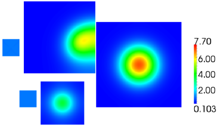
Figure 1. Snapshots of the discrete activator ($u_{1}$) profile for the Schnakenberg reaction kinetics on domains with spatially linear evolution at times 0, 590, 1000, 1750 and 2000 reading clockwise from top left. For parameter values see Table 3. We observe the formation of a half spot which reorients to a single spot positioned in the centre of the domain. As the domain contracts the spots are annihilated with the domain at end time exhibiting no patterns.

References

• Acheson [1990] D. Acheson. Elementary fluid dynamics. Oxford University Press, USA, 1990.
• Baines [1994] M. Baines. Moving finite elements. Oxford University Press, 1994.
• Baker and Maini [2007] R. Baker and P. Maini. A mechanism for morphogen-controlled domain growth. Journal of mathematical biology, 54(5):597–622, 2007.
• Barreira et al. [2011] R. Barreira, C. Elliott, and A. Madzvamuse. The surface finite element method for pattern formation on evolving biological surfaces. Journal of Mathematical Biology, pages 1–25, 2011. ISSN 0303-6812.
• Barrio et al. [2009] R. Barrio, R. Baker, B. Vaughan Jr, K. Tribuzy, M. de Carvalho, R. Bassanezi, and P. Maini. Modeling the skin pattern of fishes. Physical Review E, 79(3):31908, 2009.
• Brenner and Scott [2002] S. Brenner and L. Scott. The mathematical theory of finite element methods. Texts in Applied Mathematics, vol. 15, 2002.
• Chaplain et al. [2001] M. Chaplain, M. Ganesh, and I. Graham. Spatio-temporal pattern formation on spherical surfaces: numerical simulation and application to solid tumour growth. Journal of Mathematical Biology, 42(5):387–423, 2001. ISSN 0303-6812.
• Chueh et al. [1977] K. Chueh, C. Conley, and J. Smoller. Positively invariant regions for systems of nonlinear diffusion equations. Indiana Univ. Math. J, 26(2):373–392, 1977.
• Clément [1975] P. Clément. Approximation by finite element functions using local regularization. RAIRO, Rouge, Anal. Numér., 9(R-2):77–84, 1975.
• Crampin et al. [1999] E. Crampin, E. Gaffney, and P. Maini. Reaction and diffusion on growing domains: Scenarios for robust pattern formation. Bulletin of Mathematical Biology, 61(6):1093–1120, 1999.
• Crouzeix and Thomée [1987] M. Crouzeix and V. Thomée. The stability in $l_{p}$ and $w_{p}^{1}$ of the $l_{2}$-projection onto finite element function spaces. Mathematics of Computation, 48(178):pp. 521–532, 1987. ISSN 00255718. URL http://www.jstor.org/stable/2007825.
• Dupont [1982] T. Dupont. Mesh modification of evolution equations. Math. Comput., 39(159):85–107, 1982.
• Elliott and Stuart [1993] C. Elliott and A. Stuart. The global dynamics of discrete semilinear parabolic equations. SIAM Journal on Numerical Analysis, 30(6):1622–1663, 1993. doi: 10.1137/0730084. URL http://epubs.siam.org/doi/abs/10.1137/0730084.
• Elliott et al. [2012] C. M. Elliott, B. Stinner, and C. Venkataraman. Modelling cell motility and chemotaxis with evolving surface finite elements. Journal of The Royal Society Interface, 2012. doi: 10.1098/rsif.2012.0276. URL http://rsif.royalsocietypublishing.org/content/early/2012/05/29/rsif.2012.0276.abstract.
• Estep et al. [2000] D. Estep, M. Larson, and R. Williams. Estimating the error of numerical solutions of systems of reaction-diffusion equations. Amer Mathematical Society, 2000. ISBN 0821820729.
• Evans [2009] L. Evans. Partial Differential Equations (Graduate Studies in Mathematics, Vol. 19). Dover, 2009.
• Evans and Gariepy [1992] L. C. Evans and R. F. Gariepy. Measure Theory and Fine Properties of Functions. CRC Press, Boca Raton, FL, 1992. ISBN 0-8493-7157-0.
• Garvie and Trenchea [2007] M. Garvie and C. Trenchea. Finite element approximation of spatially extended predator–prey interactions with the Holling type II functional response. Numerische Mathematik, 107(4):641–667, 2007.
• Gierer and Meinhardt [1972] A. Gierer and H. Meinhardt. A theory of biological pattern formation. Biological Cybernetics, 12(1):30–39, 1972.
• Henderson et al. [2004] A. Henderson, J. Ahrens, and C. Law. The ParaView Guide. Kitware Clifton Park, NY, 2004.
• Hestenes and Stiefel [1952] M. Hestenes and E. Stiefel. Methods of Conjugate Gradients for Solving Linear Systems1. Journal of Research of the National Bureau of Standards, 49(6), 1952.
• Hoff [1978] D. Hoff. Stability and convergence of finite difference methods for systems of nonlinear reaction-diffusion equations. SIAM Journal on Numerical Analysis, 15(6):pp. 1161–1177, 1978. ISSN 00361429. URL http://www.jstor.org/stable/2156733.
• Kondo and Asai [1995] S. Kondo and R. Asai. A reaction–diffusion wave on the skin of the marine angelfish Pomacanthus. Nature, 376(6543):765–768, 1995.
• Labadie [2008] M. Labadie. The stabilizing effect of growth on pattern formation. Preprint, 2008.
• Lefever and Prigogine [1968] R. Lefever and I. Prigogine. Symmetry-breaking instabilities in dissipative systems II. J. chem. Phys, 48:1695–1700, 1968.
• Mackenzie and Madzvamuse [2011] J. Mackenzie and A. Madzvamuse. Analysis of stability and convergence of finite-difference methods for a reaction–diffusion problem on a one-dimensional growing domain. IMA Journal of Numerical Analysis, 31(1):212, 2011. ISSN 0272-4979.
• Madzvamuse [2000] A. Madzvamuse. A Numerical Approach to the Study of Spatial Pattern Formation. PhD thesis, University of Oxford, 2000.
• Madzvamuse [2006] A. Madzvamuse. Time-stepping schemes for moving grid finite elements applied to reaction-diffusion systems on fixed and growing domains. J. Comput. Phys., 214(1):239–263, 2006. ISSN 0021-9991.
• McKenna and Reichel [2007] P. McKenna and W. Reichel. Gidas–Ni–Nirenberg results for finite difference equations: Estimates of approximate symmetry. Journal of Mathematical Analysis and Applications, 334(1):206–222, 2007.
• Miller [1981] K. Miller. Moving finite elements. ii. SIAM Journal on Numerical Analysis, 18(6):1033–1057, 1981.
• Miller and Miller [1981] K. Miller and R. N. Miller. Moving finite elements. i. SIAM Journal on Numerical Analysis, 18(6):1019–1032, 1981.
• Miura et al. [2006] T. Miura, K. Shiota, G. Morriss-Kay, and P. Maini. Mixed-mode pattern in Doublefoot mutant mouse limb–Turing reaction-diffusion model on a growing domain during limb development. Journal of theoretical biology, 240(4):562–573, 2006.
• Moore [1994] P. Moore. A posteriori error estimation with finite element semi-and fully discrete methods for nonlinear parabolic equations in one space dimension. SIAM journal on numerical analysis, 31(1):149–169, 1994.
• Murray [2003] J. Murray. Mathematical biology. Springer Verlag, 2003.
• Schatz et al. [1980] A. Schatz, V. Thomée, and L. Wahlbin. Maximum norm stability and error estimates in parabolic finite element equations. Communications on Pure and Applied Mathematics, 33(3):265–304, 1980.
• Schmidt and Siebert [2005] A. Schmidt and K. Siebert. Design of adaptive finite element software: The finite element toolbox ALBERTA. Springer Verlag, 2005.
• Schmitt and Thompson [1998] K. Schmitt and R. Thompson. Nonlinear analysis and differential equations: An introduction. Lecture Notes, University of Utah, Department of Mathematics, 1998.
• Schnakenberg [1979] J. Schnakenberg. Simple chemical reaction systems with limit cycle behaviour. Journal of theoretical biology, 81(3):389, 1979.
• Schwab [1998] C. Schwab. p-and hp-finite element methods: Theory and applications in solid and fluid mechanics. Oxford University Press, USA, 1998. ISBN 0198503903.
• Smoller [1994] J. Smoller. Shock waves and reaction-diffusion equations. Springer, 1994.
• Thomée [2006] V. Thomée. Galerkin finite element methods for parabolic problems, volume 25 of Springer Series in Computational Mathematics. Springer-Verlag, Berlin, second edition, 2006. ISBN 978-3-540-33121-6; 3-540-33121-2.
• Thomée and Wahlbin [1975] V. Thomée and L. Wahlbin. On galerkin methods in semilinear parabolic problems. SIAM Journal on Numerical Analysis, 12(3):378–389, 1975.
• Turing [1952] A. Turing. The chemical basis of morphogenesis. Philosophical Transactions of the Royal Society of London. Series B, Biological Sciences, 237(641):37–72, 1952.
• Venkataraman et al. [2011] C. Venkataraman, T. Sekimura, E. Gaffney, P. Maini, and A. Madzvamuse. Modeling parr-mark pattern formation during the early development of amago trout. Phys. Rev. E, 84:041923, Oct 2011. doi: 10.1103/PhysRevE.84.041923. URL http://link.aps.org/doi/10.1103/PhysRevE.84.041923.
• Venkataraman et al. [2012] C. Venkataraman, O. Lakkis, and A. Madzvamuse. Global existence for semilinear reaction–diffusion systems on evolving domains. Journal of Mathematical Biology, 64:41–67, 2012. ISSN 0303-6812. URL http://dx.doi.org/10.1007/s00285-011-0404-x. 10.1007/s00285-011-0404-x.
• Venkataraman et al. [2013] C. Venkataraman, O. Lakkis, and A. Madzvamuse. Adaptive finite elements for semilinear reaction-diffusion systems on growing domains. Numerical Mathematics and Advanced Applications 2011, page 71, 2013.
• Wheeler [1973] M. Wheeler. A priori $L^{2}$ error estimates for galerkin approximations to parabolic partial differential equations. SIAM Journal on Numerical Analysis, 10(4):723–759, 1973. ISSN 0036-1429.
• Zegeling and Kok [2004] P. A. Zegeling and H. P. Kok. Adaptive moving mesh computations for reaction–diffusion systems. J. Comput. Appl. Math., 168(1-2):519–528, 2004. ISSN 0377-0427. doi: 10.1016/j.cam.2003.06.013.
• Zhang et al. [2008] K. Zhang, J. Wong, and R. Zhang. Second-order implicit-explicit scheme for the Gray-Scott model. Journal of Computational and Applied Mathematics, 213(2):559–581, 2008.