Multi-fluid cosmology: An illustration of fundamental principles

Abstract

Our current understanding of the Universe depends on the interplay of several distinct “matter” components, which interact mainly through gravity, and electromagnetic radiation. The nature of the different components, and possible interactions, tends to be based on the notion of coupled perfect fluids (or scalar fields). This approach is somewhat naive, especially if one wants to be able to consider issues involving heat flow, dissipative mechanisms, or Bose-Einstein condensation of dark matter. We argue that a more natural starting point would be the multi-purpose variational relativistic multi-fluid system that has so far mainly been applied to neutron star astrophysics. As an illustration of the fundamental principles involved, we develop the formalism for determining the non-linear cosmological solutions to the Einstein equations for a general relativistic two-fluid model for a coupled system of matter (non-zero rest mass) and “radiation” (zero rest mass). The two fluids are allowed to interpenetrate and exhibit a relative flow with respect to each other, implying, in general, an anisotropic Universe. We use initial conditions such that the massless fluid flux dominates early on so that the situation is effectively that of a single fluid and one has the usual Friedmann-Lemaître-Robertson-Walker (FLRW) spacetime. We find that there is a Bianchi I transition epoch out of which the matter flux dominates. The situation is then effectively that of a single fluid and the spacetime evolves towards the FLRW form. Such a transition opens up the possiblity of imprinting observable consequences at the specific scale corresponding to the transition time.

I Introduction

The cosmological principle states that the Universe is homogeneous and isotropic. Given the increased quality of cosmological observations, this fundamental principle is now becoming testable, and indeed questionable. That questions abound in this area is obvious from the fact that we do not have a good handle on the nature of dark components that dominate the cosmological “standard model” Peter and Uzan (2009). A large number of alternative models and theories have been suggested in the literature, but most are not particularly compelling. The treatment of the different matter components, in particular, is often based on the notion of coupled perfect fluids or scalar fields. If we are to understand the bigger picture, we need to make progress on this aspect, especially if we want to be able to consider issues like heat flow Modak (1984); Triginer and Pavon (1995); Andersson and Lopez-Monsalvo (2011), dissipative mechanisms Weinberg (1971); Patel and Koppar (1991); Velten and Schwarz (2011), Bose-Einstein condensation of dark matter Sikivie and Yang (2009); Harko (2011) and possibly many others.

We argue that a more natural starting point for this endeavor would be the relativistic variational multi-fluid approach Carter (1989) that has (so far) mainly been applied to neutron star astrophysics Andersson and Comer (2007), and recently to relativistic beams and shocks Nakar et al. (2011). This approach would seem natural since there could have been phases during which the Universe would have effectively been anisotropic, with different components evolving “independently”. For the most part, models discussed in the current literature, including initially anisotropic geometries, describe the matter content in terms of either effectively many component single fluid models Gromov et al. (2004), or a plain single component Emir Gümrükçüoglu et al. (2007); Pitrou et al. (2008); Kim and Minamitsuji (2010); although isotropisation is expected in such situations, as required to end up with a realistic (read: in agreement with currently available data) model Dechant et al. (2009), interesting new consequences can however be derived, e.g. by enhancing an initially vanishingly small non-gaussian signal Dey and Paban (2011).

As an illustration of the fundamental principles involved, we develop the formalism for determining the cosmological solutions to the Einstein equations for a general relativistic, two-fluid model coupling matter (non-zero rest mass) and “radiation” (zero rest mass). Drawing on the experience from other applications it would be straightforward to consider other relevant cases, e.g. involving a dissipative heat flow Andersson and Lopez-Monsalvo (2011) or superfluid condensates Sikivie and Yang (2009); Harko (2011). However, the chosen example is perhaps the most conventional, since the leading-order thermodynamics of massless particles has some generic features (compare, say, a photon and phonon gas), and the same for a massive component when the density becomes (relatively) small.

Within this context, we will demonstrate how the distinct fluid motions lead to anisotropy and the spacetime metric taking the form of a Bianchi I solution of the Einstein equations. This follows since there is a spacelike privileged vector, associated with the relative flow between the two components in the problem. It is important to understand that, while this feature is natural in the multi-fluid context, it can never arise in the often considered multi-constituent single fluid. The multi-fluid hypothesis implies that each component (labelled by an index x) of the matter and radiation sourcing Einstein equations follows its own timelike vector $u_{\mathrm{x}}^{\mu}$; the relative flow between the various fluids then generates a privileged spacelike direction along which the Bianchi I solution aligns. However, it is important to recognize that it is the fluxes $n^{\mu}_{\mathrm{x}}=n_{\mathrm{x}}u^{\mu}_{\mathrm{x}}$, where $n_{\mathrm{x}}$ is the particle number density, that are the fundamental sources. In particular, a fluid can be moving quickly with respect to another, yet if its density is much smaller its flux can be negligible.

Such a choice is by no means new Sandin (2009) and recent work in given circumstances have shown, here again, the possibility of isotropisation Harko and Lobo (2011), although behavior very different from the standard cosmological one can also be found Calogero and Heinzle (2011). (A useful review on anisotropic solutions and their cosmological use is Ref. Tsagas et al. (2008).) For instance, it has been suggested Barrow and Tsagas (2007); Adhav et al. (2011); Cataldo et al. (2011) that since Bianchi universes, seen as averaged inhomogeneous and anisotropic spacetimes, can have effective strong energy condition violating stress-energy tensors, they could be part of a backreaction driven acceleration model.

Yet another reason for studying such cosmological models stem, curiously, from the observations! Large angle anomalies in the Cosmic Microwave Background (CMB) indeed have been observed and discussed for quite some time Schwarz et al. (2004); Copi et al. (2010); Perivolaropoulos (2011); Ma et al. (2011) and related with underlying Bianchi models Pontzen and Challinor (2007); Pontzen (2009). It is not our aim here to decide whether or not the data do indeed imply some amount of anisotropy, but we shall at least assume that they do not rule out the possibility altogether. Note in that respect that further, currently ongoing observations of different backgrounds will determine, for instance, if the CMB dipole is fully originating from mere local Earth motion (and should thus be removed altogether from the data) or if part of it is cosmological Fixsen and Kashlinsky (2011).

In order to remain close to the observationally verifiable model, we shall concentrate on the example of the radiation to matter transition for which, in principle, the underlying microphysics ought to be well-known, up to the a priori necessarily negligible Dark-Matter to radiation coupling. We then ask whether it is possible to have a cosmological epoch where there is a relative flow of radiation with respect to the matter, but out of which the expansion becomes isotropic and the relative flow dissipates. We will demonstrate that the short answer to this question is yes, as flux domination of one fluid over the other leads to an effectively one-fluid situation, thus yielding an effective Friedman-Lemaître-Robertson-Walker (FLRW) Universe. In essence, the cosmological principle appears to be satisfied on both sides of the transition, but the transition itself puts forward a Bianchi I behavior with a spacelike privileged direction. Our goal here is to, first of all, establish this possibility and then consider the compatibility of such a model with current observational data Komatsu et al. (2011); Percival et al. (2010).

On the technical side, the two-fluid nature of the problem introduces several terms that are not present in the one-fluid case. We will “skew” the discussion somewhat by introducing variables that were found useful in the stability analysis of two-fluid systems by Samuelsson et al. Samuelsson et al. (2010). In particular, we will take into account the fact that two-fluid systems have two speeds of “sound”, and use causality to constrain parameter values that enter through the equation of state. We will also introduce the so-called cross- constituent coupling, which occurs when the equation of state has terms containing both fluid densities. It is an equilibrium property and thus is non- dissipative. While the coupling is not the main focus here, it is important for a follow-on analysis Comer et al. (2011) where we consider so-called two-stream instability. This can occur when there is a relative flow between two fluids with cross-constituent coupling. If a disturbance is developed on top of the relative flow, and the coupling is strong enough, it can become unstable if it appears to move, say, to the right with respect to one fluid, but to the left with respect to the other. In this sense, the work here has the additional purpose of building the “background”, relative-flow configurations.

The outline of this paper is as follows: In Sec. II we construct cosmologies having two Killing symmetries, with the subsequent Einstein tensor components presented in Sec. II.1. Sec. II.2 contains a brief review of the two-fluid formalism and how it applies in the current context. We also show how our formalism can be immediately employed to describe relativistic condensates (which reduces to the standard descriptions of terrestrial systems, such as superfluid helium four). In the following Sec. III we show how an ideal gas in the presence of a radiation field leads to a system with cross-constituent coupling, and then construct a simpler model containing similar characteristics. Sec. IV restricts the analysis by removing the spatial-dependence in the metric and matter. (The more general set of equations are required for the two-stream instability analysis of Comer et al. (2011).) This same section includes a numerical analysis subsection IV.2 and ends with a discussion of the results. We finish with some concluding remarks in Sec. V and an appendix containing more details on how the equations are obtained.

II Cosmologies with Two Spacelike Killing Vectors

We will choose the simplest possible two-fluid model: the relative matter flow is in one direction (to be taken along the $z$ “axis”), and orthogonal to it will be two, mutually orthogonal spacelike Killing vector fields (one along the $x$ “axis” and another along the $y$ “axis”). We will use as our $x$ and $y$ coordinates the two parameters that naturally generate the Killing vector fields ${\cal X}^{\mu}$ and ${\cal Y}^{\mu}$. With this choice we have

$${\cal X}^{\mu}=(0,1,0,0)\quad,\quad{\cal Y}^{\mu}=(0,0,1,0).$$ (1)

It is also the case that

$$0=g_{\mu\nu}{\cal X}^{\mu}{\cal Y}^{\nu}=g_{12}.$$ (2)

Finally, if we let $t$ denote the time coordinate then the two symmetries imply the remaining metric components are functions of only $z$ and $t$.

There is some remaining freedom in the choice of coordinate system, i.e. it can be shown that the so-called synchronous gauge ($g_{00}=-1$ and $g_{0i}=0$) that reduces the metric to

$$\mathrm{d}s^{2}=-\mathrm{d}t^{2}+g_{xx}\mathrm{d}x^{2}+g_{yy}\mathrm{d}y^{2}+g_{zz}\mathrm{d}z^{2}+2g_{xz}\mathrm{d}x\mathrm{d}z+2g_{yz}\mathrm{d}y\mathrm{d}z,$$ (3)

can be utilized. Within this gauge choice there is another change of coordinates that can be made, namely $\bar{t}=t$, $\bar{x}=\bar{x}(x,z)$, $\bar{y}=\bar{y}(y,z)$, and $\bar{z}=z$, that sets the terms $g_{13}$ and $g_{23}$ to zero. The final form of the metric is thus

$$\mathrm{d}s^{2}=-\mathrm{d}t^{2}+A_{x}^{2}\mathrm{d}x^{2}+A_{y}^{2}\mathrm{d}y^{2}+A_{z}^{2}\mathrm{d}z^{2},$$ (4)

where the $A_{\aleph}$ ($\aleph=\{x,y,z\}$) are, as yet unknown, functions of $t$ and $z$. When the $z$-dependence is relaxed, the spacetime described by (4) is of the well-known Bianchi I type. Although we focus on this case later in Sec. IV, we keep the $z$-dependence here because a follow-on analysis Comer et al. (2011) will need the full $z$-dependent equations.

II.1 The Einstein Tensor

The non-trivial Einstein Tensor coefficients can be straightforwardly computed with the known geometric quantities given in the Appendix. Letting a dot “$~{}\dot{}~{}$” and a prime “$~{}^{\prime}{}~{}$” denote, respectively, $\partial/\partial t$ and $\partial/\partial z$, we have

$$G^{t}{}_{t} = -\left(H_{x}H_{y}+H_{x}H_{z}+H_{y}H_{z}\right)+\frac{1}{A^{2}_{z}}\left[I^{\prime}_{x}+I^{\prime}_{y}+\left(I_{x}+I_{y}\right)^{2}-I_{x}I_{y}-I_{x}I_{z}-I_{y}I_{z}\right],$$ (5)

$$G^{x}{}_{x} = -\left(\dot{H}_{y}+\dot{H}_{z}\right)-\left(H^{2}_{y}+H_{y}H_{z}+H^{2}_{z}\right)+\frac{1}{A^{2}_{z}}\left[I^{\prime}_{y}+\left(I_{y}-I_{z}\right)I_{y}\right],$$ (7)

$$G^{y}{}_{y} = -\left(\dot{H}_{x}+\dot{H}_{z}\right)-\left(H^{2}_{x}+H_{x}H_{z}+H^{2}_{z}\right)+\frac{1}{A^{2}_{z}}\left[I^{\prime}_{x}+\left(I_{x}-I_{z}\right)I_{x}\right],$$ (9)

$$G^{z}{}_{t} = -\frac{1}{A^{2}_{z}}\left[\dot{I}_{x}+\dot{I}_{y}+\left(H_{x}-H_{z}\right)I_{x}+\left(H_{y}-H_{z}\right)I_{y}\right],$$ (11)

$$G^{z}{}_{z} = -\left(\dot{H}_{x}+\dot{H}_{y}\right)-\left(H^{2}_{x}+H_{x}H_{y}+H^{2}_{y}\right)+\frac{I_{x}I_{y}}{A^{2}_{z}},$$ (13)

where we have introduced the “Hubble”-like functions ($\aleph=\{x,y,z\}$)

$$H_{\aleph}\equiv\frac{\dot{A}_{\aleph}}{A_{\aleph}},$$ (14)

and the “inhomogeneity” functions

$$I_{\aleph}\equiv\frac{A^{\prime}_{\aleph}}{A_{\aleph}}.$$ (15)

We will see below that when the $z$-dependence is dropped, the two-fluid energy-momentum-stress components are such that $T^{x}{}_{x}=T^{y}{}_{y}$, implying for the Einstein tensor $G^{x}{}_{x}=G^{y}{}_{y}$.

Clearly, not all these components can be independent of each other, for otherwise the overall problem would be ill-posed because of too many equations. But recall that there is the Bianchi Identity $\nabla_{\nu}G^{\nu}{}_{\mu}=0$, which for the situation here yields two independent components:

$$0 = \dot{G}^{t}{}_{t}+\partial_{z}G^{z}{}_{t}+\left(H_{x}+H_{y}+H_{z}\right)G^{t}{}_{t}+\left(I_{x}+I_{y}+I_{z}\right)G^{z}{}_{t}-H_{x}G^{x}{}_{x}-H_{y}G^{y}{}_{y}-H_{z}G^{z}{}_{z},$$ (16)

$$0 = \dot{G}^{t}{}_{z}+\partial_{z}G^{z}{}_{z}+\left(H_{x}+H_{y}+H_{z}\right)G^{t}{}_{z}+\left(I_{x}+I_{y}\right)\left(G^{z}{}_{z}-G^{x}{}_{x}\right).$$ (18)

It is important to note that the second of these vanishes identically when there is no $z$-dependence, because then the Einstein tensor component $G^{z}_{t}=0$. This means that we still need three metric degrees of freedom.

II.2 General Relativistic Two-fluid Formalism

We will use the formalism developed by Carter Carter (1989) and various collaborators (see Andersson and Comer Andersson and Comer (2007) for a review and references). The fundamental fluid variables consist of two conserved number density four-currents, to be denoted $n^{\mu}_{\mathrm{x}}$. Recall that $\mathrm{x}$ is a constituent index (for which there is no implied sum when repeated).

From the currents, we can form three scalars, namely $n_{\mathrm{x}}^{2}=-g_{\mu\nu}n_{\mathrm{x}}^{\mu}n_{\mathrm{x}}^{\nu}$, $n_{\mathrm{y}}^{2}=-g_{\mu\nu}n_{\mathrm{y}}^{\mu}n_{\mathrm{y}}^{\nu}$, and $n_{\mathrm{x}\mathrm{y}}^{2}=-g_{\mu\nu}n_{\mathrm{x}}^{\mu}n_{\mathrm{y}}^{\nu}$. A so-called “master” function $-\Lambda(n_{\mathrm{x}}^{2},n_{\mathrm{y}}^{2},n_{\mathrm{x}\mathrm{y}}^{2})$ (the two-fluid analog of the equation of state) is assumed, which plays the role of Lagrangian for the system. The energy-momentum-stress tensor is

$$T^{\mu}{}_{\nu}=\Psi\delta^{\mu}{}_{\nu}+n_{\mathrm{x}}^{\mu}\mu^{\mathrm{x}}_{\nu}+n_{\mathrm{y}}^{\mu}\mu^{\mathrm{y}}_{\nu},$$ (19)

where

$$\Psi=\Lambda-n_{\mathrm{x}}^{\rho}\mu^{\mathrm{x}}_{\rho}-n_{\mathrm{y}}^{\rho}\mu^{\mathrm{y}}_{\rho}$$ (20)

is the generalized pressure and

$$\mu^{\mathrm{x}}_{\nu}=g_{\nu\mu}\left({\cal B}^{\mathrm{x}}n_{\mathrm{x}}^{\mu}+{\cal A}^{\mathrm{x}\mathrm{y}}n_{\mathrm{y}}^{\mu}\right)$$ (21)

is the chemical potential covector. It is also the momentum canonically conjugate to the current $n_{\mathrm{x}}^{\mu}$.

Formally, the ${\cal A}^{\mathrm{x}\mathrm{y}}$ and ${\cal B}^{\mathrm{x}}$ coefficients are obtained from $\Lambda$ via the partial derivatives

$${\cal A}^{\mathrm{x}\mathrm{y}}={\cal A}^{\mathrm{y}\mathrm{x}}=-\frac{\partial\Lambda}{\partial n_{\mathrm{x}\mathrm{y}}^{2}}\quad,\quad{\cal B}^{\mathrm{x}}=-2\frac{\partial\Lambda}{\partial n_{\mathrm{x}}^{2}}.$$ (22)

The fact that the momentum $\mu^{\mathrm{x}}_{\mu}$ is not simply proportional to the corresponding number density current $n_{\mathrm{x}}^{\mu}$ is a result of entrainment (as it is known in the neutron star literature; see, for example, Comer and Joynt (2003)): the motion of one fluid induces a momentum in the other fluid, and vice versa. Entrainment vanishes if the ${\cal A}^{\mathrm{x}\mathrm{y}}$ coefficient is zero.

Finally, the equations for each fluid consists of a conservation equation

$$\nabla_{\mu}n_{\mathrm{x}}^{\mu}=0,$$ (23)

and an Euler equation

$$n_{\mathrm{x}}^{\mu}\omega^{\mathrm{x}}_{\mu\nu}=0,$$ (24)

where the vorticity two-form is defined by

$$\omega^{\mathrm{x}}_{\mu\nu}=2\nabla_{[\mu}\mu^{\mathrm{x}}_{\nu]},$$ (25)

the square brackets indicating antisymmetrization of the enclosed indices. It is important to understand that the condition $\nabla_{\mu}T^{\mu}{}_{\nu}=0$ is satisfied once the equations of motion are satisfied. Contrary to the single-fluid case, $\nabla_{\mu}T^{\mu}{}_{\nu}=0$ does not yield enough information to completely determine the two-fluid evolution.

Note that the above way of writing each Euler equation makes manifest its geometric meaning as an integrability condition for the corresponding vorticity, a point that has been much emphasized by Carter Carter (1989) (see also Andersson and Comer (2007)). It also immediately supplies a formalism for superfluid condensates, since setting $\mu^{\mathrm{x}}_{\nu}=\nabla_{\nu}\Phi_{\mathrm{x}}$ (where $\Phi_{\mathrm{x}}$ represents the phase of the relevant quantum wavefunction) guarantees that the fluid vorticity is zero. The non-relativistic limit of the fluid equations in this case recovers those that are well-known for, say, helium superfluids.

The symmetries do much to simplify the fluid equations. It is easy to see that the vanishing of the Lie derivative of $n_{\mathrm{x}}^{\mu}$ with respect to ${\cal X}^{\mu}$ and ${\cal Y}^{\mu}$ requires $n_{\mathrm{x}}^{\mu}$ to be a function only of $t$ and $z$. We also assume that $n_{\mathrm{x}}^{\mu}$ is orthogonal to ${\cal X}^{\mu}$ and ${\cal Y}^{\mu}$. The unit four-vectors take the form

$$u^{\nu}_{\mathrm{x}}=\left(u^{t}_{\mathrm{x}},0,0,u^{z}_{\mathrm{x}}\right)\quad,\quad u^{t}_{\mathrm{x}}=\sqrt{1+\left(A_{z}u^{z}_{\mathrm{x}}\right)^{2}}.$$ (26)

The entrainment parameter becomes

$$n_{\mathrm{x}\mathrm{y}}^{2}=n_{\mathrm{x}}n_{\mathrm{y}}\left(u^{t}_{\mathrm{x}}u^{t}_{\mathrm{y}}-A^{2}_{z}u^{z}_{\mathrm{x}}u^{z}_{\mathrm{y}}\right),$$ (27)

while the momenta reduce to

$$\mu^{\mathrm{x}}_{t} = -\left({\cal B}^{\mathrm{x}}n_{\mathrm{x}}u^{t}_{\mathrm{x}}+{\cal A}^{\mathrm{x}\mathrm{y}}n_{\mathrm{y}}u^{t}_{\mathrm{y}}\right),$$ (28)

$$\mu^{\mathrm{x}}_{z} = A_{z}^{2}\left({\cal B}^{\mathrm{x}}n_{\mathrm{x}}u^{z}_{\mathrm{x}}+{\cal A}^{\mathrm{x}\mathrm{y}}n_{\mathrm{y}}u^{z}_{\mathrm{y}}\right).$$ (30)

Finally, the components of $T^{\mu}{}_{\nu}$ are

$$T^{t}{}_{t} = \Psi+n_{\mathrm{x}}u^{t}_{\mathrm{x}}\mu^{\mathrm{x}}_{t}+n_{\mathrm{y}}u^{t}_{\mathrm{y}}\mu^{\mathrm{y}}_{t},$$ (31)

$$T^{x}{}_{x} = T^{y}{}_{y}=\Psi,$$ (33)

$$T^{z}{}_{t} = n_{\mathrm{x}}u^{z}_{\mathrm{x}}\mu^{\mathrm{x}}_{t}+n_{\mathrm{y}}u^{z}_{\mathrm{y}}\mu^{\mathrm{y}}_{t},$$ (35)

$$T^{z}{}_{z} = \Psi+n_{\mathrm{x}}u^{z}_{\mathrm{x}}\mu^{\mathrm{x}}_{z}+n_{\mathrm{y}}u^{z}_{\mathrm{y}}\mu^{\mathrm{y}}_{z},$$ (37)

where

$$\Psi=\Lambda-n_{\mathrm{x}}\left(u^{t}_{\mathrm{x}}\mu^{\mathrm{x}}_{t}+u^{z}_{\mathrm{x}}\mu^{\mathrm{x}}_{z}\right)-n_{\mathrm{y}}\left(u^{t}_{\mathrm{y}}\mu^{\mathrm{y}}_{t}+u^{z}_{\mathrm{y}}\mu^{\mathrm{y}}_{z}\right).$$ (38)

The remaining item required to completely specify the matter is a particular form for the master function $\Lambda$. This we will provide in Section III.

We see from the above that our problem has been reduced to finding solutions for the four matter variables $\{n_{\mathrm{x}},u^{z}_{\mathrm{x}}\}$ and the three metric functions $A_{\aleph}$. The conservation equations (23) now take the form

$$0=\frac{\partial}{\partial t}\left(A_{x}A_{y}A_{z}n_{\mathrm{x}}u^{t}_{\mathrm{x}}\right)+\frac{\partial}{\partial z}\left(A_{x}A_{y}A_{z}n_{\mathrm{x}}u^{z}_{\mathrm{x}}\right),$$ (39)

while the Euler equations reduce to

$$\frac{\partial\mu^{\mathrm{x}}_{t}}{\partial z}=\frac{\partial\mu^{\mathrm{x}}_{z}}{\partial t}.$$ (40)

The remaining equations are those of Einstein, constructed from Eqs. (13) and (37).

As mentioned in the introduction, we introduce some new variables that are convenient for the multi-fluid analysis. Since there are two fluids we have the well-established result of two modes of “sound” propagation Carter (1989); namely,

$$c_{\mathrm{x}}^{2}\equiv\frac{\partial\ln\mu^{\mathrm{x}}}{\partial\ln n_{\mathrm{x}}}.$$ (41)

These are “bare” in the sense that they only equal the local wave speed when there are no interactions between the fluids Samuelsson et al. (2010). A measure of the interactions are the cross-constituent couplings defined—slightly modified from Samuelsson et al. (2010)—as

$$\mathcal{C}_{\mathrm{x}\mathrm{y}}\equiv\frac{\partial\ln\mu^{\mathrm{x}}}{\partial\ln n_{\mathrm{y}}}=\frac{\mu^{\mathrm{y}}n_{\mathrm{y}}}{\mu^{\mathrm{x}}n_{\mathrm{x}}}\mathcal{C}_{\mathrm{y}\mathrm{x}},$$ (42)

where, if we set the entrainment to zero,

$$\mu^{\mathrm{x}}\equiv-u^{\nu}_{\mathrm{x}}\mu^{x}_{\nu}={\cal B}^{\mathrm{x}}n_{\mathrm{x}}.$$ (43)

The $\mathcal{C}_{\mathrm{x}\mathrm{y}}$ represent a key channel through which the two fluids “see” each other (especially when the entrainment is zero) Samuelsson et al. (2010); Comer et al. (2011).

Some final words on this set-up is about our frame of reference. We have chosen a frame that is not attached to either fluid. One might expect it would be easier to work in either of the fluid rest-frames, but this is actually not the case. Starting with the metric in Eq. (4), we can show that “jumping” on a fluid rest-frame introduces a shift vector into the metric.

Let $\bar{x}^{\mu}$ be the rest-frame coordinates of, say, the $\mathrm{x}$-fluid. We can assume that the coordinate transformation does not involve the orthogonal pair $\{x,y\}$, so that $\bar{t}=\bar{t}(t,z)$, $\bar{x}=x$, $\bar{y}=y$, and $\bar{z}=\bar{z}(t,z)$, which guarantees $\bar{u}^{x}_{\mathrm{x}}=\bar{u}^{y}_{\mathrm{x}}=0$. What we want is $\bar{u}^{z}_{\mathrm{x}}=0$, which implies

$$\frac{\partial\bar{z}}{\partial t}=-\frac{\partial\bar{z}}{\partial z}\frac{u^{z}_{\mathrm{x}}}{u^{t}_{\mathrm{x}}},$$ (44)

and therefore $\bar{z}$ must depend on both $t$ and $z$. We can now assume that $\bar{t}=t$. However, the change of coordinates also affects the metric; in particular,

$$\bar{g}^{tz}=-\frac{\partial\bar{z}}{\partial t}\neq 0.$$ (45)

III A Cosmological Two-fluid Scenario: Matter and Radiation

When the particle species of a fluid has mass $m^{\mathrm{x}}$, it can be useful to separate out from $\Lambda$ mass density terms; namely,

$$\Lambda=-m^{\mathrm{x}}n_{\mathrm{x}}-m^{\mathrm{y}}n_{\mathrm{y}}-{\cal E}(n_{\mathrm{x}}^{2},n_{\mathrm{y}}^{2},n_{\mathrm{x}\mathrm{y}}^{2})\ ,$$ (46)

where ${\cal E}$ contains other information about the fluid thermodynamics, and relative motion effects. The two-fluid cosmology we have in mind has a combination of “matter”, with mass $m^{\mathrm{x}}=m$, and “radiation”, which means $m^{\mathrm{y}}=0$. We assume a non-zero cross-constituent coupling and zero entrainment. One of our conserved currents is the total particle flux of the matter. Since we are ignoring dissipation in the flows, we can use the total entropy flux of the system as our other conserved current. The bulk of this is due to the radiation. To simplify the notation, we set $n_{\mathrm{x}}=n$, $n_{\mathrm{y}}=s$, $\mu^{\mathrm{x}}\equiv\mu$, and $\mu^{\mathrm{y}}\equiv T$, which is the temperature.

To see how a cross-constituent term can come about, consider the usual way of combining a (non-relativistic) gas and radiation in the energy density and pressure:

$$\rho = mn+\frac{3}{2}nT+\alpha T^{4},$$ (47)

$$p = nT+\frac{1}{3}\alpha T^{4},$$ (49)

where $\alpha$ is constant. We take as our fundamental thermodynamic variables $n$ and $s$, and so the temperature, obtained as $T=\partial\rho/\partial s$, is a function of both. Hence, the ideal gas contribution will generate a cross-constituent coupling (cf. Eq. (42)). Even if we take the temperature as fundamental, there would still be its coupling with $n$.

Writing $T$ in terms of $\{n,s\}$ explicitly is not tractable. So for the purpose at hand, it is perhaps clearer to consider a simpler, algebraic construction where the dependence is explicit. With that in mind, we will use a master function of the form

$$\Lambda=-m^{*}n-\kappa_{\mathrm{s}}s^{4/3},$$ (50)

where we have placed a polytropic coupling to the entropy in an effective mass $m^{*}$ for the matter; namely,

$$m^{*}=m+\tau_{\mathrm{n}\mathrm{s}}n^{\sigma_{\mathrm{n}}-1}s^{\sigma_{\mathrm{s}}},$$ (51)

where $\sigma_{\mathrm{n}}\geq 1$, $\sigma_{\mathrm{s}}\geq 1$, and $\tau_{\mathrm{n}\mathrm{s}}$ are constants. The remaining fluid variables are

$$\Psi = \frac{1}{3}\kappa_{\mathrm{s}}s^{4/3}+\left(\sigma_{\mathrm{n}}+\sigma_{\mathrm{s}}-1\right)\left(m^{*}-m\right)n,$$ (52)

$$\mu = m+\sigma_{\mathrm{n}}\left(m^{*}-m\right),$$ (54)

$$T = \frac{4}{3}\kappa_{\mathrm{s}}s^{1/3}+\sigma_{\mathrm{s}}\left(m^{*}-m\right)\frac{n}{s},$$ (56)

$$\mathcal{C}_{\mathrm{n}\mathrm{s}} = \frac{\sigma_{\mathrm{s}}}{\sigma_{\mathrm{n}}-1}c_{\mathrm{n}}^{2},$$ (58)

where

$$\mu c_{\mathrm{n}}^{2} = \sigma_{\mathrm{n}}\left(\sigma_{\mathrm{n}}-1\right)\left(m^{*}-m\right),$$ (59)

$$Tc_{\mathrm{s}}^{2} = \frac{4}{9}\kappa_{\mathrm{s}}s^{1/3}+\sigma_{\mathrm{s}}\left(\sigma_{\mathrm{s}}-1\right)\left(m^{*}-m\right)\frac{n}{s}.$$ (61)

There are a few comments to be made about this construction. In order to have a model that cools as it expands, we see that $n\to 0$ and $s\to 0$ which also means $m^{*}\to m$. This also ensures that the “dust” limit of the standard cosmological scenario $\mu\to m$ and $c_{\mathrm{n}}\to 0$ is achieved. Finally, we recover the usual result for the massless fluid of $s\propto T^{3}$ and $c_{\mathrm{s}}^{2}\to 1/3$. In fact, if we eliminate the second term in (61) using (56), we find

$$s=\sigma T^{3}\quad\hbox{and}\quad\sigma=\left[\frac{3\left(\sigma_{\mathrm{s}}-1-c_{\mathrm{s}}^{2}\right)}{4\left(\sigma_{\mathrm{s}}-4/3\right)\kappa_{\mathrm{s}}}\right]^{3}.$$ (62)

It is also worthwhile to consider the other direction of the evolution, which is that back to the past, where the universe contracts and heats up to the point where the temperature scale is much higher than that of the mass scale.

IV Homogeneous Background

Assuming that the background is only time-dependent, then the two matter equations (39) and (40) imply (for $\mathrm{x}=\{\mathrm{n},\mathrm{s}\}$)

$$A_{z}\mu^{\mathrm{x}}V_{\mathrm{x}}={\cal M}_{\mathrm{x}}\quad,\quad A_{x}A_{y}A_{z}n_{\mathrm{x}}\sqrt{1+V_{\mathrm{x}}^{2}}={\cal N}_{\mathrm{x}},$$ (63)

where ${\cal M}_{\mathrm{x}}$ and ${\cal N}_{\mathrm{x}}$ are constants and we have introduced $V_{\mathrm{x}}=A_{z}u^{z}_{\mathrm{x}}$. One can also show that $T^{z}{}_{t}=0$ is automatically guaranteed by (63), provided that the integration constants satisfy

$${\cal M}_{\mathrm{n}}{\cal N}_{\mathrm{n}}+{\cal M}_{\mathrm{s}}{\cal N}_{\mathrm{s}}=0.$$ (64)

Equation (63) allows, in principle, to write $n_{\mathrm{x}}$ and $V_{\mathrm{x}}$ in terms of $A_{\aleph}$, which can be put into the Einstein equations to get a closed system of equations. But, since we will be solving the equations numerically, it is actually easier to use the original differential equations, which can be shown to take the form

$$\left(\begin{array}[]{cc}1-\displaystyle\frac{c_{\mathrm{n}}^{2}V_{\mathrm{n}}^{2}}{1+V_{\mathrm{n}}^{2}}&-\displaystyle\frac{\mathcal{C}_{\mathrm{n}\mathrm{s}}V_{\mathrm{n}}^{2}}{1+V_{\mathrm{n}}^{2}}\\ \\ -\displaystyle\frac{\mathcal{C}_{\mathrm{s}\mathrm{n}}V_{\mathrm{s}}^{2}}{1+V_{\mathrm{s}}^{2}}&1-\displaystyle\frac{c_{\mathrm{s}}^{2}V_{\mathrm{s}}^{2}}{1+V_{\mathrm{s}}^{2}}\end{array}\right)\left(\begin{array}[]{c}\displaystyle\frac{\dot{n}}{n}\\ \\ \displaystyle\frac{\dot{s}}{s}\end{array}\right)=-\left(\begin{array}[]{c}H_{x}+H_{y}+\displaystyle\frac{H_{z}}{1+V_{\mathrm{n}}^{2}}\\ \\ H_{x}+H_{y}+\displaystyle\frac{H_{z}}{1+V_{\mathrm{s}}^{2}}\end{array}\right)$$ (65)

for the densities and

$$\left(\begin{array}[]{c}\displaystyle\frac{\dot{V}_{\mathrm{n}}}{V_{\mathrm{n}}}\\ \\ \displaystyle\frac{\dot{V}_{\mathrm{s}}}{V_{\mathrm{s}}}\end{array}\right)=-\left(\begin{array}[]{cc}c_{\mathrm{n}}^{2}&\mathcal{C}_{\mathrm{n}\mathrm{s}}\\ \\ \mathcal{C}_{\mathrm{s}\mathrm{n}}&c_{\mathrm{s}}^{2}\end{array}\right)\left(\begin{array}[]{c}\displaystyle\frac{\dot{n}}{n}\\ \\ \displaystyle\frac{\dot{s}}{s}\end{array}\right)-\left(\begin{array}[]{c}H_{z}\\ \\ H_{z}\end{array}\right)$$ (66)

for the velocities.

To solve for the metric we use the definition of $H_{\aleph}$ and three of the Einstein equations (setting $G_{{}_{\mathrm{N}}}=M_{{}_{\mathrm{Pl}}}^{-2}$ with $M_{{}_{\mathrm{Pl}}}$ the Planck mass) to evolve $\{A_{\aleph},H_{\aleph}\}$ as follows:

$$\dot{H}_{x} = -H^{2}_{x}+H_{y}H_{z}-\frac{4\pi}{M_{{}_{\mathrm{Pl}}}^{2}}\left[\mu n\left(1+2V_{\mathrm{n}}^{2}\right)+Ts\left(1+2V_{\mathrm{s}}^{2}\right)\right],$$ (67)

$$\dot{H}_{y} = -H^{2}_{y}+H_{x}H_{z}-\frac{4\pi}{M_{{}_{\mathrm{Pl}}}^{2}}\left[\mu n\left(1+2V_{\mathrm{n}}^{2}\right)+Ts\left(1+2V_{\mathrm{s}}^{2}\right)\right],$$ (69)

$$\dot{H}_{z} = -H^{2}_{z}+H_{x}H_{y}-\frac{4\pi}{M_{{}_{\mathrm{Pl}}}^{2}}\left(\mu n+Ts\right),$$ (71)

$$\dot{A}_{\aleph} = H_{\aleph}A_{\aleph}.$$

The so-called Hamiltonian constraint $G^{t}{}_{t}=\displaystyle\frac{8\pi}{M_{{}_{\mathrm{Pl}}}^{2}}T^{t}{}_{t}$ is

$$H_{x}H_{y}+H_{x}H_{z}+H_{y}H_{z}=\frac{8\pi}{M_{{}_{\mathrm{Pl}}}^{2}}\left(-\Lambda+\mu nV_{\mathrm{n}}^{2}+TsV_{\mathrm{s}}^{2}\right).$$ (73)

The initial conditions therefore consist of four matter, and six metric initial conditions; i.e. the set $\{n(t_{0}),s(t_{0}),V_{\mathrm{n}}(t_{0}),V_{\mathrm{s}}(t_{0}),A_{\aleph}(t_{0}),H_{\aleph}(t_{0})\}$, where $t_{0}$ is the initial time.

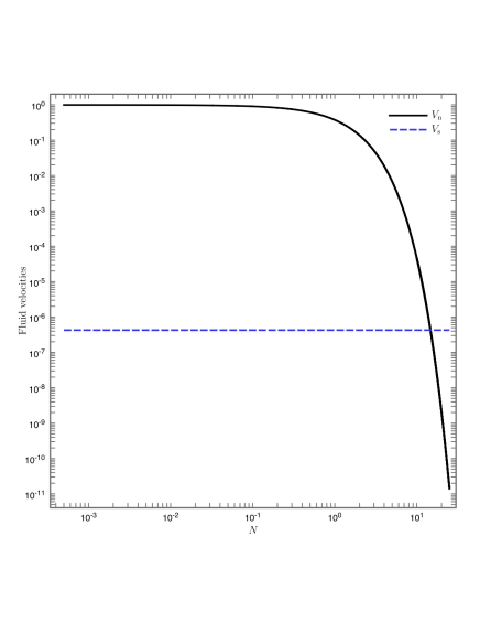
Figure 1: Velocities derived from Eq. (66), as functions of the e-fold number $N$ (defined in the main text). The underlying parameter values for this plot are $\kappa_{\mathrm{s}}=1$, $\tilde{\tau}=0.1$, $\sigma_{\mathrm{n}}=1.1$, and $\sigma_{\mathrm{s}}=1.1$. The initial values are such that $n(0)=3.9\times 10^{-7}$, $s(0)=1$, $V_{\mathrm{n}}(0)=0.99$, $V_{\mathrm{s}}(0)=-4.25\times 10^{-7}$, $A_{\aleph}(0)=2$, and $H_{\aleph}(0)=2.89$ (for each $\aleph$). This figure illustrates that $V_{\mathrm{n}}$, although initially very large, rapidly decays to zero while $V_{\mathrm{s}}$ remains essentially negligible, and almost constant, at all times.

IV.1 Preliminaries: The Matter Quadratures

It is useful at this point to apply the results of Eq. (63). For the matter we can write

$$n = \frac{1}{A_{x}A_{y}A_{z}}\frac{{\cal N}_{\mathrm{n}}}{\sqrt{1+{\cal M}_{\mathrm{n}}^{2}/\left(A_{z}\mu\right)^{2}}},$$ (74)

$$V_{\mathrm{n}} = \frac{{\cal M}_{\mathrm{n}}}{A_{z}\mu}.$$ (76)

The first indicates that the metric coefficients must grow with time if both $n\to 0$ and $\mu\to m$ (the conditions for cooling); that is, we can be sure that our model allows for both expansion and cooling. The second relation therefore shows that $V_{\mathrm{n}}\to 0$ with time.

A similar analysis for the entropy fluid is complicated by the fact that it is massless, and thus the associated chemical potential (i.e. the temperature) can go to zero. In particular, it is not clear a priori that the entropy fluid velocity

$$V_{\mathrm{s}}=\frac{{\cal M}_{\mathrm{s}}}{A_{z}T}$$ (77)

remains finite, i.e. whether or not $A_{z}T$ grows with time. Actually, the entropy relation

$$s=\frac{1}{A_{x}A_{y}A_{z}}\frac{{\cal N}_{\mathrm{s}}}{\sqrt{1+{\cal M}_{\mathrm{s}}^{2}/\left(A_{z}T\right)^{2}}}$$ (78)

shows that $s\to 0$ even if $A_{z}T\to 0$. In fact, we see that

$$0\leq A_{x}A_{y}A_{z}s\leq{\cal N}_{\mathrm{s}}.$$ (79)

As for the behavior of $A_{z}T$, we can show that substituting Eq. (78) into Eq. (62) results in a cubic for $\left(A_{z}T/{\cal M}_{\mathrm{s}}\right)^{2}$, which is

$$\left(\frac{A_{z}T}{{\cal M}_{\mathrm{s}}}\right)^{6}+\left(\frac{A_{z}T}{{\cal M}_{\mathrm{s}}}\right)^{4}-\left(\frac{A_{z}^{2}}{A_{x}A_{y}}\right)^{2}\left(\frac{{\cal N}_{\mathrm{s}}}{\sigma{\cal M}_{\mathrm{s}}^{3}}\right)^{2}=0.$$ (80)

If the FRLW solution is obtained in the late time limit, then the last term tends to a constant, and hence $A_{z}T$ as well. This shows that $V_{\mathrm{s}}\to const$ and $u^{z}_{\mathrm{s}}\to 0$. In fact, we see in Fig. 1 that this is precisely the case. The bottom line is that this form of model is such that the expansion can become isotropic, and damp out the three-velocities of each fluid.

IV.2 Numerical Results

Numerically solving the system of Eqs. (65)–(71) requires that we rewrite those in terms of dimensionless quantities. Rescaling the time variable to $t\to m^{2}t/M_{{}_{\mathrm{Pl}}}$, and denoting by an overdot the derivative with respect to this new dimensionless time, we set

$$x\equiv\frac{n}{m^{3}},\ \ \ \ \ y\equiv\frac{s}{m^{3}}\ ,\ \ \ \ \ \tilde{\mu}\equiv\frac{\mu}{m}\ \ \ \ \hbox{and}\ \ \ \ \tilde{T}\equiv\frac{T}{m},$$ (81)

together with

$$\tilde{\tau}\equiv\tau_{\mathrm{n}\mathrm{s}}m^{3(\sigma_{\mathrm{n}}-\sigma_{\mathrm{s}})-4},$$ (82)

yielding

$$\tilde{\mu} = 1+\sigma_{\mathrm{n}}\tilde{\tau}x^{\sigma_{\mathrm{n}}-1}y^{\sigma}_{\mathrm{s}},$$ (83)

$$\tilde{T} = \frac{4}{3}\kappa_{\mathrm{s}}y^{1/3}+\sigma_{\mathrm{s}}\tilde{\tau}x^{\sigma}_{\mathrm{n}}y^{\sigma_{\mathrm{s}}-1},$$ (84)

showing that the system is fully determined provided the two arbitrary dimensionless constants $\kappa_{\mathrm{s}}$ and $\tilde{\tau}$ are given.

To make comparison with standard cosmology clearer, we further rewrite the Bianchi I metric Eq. (4) in the form

$$\mathrm{d}s^{2}=-\mathrm{d}t^{2}+a^{2}(t)\left(\mathrm{e}^{2\beta_{x}}\mathrm{d}x^{2}+\mathrm{e}^{2\beta_{y}}\mathrm{d}y^{2}+\mathrm{e}^{2\beta_{z}}\mathrm{d}z^{2}\right),$$ (85)

with $\displaystyle\sum_{\aleph}\beta_{\aleph}=0$, thus defining the scale factor $a(t)$. The relations to pass from Eq. (4) to Eq. (85) are then

$$a^{3}=A_{x}A_{y}A_{z}\ \ \ \ \hbox{and}\ \ \ \ \ \beta_{x}=\frac{1}{3}\ln\frac{A_{x}^{2}}{A_{y}A_{z}},$$ (86)

with similar relations for $\beta_{y}$ and $\beta_{z}$ obtained by circular permutations of the indices $(x,y,z)$. The so-called shear variables Peter and Uzan (2009) are given by

$$\sigma_{\aleph}\equiv\dot{\beta}_{\aleph}\mathrm{e}^{2\beta_{\aleph}}=\frac{A_{\aleph}^{2}}{a^{2}}\dot{\beta}_{\aleph}.$$ (87)

We can rewrite the equations of motion in terms of the e-fold number $N$, defined through

$$a(t)=\mathrm{e}^{N},$$ (88)

by using the relation

$$\frac{\mathrm{d}}{\mathrm{d}t}=\frac{1}{3}\left(H_{x}+H_{y}+H_{z}\right)\frac{\mathrm{d}}{\mathrm{d}N}.$$ (89)

The figures that illustrate our results all use this parameter $N$ for the horizontal axis.

A realistic model having two FLRW phases connected by a Bianchi I transition is realized through numerical solutions of Eqs. (65)–(71). We use the exact solutions of Eqs. (74) and (63), together with the Hamiltonian constraint (73) as a measure of the numerical error. This is given in Fig. 2, which shows the relative error, for our particular choice of parameters, to be limited to at most $10^{-18}$.

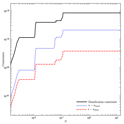
Figure 2: Evaluation of the overall numerical errors associated with the solution of Eqs. (65)–(71): with the same parameters as in the previous figures, we show here the levels at which Eqs. (74), (78) and (73) are satisfied. The most error-prone situation, at the end of the calculation, still satisfies the constraints to better than $10^{-18}$.

Fig. 3 shows the behavior of the fluid variables with $N$ around the radiation to matter transition, i.e. with the state parameter $w$ smoothly varying from its initial value of $\frac{1}{3}$ to zero. The rescaled number density $x$ is found to be negligible throughout, even though its contribution to the energy density eventually dominates. The rescaled entropy $y$ provides, roughly, all of the energy density $\rho$ initially and for most of the transition, but eventually becomes negligible, as expected. Finally, the temperature $\tilde{T}$ is seen to decay to zero, while the rescaled chemical potential $\tilde{\mu}$ asymptotically takes its fiducial value unity.

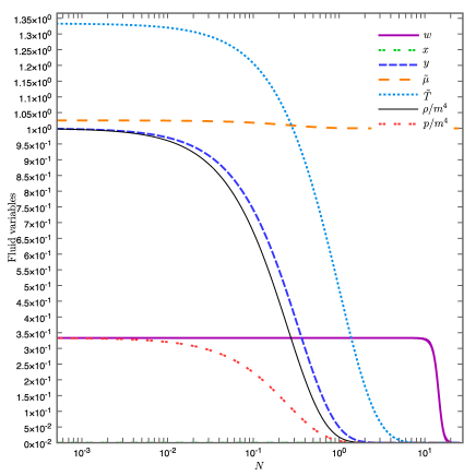
Figure 3: Background fields for the same parameters as Fig. 1.  The thick solid line corresponds to the state parameter $w$, i.e. the ratio of $\rho$ (thin full line) and $p=\Psi$ (thick double-dotted line), the number density $x\propto n$ is essentially negligible at these scales, while the density $\rho$ is dominated by the contribution of the entropy $y\propto s$ (thick dashed line); the conjugate variables, namely the rescaled temperature $\tilde{T}$ (thick dotted line) and matter chemical potential $\tilde{\mu}$ (thick long dashed line) both decrease, with $\tilde{\mu}\to 1$ as expected.

The behavior of the metric and the shears are displayed in Figs. 4 and 5, respectively. The beta coefficients change from being initially equal to each other (zero in the numerical calculation), to final constant values. With a rescaling of the spatial coordinates we can absorb these constants so as to return to the usual FLRW metric. Here we use the same parameters as before, except that we have taken $\tilde{\tau}=1,10$. The reason is illustrated in Fig. 5, which shows that the shears $\sigma_{\aleph}$, initially vanishing (because we start with a FLRW radiation dominated phase), increase first during the transition, reach a maximum and eventually decrease to vanishingly small values, which is expected for the final FLRW matter dominated epoch. As one might expect, as the coupling $\tilde{\tau}$ is increased, the anisotropies increase.

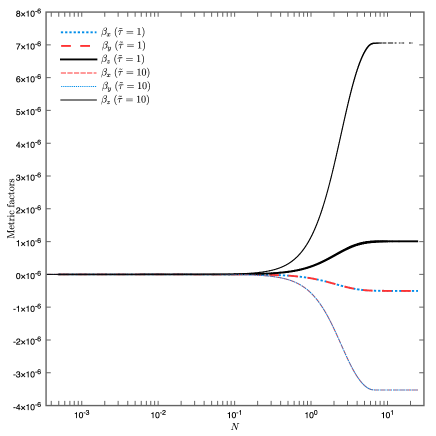
Figure 4: Metric coefficients $\beta_{i}$ as functions of the e-fold number $N$, for the same parameters as Fig. 1, except that $\tilde{\tau}=1,10$. The full thick line represents $\beta_{z}$, while the other two (dotted and dashed lines) stand for $\beta_{x}$ and $\beta_{y}$ respectively, satisfying $\beta_{x}=\beta_{y}=-\frac{1}{2}\beta_{z}$, in agreement with our setting.

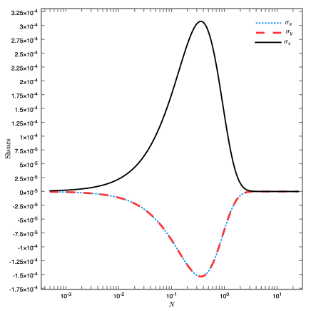
Figure 5: Shear functions $\sigma_{i}$ as functions of the e-fold number $N$, for the same parameters as Fig. 1, except that $\tilde{\tau}=1,10$. The full thick line represents $\sigma_{z}$, while the other two (dotted and dashed lines) stand for $\sigma_{x}$ and $\sigma_{y}$ respectively. Because of the relation between the metric coefficients $\beta_{i}$, it turns out that the shears satisfy a similar relation, namely $\sigma_{x}=\sigma_{y}=-\frac{1}{2}\sigma_{z}$. We also see that the anistropies increase as the coupling $\tilde{\tau}$ is increased.

Finally, Fig. 6 shows the time evolution of the sound speeds $c^{2}_{\mathrm{n}}$ and $c^{2}_{\mathrm{s}}$, as well as $\mathcal{C}_{\mathrm{n}\mathrm{s}}$ and $\mathcal{C}_{\mathrm{s}\mathrm{n}}$. We find that $c^{2}_{\mathrm{s}}=1/3$ throughout, although $c^{2}_{\mathrm{n}}$ is modified in the radiation era. Both cross-coupling terms decrease with time. This, along with the vanishing of the relative flow, is an important result for a two-stream instability analysis, for it implies that the conditions for instability are naturally eliminated by the overall expansion of the universe.

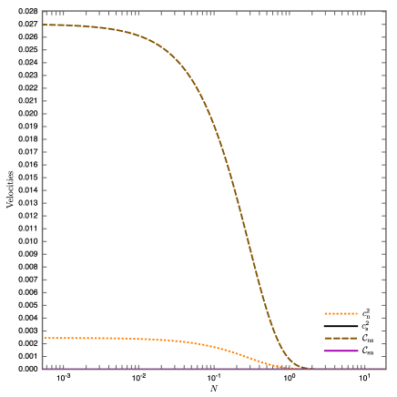
Figure 6: The bare sound speeds $c^{2}_{\mathrm{n}}$, $c^{2}_{\mathrm{s}}$, and cross-constituent couplings $\mathcal{C}_{\mathrm{n}\mathrm{s}}$ and $\mathcal{C}_{\mathrm{s}\mathrm{n}}$ as functions of the e-fold number $N$, for the same parameters as Fig. 1. Since $c^{2}_{\mathrm{s}}=1/3$ throughout, it is not shown in the figure. Both $c^{2}_{\mathrm{n}}$ (dotted line) and $\mathcal{C}_{\mathrm{n}\mathrm{s}}$ (dashed line) are smoothly decaying functions of time, while $\mathcal{C}_{\mathrm{s}\mathrm{n}}$ (full line, hardly visible on the figure) is essentially negligible at all times.

With the solution at hand, it is now possible to return to the original equations and understand what is taking place during the transition. Originally, we set initial conditions in the radiation era, for which $Ts\gg\mu n$, with the extra requirement that $V_{\mathrm{s}}\ll 1$: this means that the evolution of the three Hubble functions, and hence of the scale factors, will be identical, so the shears vanish and we are in a FLRW phase. Then, as the product $\mu n$ begins to grow, with $Ts$ decreasing, the matter velocity, provided it was large enough to begin with (and we see numerically that we need to set it very close to unity in order to have a visible effect) is still large enough that the corresponding term becomes important and the scale factors begin to evolve in different ways. Finally, even this velocity becomes sufficiently small with respect to unity that one recovers the FLRW symmetry expected for the matter dominated epoch. As to why the matter velocity can be large, and yet the universe be radiation dominated, is because it is the flux that enters the Einstein equations; a large velocity can be compensated for by a small number density.

V Closing Remarks

A main goal of this work was to develop for cosmology the general relativistic, multi-fluid model (derived from a variational formalism) that has so far been used mostly for neutron star astrophysics. While we considered only a two-fluid system, the formalism itself can, in principle, handle a number of different fluids. As it comes from an action, coupling to other fields can be imposed in more or less standard ways. For example, electromagnetism can be incorporated via the usual gauge coupling, thus allowing for plasmas and their effects on the system. We also demonstrated how relativistic condensates follow automatically because the formalism is written in terms of the conjugate momenta, and simply setting the momenta to be gradients of scalars automatically insures zero vorticity.

The two-fluid model we introduced is valid for applications in cosmology. Even though the relative motions were anti-aligned, the model illustrated behavior that one might expect from a close examination of the radiation-to-matter transition. The main task was to build a model in which both the radiation and the matter dominated eras were describable by means of an FLRW metric, as necessary to fit nucleosynthesis, CMB, and large scale structure formation data Komatsu et al. (2011); Percival et al. (2010). We found that such a situation could easily be implemented, provided the relative fluid velocity is large enough at the transition time, an assumption that needs to be justified on the basis of primordial cosmology models. Indeed, in the now well-established framework of inflation Lemoine et al. (2008), it is tremendously difficult for the Universe to remain with any relevant amount of left-over anisotropy: in fact, inflation was precisely invented to, among its expected outsets, remove any primordial anisotropy!

It should be recalled at this point that the model presented above is the simplest set-up of what might be envisioned for the transition itself, for we have not taken into account, for example, the non-conservation of the photon number through its coupling with luminous matter, matter flows with more than one constituent, or relative flows at arbitrary angles. Obviously, one would not be too surprised if comparison to observational data indicated the need for a more elaborate model. Note also that we have assumed here the matter fluid to have only one flux-component. This may not be a reasonable assumption; it is, however, largely a scale-dependent statement.

There are not so many ways to produce such primordial anisotropy. Among the most natural are perhaps models based on some amount of non trivial electromagnetic phenomena taking place during very early epochs. Consistent with large scale astrophysical observations of $\gamma-$ray halos around active galactic nuclei Ando and Kusenko (2010), the existence of relatively intense intergalactic magnetic fields of the order of $10^{-15}$ G have been deduced, whose formation is expected to be of primordial origin. Some inflationary models Anber and Sorbo (2006) are able to produce such large scale magnetic fields, that are statistically isotropic. It requires a special effort to construct a so-called “hairy” universe Watanabe et al. (2009) in which the resulting magnetic field (or any other gauge field coherent over large distances) points to a privileged spatial direction; off-diagonal $TB$ and $EB$ spectra could be induced by such models Watanabe et al. (2011), hence providing an observational means to validate them.

A special spatial direction can also exist in more radical scenarios. In one such model, for instance, a planar domain wall remains all through the inflation phase, thereby breaking the rotational invariance of the final perturbation power spectrum Wang et al. (2011). Multifield inflation can also serve that purpose by producing vorticity, although at second order in the relevant perturbations Christopherson et al. (2009).

Another way to induce a non FLRW universe (perhaps the simplest) is to start with a theory having a built-in privileged timelike vector with which the dominant fluid may not necessarily align; examples are provided by the Hořava–Lifshitz setup Hořava (2009); Blas et al. (2010), originally aimed at renormalizing gravity, and the Einstein-æther theory Jacobson (2007). Depending on the initial conditions, their solution can actually also relax to the usual FLRW solution, the fluid unit vector then aligning dynamically with the æther vector Donnelly and Jacobson (2010); Carruthers and Jacobson (2011).

In all these situations, it remains to be seen whether some cosmological variables might take values that differ from their canonical ones, as derived in the framework of the best-fit vanilla single field inflation paradigm. To clarify the situation, a full perturbation theory should now be examined Zlosnik (2011). Unlike those that assume only a single fluid, a perturbation analysis of a two-fluid system has to take into account the possibility of two-stream instability Samuelsson et al. (2010).

Such instabilities are well-established in plasma physics, and have also been argued for in laboratory superfluids and their neutron star analogs Andersson et al. (2004, 2003). Samuelsson et al. Samuelsson et al. (2010) have shown that a relative velocity and some type of coupling (cross-constituent or entrainment) for a system of two relativistic fluids is a necessary condition for two-stream instability. Roughly, there is a “window” of instability that opens when a mode appears to be, say, right-moving with respect to one of the fluids, yet left-moving with respect to the other. In this paper we have shown that the conditions for such instabilities to exist, a relative flow between two coupled fluid components, may be satisfied in cosmology. We have also shown that cosmological expansion provides a mechanism for shutting down the instability by closing the window, since both the relative velocity and the cross-constituent coupling are driven to zero.

If such instabilities were to be triggered, a basis for a set of observational constraints (or possible detections) for the transition epoch may be established. In a companion paper Comer et al. (2011), we explore whether these instabilities develop before the instability window is closed. If an instability were to develop in some of the anisotropic transitions, they would most definitely leave relevant imprints in both CMB and large scale structure data, in the form either of non-gaussianities, bizarre polarization distributions and spectra, and special scales corresponding to the Hubble volume at the transition time. For instance, it can be argued that such instabilities can occur during the matter to cosmological constant transition if and only if the latter is made of a fluid, hence having a state parameter $w>-1$; however close $w$ is to $-1$, such a fluid could initiate an instability that an actual cosmological constant, having $w=-1$, could not. Therefore, observing the relevant consequences of these instabilities at the relevant length scales would allow a discrimination between these two otherwise indistinguishable models.

Appendix: Geometric quantities

For the metric given in (4) we find the Christoffel coefficients to be

$$\Gamma^{t}_{xx} = A^{2}_{x}H_{x}\quad,\quad\Gamma^{t}_{yy}=A^{2}_{y}H_{y}\quad,\quad\Gamma^{t}_{zz}=A^{2}_{z}H_{z},$$ (90)

$$\Gamma^{x}_{tx} = H_{x}\quad,\quad\Gamma^{2}_{ty}=H_{y}\quad,\quad\Gamma^{z}_{tz}=H_{z},$$ (92)

$$\Gamma^{x}_{xz} = I_{x}\quad,\quad\Gamma^{y}_{yz}=I_{y}\quad,\quad\Gamma^{z}_{zz}=I_{z},$$ (94)

$$\Gamma^{z}_{xx} = -\left(\frac{A_{x}}{A_{z}}\right)^{2}I_{x}\quad,\quad\Gamma^{z}_{yy}=-\left(\frac{A_{y}}{A_{z}}\right)^{2}I_{y},$$ (96)

leading to the following non-vanishing components of the Ricci tensor:

$$R^{x}_{\ x} = H_{x}\sum_{\aleph}H_{\aleph}+H_{x}^{\prime}-\frac{1}{A_{z}^{2}}\left[I^{\prime}_{x}+I_{x}\left(I_{x}+I_{y}-I_{z}\right)\right],$$ (97)

$$R^{y}_{\ y} = H_{y}\sum_{\aleph}H_{\aleph}+H_{y}^{\prime}-\frac{1}{A_{z}^{2}}\left[I^{\prime}_{y}+I_{y}\left(I_{x}+I_{y}-I_{z}\right)\right],$$ (98)

$$R^{z}_{\ z} = H_{z}\sum_{\aleph}H_{\aleph}+H_{z}^{\prime}-\frac{1}{A_{z}^{2}}\left[I^{\prime}_{x}+I^{\prime}_{y}+I_{x}\left(I_{x}-I_{z}\right)+I_{y}\left(I_{y}-I_{z}\right)\right],$$ (99)

$$R^{z}_{\ t} = \frac{1}{A_{z}^{2}}\left[I_{x}\left(H_{z}-H_{x}\right)+I_{y}\left(H_{z}-H_{y}\right)-I^{\prime}_{x}-I^{\prime}_{y}\right],$$ (100)

$$R^{t}_{\ t} = \sum_{\aleph}\left(H_{\aleph}^{\prime}+H_{\aleph}^{2}\right),$$ (101)

and scalar

$$R=2\left\{\sum_{\aleph}\left(H_{\aleph}^{2}+H_{\aleph}^{\prime}\right)+H_{x}H_{y}+H_{x}H_{x}+H_{y}H_{z}-\frac{1}{A_{z}^{2}}\left[I_{x}^{\prime}+I_{y}^{\prime}+\left(I_{x}+I_{y}\right)^{2}-I_{x}I_{z}-I_{y}I_{z}-I_{x}I_{y}\right]\right\},$$ (102)

with the sign convention for the Riemann tensor given by

$$R^{\mu}_{\ \nu\alpha\beta}\equiv\partial_{\beta}\Gamma^{\mu}_{\nu\alpha}-\partial_{\alpha}\Gamma^{\mu}_{\nu\beta}+\Gamma^{\mu}_{\sigma\beta}\Gamma^{\sigma}_{\nu\alpha}-\Gamma^{\mu}_{\sigma\alpha}\Gamma^{\sigma}_{\nu\beta}.$$ (103)

From these, one can obtain the Einstein tensor (13). As pointed out in the main text, the Einstein equations are not all independent.

References

- Peter and Uzan (2009) P. Peter and J.-P. Uzan, Primordial cosmology (Oxford Graduate Texts, Oxford University press, UK, 2009).
- Modak (1984) B. Modak, J. Astrop. Astr. 5, 317 (1984).
- Triginer and Pavon (1995) J. Triginer and D. Pavon, Class. Quant. Grav. 12, 689 (1995).
- Andersson and Lopez-Monsalvo (2011) N. Andersson and C. S. Lopez-Monsalvo, Classical and Quantum Gravity 28, 195023 (2011).
- Weinberg (1971) S. Weinberg, Astrophys. J. 168, 175 (1971).
- Patel and Koppar (1991) L. K. Patel and S. S. Koppar, Australian Mathematical Society Journal Series B – Applied Mathematics 33, 77 (1991).
- Velten and Schwarz (2011) H. Velten and D. J. Schwarz, JCAP 1109, 016 (2011).
- Sikivie and Yang (2009) P. Sikivie and Q. Yang, Physical Review Letters 103, 111301 (2009).
- Harko (2011) T. Harko, Phys. Rev. D 83, 123515 (2011).
- Carter (1989) B. Carter, in Relativistic Fluid Dynamics (Noto, 1987), edited by A. Anile and M. Choquet-Bruhat (Springer-Verlag, Heidelberg, Germany, 1989), vol. 1385 of Lect. Notes Math., pp. 1–64.
- Andersson and Comer (2007) N. Andersson and G. L. Comer, Living Reviews in Relativity 10, 1 (2007).
- Nakar et al. (2011) E. Nakar, A. Bret, and M. Milosavljević, Astrophys. J. 738, 93 (2011).
- Gromov et al. (2004) A. Gromov, Y. Baryshev, and P. Teerikorpi, Astron. Astrophys. 415, 813 (2004).
- Emir Gümrükçüoglu et al. (2007) A. Emir Gümrükçüoglu, C. R. Contaldi, and M. Peloso, JCAP 11, 5 (2007).
- Pitrou et al. (2008) C. Pitrou, T. S. Pereira, and J.-P. Uzan, JCAP 4, 4 (2008).
- Kim and Minamitsuji (2010) H.-C. Kim and M. Minamitsuji, Phys. Rev. D 81, 083517 (2010).
- Dechant et al. (2009) P.-P. Dechant, A. N. Lasenby, and M. P. Hobson, Phys. Rev. D 79, 043524 (2009).
- Dey and Paban (2011) A. Dey and S. Paban, ArXiv e-prints (2011).
- Sandin (2009) P. Sandin, General Relativity and Gravitation 41, 2707 (2009).
- Harko and Lobo (2011) T. Harko and F. S. N. Lobo, Phys. Rev. D 83, 124051 (2011).
- Calogero and Heinzle (2011) S. Calogero and J. M. Heinzle, Physica 240, 636 (2011).
- Tsagas et al. (2008) C. G. Tsagas, A. Challinor, and R. Maartens, Phys. Rep. 465, 61 (2008).
- Barrow and Tsagas (2007) J. D. Barrow and C. G. Tsagas, Classical and Quantum Gravity 24, 1023 (2007).
- Adhav et al. (2011) K. S. Adhav, S. M. Borikar, M. S. Desale, and R. B. Raut, EJTP 8, 319 (2011).
- Cataldo et al. (2011) M. Cataldo, F. Arévalo, and P. Mella, Astrophys. Space Sci. 333, 287 (2011).
- Schwarz et al. (2004) D. J. Schwarz, G. D. Starkman, D. Huterer, and C. J. Copi, Physical Review Letters 93, 221301 (2004).
- Copi et al. (2010) C. J. Copi, D. Huterer, D. J. Schwarz, and G. D. Starkman, Advances in Astronomy 2010, 847541 (2010).
- Perivolaropoulos (2011) L. Perivolaropoulos, ArXiv e-prints (2011).
- Ma et al. (2011) Y.-Z. Ma, G. Efstathiou, and A. Challinor, Phys. Rev. D 83, 083005 (2011).
- Pontzen and Challinor (2007) A. Pontzen and A. Challinor, MNRAS 380, 1387 (2007).
- Pontzen (2009) A. Pontzen, Phys. Rev. D 79, 103518 (2009).
- Fixsen and Kashlinsky (2011) D. J. Fixsen and A. Kashlinsky, Astrophys. J. 734, 61 (2011).
- Komatsu et al. (2011) E. Komatsu et al., Astrophys. J. Suppl. 192, 18 (2011).
- Percival et al. (2010) W. J. Percival, B. A. Reid, D. J. Eisenstein, N. A. Bahcall, T. Budavari, J. A. Frieman, M. Fukugita, J. E. Gunn, Ž. Ivezić, G. R. Knapp, et al., MNRAS 401, 2148 (2010).
- Samuelsson et al. (2010) L. Samuelsson, C. S. Lopez-Monsalvo, N. Andersson, and G. L. Comer, General Relativity and Gravitation 42, 413 (2010).
- Comer et al. (2011) G. L. Comer, P. Peter, and N. Andersson, to be submitted (2011).
- Comer and Joynt (2003) G. L. Comer and R. Joynt, Phys. Rev. D 68, 023002 (2003).
- Lemoine et al. (2008) M. Lemoine, J. Martin, and P. Peter, eds., Inflationary Cosmology, vol. 738 (2008).
- Ando and Kusenko (2010) S. Ando and A. Kusenko, Ap. J. Lett. 722, L39 (2010).
- Anber and Sorbo (2006) M. M. Anber and L. Sorbo, JCAP 10, 18 (2006).
- Watanabe et al. (2009) M.-A. Watanabe, S. Kanno, and J. Soda, Physical Review Letters 102, 191302 (2009).
- Watanabe et al. (2011) M.-A. Watanabe, S. Kanno, and J. Soda, MNRAS 412, L83 (2011).
- Wang et al. (2011) C.-H. Wang, Y.-H. Wu, and S. D. H. Hsu, ArXiv e-prints (2011).
- Christopherson et al. (2009) A. J. Christopherson, K. A. Malik, and D. R. Matravers, Phys. Rev. D 79, 123523 (2009).
- Hořava (2009) P. Hořava, Phys. Rev. D 79, 084008 (2009).
- Blas et al. (2010) D. Blas, O. Pujolàs, and S. Sibiryakov, Phys. Rev. Lett. 104, 181302 (2010).
- Jacobson (2007) T. Jacobson, PoS QG-PH, 020 (2007).
- Jacobson (2010) T. Jacobson, Phys.Rev. D81, 101502 (2010).
- Donnelly and Jacobson (2010) W. Donnelly and T. Jacobson, Phys. Rev. D 82, 064032 (2010).
- Carruthers and Jacobson (2011) I. Carruthers and T. Jacobson, Phys. Rev. D 83, 024034 (2011).
- Zlosnik (2011) T. G. Zlosnik, ArXiv e-prints (2011).
- Andersson et al. (2004) N. Andersson, G. L. Comer, and R. Prix, Mon. Not. R. Astro. Soc. 354, 101 (2004).
- Andersson et al. (2003) N. Andersson, G. L. Comer, and R. Prix, Phys. Rev. Lett. 90, 091101 (2003).