The TW Hya Disk at 870 $\mu$m: Comparison of CO and Dust Radial Structures

Abstract

We present high resolution ($0\farcs 3=16$ AU), high signal-to-noise ratio Submillimeter Array observations of the 870 $\mu$m (345 GHz) continuum and CO $J$=3$-$2 line emission from the protoplanetary disk around TW Hya. Using continuum and line radiative transfer calculations, those data and the multiwavelength spectral energy distribution are analyzed together in the context of simple two-dimensional parametric disk structure models. Under the assumptions of a radially invariant dust population and (vertically integrated) gas-to-dust mass ratio, we are unable to simultaneously reproduce the CO and dust observations with model structures that employ either a single, distinct outer boundary or a smooth (exponential) taper at large radii. Instead, we find that the distribution of millimeter-sized dust grains in the TW Hya disk has a relatively sharp edge near 60 AU, contrary to the CO emission (and optical/infrared scattered light) that extends to a much larger radius of at least 215 AU. We discuss some possible explanations for the observed radial distribution of millimeter-sized dust grains and the apparent CO-dust size discrepancy, and suggest that they may be hallmarks of substructure in the dust disk or natural signatures of the growth and radial drift of solids that might be expected for disks around older pre-main sequence stars like TW Hya.

1 Introduction

The physical conditions of the gas and dust in young circumstellar disks shape the formation and early evolution of planetary systems. The spatial distribution of disk material – the density structure – plays many fundamental roles, and is especially relevant for dictating when and where planets can form and migrate in the disk. Naturally, empirical constraints on protoplanetary disk structures are of significant value in efforts to develop realistic models of the complex processes involved in planet formation. Some recent studies have made progress in extracting the radial (surface) density profiles in these disks from high angular resolution measurements of their millimeter-wave continuum emission (Andrews et al., 2009, 2010b; Isella et al., 2009; Guilloteau et al., 2011). However, such observations are only sensitive to the density structure of the (presumably) trace population of disk solids, and not the gas that wields far more influence over the evolution of disk structure and the formation of planets. The major challenge is that the gas in these disks is primarily cold H₂, which is not directly observable. And while there have been many investigations of less abundant molecular species (see Dutrey et al., 2007), limited sensitivity to low optical depth lines and an incomplete understanding of the complicated chemistry in these disks have so far made it difficult to convert observations of the gas into density constraints (see Williams & Cieza, 2011).

Given those obstacles, there have not been many attempts to directly compare the gas and dust structures of protoplanetary disks with spatially resolved data. A few studies used simple models to fit the millimeter continuum (dust) and CO line (gas) emission independently, finding inconsistent structures where the dust is much more compact than the gas (Piétu et al., 2005; Isella et al., 2007). Hughes et al. (2008) suggested that this discrepancy was likely an optical depth illusion, an artifact of the assumed sharp outer edge in the density model. They showed that a surface density profile with a smooth taper at large radii could better reproduce the dust and gas observations. However, Panić et al. (2009) argued that similar modifications to the model structure of the IM Lup disk (see Pinte et al., 2008) were insufficient to account for the much different sizes they measure for its gas and dust emission. Recently, Qi et al. (2011) successfully matched their observations of multiple CO transitions and continuum emission from the HD 163296 disk with a single density model, although refinements to that model based on the detailed morphology of the continuum emission were not a priority in that study. In general, there is still substantial uncertainty that the gas and dust trace the same structures in protoplanetary disks. From a practical standpoint, that uncertainty is disconcerting. Our knowledge of the mass contents of these disks is entirely based on their (easy to measure) dust emission, but we are not sure if those dust structures also describe the gas reservoirs that effectively control the key disk evolution and planet formation processes.

Although direct measurements of H₂ densities are not possible, in principle an indirect comparison of the dust and gas structures in a protoplanetary disk can be made with sufficiently sensitive and high resolution observations of the thermal continuum and emission lines from trace gas species. To meet those requirements, a relatively massive and nearby disk would be an ideal candidate target. TW Hya is an isolated, $\sim$0.8 M_⊙ T Tauri star located only $54\pm 6$ pc from the Sun (Rucinski & Krautter, 1983; Wichmann et al., 1998; van Leeuwen, 2007). Despite its advanced age ($\sim$10 Myr; Kastner et al., 1997; Webb et al., 1999), it hosts a massive, gaseous accretion disk with a rich molecular spectrum and strong continuum emission out to centimeter wavelengths (Wilner et al., 2000, 2003, 2005; Qi et al., 2004, 2006, 2008). Those observations and a suite of resolved optical/infrared scattered light images confirm that the disk is well-resolved and viewed nearly face-on (Krist et al., 2000; Trilling et al., 2001; Weinberger et al., 2002; Apai et al., 2004; Roberge et al., 2005). The inner edge of this “transition” disk is truncated at a radius of 4 AU, likely by an unseen (and maybe planetary) companion (Calvet et al., 2002; Hughes et al., 2007). Given its proximity, favorable orientation, and rich gas and dust content, the TW Hya disk is uniquely well-suited for a comparative investigation of the radial behavior of its gas and dust structures.

In this article, we present new sub-arcsecond resolution observations of the 870 $\mu$m continuum and CO $J$=3$-$2 emission from the TW Hya disk. Using state-of-the-art radiative transfer modeling tools, we use those measurements to compare the radial distributions of its CO gas and dust. In §2 we describe the observations and data calibration. The basic characteristics of the data are reviewed in §3. A detailed description of the modeling and results are provided in §4. The implications of that analysis are discussed in §5, and our principle conclusions are summarized in §6.

2 Observations and Data Reduction

TW Hya was observed at 345 GHz (870 $\mu$m) with the Submillimeter Array (SMA; Ho et al., 2004) on 8 occasions in 2006-2010 in the compact (C), extended (E), and very extended (V) array configurations, providing baseline lengths of 16-70 m, 28-226 m, and 68-509 m, respectively. To accomodate various studies of the CO $J$=3$-$2 emission line (at 345.796 GHz), the SMA double sideband receivers and correlator were configured with several different local oscillator (LO) settings and spectral resolutions throughout this campaign. The “default” setup used an LO frequency of 340.755 GHz (880 $\mu$m) with the CO line in the center of the upper sideband, with a resolution of 0.70 km s^-1 in one spectral chunk. The other 23 partially-overlapping 104 MHz spectral chunks in each sideband were sampled coarsely with 32 channels each. Some of the 2008 observations utilized a “high” resolution correlator mode, with a large portion of the bandwidth devoted to probing the CO line with 0.044 km s^-1 channels (see Hughes et al., 2011). While those data sample the continuum with the default spectral resolution, they have a reduced continuum bandwidth (2.6 GHz; $\sim$70% of the available bandwidth at the time) and a higher LO frequency at 349.935 GHz (857 $\mu$m). The 2010 observations were conducted in a “medium” resolution mode that employed the new expanded bandwidth capabilities at the SMA. In that case, two different 2 GHz IF bands were centered $\pm$5 GHz (the normal setup) and $\pm$7 GHz from the LO frequency, 339.853 GHz (883 $\mu$m). The CO line was observed at a moderate resolution of 0.18 km s^-1 in the upper sideband of the first IF band, and the continuum was coarsely sampled across the remaining expanded bandwidth. Finally, a “hybrid” mode was utilized at the end of 2006 to cover the $J$=4$-$3 transition of H¹³CO⁺ (see Qi et al., 2008). A summary of the observational setups is provided in Table 1.

Table 1: Summary of SMA Observations

UT Date	array	spectral	RMS noise	beam size	beam PA
	config.	setup	[mJy beam-1]	[″]	[°]
(1)	(2)	(3)	(4)	(5)	(6)
2006 Dec 28	C	hybrid	3.7	$4.2\times 1.7$	4
2008 Jan 23	E	high	3.2	$0.9\times 0.7$	21
2008 Feb 20	E	high	3.1	$1.0\times 0.7$	$-$20
2008 Feb 21	E	default	4.1	$1.2\times 0.5$	14
2008 Mar 2	C	high	3.6	$3.9\times 1.9$	$-$17
2008 Mar 9	C	default	3.2	$3.7\times 1.8$	$-$13
2008 Apr 3	V	default	2.2	$0.6\times 0.3$	19
2010 Feb 9	V	medium	1.8	$0.5\times 0.3$	$-$3
combined	all	$\cdots$	2.0	$0.8\times 0.6$	$-$3

Note. — Col. (1): UT date of observations. Col. (2): SMA array configuration, C = compact, E = extended, and V = very extended. Col. (3): Adopted correlator mode (see §2). Col. (4): Continuum RMS noise in a naturally-weighted map. Col. (5): Naturally-weighted synthesized beam dimensions. Col. (6): Naturally-weighted synthesized beam orientation (major axis position angle, measured east of north).

TW Hya was observed in an alternating sequence with the nearby quasar J1037-295 (a projected separation of 7.3°), with a total cycle time of 15 minutes in the C and E configurations and 8-10 minutes in the V configuration. The quasars 3C 279 or J1146-289 were observed every other cycle. For the tracks on 2008 February 21, March 9, and April 3, the target portion of the cycle was shared with the nearby sources HD 98800 and Hen 3-600 (see Andrews et al., 2010a). Planets, satellites, and bright quasars were observed as bandpass and absolute flux calibrators when TW Hya was at low elevations ($<$18°), depending on their availability and the array configuration. Most of these data were obtained in the best atmospheric conditions available at Mauna Kea, with zenith opacities of 0.03-0.05 at 225 GHz (0.6-1.0 mm of precipitable water vapor) and well-behaved phase variations on timescales longer than the calibration cycle. The conditions on 2008 March 2 and 9 were worse, but typical for Mauna Kea (with 1.4-1.8 mm of precipitable water vapor).

The data from each individual observation were reduced independently with the IDL-based MIR software package. The bandpass response was calibrated with observations of bright planets and quasars, and broadband continuum channels in each sideband (and IF band, where applicable) were generated by averaging and then combining the central 82 MHz in each line-free spectral chunk. The visibility amplitude scale was derived from observations of Uranus, Titan, Callisto, or Vesta, with a typical systematic uncertainty of 10-15%. The antenna-based complex gain response of the system was determined with reference to J1037-295. The observations of 3C 279 or J1146-289 were used to assess the quality of phase transfer in the gain calibration process. Based on those data, we estimate that the “seeing” generated by atmospheric phase noise and any small baseline errors is small, 0.10-0$\farcs$15. This result is a testament to the high quality of the observing conditions, especially given the low target elevation and wide projected separations between the calibrators (for reference, 3C 279 is located 39.7° from TW Hya and 38.5° from J1037-295, while the corresponding separations for J1146-289 are 11.0° and 15.1°, respectively).

Before the observations could be combined, we had to account for the proper motion of TW Hya over the $\sim$3 year observing baseline ($\mu_{\alpha}\cos{\delta}=-0\farcs 066$ yr^-1, $\mu_{\delta}=-0\farcs 014$ yr^-1; van Leeuwen, 2007). Fortunately, each individual dataset exhibited bright, symmetric, centrally-peaked continuum emission that we associate with dust in the TW Hya disk. Using elliptical Gaussian fits to those continuum visibilities, we determined centroid positions for each individual set of observations and associated them with the stellar position at that epoch. The measured emission centroids are consistent with the expected stellar positions, well within the $\sim$0$\farcs$1 absolute astrometric accuracy of the SMA (set primarily by small baseline uncertainties). Based on those centroid measurements, each individual dataset was aligned to a common coordinate system. After confirming that the aligned visibility sets showed excellent agreement on all overlapping baselines, all datasets were combined to produce composite 345 GHz continuum and CO $J$=3$-$2 visibilities.

The composite visibilities were Fourier inverted, deconvolved with the CLEAN algorithm, and restored with a synthesized beam using the MIRIAD software package. The natural weighting of the continuum data produces an image with a $0\farcs 80\times 0\farcs 58$ beam and an RMS noise level of 2.0 mJy beam^-1 (which is dynamic-range limited). Composite CO $J$=3$-$2 channel maps were synthesized with a velocity resolution of 0.2 km s^-1 and a circular beam with a FWHM of 1$\farcs$0 (the naturally-weighted resolution is $0\farcs 96\times 0\farcs 73$). The RMS noise level is 0.13 Jy beam^-1 in each channel.

Ancillary information in the literature was used to construct the TW Hya spectral energy distribution (SED) that will be used with the SMA data. We adopted the optical monitoring results of Mekkaden (1998) and near-infrared photometry from Weintraub et al. (2000) and the 2MASS point source catalog (Cutri et al., 2003). In the thermal infrared, Spitzer flux densities measured by Hartmann et al. (2005) and Low et al. (2005) were supplemented with IRAS and Herschel data (Weaver & Jones, 1992; Thi et al., 2010). We also include a Spitzer IRS spectrum, kindly provided by E. Furlan (see Uchida et al., 2004). At submillimeter wavelengths, we relied on the calibrator flux densities from the SHARC-II and SCUBA instruments at the Caltech Submillimeter Observatory and James Clerk Maxwell Telescope, respectively ($F_{\nu}=6.13\pm 0.68$, $3.9\pm 0.7$, and $1.37\pm 0.01$ Jy at 350, 443, and 869 $\mu$m, respectively). Additional millimeter-wave measurements were collected from Weintraub et al. (1989), Qi et al. (2004), and Wilner et al. (2003).

3 Results

The astrometrically aligned and combined SMA data are shown together in Figure 1, along with the broadband SED. The synthesized continuum image in Figure 1$a$ has an effective frequency of 344.4 GHz (870 $\mu$m), with an integrated flux density of $1.34\pm 0.13$ Jy and a peak flux density of $0.337\pm 0.034$ Jy beam^-1 (a peak signal-to-noise ratio of $\sim$170), including the systematic calibration uncertainties. The continuum emission is regular and symmetric on the angular scales probed here, with a synthesized beam size of $43\times 31$ AU projected on the sky. Essentially no emission is detected outside a $\sim$1″ radius. Given that the integrated flux density determined from the SMA data is in good agreement with single-dish measurements (see §2; Weintraub et al., 1989; Di Francesco et al., 2008), it is clear that this is no optical depth effect: all of the millimeter-wave dust emission from the TW Hya disk is concentrated inside a projected radius of $\sim$60 AU.

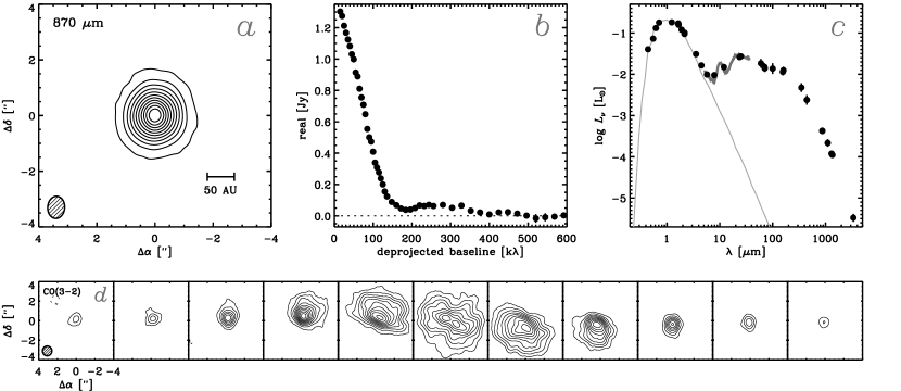
Figure 1: ($a$) Naturally weighted composite image of the 870 $\mu$m continuum emission from the TW Hya disk. Contours start at 10 mJy beam^-1 (5 $\sigma$) and increase in 30 mJy beam^-1 (15 $\sigma$) increments. The synthesized beam dimensions are shown in the lower left. ($b$) Azimuthally averaged 870 $\mu$m continuum visibility profile as a function of the deprojected baseline length (real part only; the imaginary terms are effectively zero on all baselines). The uncertainties are typically smaller than the symbol sizes. Note the low-amplitude oscillations beyond $\sim$150 k$\lambda$. ($c$) Complete SED for the TW Hya star+disk system (references are in the text; see §2). The Spitzer IRS spectrum is shown as a thick gray curve. Our adopted stellar photosphere model is overlaid as a thin gray curve (see §4.1). ($d$) CO $J$=3$-$2 channel maps from the TW Hya disk, on the same angular scale as the continuum map in panel $a$. Contours are drawn at 0.4 Jy beam^-1 intervals ($\sim$3 $\sigma$) in each 0.2 km s^-1-wide channel. The 1″ synthesized beam is shown in the lower left. The central channel represents the TW Hya systemic velocity, at $V_{\rm LSR}=+2.86$ km s^-1.

While the continuum image appears rather plain, some interesting emission features are apparent in a direct examination of the visibilities. Figure 1$b$ displays the azimuthally averaged 870 $\mu$m continuum real visibilities as a function of the deprojected baseline length (see Andrews et al., 2009), assuming the inclination ($i=6\arcdeg$) and major axis position angle (PA = 335°) derived from high spectral resolution CO emission line data by Hughes et al. (2011). The imaginary visibilities are effectively zero within the noise on all sampled baselines, confirming the accuracy of the astrometric alignment and reinforcing that there are no obvious departures from axisymmetry in the TW Hya disk. The visibility profile in Figure 1$b$ shows a smooth decrease out to $\sim$150 k$\lambda$, followed by low-amplitude oscillations on longer baselines and an apparent null near 500 k$\lambda$. These features are distinct in independent datasets (particularly the “dip” near 180 k$\lambda$, where 4 different observations span that range of baselines), are present regardless of the bin sizes used for profile averaging, and are not noted in the visibility profiles for the test calibrators (J1146-289 or 3C 279). Despite the challenges of calibrating SMA data for low-elevation targets, the persistence of these visibility modulations make us confident that they are real features. Moreover, we will demonstrate in §4 that they can be reproduced with models that incorporate a sharp outer edge in their emission profiles. The null at 500 k$\lambda$ is consistent with the 4 AU-radius inner disk cavity inferred from the SED (see Figure 1$c$; Calvet et al., 2002) and a VLA 7 mm continuum image (Hughes et al., 2007).

The panels in Figure 1$d$ show the composite CO $J$=3$-$2 emission line channel maps for the TW Hya disk, resampled to a velocity resolution of 0.2 km s^-1 with a circular 1$\farcs$0 (54 AU) synthesized beam. The emission is firmly detected ($>$3 $\sigma$) out to $\pm$1.2 km s^-1 from the systemic velocity ($V_{\rm LSR}=2.86$ km s^-1), with an integrated intensity of $34.8\pm 3.5$ Jy km s^-1 and a peak flux of $4.2\pm 0.4$ Jy beam^-1 ($43\pm 4$ K), including the calibration uncertainties. Those values are in good agreement with previous single-dish and SMA measurements (van Zadelhoff et al., 2001; Qi et al., 2004; Hughes et al., 2011). The channel maps in Figure 1$d$ show a clear rotation pattern, from northwest (blueshifted) to southeast (redshifted), with a narrow line-width due to a face-on viewing geometry. Near the systemic velocity, the CO emission subtends $\sim$4″ (215 AU) in radius.

4 Modeling Analysis

These SMA observations offer some new insights into the TW Hya disk structure. Naturally, as one of the nearest pre-main sequence stars, TW Hya and its associated disk have been the subject of intense observational scrutiny. The global structure of the TW Hya disk has been investigated previously, using the SED (Calvet et al., 2002), optical/infrared scattered light observations (Krist et al., 2000; Trilling et al., 2001; Weinberger et al., 2002; Apai et al., 2004; Roberge et al., 2005), millimeter/radio-wave continuum images (Wilner et al., 2000, 2003, 2005; Hughes et al., 2007), and resolved molecular line maps (Qi et al., 2004, 2006, 2008; Hughes et al., 2008, 2011). However, none of those previous studies had the combination of angular resolution and sensitivity for the optically thin dust and high-quality gas tracers that are available from the SMA datasets presented here.

In the following, a technique is described for extracting the structure of the TW Hya disk from these data using radiative transfer models. We focus specifically on enabling a comparison between the radial distributions of the dust and CO tracers. The approach we have adopted to make that comparison consists of three key steps. First, we construct a model of the radial density structure of the dust that is able to reproduce our resolved observations of 870 $\mu$m continuum emission and the broadband SED. Next, we make the assumption of a radially constant (vertically-integrated) dust-to-gas mass ratio and use the model structure we derive from the dust to predict the emission morphology of the CO $J$=3$-$2 line. Then, we show that this assumption implies an inconsistency with the observations, highlighting a clear difference in the radial distributions of millimeter-sized dust grains and CO gas in the TW Hya disk. Some of the potential implications of this inconsistency are discussed further in §5.

4.1 Dust Structure

The dust disk structure is determined following the technique outlined by Andrews et al. (2011), with some modifications for generality. We assume the dust is spatially distributed with a parametric two-dimensional density structure in cylindrical-polar coordinates {$r$, $z$},

$$\rho_{d}(r,z)=\frac{\Sigma_{d}}{\sqrt{2\pi}z_{d}}\exp{\left[-\frac{1}{2}\left(\frac{z}{z_{d}}\right)^{2}\right]},$$ (1)

where $\Sigma_{d}$ and $z_{d}$ are surface densities and characteric heights, which both vary radially (see below). As will be explained further in §4.3, we investigated two different models for the radial surface density profile. First, we employed the similarity solution for simple viscous accretion disk structures (Lynden-Bell & Pringle, 1974) that we have used successfully to characterize both normal and transition disks in the past (Andrews et al., 2009, 2010a, 2010b, 2011; Hughes et al., 2010). In that case,

$$\Sigma_{d}(r)=\Sigma_{c}\left(\frac{r}{r_{c}}\right)^{-\gamma}\exp{\left[-\left(\frac{r}{r_{c}}\right)^{2-\gamma}\right]},$$ (2)

where $\Sigma_{c}$ is a normalization, $r_{c}$ is a characteristic scaling radius, and $\gamma$ is a gradient parameter. As an alternative, we considered a less physically motivated (but perhaps more commonly used) model that incorporates a power-law density profile with a sharp cut-off (see Andrews et al., 2008),

$$\Sigma_{d}(r)=\Sigma_{0}\left(\frac{r}{r_{0}}\right)^{-p}\,\,\,\,\,\,\,({\rm if}\,\,\,r\leq r_{0};\,\,{\rm else}\,\,\,\Sigma_{d}=0),$$ (3)

where $\Sigma_{0}$ is a normalization, $r_{0}$ is the outer edge of the disk, and $p$ is a gradient parameter. In either case, the surface densities at small radii are modified to account for the TW Hya disk cavity (Calvet et al., 2002; Hughes et al., 2007). To simplify the inner disk model of Andrews et al. (2011), we set the surface densities to a constant value $\Sigma_{\rm in}$ between the sublimation radius ($r_{\rm sub}$) and a “gap” radius ($r_{\rm gap}$). No dust is present between that gap radius and the cavity edge, $r_{\rm cav}$. In the vertical dimension, the dust is distributed like a Gaussian with a variance $z_{d}^{2}$. The characteristic height varies with radius like $z_{d}=z_{0}(r/r_{0})^{1+\psi}$. Following Andrews et al. (2011), we employ a cavity “wall” to reproduce the infrared spectrum of TW Hya (no such feature was required at the sublimation radius). The local value of $z_{d}$ is scaled up to $z_{\rm wall}$ at $r_{\rm cav}$, and then exponentially joined to the global $z_{d}$ distribution over a small radial width, $\Delta r_{\rm wall}$.

This structure model has 11 parameters: three describe the base surface density profile, {$\Sigma_{c}$, $r_{c}$, $\gamma$} or {$\Sigma_{0}$, $r_{0}$, $p$}, five determine the cavity and inner disk properties, {$\Sigma_{\rm in}$, $r_{\rm sub}$, $r_{\rm gap}$, $r_{\rm cav}$, $\Delta r_{\rm wall}$}, and three others characterize the vertical distribution of dust, {$z_{0}$, $z_{\rm wall}$, $\psi$}. To simplify the modeling, we fixed some of the parameters that are of less direct interest here. The sublimation radius was set to $r_{\rm sub}=0.05$ AU, the location where dust temperatures reach 1400 K (see also Eisner et al., 2006). The gap radius was set to $r_{\rm gap}=0.3$ AU and the (constant) inner disk density to $\Sigma_{\rm in}=5\times 10^{-4}$ g cm^-2. The cavity edge was fixed at $r_{\rm cav}=4$ AU (see Hughes et al., 2007), the wall height was set to $z_{\rm wall}=0.25$ AU, and the wall width to $\Delta r_{\rm wall}=1$ AU. Since the details of this gap are not the focus, no attempt was made to reconcile the models with infrared interferometric data (but see Eisner et al., 2006; Ratzka et al., 2007; Akeson et al., 2011). After extensive experimentation with modeling the SED, we also fixed the scale height gradient to $\psi=0.25$. The interplay and degeneracies between these free parameters were discussed in detail by Andrews et al. (2011). For our purposes here, it is worth emphasizing that the parameters we have fixed have little quantitative impact on the derived radial structures (i.e., sizes and density gradients).

We used the dust composition advocated by Pollack et al. (1994), consisting of a mixture of astronomical silicates, water ice, troilite, and organics with the abundances, optical properties, and sublimation temperatures discussed by D’Alessio et al. (2001). Based on the efforts of Uchida et al. (2004) to faithfully reproduce the details of the Spitzer IRS spectrum, we let 25% of the total silicate abundance inside the disk cavity ($r\leq r_{\rm cav}$) be composed of crystalline forsterite (using optical constants from Jäger et al., 2003). Two grain populations were employed, with a power-law size ($s$) distribution, $n(s)\propto s^{-3.5}$, between $s_{\rm min}=0.005$ $\mu$m and a given $s_{\rm max}$. Outside the cavity wall, 95% of the dust (by mass) has $s_{\rm max}=1$ mm and the remaining 5% has $s_{\rm max}=1$ $\mu$m. The dust in the wall itself and the tenuous inner disk was assumed to have $s_{\rm max}=1$ $\mu$m. No effort was made to distinguish the vertical distributions of these dust populations. Opacity spectra for each population were determined from Mie calculations, assuming segregated spherical grains. For these dust assumptions, the 870 $\mu$m dust opacity in the outer disk is $\kappa_{\rm mm}=3.4$ cm² g^-1.

We assumed the central star has a K7 spectral type with $T_{\rm eff}=4110$ K, $R_{\ast}=1.04$ R_⊙, and $M_{\ast}=0.8$ M_⊙ ($\log{g}=4.3$), based on an effort to match Lejeune et al. (1997) spectral synthesis models to the broadband SED and the detailed optical/infrared spectral analysis work of Yang et al. (2005). The best-fit stellar spectrum template is overlaid on the SED in Figure 1$d$ as a light gray curve. Recently, Vacca & Sandell (2011) have argued instead for a M2.5 spectral type in the near-infrared, and a correspondingly cooler stellar photosphere (3400 K), larger radius (1.29 R_⊙), and lower mass (0.4 M_⊙). While that stellar model provides a good match to the broadband infrared photometry for TW Hya, it underpredicts the observed optical fluxes by a factor of $\sim$3 (in the $BVR$ bandpasses, and its known variability does not bridge that gap; see Mekkaden, 1998). We prefer the parameters for the warmer photosphere because they produce a template spectrum that better matches the SED across the complete set of optical and infrared bandpasses.

For a given set of parameters, we simulated the stellar irradiation and emission output of a model dust structure using the two-dimensional, axisymmetric Monte Carlo radiative transfer code RADMC (see Dullemond & Dominik, 2004a). Assuming the fixed viewing geometry determined by Hughes et al. (2011), a raytracing algorithm was then used to compute a synthetic model SED and set of 870 $\mu$m continuum visibilities sampled at the same spatial frequencies observed with the SMA. For each surface density model, we found the best simultaneous fit to the observed SED and SMA visibilities over a coarse grid of the gradient parameter $\gamma$ or $p$, by varying the parameters {$\Sigma_{c}$ or $\Sigma_{0}$, $r_{c}$ or $r_{0}$, $z_{0}$}. Based on those results, we refined our search and permitted the gradients to vary freely to find the best-fit parameter sets for each model type (see §4.3 for results).

4.2 CO Gas Structure

Unlike for the dust, the radial density profile of the gas disk cannot be inferred directly from models of the optically thick $J$=3$-$2 transition of CO. Therefore, we make a fundamental assumption that the gas traces the dust in the radial dimension. For any given $\Sigma_{d}$, we define the gas surface density profile as $\Sigma_{g}=\Sigma_{d}/\zeta$, where $\zeta$ is a (radially) constant dust-to-gas mass ratio.

However, we have elected to permit some freedom in the vertical distribution of the gas to facilitate a more faithful reproduction of the CO channel maps. Using a multi-transition CO dataset, Qi et al. (2006) noted that models of the TW Hya disk structure had a difficult time reproducing an appropriate vertical temperature gradient of the gas. The intensity of the high-excitation $J$=6$-$5 line indicated that the gas in the disk atmosphere was significantly hotter than the dust, presumably due to substantial X-ray heating from the central star. To be able to reproduce the observed CO spectral images, we have characterized the vertical temperature profile of the gas in parametric form, based on the modeling analysis of Dartois et al. (2003). We assume that

$$T_{g}(r,z)=T_{a}+(T_{m}-T_{a})\cos{\left(\frac{\pi z}{2z_{q}}\right)}^{2\delta},$$ (4)

where $T_{a}=T_{1}(r/{\rm 1\,AU})^{-q}$ is a parametric radial temperature profile in the disk atmosphere, $T_{m}$ is the midplane temperature determined from the RADMC simulations of the dust, $\delta$ describes the shape of the vertical profile, and $z_{q}$ defines the height of the atmosphere layer such that $T_{g}(z\geq z_{q})=T_{a}$. In our modeling, we fix $\delta=2$ and $z_{q}=4H_{p}$, where $H_{p}$ is the pressure scale height assuming the midplane temperature at each radius ($H_{p}=c_{s}/\Omega$, the ratio of the midplane sound speed to the Keplerian angular velocity). In practice, Eq. (4) is a reasonable parametric approximation of the vertical temperature profile in an irradiated disk (e.g., D’Alessio et al., 1999). We have grounded the models by forcing $T_{g}=T_{d}$ at the midplane ($z=0$), but allowed the gas temperatures to increase faster with height than the dust to simulate any additional external heating sources. For a given $T_{g}(r,z)$ specified by {$T_{1}$, $q$}, we then calculate the vertical density structure of the gas by numerically integrating the equation of vertical hydrostatic equilibrium,

$$\frac{\partial\ln{\rho_{g}}}{\partial z}=-\left[\left(\frac{GM_{\ast}z}{(r^{2}+z^{2})^{3/2}}\right)\left(\frac{\mu m_{H}}{kT_{g}}\right)+\frac{\partial\ln{T_{g}}}{\partial z}\right]$$ (5)

using $\Sigma_{g}$ as a boundary condition, where $G$ is the gravitational constant, $\mu=2.37$ is the mean molecular weight of the gas, $m_{H}$ is the mass of a hydrogen atom, and $k$ is the Boltzmann constant. For reference, a vertical slice of a representative model structure is shown in Figure 2.

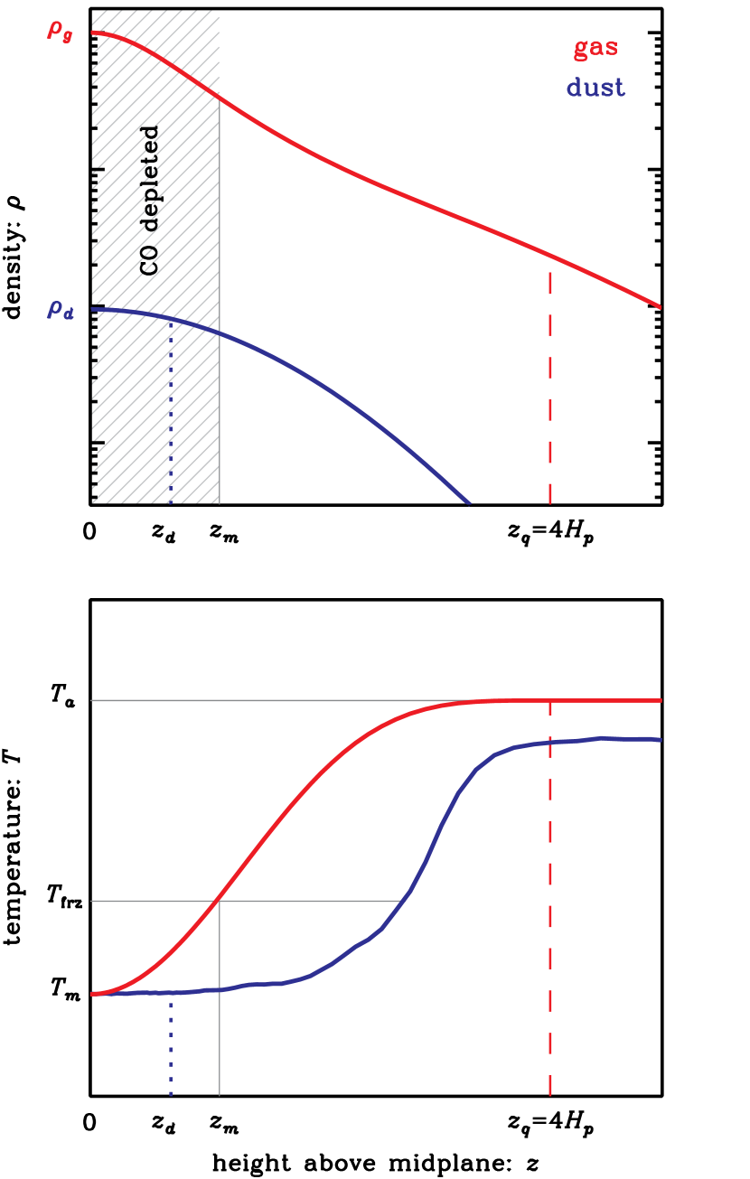
Figure 2: Schematic demonstration of our model vertical structure, shown as a vertical slice at a fixed radius. (top) The density profile of the gas (red) and dust (blue) as a function of height above the midplane. The latter has a parametric Gaussian distribution with a variance $z_{d}^{2}$, while the former is computed assuming it is in hydrostatic pressure balance for its specified temperature structure. The relative normalizations of each are represented accurately, such that $\Sigma_{d}=\zeta\Sigma_{g}$, where $\zeta$ is a fixed dust-to-gas mass ratio. The hatched region near the midplane ($z\leq z_{m}$) marks where CO is depleted from the gas phase because it is frozen onto dust grain mantles (where $T_{g}\leq T_{\rm frz}$). The comparable surface CO depletion zone due to photodissociation ($z\geq z_{s}$) is well off the right of the plot. (bottom) The corresponding temperature profiles, where $T_{d}$ is computed from the RADMC radiative transfer calculations and $T_{g}$ is determined parametrically, as described in the text. The gas and dust temperatures are equivalent ($T_{g}=T_{d}=T_{m}$) in the midplane, but $T_{g}$ rises more rapidly than the dust before it saturates to a value $T_{a}$ at a height $z_{q}$.

To quantify the density of CO molecules from any given gas model structure, we adopt the layered approach of Qi et al. (2008, 2011). Based on the detailed chemical calculations of Aikawa & Nomura (2006), we define two vertical boundaries {$z_{m}$, $z_{s}$} at any given radius such that the CO mass fraction (relative to H₂) is $X_{\rm co}$ if $z_{m}(r)\leq z\leq z_{s}(r)$ and $10^{-4}X_{\rm co}$ elsewhere. The “midplane” boundary, $z_{m}$, marks the maximum height where CO molecules are expected to be frozen out of the gas phase and affixed to dust grain mantles. In practice, $z_{m}$ is defined as the minimum height where $T_{g}\geq T_{\rm frz}$, where the freeze-out temperature $T_{\rm frz}$ is a parameter considered to be constant with radius. The “surface” boundary, $z_{s}$, is meant to represent the height where CO molecules can be photodissociated by X-rays or cosmic rays. Following Qi et al. (2008), we define $z_{s}$ such that

$$N_{\rm pd}=\frac{1}{\mu m_{H}}\int_{\infty}^{z_{s}}\rho_{g}\,\,dz,$$ (6)

where $N_{\rm pd}$ is a vertically-integrated H₂ column density that effectively represents the penetration depth of the photodissociating radiation field: $N_{\rm pd}$ is treated as a radially constant parameter.

So, for any dust model a corresponding CO model can be characterized with a set of six additional parameters: two describe the abundances of dust and CO relative to the total gas mass, {$\zeta$, $X_{\rm co}$}, two others characterize the gas temperatures in the disk atmosphere, {$T_{1}$, $q$}, and the last two define the spatial distribution of CO in the gas phase, {$T_{\rm frz}$, $N_{\rm pd}$}. For a given set of these parameters, we generate a two-dimensional grid of $n_{\rm co}(r,z)$ and $T_{g}(r,z)$ values and define a velocity field based on Keplerian rotation around a point mass $M_{\ast}$, assuming a minimal turbulent velocity line width of 10 m s^-1 based on the analysis of Hughes et al. (2011). We then feed that information into the radiative transfer modeling code LIME (Brinch & Hogerheijde, 2010) to solve the non-LTE molecular excitation conditions of the model and generate a synthetic high-resolution model cube for the CO $J$=3$-$2 transition. That model cube was then re-sampled at the velocity resolution of the data, and its Fourier transform was sampled at the same spatial frequencies observed by the SMA. In practice, we fixed the dust-to-gas ratio based on the assumed dust composition, where $\zeta=0.014$ (a gas-to-dust mass ratio of 71, see Pollack et al., 1994; D’Alessio et al., 2001). For each dust model, we varied {$T_{1}$, $q$} for a coarse grid of CO abundance layer parameters {$X_{\rm co}$, $T_{\rm frz}$, $N_{\rm pd}$} to find the best available match to the SMA spectral visibilities. Since we are using only a single CO transition in this investigation, the abundance layer parameters do not have a strong, independent effect on the synthetic CO visibilities. For simplicity, we adopt the best-fit models where $X_{\rm co}=2\times 10^{-6}$, $T_{\rm frz}=20$ K, and $N_{\rm pd}=10^{21}$ cm^-2 as representative.

Table 2: Estimated Model Parameters and Fit Results

Model	$\Sigma_{d}$(10)	$\gamma$, $p$	$r_{c}$, $r_{0}$	$z_{d}$(10)	$T_{a}$(10)	$q$	$\chi_{\rm sed}^{2}$	$\chi_{\rm cont}^{2}$	$\chi_{\rm co}^{2}$
	[g cm-2]		[AU]	[AU]	[K]
(1)	(2)	(3)	(4)	(5)	(6)	(7)	(8)	(9)	(10)
sA	0.29	1.0	35	0.62	104	0.55	201	313,914	319,974
sB	0.51	0.5	43	0.58	101	0.54	204	304,303	319,989
sC	0.28	0.0	45	0.57	98	0.54	210	302,132	320,013
sD	0.20	-0.5	42	0.53	103	0.53	216	304,329	320,024
sE	0.14	-1.0	40	0.50	102	0.53	231	307,785	320,040
pA	0.79	1.5	77	0.62	104	0.54	205	309,370	320,056
pB	0.46	1.0	67	0.60	99	0.54	211	302,747	320,047
pC	0.39	0.75	60	0.58	99	0.54	215	301,785	320,044
pD	0.31	0.5	58	0.58	100	0.54	227	302,570	320,035
pE	0.23	0.0	51	0.55	104	0.54	249	306,980	320,068

Note. — Col. (1): Model designation, where ‘s’ = similarity solution and ‘p’ = power-law with sharp edge as defined in Eq. 2 and 3, respectively. Col. (2): Dust surface density at $r=10$ AU. Col. (3): Surface density gradient. Col. (4): Characteristic scaling radius (‘s’ models) or outer edge radius (‘p’ models). Col. (5): Characteristic dust height at $r=10$ AU. Col. (6): Gas temperature in the disk atmosphere at $r=10$ AU (see Eq. 4). Col. (7): Radial gradient of the atmosphere gas temperature profile. Col. (8): $\chi^{2}$ statistic for the SED (including Spitzer IRS spectrum). Col. (9): $\chi^{2}$ statistic for the 870 $\mu$m visibilities. Col. (10): $\chi^{2}$ statistic for the CO $J$=3$-$2 spectral visibilities. The quoted parameter values and fit results are valid for a set of additional fixed parameters, including: the gradient of the dust height profile $\psi=0.25$, the sublimation radius $r_{\rm sub}=0.05$ AU, the inner radius of the gap $r_{\rm gap}=0.3$ AU, the cavity edge $r_{\rm cav}=4$ AU, the cavity wall height $z_{\rm wall}=0.25$ AU, the gas temperature profile parameters $\delta=2$ and $z_{q}=4H_{p}$, the dust-to-gas ratio $\zeta=0.014$, the CO/H₂ abundance ratio $X_{\rm co}=2\times 10^{-6}$, the CO freezeout temperature $T_{\rm frz}=20$ K, and the CO photodissociation column $N_{\rm pd}=10^{21}$ cm^-2. Furthermore, we assume a disk inclination of 6°, major axis position angle of 335°, and stellar mass of 0.8 M_⊙.

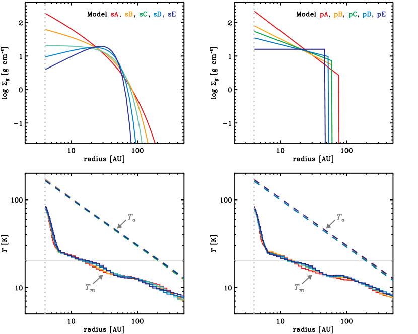
Figure 3: (top) Best-fit gas surface densities (where $\Sigma_{g}=\Sigma_{d}/\zeta$). Similarity solution models are shown on the left and power-law + sharp edge models are shown on the right. (bottom) Temperature profiles at the disk midplane ($T_{m}$) are shown as solid curves, and were determined from RADMC radiative transfer calculations. The parametric atmosphere temperatures ($T_{a}$; at a height $z_{q}$, see §4.2) are overlaid as dashed curves. All models have a gap at $r=4$ AU, marked with a dotted gray line. The CO freezeout temperature, $T_{\rm frz}=20$ K, is marked as a horizontal gray line. The temperature profiles shown here are similar for all models: the midplane values do not change much because the total irradiated dust mass is roughly the same in each case, and the atmosphere temperatures are determined from the same CO emission data. However, each model does have slight variation in the vertical temperature profile, which is not displayed here for the sake of clarity.

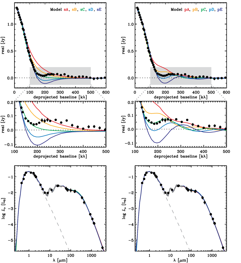
Figure 4: A comparison of the model structures in Table 2 with observations of the dust continuum emission from the TW Hya disk, including the 870 $\mu$m visibility profile (top, with a zoomed-in view of the emission on longer baselines in the middle) and SED (bottom). The similarity solution surface density models (Eq. 2) are shown on the left, and the power-law models with sharp outer edges (Eq. 3) are shown on the right. The model SEDs are essentially indistinguishable, but there are clear differences in the 870 $\mu$m radial emission profiles. The overall best match to the continuum emission is Model pC, which has a density gradient $p=0.75$ and a sharp outer edge at $r_{0}=60$ AU (for the similarity solution models, the best match is Model sC).

4.3 Modeling Results

The best-fit parameters for a range of representative surface density gradients of each model type are compiled in Table 2. For clear notation, each model is labeled with a letter designation corresponding to its $\gamma$ or $p$ value, preceded by a lower-case ‘s’ for the similarity solution models (based on Eq. 2) or ‘p’ for the power-law models (based on Eq. 3). The surface densities, characteristic dust heights, and gas atmosphere temperatures are listed for a radius of 10 AU, where the two surface density model types have comparable behavior. The four parameters describing the dust densities, {$\Sigma_{d}(10)$, $\gamma$ or $p$, $r_{c}$ or $r_{0}$, $z_{d}(10)$}, were determined from joint fits to the SED and 870 $\mu$m continuum visibilities. With those parameters fixed, the gas temperature parameters {$T_{a}(10)$, $q$} were estimated from the CO $J$=3$-$2 visibilities only. The individual $\chi^{2}$ values for the SED, continuum visibilities, and CO visibilities are listed in Cols. (8)-(10). There are 77 independent datapoints in the SED (including 45 equally-spaced points across the Spitzer IRS spectrum), 166,796 continuum visibilities, and 83,740 CO visibilities in each of 15 spectral channels (a total of 1,256,100). The $\chi^{2}$ values were calculated with weights that incorporate the quadrature sum of the formal uncertainties and absolute calibration uncertainties on each datapoint (e.g., a 10% systematic uncertainty on the amplitudes). Figure 3 shows the radial structures for each of the disk models in Table 2, including their surface densities (top) and temperature profiles (bottom).

Figure 4 directly compares the 870 $\mu$m visibilities and SEDs for these model structures with the observations. All of the model structures provide excellent fits to the broadband SED and Spitzer IRS spectrum. Individual SED model behaviors are indistinguishable, aside from small deviations near the far-infrared turnover where the measurement uncertainties are largest. However, the different structures and model types exhibit distinctive signatures in their resolved 870 $\mu$m emission profiles. The similarity solution models with positive density gradients ($\gamma>0$; Models sA and sB) substantially over-predict the emission on $\sim$100-200 k$\lambda$ scales, while those with negative gradients ($\gamma<0$; Models sD and sE) have visibility nulls at $\sim$150 k$\lambda$ that are clearly not commensurate with the data. With an intermediate $\gamma=0$, Model sC provides the best match to the continuum data for this model type. However, it and all other similarity solution models fail to reproduce the visibility oscillations beyond 200 k$\lambda$. This “ringing” is a classic sign of a sharp edge in the radial emission profile, which is naturally produced with the power-law models described by Eq. (3). For those structures, steep density gradients ($p=1.0$-1.5, Models pA and pB) produce too much emission on 100-200 k$\lambda$ baselines and shallow gradients ($p=0.0$-0.5, Models pD and pE) generate visibility nulls that are not observed. However, an intermediate case with $p=0.75$ (Model pC) is an excellent match to the data, with only a small (albeit significant) departure on 280-380 k$\lambda$ scales. That mismatch is likely related to the shape of the outer edge, although we have not pursued that speculation further. Of all the dust structures explored here, Model pC is clearly favored.

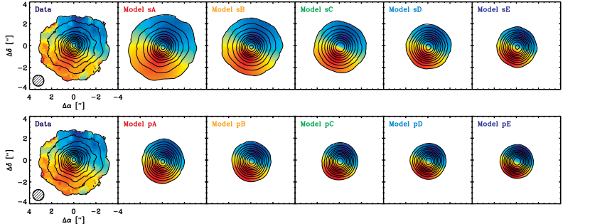
Figure 5: Moment maps of the CO $J$=3$-$2 emission from the TW Hya disk and the various disk structure models compiled in Table 2. The leftmost panels show the SMA observations. The top panels make a direct comparison with the similarity solution models, and the bottom panels do the same for the power-law models with sharp edges. In all plots, contours mark the velocity-integrated CO intensities (0^th moment) at 0.4 Jy km s^-1 ($\sim$3 $\sigma$) intervals and the color scale corresponds to the intensity-weighted line velocities (1^st moment). Only Model sA provides a good match to the observed CO emission; all others predict gas distributions that are too small relative to observations.

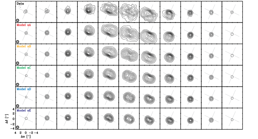
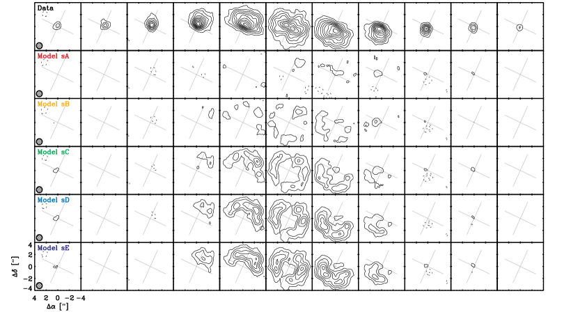
Figure 6: A direct comparison of the observed CO $J$=3$-$2 channel maps with synthetic data from the similarity solution models in Table 2. The top block of panels show the model spectral visibilities synthesized in the same way as the data, and the bottom block displays the imaged residual visibilities. All maps have the same contour intervals as in Figure 1$d$. The viewing geometry of the TW Hya disk is marked with a gray cross in each channel map.

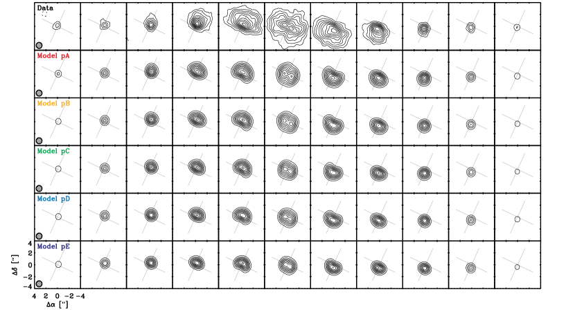
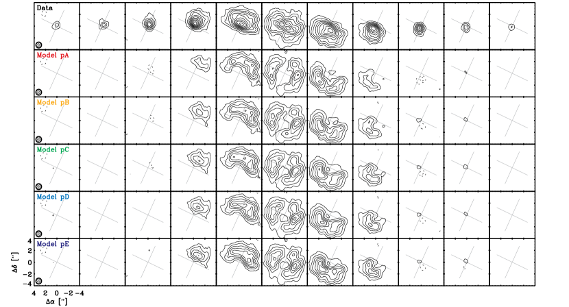
Figure 7: Same as Figure 6, but for the power-law models with sharp outer edges.

A consistent feature of all the dust-based model structures is their compactness. The similarity solution models require characteristic radii of $r_{c}=35$-45 AU and the power-law models call for sharp outer edges at $r_{0}=51$-77 AU. That compact dust distribution was noted in §3, where we pointed out that all of the 870 $\mu$m dust continuum emission is concentrated inside a radius of roughly 1″ ($\sim$60 AU; see Figure 1$a$). Given the much larger radial extent of the CO $J$=3$-$2 emission – out to radii of at least 4″ (215 AU; see Figure 1$d$) – the best-fit models face major problems reconciling the CO and dust observations. The moment maps in Figure 5 confirm this tension between the dust-based structure models and CO data, highlighting a clear CO-dust size discrepancy in nearly all cases. More direct comparisons of the CO channel maps with each model structure can be made in Figures 6 and 7, which show both the models (top panels) and the imaged residual visibilities (bottom panels) synthesized in the same way as the data. Thanks to the freedom afforded by the parametric treatment of the gas temperatures, all models successfully reproduce the central CO emission core that is generated in the line wings. However, only Model sA has a sufficient amount of mass at large disk radii to account for the observations near the systemic velocity. Unfortunately, Model sA provides a poor match to the resolved 870 $\mu$m continuum emission profile.

Before investigating potential physical explanations for the apparent CO-dust size discrepancy, it is important to evaluate the possibility that this is an artifact of some assumption in the modeling (aside from the underlying parametric models themselves; see §5). Admittedly, we adopted a relaxed approach for treating the relative vertical distributions of gas and dust in these models. Only two basic requirements were enforced for consistency: the gas and dust are in thermal equilibrium at the disk midplane, and the gas is distributed vertically according to hydrostatic pressure equilibrium. There are more sophisticated treatments of the gas in disk atmospheres that accurately account for the effects that X-ray heating, chemical differentiation, and gas-dust temperature departures have on the vertical structure of the disk (e.g., van Zadelhoff et al., 2001; Jonkheid et al., 2004; Kamp & Dullemond, 2004; Kamp et al., 2010; Woitke et al., 2009, 2010; Aresu et al., 2011). A nearby disk like TW Hya would benefit from a more detailed analysis with such models, particularly using multiple resolved molecular lines (see Thi et al., 2010, for a start). With a more physically motivated treatment of the vertical structure, we might infer a quantitatively different set of atmosphere properties that would affect the normalization and shape of the CO emission profile (currently controlled by {$T_{1}$, $q$} and other fixed parameters; see §4.2). However, the added complexity of those models would not change the fact that a compact density distribution is required to explain the dust emission. And since we assumed that the CO gas traces the dust in the radial direction, the size discrepancy would remain: these dust-based density profiles do not have enough material to be able to excite CO emission lines at large disk radii (see Figure 3).

To summarize, the fundamental conclusion from the radiative transfer modeling analysis of the SMA data is that the spatial distributions of the CO and millimeter-sized dust in the TW Hya disk are different: the dust is systematically inferred to be more compact than the CO gas.

5 Discussion

We used the SMA to observe the 870 $\mu$m continuum and CO $J$=3$-$2 line emission from the disk around the nearby young star TW Hya. These data represent the most sensitive high spatial resolution (down to scales of 16 AU) probes of the millimeter-wave dust and molecular gas content in any circumstellar disk to date. Along with the SED, these observations were used in concert with continuum and line radiative transfer calculations in an effort to extract the disk density structure. We were unable to identify a consistent model structure that simultaneously accounts for the observed radial distributions of CO and dust. Assuming a radially constant grain size distribution and (vertically integrated) gas-to-dust mass ratio, the millimeter-sized dust structure is significantly more compact than the CO. The resolved continuum emission profile demonstrates that the radial distribution of the millimeter-sized solids in the TW Hya disk has a relatively sharp outer edge near 60 AU, which is considerably smaller than the observed extent of the CO emission (out to at least 215 AU).

The TW Hya disk structure has been studied extensively with millimeter-wave observations at lower angular resolution. In a series of investigations focused almost exclusively on spectral line emission, Qi et al. (2004, 2006, 2008) and Hughes et al. (2011) relied on a slightly modified version of the physical structure model that was developed by Calvet et al. (2002) to match the TW Hya SED. While that model has been used quite successfully to explain the molecular gas structure, there has always been some tension between observations and its predicted millimeter/radio continuum emission profile (see Qi et al., 2004; Wilner et al., 2003, 2005). Given the modest quality of the previous continuum data and the fact that this structure model was not designed (or fitted) with access to resolved observations of any kind, the disagreement was understandably dismissed. As might be expected from its assumption of a “steady” accretion disk structure (i.e., with a large, positive surface density gradient), the Calvet et al. (2002) model exhibits the same type of behavior as Models sA/B or pA/B: it agrees with the data on large scales ($<$100 k$\lambda$), but significantly over-predicts the amount of emission on smaller scales. The same is true for the parametric similarity solution models (where $\gamma\approx 1$) explored by Hughes et al. (2008, 2011), and would certainly apply to the analogous models developed by Thi et al. (2010) and Gorti et al. (2011). All of this previous modeling work admirably reproduces the extended molecular line emission that is observed, and in many cases the SED and millimeter-wave continuum emission on large angular scales as well. It is only with the sensitive, high angular resolution data presented here that we recognize a problem: the radial distribution of the millimeter-sized dust grains is much more compact than for the CO.

Unlike the thermal radiation at millimeter wavelengths, the optical and near-infrared light that scatters off small ($\leq$1 $\mu$m) grains in the TW Hya disk surface is detected out to large distances from the central star – at least $\sim$4″, comparable to what is inferred from CO spectral images (Krist et al., 2000; Trilling et al., 2001; Weinberger et al., 2002; Apai et al., 2004; Roberge et al., 2005). So some dust traces the molecular gas, even if it is only a limited mass of small grains up in the disk atmosphere. However, these exquisitely detailed scattered light images exhibit subtle structural complexities. Krist et al. (2000) identified four distinct radial zones in the optical scattered light disk, with a prominent steepening of the brightness distribution just outside a radius of 50 AU ($\sim$1″; their Zone 1/2 boundary). Similar infrared behavior is noted in the studies by Weinberger et al. (2002) and Apai et al. (2004), which both suggested a break in the emission profile in the 50-80 AU ($\sim$1.0-1.5″) range. Those results were confirmed in a comprehensive analysis of new data by Roberge et al. (2005), who also called attention to a color change at a similar radius as well as an azimuthal asymmetry out to a slightly larger distance from the star ($\sim$135 AU). The physical origin of these scattered light features has been a mystery, although speculation centered around variations in the dust height (shadowing) and gradients in the dust scattering properties (either mineralogical or size-related). But in light of our discovery of an abrupt drop in the millimeter-wave continuum emission at the same location as these features, it is only natural to suspect that a more fundamental change occurs in the physical structure of the TW Hya dust disk near 60 AU.

Perhaps the most straightforward explanation of the apparent CO-dust size discrepancy inferred from the SMA data is that we have used an incomplete description of the disk structure. As an example, consider a modification of either model type that incorporates an abrupt decrease in the surface densities (or millimeter-wave dust opacities) – not the dust-to-gas ratio – outside $r\approx 60$ AU. If that drop in $\Sigma$ (or $\kappa_{\rm mm}$) was not too large (perhaps a factor of $\sim$100), there would still be enough disk material to produce bright emission from the optically thick CO lines and scattered light while also accounting for the sharp edge feature noted in the optically thin 870 $\mu$m emission profile. That “substructure” in the outer dust disk might actually enhance the local gas-phase CO abundance, as ultraviolet radiation can penetrate deeper into the disk interior and photodesorb CO from the (small) reservoir of cold dust grains that remains at large radii (e.g., Hersant et al., 2009).

Nevertheless, a physical origin for such a dramatic drop in the dust densities and/or the millimeter-wave dust opacities is not obvious. One possibility is that the disk has been perturbed by a long-period (as yet unseen) companion. If a faint object is embedded in the disk near the apparent edge of the 870 $\mu$m emission distribution, it might open a gap that splits the disk into two distinct reservoirs and generate the warp asymmetry suggested by Roberge et al. (2005). But, a narrow gap alone would not account for the SMA continuum observations. The millimeter-wave luminosity exterior to the gap would still need to be decreased, perhaps because the particles at those larger radii were preferentially unable to grow to millimeter sizes. Weinberger et al. (2002) quote deep limits on $H$-band point sources in the TW Hya disk that suggest there are no companions more massive than $\sim$6 M_Jup near 60 AU, according to the Baraffe et al. (2003) models (the corresponding mass limit is higher for the models of Marley et al., 2007). Certainly this kind of truncation or other forms of substructure could be invoked to explain the sharp radial edge in the SMA dust observations. But rather than engage in further speculation on the details, it should suffice to point out that the potential for substructure or other anomalies in the TW Hya disk can be tested with a substantial increase in resolution and sensitivity. Moreover, spectral imaging of optically thinner gas tracers (e.g., the CO isotopologues) would make for an ideal test of the origins of the apparent CO-dust size discrepancy. Fortunately, such observations will shortly be available as the Atacama Large Millimeter Array (ALMA) begins routine science operations.

There is a compelling alternative explanation that has a more concrete physical motivation. In any protoplanetary disk, the thermal pressure of the gas is thought to cause it to orbit the star at slightly sub-Keplerian rates, generating a small velocity difference relative to the particles embedded in it (Weidenschilling, 1977). Depending on their size, particles can experience a head-wind from this gas drag that decays their orbits and sends them spiraling in toward the central star. This radial drift of particles modifies the radial dust-to-gas mass ratio profile and introduces a pronounced spatial gradient in the particle size distribution – in essence, it causes $\zeta$ and $\kappa_{\rm mm}$ to decrease with radius (Brauer et al., 2007, 2008; Birnstiel et al., 2009). In the outer disk, the drift rates are expected to be largest for millimeter-sized particles (e.g., Takeuchi & Lin, 2002). Since thermal emission peaks at a wavelength comparable to the particle size, the drift process should then naturally produce a millimeter-wave emission profile that is considerably more compact than would be inferred from tracers of the gas (Takeuchi & Lin, 2005). Moreover, the dust particles that reflect light in the disk atmosphere are small enough to be dynamically coupled to the gas – therefore, scattered light images should be extended like the probes of the gas phase.

From a qualitative perspective, our analysis of the CO and dust structures in the TW Hya disk are certainly consistent with a scenario where growth and radial drift have had an observable impact. However, it is unclear if realistic models of the growth and migration of solids in a disk like this can quantitatively account for the details. One particular challenge worth highlighting is related to timescales. The Takeuchi & Lin (2005) models suggest that millimeter-wave dust emission should be strongly attenuated on a timescale of $\sim$1 Myr without constant replenishment (presumably from growth and/or fragmentation). Given the advanced age of TW Hya ($\sim$8-20 Myr), this model would require either that replenishment shuts off after several Myr or that drift is inefficient at early times before becoming more important later in the disk evolution process. If this is indeed the mechanism responsible for our results, additional observations of disks at a range of ages could be used to help calibrate models of the long-term evolution of drift rates. One potential way to test this hypothesis relies on the particle size dependence of the radial drift rates. The theory implies that larger particles will end up with more centrally concentrated density distributions. At long and optically thin wavelengths, we expect that the size of the continuum emission region should be anti-correlated with wavelength – longer wavelengths imply more compact emission. In principle, this could be tested in the near future by combining high resolution ALMA and Expanded Very Large Array (EVLA) observations of the TW Hya dust disk that span the millimeter/radio spectrum.

In many ways, TW Hya and its disk are unique and may not be representative of the bulk population of pre-main sequence stars and their circumstellar material. Nevertheless, it is worth considering the broader implications of our findings for this specific example – they may prove to be more generally applicable. It is possible that the CO-dust size discrepancy found here is present in most other millimeter-wave disk observations, but it would likely be difficult to identify with current sensitivity and resolution limitations. If that feature is common and its underlying cause is a drop in the dust-to-gas ratio in the outer disk, there would be serious consequences for disk mass estimates based on dust continuum measurements. There could be large and hidden mass reservoirs of molecular gas in the outer reaches of protoplanetary disks, implying that disk masses might be substantially under-estimated. If true, gas densities at large disk radii may be higher than typically assumed, with profound implications for facilitating giant planet formation by gravitational instability (e.g., Boley, 2009; Kratter et al., 2010; Boss, 2011). However, if radial drift is the key process responsible for the apparent CO-dust size discrepancy, it is also possible that any “primordial” dust-to-gas ratio integrated over the entire disk is preserved. This would be the case if the millimeter-sized dust originally present at large radii had its inward migration halted before it was accreted onto the central star. In that scenario, the total disk mass estimates from millimeter-wave luminosities would still be relatively accurate (assuming a proper model for the dust opacities that considers the simultaneous particle size evolution is available), although the densities in the outer disk would remain uncertain without measurements of optically thin gas emission lines.

Independent of the apparent CO-dust size discrepancy, our finding that the millimeter-wave continuum emission from the TW Hya disk is so sharply truncated comes as a surprise. Modern interferometric datasets generally do not have sufficient sensitivity to differentiate between dust density models with sharp edges or smooth tapers (e.g., see Isella et al., 2010; Guilloteau et al., 2011). Given that ambiguity, it is possible that the edge feature we have identified in the 870 $\mu$m emission profile of the TW Hya disk could be relatively common. Moreover, it is tempting to associate this $r\approx 60$ AU edge in the distribution of larger solid particles in the TW Hya disk with the similarly abrupt truncation of the classical Kuiper Belt at $r\approx 40$-50 AU in our solar system (Trujillo et al., 2001; Gladman et al., 2001). If this behavior ends up being a generic feature in protoplanetary disks, it may signify an important diagnostic of the radial migration of disk solids and provide new insights into the structural origins and evolution of the outer solar system (e.g., see Kenyon & Luu, 1999; Levison & Morbidelli, 2003).

Further speculation on the generality of the features identified in the TW Hya disk is unnecessary. With the recent start of ALMA science operations, the quality of the data presented here will be matched (and exceeded) routinely for large samples, and the basic trends of disk properties like those probed here will be clarified. If the TW Hya disk is not anomalous, it is clear that the general methods used to interpret observations of dust in disks will need to be modified to focus less on their bulk density structures and more on the dynamical evolution of their solid contents.

6 Summary

We have presented sensitive, high resolution ($0\farcs 3=16$ AU) SMA observations of the 870 $\mu$m continuum and CO $J$=3$-$2 line emission from the disk around the nearby young star TW Hya. Based on two different parametric formulations for the disk densities, we used radiative transfer calculations to compare the predicted radial structures of the dust and CO gas in the TW Hya disk with these SMA observations and ancillary measurements of the spectral energy distribution. The key conclusions from this modeling analysis of these high-quality data include:

1. Under the assumption that the dust-to-gas surface density ratio is constant with radius, we were not able to find any model structure that can simultaneously reproduce the resolved brightness profiles of the 870 $\mu$m continuum and CO line emission. We have identified a clear CO-dust size discrepancy that is present regardless of whether the assumed surface density profile has a sharp outer edge or a smooth (exponential) taper at large radii.

2. The radial distribution of millimeter-sized dust grains in the TW Hya disk is substantially more compact than its CO gas reservoir. The 870 $\mu$m dust emission has a sharp outer edge near 60 AU, while the CO emission (and optical/infrared scattered light from small grains that are dynamically coupled to the gas) extends to a radius of at least 215 AU.

3. The observationally inferred CO-dust size discrepancy could potentially be explained with a more complex dust density profile that exhibits a sudden decrease by a large factor near a radius of 60 AU. That “break” in the density profile might be consistent with a tidal perturbation by a long-period (unseen) companion, although the dust at larger radii would then also have to be preferentially depleted of millimeter-sized grains.

4. Alternatively, the observations might have uncovered some preliminary evidence for a key evolutionary mechanism related to the planet formation process: the growth and inward migration of disk solids. The radial drift of millimeter-sized particles is expected to naturally concentrate long-wavelength thermal emission near the star relative to tracers of the molecular gas reservoir. However, a more detailed exploration of disk evolution models is needed to verify if the observations of the TW Hya disk are quantitatively consistent with this scenario.

References

- Aikawa & Nomura (2006) Aikawa, Y., & Nomura, H. 2006, ApJ, 642, 1152
- Akeson et al. (2011) Akeson, R. L., et al. 2011, ApJ, 728, 96
- Andrews et al. (2008) Andrews, S. M., Hughes, A. M., Wilner, D. J., & Qi, C. 2008, ApJ, 678, L133
- Andrews et al. (2009) Andrews, S. M., Wilner, D. J., Hughes, A. M., Qi, C., & Dullemond, C. P. 2009, ApJ, 700, 1502
- Andrews et al. (2010a) Andrews, S. M., Czekala, I., Wilner, D. J., Espaillat, C., Dullemond, C. P., & Hughes, A. M. 2010, ApJ, 710, 462 (2010a)
- Andrews et al. (2010b) Andrews, S. M., Wilner, D. J., Hughes, A. M., Qi, C., & Dullemond, C. P. 2010, ApJ, 723, 1241 (2010b)
- Andrews et al. (2011) Andrews, S. M., et al. 2011, ApJ, 732, 42
- Apai et al. (2004) Apai, D., et al. 2004, A&A, 415, 671
- Aresu et al. (2011) Aresu, G., Kamp, I., Meijerink, R., Woitke, P., Thi, W.-F., & Spaans, M. 2011, A&A, 526, 163
- Baraffe et al. (2003) Baraffe, I., Chabrier, G., Barman, T. S., Allard, F., & Hauschildt, P. H. 2003, A&A, 402, 701
- Birnstiel et al. (2009) Birnstiel, T., Dullemond, C. P., & Brauer, F. 2009, A&A, 503, L5
- Boley (2009) Boley, A. C. 2009, ApJ, 695, L53
- Boss (2011) Boss, A. P. 2011, ApJ, 731, 74
- Brauer et al. (2007) Brauer, F., Dullemond, C. P., Henning, T., Klahr, H., & Natta, A. 2007, A&A, 469, 1169
- Brauer et al. (2008) Brauer, F., Dullemond, C. P., & Henning, T. 2008, A&A, 859, 480
- Brinch & Hogerheijde (2010) Brinch, C., & Hogerheijde, M. R. 2010, A&A, 523, 25
- Calvet et al. (2002) Calvet, N., D’Alessio, P., Hartmann, L., Wilner, D. J., Walsh, A., & Sitko, M. 2002, 568, 1008
- Cutri et al. (2003) Cutri, R. M., et al. 2003, 2MASS All-Sky Point Source Catalog (Pasadena: IPAC)
- D’Alessio et al. (1999) D’Alessio, P., Calvet, N., Hartmann, L., Lizano, S., & Cantó, J. 1999, ApJ, 527, 893
- D’Alessio et al. (2001) D’Alessio, P., Calvet, N., & Hartmann, L. 2001, ApJ, 553, 321
- Dartois et al. (2003) Dartois, E., Dutrey, A., & Guilloteau, S. 2003, A&A, 399, 773
- Di Francesco et al. (2008) Di Francesco, J., Johnstone, D., Kirk, H., MacKenzie, T., & Ledwosinska, E. 2008, ApJS, 175, 277
- Dullemond & Dominik (2004a) Dullemond, C. P., & Dominik, C. 2004, A&A, 417, 159 (2004a)
- Dutrey et al. (2007) Dutrey, A., Guilloteau, S., & Ho, P. 2007, in Protostars & Planets V, eds. B. Reipurth, D. Jewitt, & K. Keil (Univ. Arizona Press: Tucson), 495
- Eisner et al. (2006) Eisner, J. A., Chiang, E. I., & Hillenbrand, L. A. 2006, ApJ, 637, L133
- Gladman et al. (2001) Gladman, B., et al. 2001, AJ, 122, 1051
- Gorti et al. (2011) Gorti, U., Hollenbach, D., Najita, J., & Pascucci, I. 2011, ApJ, 735, 90
- Guilloteau et al. (2011) Guilloteau, S., Dutrey, A., Piétu, V., & Boehler, Y. 2011, A&A, 529, 105
- Hartmann et al. (2005) Hartmann, L., et al. 2005, ApJ, 629, 881
- Hersant et al. (2009) Hersant, F., Wakelam, V., Dutrey, A., Guilloteau, S., & Herbst, E. 2009, A&A, 493, L49
- Ho et al. (2004) Ho, P. T. P., Moran, J. M., & Lo, K. Y. 2004, ApJ, 616, L1
- Hughes et al. (2007) Hughes, A. M., Wilner, D. J., Calvet, N., D’Alessio, P., Claussen, M. J., & Hogerheijde, M. R. 2007, ApJ, 664, 536
- Hughes et al. (2008) Hughes, A. M., Wilner, D. J., Qi, C., & Hogerheijde, M. R. 2008, ApJ, 678, 1119
- Hughes et al. (2010) Hughes, A. M., et al. 2010, AJ, 140, 887
- Hughes et al. (2011) Hughes, A. M., Wilner, D. J., Andrews, S. M., Qi, C., & Hogerheijde, M. R. 2010, ApJ, 727, 85
- Isella et al. (2007) Isella, A., Testi, L., Natta, A., Neri, R., Wilner, D., & Qi, C. 2007, A&A, 469, 213
- Isella et al. (2009) Isella, A., Carpenter, J. M., & Sargent, A. I. 2009, ApJ, 701, 260
- Isella et al. (2010) Isella, A., Carpenter, J. M., & Sargent, A. I. 2010, ApJ, 714, 1746
- Jäger et al. (2003) Jäger, C., Dorschner, J., Mutschke, H., Posch, T., & Henning, T. 2003, A&A, 408, 193
- Jonkheid et al. (2004) Jonkheid, B., Faas, F. G. A., van Zadelhoff, G.-J., & van Dishoeck, E. F. 2004, A&A, 428, 511
- Kamp & Dullemond (2004) Kamp, I., & Dullemond, C. P. 2004, ApJ, 615, 991
- Kamp et al. (2010) Kamp, I., Tilling, I., Woitke, P., Thi, W.-F., & Hogerheijde, M. R. 2010, A&A, 510, 18
- Kastner et al. (1997) Kastner, J. H., Zuckerman, B., Weintraub, D. A., & Forveille, T. 1997, Science, 277, 67
- Kenyon & Luu (1999) Kenyon, S. J., & Luu, J. X. 1999, ApJ, 526, 465
- Kratter et al. (2010) Kratter, K. M., Murray-Clay, R. A., & Youdin, A. N. 2010, ApJ, 710, 1375
- Krist et al. (2000) Krist, J. E., Stapelfeldt, K. R., Ménard, F., Padgett, D. L., & Burrows, C. J. 2000, ApJ, 538, 793
- Lejeune et al. (1997) Lejeune, T., Cuisinier, F., & Buser, R. 1997, A&AS, 125, 229
- Levison & Morbidelli (2003) Levison, H. F., & Morbidelli, A. 2003, Nature, 426, 419
- Low et al. (2005) Low, F. J., et al. 2005, ApJ, 631, 1170
- Lynden-Bell & Pringle (1974) Lynden-Bell, D., & Pringle, J. E. 1974, MNRAS, 168, 603
- Marley et al. (2007) Marley, M. S., Fortney, J. J., Hubickyj, O., Bodenheimer, P., & Lissauer, J. J. 2007, ApJ, 655, 541
- Mekkaden (1998) Mekkaden, M. V. 1998, A&A, 340, 135
- Panić et al. (2009) Panić, O., Hogerheijde, M. R., Wilner, D., & Qi, C. 2009, A&A, 501, 269
- Perryman et al. (1997) Perryman, M. A. C., et al. 1997, A&A, 323, L49
- Piétu et al. (2005) Piétu, V., Guilloteau, S., & Dutrey, A. 2005, A&A, 443, 945
- Pinte et al. (2008) Pinte, C., et al. 2008, A&A, 489, 633
- Pollack et al. (1994) Pollack, J. B., Hollenbach, D., Beckwith, S., Simonelli, D. P., Roush, T., & Fong, W. 1994, ApJ, 421, 615
- Qi et al. (2004) Qi, C., et al. 2004, ApJ, 616, L11
- Qi et al. (2006) Qi, C., et al. 2006, ApJ, 636, L157
- Qi et al. (2008) Qi, C., Wilner, D. J., Aikawa, Y., Blake, G. A., & Hogerheijde, M. R. 2008, ApJ, 681, 1396
- Qi et al. (2011) Qi, C., D’Alessio, P., Öberg, K. I., Wilner, D. J., Hughes, A. M., Andrews, S. M., & Ayala, S. 2011, ApJ, 740, 84
- Ratzka et al. (2007) Ratzka, T., Leinert, C., Henning, T., Bouwman, J., Dullemond, C. P., & Jaffe, W. 2007, A&A, 471, 173
- Roberge et al. (2005) Roberge, A., Weinberger, A. J., & Malumuth, E. M. 2005, ApJ, 622, 1171
- Rucinski & Krautter (1983) Rucinski, S. M., & Krautter, J. 1983, A&A, 121, 217
- Takeuchi & Lin (2002) Takeuchi, T., & Lin, D. N. C. 2002, ApJ, 581, 1344
- Takeuchi & Lin (2005) Takeuchi, T., & Lin, D. N. C. 2005, ApJ, 623, 482
- Thi et al. (2010) Thi, W.-F., et al. 2010, A&A, 518, L125
- Trilling et al. (2001) Trilling, D. E., Koerner, D. W., Barnes, J. W., Ftaclas, C., & Brown, R. H. 2001, ApJ, 522, L151
- Trujillo et al. (2001) Trujillo, C. A., Jewitt, D. C., & Luu, J. X. 2001, AJ, 122, 457
- Uchida et al. (2004) Uchida, K. I., et al. 2004, ApJS, 154, 439
- Vacca & Sandell (2011) Vacca, W. D., & Sandell, G. 2011, ApJ, 732, 8
- van Leeuwen (2007) van Leeuwen, F. 2007, A&A, 474, 653
- van Zadelhoff et al. (2001) van Zadelhoff, G.-J., van Dishoeck, E. F., Thi, W.-F., & Blake, G. A. 2001, A&A, 377, 566
- Weaver & Jones (1992) Weaver, W. B., & Jones, G. 1992, ApJS, 78, 239
- Webb et al. (1999) Webb, R. A., et al. 1999, ApJ, 512, L63
- Weidenschilling (1977) Weidenschilling, S. J., MNRAS, 180, 57
- Weinberger et al. (2002) Weinberger, A. J., et al. 2002, ApJ, 566, 409
- Weintraub et al. (1989) Weintraub, D. A., Sandell, G., & Duncan, W. D. 1989, ApJ, 340, L69
- Weintraub et al. (2000) Weintraub, D. A., Saumon, D., Kastner, J. H., & Forveille, T. 2000, ApJ, 530, 867
- Wichmann et al. (1998) Wichmann, R., Bastian, U., Krautter, J., Jankovics, I., & Rucinski, S. M. 1998, MNRAS, 301, L39
- Williams & Cieza (2011) Williams, J. P., & Cieza, L. A. 2011, ARA&A, 49, 67
- Wilner et al. (2000) Wilner, D. J., Ho, P. T. P., Kastner, J. H., & Rodríguez, L. F. 2000, ApJ, 534, L101
- Wilner et al. (2003) Wilner, D. J., Bourke, T. L., Wright, C. M., Jorgensen, J. K., van Dishoeck, E. F., & Wong, T. 2003, ApJ, 596, 597
- Wilner et al. (2005) Wilner, D. J., D’Alessio, P., Calvet, N., Claussen, M. J., & Hartmann, L. 2005, ApJ, 626, L109
- Woitke et al. (2009) Woitke, P., Kamp, I., & Thi, W.-F. 2009, A&A, 501, 383
- Woitke et al. (2010) Woitke, P., et al. 2010, MNRAS, 405, L26
- Yang et al. (2005) Yang, H., Johns-Krull, C. M., & Valenti, J. A. 2005, ApJ, 635, 466