Mean Width of a Regular Simplex

Abstract

The mean width is a measure on $n$-dimensional convex bodies. An integral formula for the mean width of a regular $n$-simplex appeared in the electrical engineering literature in 1997. As a consequence, expressions for the expected range of a sample of $n+1$ normally distributed variables, for $n\leq 6$, carry over to widths of regular $n$-simplices. As another consequence, precise asymptotics for the mean width become available as $n\rightarrow\infty$.

Let $C$ be a convex body in $\mathbb{R}^{n}$. A width is the distance between a pair of parallel $C$-supporting planes (linear varieties of dimension $n-1$). Every unit vector $u\in\mathbb{R}^{n}$ determines a unique such pair of planes orthogonal to $u$ and hence a width $w(u)$. Let $u$ be uniformly distributed on the unit sphere $S^{n-1}\subset$ $\mathbb{R}^{n}$. Then $w$ is a random variable and

$$\mathbb{E}\left(w_{3}\right)=\frac{3}{2\pi}\arccos\left(-\frac{1}{3}\right)$$

for $C=$ the regular $3$-simplex (tetrahedron) in $\mathbb{R}^{3}$ with edges of unit length and

$$\mathbb{E}\left(w_{4}\right)=\frac{10}{3\pi^{2}}\left[3\arccos\left(-\frac{1}{3}\right)-\pi\right]$$

for $C=$ the regular $4$-simplex in $\mathbb{R}^{4}$ with edges of unit length [1, 2].  Our contribution is to extend the preceding mean width results to regular $n$-simplices in $\mathbb{R}^{n}$ for $n\leq 6$. We similarly extend the following mean square width result:

$$\mathbb{E}\left(w_{3}^{2}\right)=\frac{1}{3}\left(1+\frac{3+\sqrt{3}}{\pi}\right)$$

which, as far as is known, first appeared in [3].

The key observation underlying our work is due to Sun [4], which in turn draws upon material in [5, 6].  It does not seem to have been acknowledged in the mathematics literature.  After most of this paper was written, we found [7], which assigns priority to to Hadwiger [8] and to Ruben [9] for closely related ideas.

1 Order Statistics

Let $X_{1},$ $X_{2},$ $...,$ $X_{n}$ denote a random sample from a Normal $(0,1)$ distribution, that is, with density function $f$ and cumulative distribution $F$:

$$\begin{array}[c]{ccc}f(x)=\dfrac{1}{\sqrt{2\pi}}\exp\left(-\dfrac{x^{2}}{2}\right),&&F(x)={\displaystyle\int\limits_{-\infty}^{x}}f(\xi)\,d\xi=\dfrac{1}{2}\operatorname*{erf}\left(\dfrac{x}{\sqrt{2}}\right)+\dfrac{1}{2}.\end{array}$$

The first two moments of the range

$$r_{n}=\max\{X_{1},X_{2},...,X_{n}\}-\min\{X_{1},X_{2},...,X_{n}\}$$

are given by [10, 11]

$$\mu_{n}=\mathbb{E}(r_{n})={\displaystyle\int\limits_{-\infty}^{\infty}}\left\{1-F(x)^{n}-[1-F(x)]^{n}\right\}dx,$$

$$\nu_{n}=\mathbb{E}(r_{n}^{2})=2{\displaystyle\int\limits_{-\infty}^{\infty}}{\displaystyle\int\limits_{-\infty}^{y}}\left\{1-F(y)^{n}-[1-F(x)]^{n}+[F(y)-F(x)]^{n}\right\}dx\,dy.$$

For small $n$, exact expressions are possible [12, 13, 14]:

$$\begin{array}[c]{lll}\mu_{2}=\frac{2}{\sqrt{\pi}}=1.128...,&&\begin{array}[c]{c}\nu_{2}=2,\end{array}\\ \mu_{3}=\frac{3}{\sqrt{\pi}}=1.692...,&&\begin{array}[c]{c}\nu_{3}=2\left(1+\frac{3\sqrt{3}}{2\pi}\right)=3.653...,\end{array}\\ \mu_{4}=\frac{6}{\sqrt{\pi}}\left(1-2S_{2}\right)=2.058...,&&\begin{array}[c]{c}\nu_{4}=2\left(1+\frac{3+\sqrt{3}}{\pi}\right)=5.012...,\end{array}\\ \mu_{5}=\frac{10}{\sqrt{\pi}}\left(1-3S_{2}\right)=2.325...,&&\begin{array}[c]{c}\nu_{5}=2\left(1+\frac{5\sqrt{3}}{2\pi}+\frac{30}{\pi}S_{1/2}-\frac{5\sqrt{3}}{\pi}S_{3}\right)=6.156...,\end{array}\\ \mu_{6}=\frac{15}{\sqrt{\pi}}\left(1-4S_{2}+2T_{2}\right)=2.534...,&&\begin{array}[c]{c}\nu_{6}=2\left(1+\frac{5(9+2\sqrt{3})}{2\pi}-\frac{90}{\pi}S_{2}-\frac{15\sqrt{3}}{\pi}S_{3}\right)=7.142...,\end{array}\\ \mu_{7}=\frac{21}{\sqrt{\pi}}\left(1-5S_{2}+5T_{2}\right)=2.704...,&&\begin{array}[c]{l}\nu_{7}=2\left(1+\frac{35\sqrt{3}}{4\pi}+\frac{210}{\pi}S_{1/2}-\frac{105}{\pi}S_{2}-\frac{35\sqrt{3}}{\pi}S_{3}\right.\\ \;\;\;\;\;\;\;\;\;\;\;\;\;\;\;\left.+\frac{35\sqrt{3}}{2\pi}T_{3}+\frac{210}{\pi}U-\frac{420}{\pi}V\right)=8.007...\end{array}\end{array}$$

where

$$S_{k}=\frac{\sqrt{k}}{\pi}{\displaystyle\int\limits_{0}^{\pi/4}}\frac{dx}{\sqrt{k+\sec(x)^{2}}}=\frac{1}{2\pi}\operatorname{arcsec}\left(k+1\right),$$

$$T_{k}=\frac{\sqrt{k}}{\pi^{2}}{\displaystyle\int\limits_{0}^{\pi/4}}\,{\displaystyle\int\limits_{0}^{\pi/4}}\frac{dx\,dy}{\sqrt{k+\sec(x)^{2}+\sec(y)^{2}}}=\frac{1}{2\pi^{2}}{\displaystyle\int\limits_{0}^{\pi\,S_{k}}}\operatorname{arcsec}\left(1+\frac{k(k+1)}{k-\tan(z)^{2}}\right)dz,$$

$$\begin{array}[c]{ccc}U=\dfrac{1}{\pi^{2}}{\displaystyle\int\limits_{0}^{1}}\dfrac{\operatorname{arcsec}\left(2t^{2}+4\right)}{\left(2t^{2}+1\right)\sqrt{2t^{2}+3}}dt,&&V=\dfrac{1}{\pi^{2}}{\displaystyle\int\limits_{0}^{1}}\dfrac{\operatorname{arcsec}\left(t^{2}+5\right)}{\left(t^{2}+2\right)\sqrt{t^{2}+4}}dt.\end{array}$$

The preceding table complements an analogous table in [15] for first and second moments of $\max\{X_{1},X_{2},...,X_{n}\}$. Similar expressions for $\mu_{8}=2.847...$ and $\nu_{8}=8.778...$ remain to be found.

2 Key Observation

Let us rescale length so that the circumradius of the $n$-simplex is $1$. Adjusted width will be denoted by $\widetilde{w}_{n}$. Using optimality properties of the $n$-simplex, Sun [4] deduced a formula for mean half width:

$$\frac{1}{2}\mathbb{E}\left(\widetilde{w}_{n}\right) =\frac{n+1}{2}\sqrt{\frac{(n+1)n}{2\pi}}\frac{\Gamma\left(\frac{n}{2}\right)}{\Gamma\left(\frac{n+1}{2}\right)}{\displaystyle\int\limits_{-\infty}^{\infty}}F\left(\tfrac{x}{\sqrt{2}}\right)^{n-1}f(x)\,dx$$

$$=\frac{(n+1)^{3/2}}{\sqrt{2n}}\frac{\Gamma\left(\frac{n}{2}\right)}{\Gamma\left(\frac{n+1}{2}\right)}{\displaystyle\int\limits_{-\infty}^{\infty}}x\,F(x)^{n}f(x)\,dx$$

(see Corollary 2 on p. 1581 and its proof on p. 1585; his $M$ is the same as our $n+1$).  We recognize the latter integral as $\mu_{n+1}/(2(n+1))$; hence

$$\mathbb{E}\left(\widetilde{w}_{n}\right)=\sqrt{\frac{n+1}{2n}}\frac{\Gamma\left(\frac{n}{2}\right)}{\Gamma\left(\frac{n+1}{2}\right)}\mu_{n+1}$$

and therefore

$$\mathbb{E}\left(w_{n}\right)=\frac{1}{2}\frac{\Gamma\left(\frac{n}{2}\right)}{\Gamma\left(\frac{n+1}{2}\right)}\mu_{n+1}$$

because, in our original scaling, the circumradius is $\sqrt{n/(2(n+1))}$.

No similar integral expression for $\mathbb{E}\left(\widetilde{w}_{n}^{2}\right)$ appears in [4]. We circumvent this difficulty by noticing that the formula [16, 17]

$$\mathbb{E}\left(\sqrt{{\displaystyle\sum\limits_{k=1}^{n}}X_{k}^{2}}\right)=\sqrt{2}\frac{\Gamma\left(\frac{n+1}{2}\right)}{\Gamma\left(\frac{n}{2}\right)}$$

bears some resemblance to the coefficient of $\mu_{n+1}$ in our expression for $\mathbb{E}\left(w_{n}\right)$. The square version

$$\mathbb{E}\left({\displaystyle\sum\limits_{k=1}^{n}}X_{k}^{2}\right)=n$$

is trivial and leads us to conjecture that

$$\mathbb{E}\left(w_{n}^{2}\right)=\frac{1}{2n}\nu_{n+1}$$

by analogy.  Numerical confirmation for $n\leq 6$ is possible via the computer algebra technique described in [3].

In summary, we have mean width results

$$\mathbb{E}\left(w_{2}\right)=\frac{3}{\pi}=0.954929658551372...,$$

$$\mathbb{E}\left(w_{3}\right)=\frac{3}{2}\left(1-2S_{2}\right)=0.912260171954089...,$$

$$\mathbb{E}\left(w_{4}\right)=\frac{20}{3\pi}\left(1-3S_{2}\right)=0.874843256085440...,$$

$$\mathbb{E}\left(w_{5}\right)=\frac{45}{16}\left(1-4S_{2}+2T_{2}\right)=0.842274297659162...,$$

$$\mathbb{E}\left(w_{6}\right)=\frac{56}{5\pi}\left(1-5S_{2}+5T_{2}\right)=0.813743951590337...,$$

and mean square width results

$$\mathbb{E}\left(w_{2}^{2}\right)=\frac{1}{2}\left(1+\frac{3\sqrt{3}}{2\pi}\right)=0.913496671566344...,$$

$$\mathbb{E}\left(w_{3}^{2}\right)=\frac{1}{3}\left(1+\frac{3+\sqrt{3}}{\pi}\right)=0.835419517991054...,$$

$$\mathbb{E}\left(w_{4}^{2}\right) =\frac{1}{4}\left(1+\frac{5\sqrt{3}}{2\pi}+\frac{30}{\pi}S_{1/2}-\frac{5\sqrt{3}}{\pi}S_{3}\right)$$

$$=0.769572883591771...,$$

$$\mathbb{E}\left(w_{5}^{2}\right) =\frac{1}{5}\left(1+\frac{5(9+2\sqrt{3})}{2\pi}-\frac{90}{\pi}S_{2}-\frac{15\sqrt{3}}{\pi}S_{3}\right)$$

$$=0.714241915072694...,$$

$$\mathbb{E}\left(w_{6}^{2}\right) =\frac{1}{6}\left(1+\frac{35\sqrt{3}}{4\pi}+\frac{210}{\pi}S_{1/2}-\frac{105}{\pi}S_{2}-\frac{35\sqrt{3}}{\pi}S_{3}\right.$$

$$\;\;\;\;\;\;\;\;\left.+\frac{35\sqrt{3}}{2\pi}T_{3}+\frac{210}{\pi}U-\frac{420}{\pi}V\right)$$

$$=0.667314714095430....$$

3 Asymptotics

We turn now to the asymptotic distribution of $r_{n}$ as $n\rightarrow\infty$. Define $a_{n}$ to be the positive solution of the equation [12, 18]

$$2\pi\,a_{n}^{2}\exp\left(a_{n}^{2}\right)=n^{2},$$

that is,

$$a_{n}=\sqrt{W\left(\frac{n^{2}}{2\pi}\right)}\sim\sqrt{2\ln(n)}-\frac{1}{2}\frac{\ln(\ln(n))+\ln(4\pi)}{\sqrt{2\ln(n)}}$$

in terms of the Lambert $W$ function [19].  It can be proved that the required density is a convolution [20, 21]:

$$\lim_{n\rightarrow\infty}\frac{d}{dy}\operatorname*{P}\left(\sqrt{2\ln(n)}(r_{n}-2a_{n})<y\right) ={\displaystyle\int\limits_{-\infty}^{\infty}}\exp(-x-e^{-x})\exp(-(y-x)-e^{-(y-x)})dx$$

$$=2\,e^{-y}K_{0}\left(2\,e^{-y/2}\right)$$

where $K_{0}$ is the modified Bessel function of the second kind [22]. A random variable $Y$, distributed as such, satisfies

$$\begin{array}[c]{ccc}\mathbb{E}(Y)=2\gamma,&&\mathbb{E}(Y^{2})=\dfrac{\pi^{2}}{3}+4\gamma^{2}\end{array}$$

where $\gamma$ is the Euler-Mascheroni constant [23].  This implies that

$$\mu_{n}\sim 2\left(a_{n}+\frac{\gamma}{\sqrt{2\ln(n)}}\right)\sim 2\sqrt{2\ln(n)}-\frac{\ln(\ln(n))+\ln(4\pi)-2\gamma}{\sqrt{2\ln(n)}}$$

and hence

$$\mathbb{E}(w_{n}) =\frac{1}{2}\frac{\Gamma\left(\frac{n}{2}\right)}{\Gamma\left(\frac{n+1}{2}\right)}\mu_{n+1}=\frac{1}{2}\frac{\Gamma\left(\frac{n}{2}\right)}{\Gamma\left(\frac{n+1}{2}\right)}\cdot\frac{\mu_{n+1}}{\mu_{n}}\cdot\mu_{n}$$

$$\sim\frac{1}{\sqrt{2n}}\left(1+\frac{1}{4n}\right)\cdot\left(1+\frac{1}{2n\,\ln(n)}\right)\cdot 2\left(a_{n}+\frac{\gamma}{\sqrt{2\ln(n)}}\right)$$

$$\sim 2\sqrt{\frac{\ln(n)}{n}}-\frac{\ln(\ln(n))+\ln(4\pi)-2\gamma}{2\sqrt{n\ln(n)}}.$$

More terms in the asymptotic expansion are possible.

If we rescale length so that the inradius of the $n$-simplex is $1$ and denote adjusted width by $\widehat{w}_{n}$, then

$$\mathbb{E}(\widehat{w}_{n})\sim\sqrt{2}n\cdot 2\sqrt{\frac{\ln(n)}{n}}\sim 2\sqrt{2n\ln(n)}$$

because, in our original scaling, the inradius is $\sqrt{1/(2n(n+1))}$.  This first-order approximation is consistent with [2].

4 Regular Octahedron

As an aside, we return to the setting of $\mathbb{R}^{3}$ and review our computational methods for $C=$ the regular octahedron with edges of unit length.

For simplicity, let $\Diamond$ be the octahedron with vertices

$$\begin{array}[c]{lllll}v_{1}=\left(1,0,0\right),&&v_{2}=\left(-1,0,0\right),&&v_{3}=\left(0,1,0\right),\\ v_{4}=\left(0,-1,0\right),&&v_{5}=\left(0,0,1\right),&&v_{6}=\left(0,0,-1\right).\end{array}$$

At the end, it will be necessary to normalize by $\sqrt{2}$, the edge-length of $\Diamond$.

Also let $\widetilde{\Diamond}$ be the union of six overlapping balls of radius $1/2$ centered at $v_{1}/2$, $v_{2}/2$, $v_{3}/2$, $v_{4}/2$, $v_{5}/2$, $v_{6}/2$. Clearly $\Diamond\subset\widetilde{\Diamond}$ and $\widetilde{\Diamond}$ has centroid $(0,0,0)$.  A diameter of $\widetilde{\Diamond}$ is the length of the intersection between $\widetilde{\Diamond}$ and a line passing through the origin.

Computing all widths of $\Diamond$ is equivalent to computing all diameters of $\widetilde{\Diamond}$. The latter is achieved as follows. Fix a point $(a,b,c)$ on the unit sphere.  The line $L$ passing through $(0,0,0)$ and $(a,b,c)$ has parametric representation

$$\begin{array}[c]{ccccccc}x=t\,a,&&y=t\,b,&&z=t\,c,&&t\in\mathbb{R}\end{array}$$

and hence $y=(b/a)x$, $z=(c/a)x$ assuming $a\neq 0$.  The nontrivial intersection between first sphere and $L$ satisfies

$$\left(x-\tfrac{1}{2}\right)^{2}+\left(\tfrac{b}{a}x\right)^{2}+\left(\tfrac{c}{a}x\right)^{2}=\tfrac{1}{4}$$

thus $x_{1}=a^{2}$ since $a^{2}+b^{2}+c^{2}=1$; the nontrivial intersection between second sphere and $L$ satisfies

$$\left(x+\tfrac{1}{2}\right)^{2}+\left(\tfrac{b}{a}x\right)^{2}+\left(\tfrac{c}{a}x\right)^{2}=\tfrac{1}{4}$$

thus $x_{2}=-a^{2}$.  The nontrivial intersection between third/fourth sphere and $L$ satisfies

$$x^{2}+\left(\tfrac{b}{a}x\mp\tfrac{1}{2}\right)^{2}+\left(\tfrac{c}{a}x\right)^{2}=\tfrac{1}{4}$$

thus $x_{3}=a\,b$ , $x_{4}=-a\,b$. The nontrivial intersection between fifth/sixth sphere and $L$ satisfies

$$x^{2}+\left(\tfrac{b}{a}x\right)^{2}+\left(\tfrac{c}{a}x\mp\tfrac{1}{2}\right)^{2}=\tfrac{1}{4}$$

thus $x_{5}=a\,c$ , $x_{6}=-a\,c$.

We now examine all pairwise distances, squared, between the six intersection points:

$$\left(x_{i}-x_{j}\right)^{2}+\left(\tfrac{b}{a}x_{i}-\tfrac{b}{a}x_{j}\right)^{2}+\left(\tfrac{c}{a}x_{i}-\tfrac{c}{a}x_{j}\right)^{2}$$

$$=\left\{\begin{array}[c]{lll}4a^{2}&&\text{if }i=1,j=2\\ 1-2a\,b-c^{2}&&\text{if }i=1,j=3\text{ or }i=2,j=4\text{ }\\ 1+2a\,b-c^{2}&&\text{if }i=1,j=4\text{ or }i=2,j=3\\ 1-2a\,c-b^{2}&&\text{if }i=1,j=5\text{ or }i=2,j=6\\ 1+2a\,c-b^{2}&&\text{if }i=1,j=6\text{ or }i=2,j=5\\ 4b^{2}&&\text{if }i=3,j=4\\ (b-c)^{2}&&\text{if }i=3,j=5\text{ or }i=4,j=6\\ (b+c)^{2}&&\text{if }i=3,j=6\text{ or }i=4,j=5\\ 4c^{2}&&\text{if }i=5,j=6\end{array}\right.$$

and define

$$g(a,b) =\max\left\{4a^{2},1-2a\,b-c^{2},1+2a\,b-c^{2},1-2a\,c-b^{2},1+2a\,c-b^{2}\right.$$

$$\left.\;\;\;\;\;\;\;\;\;4b^{2},(b-c)^{2},(b+c)^{2},4c^{2}\right\}.$$

The mean width for $C$ is

$$\frac{1}{\sqrt{2}}\frac{1}{4\pi}{\displaystyle\int\limits_{0}^{2\pi}}{\displaystyle\int\limits_{0}^{\pi}}\sqrt{g(\cos\theta\sin\varphi,\sin\theta\sin\varphi,\cos\varphi)}\sin\varphi\,d\varphi\,d\theta=\frac{3}{\pi}\arccos\left(\frac{1}{3}\right)$$

and the mean square width is

$$\frac{1}{2}\frac{1}{4\pi}{\displaystyle\int\limits_{0}^{2\pi}}{\displaystyle\int\limits_{0}^{\pi}}g(\cos\theta\sin\varphi,\sin\theta\sin\varphi,\cos\varphi)\sin\varphi\,d\varphi\,d\theta=\frac{2}{3}\left(1+\frac{2\sqrt{3}}{\pi}\right).$$

Here are details on the final integral. A plot of the surface

$$(\theta,\varphi)\longmapsto\sqrt{\frac{g(\cos\theta\sin\varphi,\sin\theta\sin\varphi,\cos\varphi)}{2}}$$

appears in Figure 1, where $0\leq\theta\leq 2\pi$ and $0\leq\varphi\leq\pi$.  Figure 2 contains the same surface, but viewed from above.  Our focus will be on the part of the surface to the right of the bottom center, specifically $0\leq\theta\leq\pi/4$ and $\pi/2\leq\varphi\lessapprox 9/4$.  The volume under this part is $1/24^{\text{th}}$ of the volume under the full surface.

We need to find the precise upper bound on $\varphi$ as a function of $\theta$. Recall the formula for $g$ as a maximum over nine terms; let $g_{\ell}$ denote the $\ell^{\text{th}}$ term, where $1\leq\ell\leq 9$.  Then the upper bound on $\varphi$ is found by solving the equation

$$g_{1}(\cos\theta\sin\varphi,\sin\theta\sin\varphi,\cos\varphi)=g_{9}(\cos\theta\sin\varphi,\sin\theta\sin\varphi,\cos\varphi)$$

for $\varphi$. We obtain $\varphi(\theta)=2\arctan(h(\theta))$, where

$$h(\theta)=\cos\theta+\sqrt{\frac{3+\cos(2\theta)}{2}}$$

and, in particular,

$$\varphi(0)=2\arctan\left(1+\sqrt{2}\right)\approx 2.3562,$$

$$\varphi(\pi/4)=2\arctan\left(\left(1+\sqrt{3}\right)/\sqrt{2}\right)\approx 2.1862.$$

It follows that $g=g_{1}$ for $0\leq\theta\leq\pi/4$ and $\pi/2\leq\varphi\leq 2\arctan(h)$.  Now we have

$$\frac{1}{2}\frac{1}{4\pi}{\displaystyle\int}g_{1}(\cos\theta\sin\varphi,\sin\theta\sin\varphi,\cos\varphi)\sin\varphi\,d\varphi$$

$$=\frac{\left(1+\cos(2\theta)\right)\left(\cos(3\varphi)-9\cos(\varphi)\right)}{48\pi}$$

and

$$\left.\cos(3\varphi)\right|_{\pi/2}^{2\arctan(h)}=\frac{\left(1+4h+h^{2}\right)\left(1-4h+h^{2}\right)\left(1-h^{2}\right)}{(1+h^{2})^{3}},$$

$$\left.\cos(\varphi)\right|_{\pi/2}^{2\arctan(h)}=\dfrac{1-h^{2}}{1+h^{2}},$$

therefore

$$\frac{1}{2}\frac{1}{4\pi}{\displaystyle\int_{\pi/2}^{2\arctan(h)}}g_{1}(\cos\theta\sin\varphi,\sin\theta\sin\varphi,\cos\varphi)\sin\varphi\,d\varphi$$

$$=\frac{\left(h^{4}+4h^{2}+1\right)\left(h^{2}-1\right)\left(1+\cos(2\theta)\right)}{6\pi(1+h^{2})^{3}}.$$

Integrating this expression from $0$ to $\pi/4$ gives the desired formula for $\operatorname*{E}\left(w_{\text{octa}}^{2}\right)$.

5 $n$-Cubes

After having written the preceding, we discovered [7], which gives the mean width for a regular $n$-simplex in $\mathbb{R}^{n}$ as

$$\mathbb{E}\left(w_{n}\right)=\frac{n(n+1)}{\sqrt{2}\pi}\frac{\Gamma\left(\frac{n}{2}\right)}{\Gamma\left(\frac{n+1}{2}\right)}{\displaystyle\int\limits_{-\infty}^{\infty}}e^{-2x^{2}}\left(\frac{1+\operatorname{erf}(x)}{2}\right)^{n-1}\,dx.$$

Consistency is readily established; nothing is said in [7] about the connection between $\mathbb{E}\left(w_{n}\right)$ and order statistics from a normal distribution (more precisely, the expected range $\mu_{n+1}$).

By contrast, the mean width for an $n$-cube with edges of unit length is elementary:

$$\mathbb{E}\left(w_{n\text{-cube}}\right)=\frac{n}{\sqrt{\pi}}\frac{\Gamma\left(\frac{n}{2}\right)}{\Gamma\left(\frac{n+1}{2}\right)}$$

and we conjecture that

$$\mathbb{E}\left(w_{n\text{-cube}}^{2}\right)=1+\frac{2(n-1)}{\pi}.$$

6 $n$-Crosspolytopes

A regular $n$-crosspolytope with edges of unit length has mean width [7, 24]

$$\mathbb{E}\left(w_{n\text{-crosspolytope}}\right)=\frac{2\sqrt{2}n(n-1)}{\pi}\frac{\Gamma\left(\frac{n}{2}\right)}{\Gamma\left(\frac{n+1}{2}\right)}{\displaystyle\int\limits_{0}^{\infty}}e^{-2x^{2}}\operatorname{erf}(x)^{n-2}\,dx;$$

the case $n=3$ corresponds to the octahedron discussed earlier.  It is not surprising that a connection exists with order statistics from a half-normal (folded) distribution.  We will examine this later, as well as relevant expressions from [25]. An appropriate mean square conjecture also needs to be formulated in this scenario.

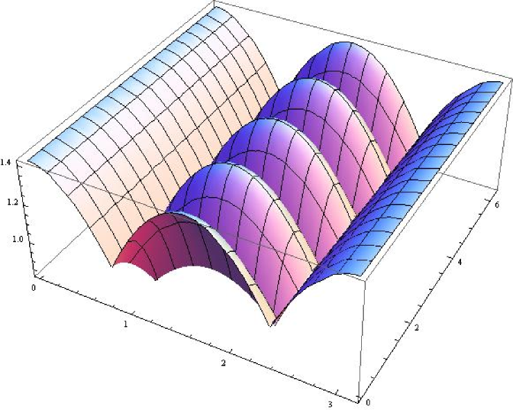
Figure 1: Surface plot of $\sqrt{g/2}$, where $0\leq\theta\leq 2\pi$ and $0\leq\varphi\leq\pi$.

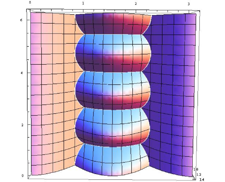
Figure 2: Another view of $\sqrt{g/2}$, with contours of intersection.