QUASIPARTICLES OF STRONGLY CORRELATED FERMI LIQUIDS AT HIGH TEMPERATURES AND IN HIGH MAGNETIC FIELDS

Аннотация

Strongly correlated Fermi systems are among the most intriguing, best experimentally studied and fundamental systems in physics. There is, however, lack of theoretical understanding in this field of physics. The ideas based on the concepts like Kondo lattice and involving quantum and thermal fluctuations at a quantum critical point have been used to explain the unusual physics. Alas, being suggested to describe one property, these approaches fail to explain the others. This means a real crisis in theory suggesting that there is a hidden fundamental law of nature. It turns out that the hidden fundamental law is well forgotten old one directly related to the Landau—Migdal quasiparticles, while the basic properties and the scaling behavior of the strongly correlated systems can be described within the framework of the fermion condensation quantum phase transition (FCQPT). The phase transition comprises the extended quasiparticle paradigm that allows us to explain the non-Fermi liquid (NFL) behavior observed in these systems. In contrast to the Landau paradigm stating that the quasiparticle effective mass is a constant, the effective mass of new quasiparticles strongly depends on temperature, magnetic field, pressure, and other parameters. Our observations are in good agreement with experimental facts and show that FCQPT is responsible for the observed NFL behavior and quasiparticles survive both high temperatures and high magnetic fields.

1 Introduction

A. B. Migdal’s contribution to modern theoretical physics is very impressive. His endowment in and deep understanding of different domains of physics, including the nuclear and many-body physics, based on Fermi-liquid approach, is outstanding. In Migdal seminal papers a solid base for studying strongly interacting Fermi systems and phase transitions occurring in them has been established mig1 ; mig2 . Migdal’s daring ideas of phase transitions related to $\pi$ condensation in nuclei and neutron stars mig2 inspired a theory of fermion condensation that has permitted to construct a new class of Fermi liquids, new quasiparticles and new type of merging of single-particle levels of both finite and infinite Fermi systems like nuclear, atomic and solid state systems ks ; ksk ; vol ; volovik2 ; merg . The new class of Fermi liquids is represented by strongly correlated Fermi systems where enormous number of experimental facts are collected. Understanding the physics of these systems stimulates intensive studies of the possible manifestation of fermion condensation in other areas, as it has happened in the case of metal superconductivity, whose ideas were successfully used in describing atomic nuclei mig1 and in a possible explanation of the origin of the mass of elementary particles. Therefore, we expect that the ideas associated with the new fermion condensation quantum phase transition prep in one area of research stimulates intensive studies of the possible manifestation of such a transition in other areas.

Strongly correlated Fermi systems represented by heavy fermion (HF) metals and quasi-two-dimensional ³He are among the most intriguing, best experimentally studied and fundamental systems in physics, which until very recently have lacked theoretical explanations prep . These are also a field never far from applications in synthesis of novel materials for cryogenics, rare earth magnets and applied superconductivity. The properties of these materials differ dramatically from those of ordinary Fermi systems prep ; ste ; varma ; vojta ; voj ; obz ; col11 . Their behavior is so unusual that the traditional Landau quasiparticles paradigm does not apply to it. The paradigm states that the properties is determined by quasiparticles whose dispersion is characterized by the effective mass $M^{*}$ which is independent of temperature $T$, the number density $x$, magnetic field $B$ and other external parameters. The above systems are, however, in defiance of theoretical understanding. The ideas based on the concepts (like Kondo lattice involving quantum and thermal fluctuations at a quantum critical point (QCP) have been used to explain the unusual physics of these systems known as non-Fermi liquid (NFL) behavior. Alas, being suggested to describe one property, these approaches fail to explain the others. This means a real crisis in theory suggesting that there is a hidden fundamental law of nature, which remains to be recognized. It is widely believed that utterly new concepts are required to describe the underlying physics. There is a fundamental question: how many concepts do we need to describe the above physical mechanisms? This cannot be answered on purely experimental or theoretical grounds. Rather, we have to use both of them. For instance, in the case of metals with heavy fermions, the strong correlation of electrons leads to a renormalization of the effective mass of quasiparticles, which may exceed the ordinary, "bare mass by several orders of magnitude or even become infinitely large at temperatures $T\to 0$. Moreover, the effective mass strongly depends on the temperature, pressure, or applied magnetic field. Such metals exhibit NFL behavior and unusual power laws of the temperature dependence of the thermodynamic properties at low temperatures.

The Landau theory of the Fermi liquid has remarkable results in describing a multitude of properties of the electron liquid in ordinary metals, Fermi liquids of the ³He type and nuclear liquid landau ; lanl1 ; migdal ; PinNoz . The theory is based on the assumption that elementary excitations determine the physics at low temperatures. These excitations behave as quasiparticles, have a certain effective mass, and, judging by their basic properties, belong to the class of quasiparticles of a weakly interacting Fermi gas. Hence, the effective mass $M^{*}$ is independent of the temperature, pressure, and magnetic field strength and is a parameter of the theory. The Landau Fermi liquid (LFL) theory fails to explain the results of experimental observations related to the dependence of $M^{*}$ on the temperature $T$, magnetic field $B$, pressure, etc.; this has led to the conclusion that quasiparticles do not survive in strongly correlated Fermi systems and that the heavy electron does not retain its identity as a quasiparticle excitation, see e.g. col11 ; col2 ; col1 .

The unusual properties and NFL behavior observed in high-$T_{c}$ superconductors, HF metals and 2D Fermi systems are assumed to be determined by various magnetic quantum phase transitions ste ; varma ; vojta ; voj ; obz ; col11 ; col2 ; geg1 . Indeed, when reasoning by analogy with respect to the second order phase transitions, one can assume that a phase transition responsible for the NFL behavior taking place up to lowest accessible temperatures is located at $T=0$. Since a quantum phase transition occurs at $T=0$, the control parameters are the composition, electron (hole) number density $x$, pressure, magnetic field strength $B$, etc. A quantum phase transition occurs at a quantum critical point, which separates the ordered phase that emerges as a result of quantum phase transition from the disordered phase. It is usually assumed that magnetic (e.g., ferromagnetic and antiferromagnetic) quantum phase transitions are responsible for the NFL behavior. The critical point of such a phase transition can be shifted to absolute zero by varying the above parameters.

Universal behavior can be expected only if the system under consideration is very close to a quantum critical point, e.g., when the correlation length is much longer than the microscopic length scale, and critical quantum and thermal fluctuations determine the anomalous contribution to the thermodynamic functions of strongly correlated Fermi system. Quantum phase transitions of this type are so widespread varma ; vojta ; voj ; col11 ; col2 that we call them ordinary quantum phase transitions shag3 . In this case, the physics of the phenomenon is determined by thermal and quantum fluctuations of the critical state, while quasiparticle excitations are destroyed by these fluctuations. Conventional arguments that quasiparticles in strongly correlated Fermi liquids "get heavy and die"at a quantum critical point commonly employ the well-known formula based on the assumptions that the $z$-factor (the quasiparticle weight in the single-particle state) vanishes at the points of second-order phase transitions col1 . However, it has been shown that this scenario is problematic khodb ; x18 .

The fluctuations in the order parameter developing an infinite correlation length and the absence of quasiparticle excitations are considered as the main reason for the NFL behavior of heavy-fermion metals, 2D fermion systems and high-$T_{c}$ superconductors vojta ; voj ; col11 ; col2 ; col3 . This approach faces certain difficulties, however. Critical behavior in experiments with metals containing heavy fermions is observed at high temperatures comparable to the effective Fermi temperature $T_{k}$. For instance, the thermal expansion coefficient $\alpha(T)$, which is a linear function of temperature for normal LFL, $\alpha(T)\propto T$, demonstrates the $\sqrt{T}$ temperature dependence in measurements involving CeNi₂Ge₂ as the temperature varies by two orders of magnitude (as it decreases from 6 K to at least 50 mK) geg1 . Such behavior can hardly be explained within the framework of the critical point fluctuation theory. Obviously, such a situation is possible only as $T\to 0$, when the critical fluctuations make the leading contribution to the entropy and when the correlation length is much longer than the microscopic length scale. At a certain temperature $T_{k}$, this macroscopically large correlation length must be destroyed by ordinary thermal fluctuations and the corresponding universal behavior must disappear.

In the rest of this paper, we show that the fermion condensation quantum phase transition (FCQPT) prep is indeed responsible for the observed fascinating NFL behavior of strongly correlated Fermi systems and quasiparticles survive both high temperatures and high magnetic fields. In Section 2, we give a detailed consideration of experimental evidences in favor of existence of quasiparticles, and formulate both a scaling behavior of strongly correlated Fermi systems and the extended quasiparticle paradigm. Then in Section 3, we consider the properties of Landau Fermi liquid. In Section 4 we demonstrate that the Landau equation for the effective is not a phenomenological one and can be derived using the methods of Density Functional Theory. Thus, we establish the extended quasiparticle paradigm. FCQPT and a phase diagram of heavy fermion system located in the vicinity of FCQPT are investigated in Section 5. We propose that the phase diagram of systems located near FCQPT are strongly influenced by control parameters such as a chemical pressure, pressure or magnetic field. We find that under the application of the chemical pressure (positive/negative) QCP is destroyed or converted into a quantum critical line, correspondingly. In Section 6 we establish that heavy fermion quasiparticles do exist in a very wide range of both temperatures $T$ and magnetic fields $B$. Finally, in Section 7 our results are summarized and discussed.

2 Experimental hints at scaling behavior and quasiparticles

There is a difficulty in explaining the restoration of the LFL behavior under the application of magnetic field $B$, as observed in HF metals and in high-$T_{c}$ superconductors ste ; geg ; cyr . For the LFL state as $T\to 0$, the electric resistivity $\rho(T)=\rho_{0}+AT^{2}$, the heat capacity $C(T)=\gamma_{0}T$, and the magnetic susceptibility $\chi=const$. It turns out that the coefficient $A(B)$, the Sommerfeld coefficient $\gamma_{0}(B)=C/T\propto M^{*}$, and the magnetic susceptibility $\chi(B)$ depend on the magnetic field strength B such that $A(B)\propto\gamma_{0}^{2}(B)$ and $A(B)\propto\chi^{2}(B)$, which implies that the Kadowaki—Woods relation $K=A(B)/\gamma_{0}^{2}(B)$ kadw is $B$-independent and is preserved geg . Such universal behavior, quite natural when quasiparticles with the effective mass $M^{*}$ playing the main role, can hardly be explained within the framework of approach that presupposes the absence of quasiparticles, which is characteristic of ordinary quantum phase transitions in the vicinity of QCP. Indeed, there is no reason to expect that $\gamma_{0}$, $\chi$ and $A$ are affected by the fluctuations in a correlated fashion.

For instance, the Kadowaki—Woods relation does not agree with the spin density wave scenario geg and with the results of research in quantum criticality based on the renormalization-group approach mill . Moreover, measurements of charge and heat transfer have shown that the Wiedemann—Franz law holds in some high-$T_{c}$ superconductors cyr ; cyr1 and HF metals pag ; pag2 ; ronn1 ; ronn . All this suggests that quasiparticles do exist in such metals, and this conclusion is also corroborated by photoemission spectroscopy results koral ; fujim .

The inability to explain the behavior of heavy-fermion metals while staying within the framework of theories based on ordinary quantum phase transitions implies that another important concept introduced by Landau, the order parameter, also ceases to operate. Thus, we are left without the most fundamental principles of many-body quantum physics landau ; lanl1 ; PinNoz , and many interesting phenomena associated with the NFL behavior of strongly correlated Fermi systems remain unexplained.

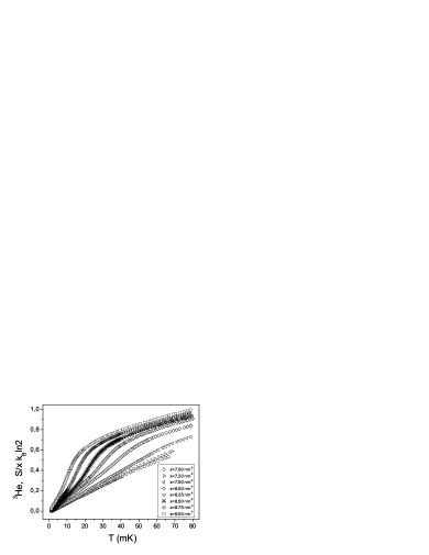
Рис. 1: The entropy of 2D $\rm{}^{3}He$ as a function of the density $x$ versus $T$ 3he . The density is depicted in the legend.

The NFL behavior manifests itself in the power-law behavior of the physical quantities of strongly correlated Fermi systems located close to their QCPs, with exponents different from those of a Fermi liquid ste ; varma ; vojta ; voj ; obz ; col11 ; col2 ; geg1 ; oesb ; steg1 ; oesbs . It is common belief that the main output of theory is the explanation of these exponents which are at least depended on the magnetic character of QCP and dimensionality of the system. On the other hand, the observed behavior of the thermodynamic properties cannot be captured by these exponents as seen from Figs. 1 —3. The behavior of the entropy $S(T)$ of two-dimensional (2D) $\rm{}^{3}He$ 3he shown in Fig. 1 is positively different from that described by a simple function $a_{1}T^{a_{2}}$ where $a_{1}$ is a constant and $a_{2}$ is the exponent. It is seen from Fig. 1 that at the low densities $x\simeq 7$ $\rm nm^{-2}$ the entropy demonstrates the LFL behavior characterized by a linear function of $T$ with $a_{2}=1$. The behavior becomes quite different at the higher densities at which $S(T)$ has an inflection point. Obviously, at the inflection point $S(T)$ cannot be fit by the simple function $a_{1}T^{a_{2}}$.

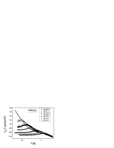
Рис. 2: Electronic specific heat of $\rm YbRh_{2}Si_{2}$, $C/T$, versus temperature $T$ as a function of magnetic field $B$ oesb shown in the legend.

As seen from Fig. 2, the specific heat $C/T$ measured on $\rm YbRh_{2}Si_{2}$ oesb exhibits a behavior that is to be described as a function of both temperature $T$ and magnetic $B$ field rather than by a single exponent. One can see that at low temperatures $C/T$ demonstrates the LFL behavior which is changed by the transition regime at which $C/T$ reaches its maximum and finally $C/T$ decays into NFL behavior as a function of $T$ at fixed $B$. It is clearly seen from Fig. 2 that, in particularly in the transition regime, these exponents may have little physical significance.

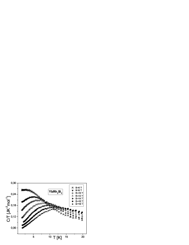
Рис. 3: The normalized effective mass $M^{*}_{N}=M^{*}/M^{*}_{M}$ versus normalized temperature $T_{N}=T/T_{M}$. $M^{*}_{N}$ is extracted from the measurements of the specific heat $C/T$ on $\rm YbRh_{2}Si_{2}$ steg1 shown in Fig. 3. The values of the field $B$ is listed in the legend.

Figure 3 displays measurements of $C/T$ on $\rm YbRh_{2}Si_{2}$ steg1 in wide range of both temperature $T$ and magnetic field $B$ variations. It is seen that both the NFL behavior and the range extends at least up to twenty Kelvins and up to 18 T. Figure 3 demonstrates that the LFL state at low temperatures and NFL one at higher temperatures are separated by the transition regime at which $C/T$ reaches its maximum value $M^{*}_{M}(B)$. Thus, we again conclude that the observed NFL behavior exhibiting the maximum and extending to high temperatures can be hardly explained in the framework of the ordinary quantum phase transitions interpreting the exponents.

In order to show that the behavior of $S$ and $C/T$ displayed in Figs. 1—3 is of generic character, we remember that in the vicinity of QCP it is helpful to use "internal"scales to measure the effective mass $M^{*}\propto C/T$ and temperature $T$ prep ; dft373 ; dftjtp . The internal scales of the thermodynamic functions such as $S$ or $C/T$ are related to "peculiar points"like the inflection or maximum. Since the entropy has no maxima, its normalization is to be performed in the inflection point taking place at $T=T_{inf}$. Note that $T_{inf}$ is a function of $x$, it is seen from Fig. 1 that the inflection point moves towards lower temperatures at elevating $x$. The normalized entropy $S_{N}$ as a function of the normalized temperature $T_{N}=T/T_{inf}=y$ is reported in Fig. 4.

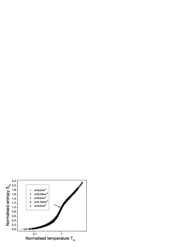
Рис. 4: The normalized entropy $S_{N}$, extracted from the experimental facts displayed in Fig. 1, as a function of $x$ shown in the legend versus normalized $T_{N}$. The arrow shows the inflection point.

We normalize the entropy by its value at the inflection point $S_{N}(y)=S(y)/S(1)$. As seen from Fig. 4, the normalization revels the scaling behavior of $S_{N}$, that is the curves at different temperatures and densities $x$ merge into a single one in terms of the variable $y$. We have excluded the experimental data taken at $x\leq 8\,{\rm nm^{-2}}$ since the corresponding curves do not contain the inflection points. It is seen from Fig. 4 that $S_{N}(y)$ extracted from the measurements is not a linear function of $y$, as would be for a LFL, and shows the scaling behavior over three decades in normalized temperature $y$.

As seen from Fig. 2, a maximum structure in $C/T\propto M^{*}_{M}$ at temperature $T_{M}$ appears under the application of magnetic field $B$ and $T_{M}$ shifts to higher $T$ as $B$ is increased. The value of the Sommerfeld coefficient $C/T=\gamma_{0}$ is saturated towards lower temperatures decreasing at elevated magnetic field. To obtain the normalized effective mass $M^{*}_{N}$, we use $M^{*}_{M}$ and $T_{M}$ as "internal"scales: The maximum structure in $C/T$ was used to normalize $C/T$, and $T$ was normalized by $T_{M}$. In Fig. 5 the normalized effective mass $M^{*}_{N}=M^{*}/M^{*}_{M}$ as a function of normalized temperature $T_{N}=T/T_{M}$ is shown by geometrical figures. Note that we have excluded the experimental data taken in magnetic field $B=0.06$ T. In that case, $T_{M}\to 0$ and the corresponding $T_{M}$ and $M^{*}_{M}$ are unavailable.

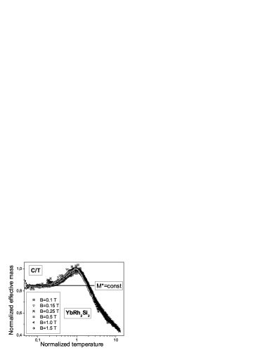
Рис. 5: The normalized effective mass $M^{*}_{N}$ versus normalized temperature $T_{N}$. $M^{*}_{N}$ is extracted from the measurements of the specific heat $C/T$ on $\rm YbRh_{2}Si_{2}$ in magnetic fields $B$ oesb listed in the legend. Constant effective mass $M^{*}_{L}$ inherent in normal Landau Fermi liquids is depicted by the solid line.

It is seen that the LFL state and NFL one are separated by the transition regime at which $M^{*}_{N}$ reaches its maximum value. Figure 5 reveals the scaling behavior of the normalized experimental curves: The curves at different magnetic fields $B$ merge into a single one in terms of the normalized variable $y=T/T_{M}$. As seen from Fig. 5, the normalized effective mass $M^{*}_{N}(y)$ extracted from the measurements is not a constant, as would be for a LFL, and shows the scaling behavior over three decades in normalized temperature $y$. It is seen from Figs. 2 and 5 that the NFL behavior and the associated scaling extend at least to temperatures up to few Kelvins.

In order to get a deep insight in the behavior of $C/T$ displayed in Fig. 3, we again use the internal scales as it was done when constructing $M^{*}_{N}$ displayed in Fig. 5. As a result, Fig. 6 reveals the scaling behavior of the normalized experimental curves: The curves at different magnetic fields $B$ merge into a single one in terms of the normalized variable $y=T/T_{M}$. As seen from Fig. 6, the normalized effective mass $M^{*}_{N}(y)$ is not a constant, as would be for a LFL, and shows the scaling behavior over two decades in normalized temperature $y$. It is seen from Figs. 3 and 6 that the NFL behavior and the associated scaling extend at least both to high temperatures up to twenty Kelvins and magnetic fields up to 18 T.

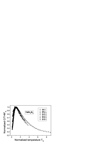
Рис. 6: The normalized effective mass $M^{*}_{N}=M^{*}/M^{*}_{M}$ versus normalized temperature $T_{N}=T/T_{M}$. $M^{*}_{N}$ is extracted from the measurements of the specific heat $C/T$ on $\rm YbRh_{2}Si_{2}$ steg1 shown in Fig. 3. The values of the field $B$ is listed in the legend.

Taking into account the scaling behavior revealed in Figs. 4—6, we conclude that a challenging problem for theories considering the NFL behavior of strongly correlated Fermi liquids is to explain both the scaling and the shape of the thermodynamic functions like $S_{N}$ and $M^{*}_{N}$. While the theories calculating only the exponents that characterize $S_{N}$ and $M^{*}_{N}$ at $y\gg 1$ deal with a part of the observed facts related to the problem and overlook, for example, consideration of the transition and LFL regimes. Another part of the problem is the remarkably large ranges of temperature, magnetic field and the density over which the NFL behavior and the scaling are observed. Concepts based on the Kondo lattice and scenarios where fluctuations in the order parameter is sufficiently big and the correlation time is sufficiently large to develop the NFL behavior can hardly match up such high temperatures and explain the observed scaling behavior.

As we will see below, the large temperature ranges are precursors of new quasiparticles, and it is the scaling behavior of the normalized effective mass that allows us to explain the thermodynamic of HF metals at the transition and NFL regimes. Taking into account the simple behavior shown in Figs. 4—6, we ask the question: what theoretical concepts can replace the Fermi-liquid paradigm with the notion of the effective mass in cases where Fermi-liquid theory breaks down? To date such a concept is not available vojta . Therefore, we focus on the concept of FCQPT preserving quasiparticles and intimately related to the unlimited growth of $M^{*}$. It was shown that it is capable of revealing the scaling behavior of the effective mass and delivering an adequate theoretical explanation of a vast majority of experimental results in different HF metals prep . In contrast to the Landau paradigm based on the assumption that $M^{*}$ is a constant as shown by the solid line in Fig. 5, in FCQPT approach the effective mass $M^{*}$ of new quasiparticles strongly depends on $T$, $x$, $B$ etc. Therefore, in accord with numerous experimental facts the extended quasiparticles paradigm is to be introduced. The main point here is that the well-defined quasiparticles determine as before the thermodynamic, relaxation and transport properties of strongly correlated Fermi-systems in large temperature ranges, while $M^{*}$ becomes a function of $T$, $x$, $B$ etc. The FCQPT approach had been already successfully applied to describe the thermodynamic properties of such different strongly correlated systems as ³He on the one hand and complicated HF compounds on the other prep ; obz ; khodb ; prl3he .

Since we are concentrated on properties that are non-sensitive to the detailed structure of the system we avoid difficulties associated with the anisotropy generated by the crystal lattice of solids, its special features, defects, etc., We study the universal behavior of strongly correlated Fermi-systems located near their QCP at low temperatures using the model of a homogeneous HF liquid dft373 ; dftjtp . The model is quite meaningful because we consider the scaling behavior exhibited by these materials at low temperatures prep . The scaling properties of the normalized effective mass that characterizes them, are determined by momentum transfers that are small compared to momenta of the order of the reciprocal lattice length. The high momentum contributions can therefore be ignored by substituting the lattice for the jelly model. While the values of the scales like the maximum $M^{*}_{M}$ of the effective mass and $T_{M}$ at which $M^{*}_{M}$ takes place are determined by a wide range of momenta and thus these scales are controlled by the specific properties of the system. On the other hand, the dependencies of these scales on magnetic fields, temperature, the density of system, pressure etc are again controlled by small momenta and can be analyzed within the model of HF liquid.

3 Normal Fermi liquids

One of the most complex problems of modern condensed matter physics is the problem of the structure and properties of Fermi systems with large inter particle coupling constants. Theory of Fermi liquids, later called "normal was first proposed by Landau as a means for solving such problems by introducing the concept of quasiparticles and amplitudes that characterize the effective quasiparticle interaction landau ; lanl1 . The Landau theory can be regarded as an effective low-energy theory with the high-energy degrees of freedom eliminated by introducing amplitudes that determine the quasiparticle interaction instead of the strong inter particle interaction. The stability of the ground state of the Landau Fermi liquid is determined by the Pomeranchuk stability conditions: stability is violated when at least one Landau amplitude becomes negative and reaches its critical value landau ; lanl1 ; pom . We note that the new phase in which stability is restored can also be described, in principle, by the LFL theory.

We begin by recalling the main ideas of the LFL theory landau ; lanl1 ; PinNoz . The theory is based on the quasiparticle paradigm, which states that quasiparticles are elementary weakly excited states of Fermi liquids and are therefore specific excitations that determine the low-temperature thermodynamic and transport properties of Fermi liquids. In the case of the electron liquid, the quasiparticles are characterized by the electron quantum numbers and the effective mass $M^{*}$. The ground state energy of the system is a functional of the quasiparticle occupation numbers (or the quasiparticle distribution function) $n({\bf p},T)$, and the same is true of the free energy $F(n({\bf p},T))$, the entropy $S(n({\bf p},T))$, and other thermodynamic functions. We can find the distribution function from the minimum condition for the free energy $F=E-TS$ (here and in what follows $k_{B}=\hbar=1$)

$$\frac{\delta(F-\mu N)}{\delta n({\bf p},T)}=\varepsilon({\bf p},T)-\mu(T)-T\ln\frac{1-n({\bf p},T)}{n({\bf p},T)}=0.$$ (1)

Here $\mu$ is the chemical potential fixing the number density

$$x=\int n({\bf p},T)\frac{d{\bf p}}{(2\pi)^{3}},$$ (2)

and

$$\varepsilon({\bf p},T)\ =\ \frac{\delta E(n({\bf p},T))}{\delta n({\bf p},T)}\,$$ (3)

is the quasiparticle energy. This energy is a functional of $n({\bf p},T)$, in the same way as the energy $E$ is: $\varepsilon({\bf p},T,n)$. The entropy $S(n({\bf p},T))$ related to quasiparticles is given by the well-known expression landau ; lanl1

$$S(n({\bf p},T)) = -2\int[n({\bf p},T)\ln(n({\bf p},T))+(1-n({\bf p},T))$$ (4)

$$\times \ln(1-n({\bf p},T))]\frac{d{\bf p}}{(2\pi)^{3}},$$

which follows from combinatorial reasoning. Equation (1) is usually written in the standard form of the Fermi—Dirac distribution,

$$n({\bf p},T)=\left\{1+\exp\left[\frac{(\varepsilon({\bf p},T)-\mu)}{T}\right]\right\}^{-1}.$$ (5)

At $T\to 0$, (1) and (5) have the standard solution $n(p,T\to 0)\to\theta(p_{f}-p)$ if the derivative $\partial\varepsilon(p\simeq p_{\rm F})/\partial p$ is finite and positive. Here $p_{\rm F}$ is the Fermi momentum and $\theta(p_{\rm F}-p)$ is the step function. The single particle energy can be approximated as $\varepsilon(p\simeq p_{\rm F})-\mu\simeq p_{\rm F}(p-p_{\rm F})/M^{*}_{L}$, and $M^{*}_{L}$ inversely proportional to the derivative is the effective mass of the Landau quasiparticle,

$$\frac{1}{M^{*}_{L}}=\frac{1}{p}\,\frac{d\varepsilon(p,T=0)}{dp}|_{p=p_{\rm F}}\ .$$ (6)

In turn, the effective mass $M^{*}_{L}$ is related to the bare electron mass $m$ by the well-known Landau equation landau ; lanl1 ; PinNoz

$$\frac{1}{M^{*}_{L}} = \frac{1}{m}+\sum_{\sigma_{1}}\int\frac{{\bf p}_{F}{\bf p_{1}}}{p_{\rm F}^{3}}F_{\sigma,\sigma_{1}}({\bf p_{\rm F}},{\bf p}_{1})$$ (7)

$$\times \frac{\partial n_{\sigma_{1}}({\bf p}_{1},T)}{\partial{p}_{1}}\frac{d{\bf p}_{1}}{(2\pi)^{3}}.$$

where $F_{\sigma,\sigma_{1}}({\bf p_{\rm F}},{\bf p}_{1})$ is the Landau amplitude, which depends on the momenta ${\bf p_{\rm F}}$ and ${\bf p}$ and the spins $\sigma$. For simplicity, we ignore the spin dependence of the effective mass, because $M^{*}_{L}$ is almost completely spin-independent in the case of a homogeneous liquid and weak magnetic fields. The Landau amplitude $F$ is given by

$$F_{\sigma,\sigma_{1}}({\bf p},{\bf p}_{1},n)=\frac{\delta^{2}E(n)}{\delta n_{\sigma}({\bf p})\delta n_{\sigma_{1}}({\bf p}_{1})}.$$ (8)

The stability of the ground state of LFL is determined by the Pomeranchuk stability conditions: stability is violated when at least one Landau amplitude becomes negative and reaches its critical value lanl1 ; PinNoz ; pom

$$F^{a,s}_{L}=-(2L+1).$$ (9)

Here $F^{a}_{L}$ and $F^{s}_{L}$ are the dimensionless spin-symmetric and spin-antisymmetric Landau amplitudes, $L$ is the angular momentum related to the corresponding Legendre polynomials $P_{L}$,

$$F({\bf p\sigma},{\bf p}_{1}\sigma_{1})=\frac{1}{N}\sum^{\infty}_{L=0}P_{L}(\Theta)\left[F^{a}_{L}\sigma,\sigma_{1}+F^{s}_{L}\right].$$ (10)

Here $\Theta$ is the angle between momenta ${\bf p}$ and ${\bf p}_{1}$ and the density of states $N=M^{*}_{L}p_{\rm F}/(2\pi^{2})$. It follows from Eq. (7) that

$$\frac{M^{*}_{L}}{m}=1+\frac{F^{s}_{1}}{3}.$$ (11)

In accordance with the Pomeranchuk stability conditions it is seen from Eq. (11) that $F^{s}_{1}>-3$, otherwise the effective mass becomes negative leading to unstable state when it is energetically favorable to excite quasiparticles near the Fermi surface.

4 Effective mass and scaling behavior

It is common belief that the equations of the Section 3 are phenomenological and inapplicable to describe Fermi systems characterized by the effective mass $M^{*}$ strongly dependent on temperature, external magnetic fields $B$, pressure $P$ etc. To derive the equation determining the effective mass, we consider the model of a homogeneous HF liquid and employ the density functional theory for superconductors (SCDFT) gross which allows us to consider $E$ as a functional of the occupations numbers $n({\bf p})$ dft373 ; dft ; dft269 ; sh . As a result, the ground state energy of the normal state $E$ becomes the functional of the occupation numbers and the function of the number density $x$, $E=E(n({\bf p}),x)$, while Eq. (3) gives the single-particle spectrum. Upon differentiating both sides of Eq. (3) with respect to ${\bf p}$ and after some algebra and integration by parts, we obtain khodb ; dft373 ; dft ; dft269

$$\frac{\partial\varepsilon({\bf p})}{\partial{\bf p}}=\frac{{\bf p}}{m}+\int F({\bf p},{\bf p}_{1},n)\frac{\partial n({\bf p}_{1})}{\partial{\bf p}_{1}}\frac{d{\bf p}_{1}}{(2\pi)^{3}}.$$ (12)

To calculate the derivative $\partial\varepsilon({\bf p})/\partial{\bf p}$, we employ the functional representation

$$E(n) = \int\frac{p^{2}}{2m}n({\bf p})\frac{d{\bf p}}{(2\pi)^{3}}$$ (13)

$$+ \frac{1}{2}\int F({\bf p},{\bf p}_{1},n)_{|_{n=0}}\,n({\bf p})n({\bf p}_{1})\frac{d{\bf p}d{\bf p}_{1}}{(2\pi)^{6}}+...$$

It is seen directly from Eq. (12) that the effective mass is given by the well-known Landau equation

$$\frac{1}{M^{*}}=\frac{1}{m}+\int\frac{{\bf p}_{F}{\bf p_{1}}}{p_{\rm F}^{3}}F({\bf p_{\rm F}},{\bf p}_{1},n)\frac{\partial n(p_{1})}{\partial p_{1}}\frac{d{\bf p}_{1}}{(2\pi)^{3}}.$$ (14)

For simplicity, we ignore the spin dependencies. To calculate $M^{*}$ as a function of $T$, we construct the free energy $F=E-TS$, where the entropy $S$ is given by Eq. (4). Minimizing $F$ with respect to $n({\bf p})$, we arrive at the Fermi—Dirac distribution, Eq. (5). Due to the above derivation, we conclude that Eqs. (12) and (14) are exact ones and allow us to calculate the behavior of both $\partial\varepsilon({\bf p})/\partial{\bf p}$ and $M^{*}$ which now is a function of temperature $T$, external magnetic field $B$, number density $x$ and pressure $P$ rather than a constant. As we will see it is this feature of $M^{*}$ that forms both the scaling and the NFL behavior observed in measurements on HF metals.

In LFL theory it is assumed that $M^{*}_{L}$ is positive, finite and constant since the integral on the right hand side of Eq. (14) represents a small correction in the case of normal metals. As a result, the temperature-dependent corrections to $M^{*}_{L}$, the quasiparticle energy $\varepsilon({\bf p})$ and other quantities begin with the term proportional to $T^{2}$ in 3D systems and with the term proportional to $T$ in 2D one chub . The effective mass is given by Eq. (7), and the specific heat $C$ is landau

$$C=\frac{2\pi^{2}NT}{3}=\gamma_{0}T=T\frac{\partial S}{\partial T},$$ (15)

and the spin susceptibility

$$\chi=\frac{3\gamma_{0}\mu_{B}^{2}}{\pi^{2}(1+F^{a}_{0})},$$ (16)

where $\mu_{B}$ is the Bohr magneton and $\gamma_{0}\propto M^{*}_{L}$. In the case of LFL the electrical resistivity at low $T$ is given by PinNoz

$$\rho(T)=\rho_{0}+AT^{2},$$ (17)

where $\rho_{0}$ is the residual resistivity and $A$ is the coefficient determining the charge transport. The coefficient $A$ is proportional to the quasiparticle-quasiparticle scattering cross-section. Equation (17) symbolizes and defines the LFL behavior observed in normal metals.

Equation (14) at $T=0$, combined with the fact that $n({\bf p},T=0)$ becomes $\theta(p_{\rm F}-p)$, yields the well-known result vollh ; pfw ; vollh1

$$\frac{M^{*}}{m}=\frac{1}{1-f_{N}^{1}/3}.$$

where $f_{N}^{1}=N_{0}f^{1}$, $N_{0}=mp_{\rm F}/(2\pi^{2})$ is the density of states of a free Fermi gas and $f^{1}(p_{\rm F},p_{\rm F})$ is the $p$-wave component of the Landau interaction amplitude. Because $x=p_{\rm F}^{3}/3\pi^{2}$ in the Landau Fermi-liquid theory, the Landau interaction amplitude can be written as $f_{N}^{1}(p_{\rm F},p_{\rm F})=f_{N}^{1}(x)$. Provided that at a certain critical point $x_{\rm FC}$, the denominator $(1-f_{N}^{1}(x)/3)$ tends to zero, i.e., $(1-f_{N}^{1}(x)/3)\propto(x-x_{\rm FC})+a(x-x_{\rm FC})^{2}+...\to 0$, we find that khod1 ; shag1

$$\frac{M^{*}(x)}{m}\simeq a_{1}+\frac{a_{2}}{x-x_{\rm FC}}\propto\frac{1}{r}.$$ (18)

where $a_{1}$ and $a_{2}$ are constants and $r=(x-x_{\rm FC})/x_{\rm FC}$ is the ‘‘distance’’ from QCP $x_{\rm FC}$ at which $M^{*}(x\to x_{\rm FC})\to\infty$. We note that the divergence of the effective mass given by Eq. (18) does preserve the Pomeranchuk stability conditions for $f_{N}^{1}$ is positive, see Eq. (9). Equations (11) and (18) seem to be different but it is not the case since $f_{N}^{1}\propto m$, while $F^{s}_{1}\propto M^{*}$ and Eq. (11) represents an implicit formula for the effective mass.

The behavior of $M^{*}(x)$ described by formula (18) is in good agreement with the results of experiments cas1 ; skdk ; skdk1 and calculations krot ; sarm1 ; sarm2 . In the case of electron systems, Eq. (18) holds for $x>x_{\rm FC}$, while for 2D ³He we have $x<x_{\rm FC}$ so that always $r>0$ ksk ; ksz . Such behavior of the effective mass is observed in HF metals, which have a fairly flat and narrow conductivity band corresponding to a large effective mass, with a strong correlation and the effective Fermi temperature $T_{k}\sim p_{\rm F}^{2}/M^{*}(x)$ of the order of several dozen degrees kelvin or even lower (e.g., see Ref. ste ).

The effective mass as a function of the electron density $x$ in a silicon MOSFET (Metal Oxide Semiconductor Field Effect Transistor), approximated by Eq. (18), is shown in Fig. 7. The parameters $a_{1}$, $a_{2}$ and $x_{\rm FC}$ are taken as fitting. We see that Eq. (18) provides a good description of the experimental results.

Рис. 7: The ratio $M^{*}/M$ in a silicon MOSFET as a function of the electron number density $x$. The squares mark the experimental data on the Shubnikov-de Haas oscillations, and the data obtained by applying a parallel magnetic field are marked by circles skdk ; skdk1 ; krav . The solid line represents the function (18).

The divergence of the effective mass $M^{*}(x)$ discovered in measurements involving 2D ³He cas1 ; krav ; cas is illustrated in Fig. 8. Figures 7 and 8 show that the description provided by Eq. (18) does not depend on elementary Fermi particles constituting the system and is in good agreement with the experimental data.

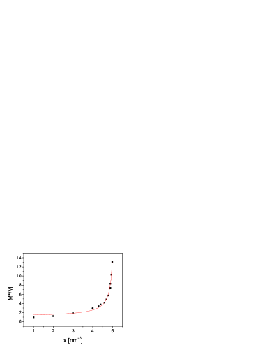
Рис. 8: The ratio $M^{*}/M$ in 2D ³He as a function of the density $x$ of the liquid, obtained from heat capacity and magnetization measurements. The experimental data are marked by squares cas1 ; cas , and the solid line represents the function given by Eq. (18).

It is instructive to briefly explore the scaling behavior of $M^{*}$ in order to illustrate the ability of the quasiparticle extended paradigm to capture the scaling behavior. Let us write the quasiparticle distribution function as $n_{1}({\bf p})=n({\bf p},T)-n({\bf p})$, with $n({\bf p})$ being the step function, and Eq. (14) then becomes

$$\frac{1}{M^{*}(T)}=\frac{1}{M^{*}}+\int\frac{{\bf p}_{F}{\bf p_{1}}}{p_{\rm F}^{3}}F({\bf p_{\rm F}},{\bf p}_{1})\frac{\partial n_{1}(p_{1},T)}{\partial p_{1}}\frac{d{\bf p}_{1}}{(2\pi)^{3}}.$$ (19)

At QCP $x\to x_{\rm FC}$, the effective mass $M^{*}(x)$ diverges and Eq. (19) becomes homogeneous determining $M^{*}$ as a function of temperature while the system exhibits the NFL behavior. If the system is located before QCP, $M^{*}$ is finite, at low temperatures the integral on the right hand side of Eq. (19) represents a small correction to $1/M^{*}$ and the system demonstrates the LFL behavior seen in Figs. 2 and 5. The LFL behavior assumes that the effective mass is independent of temperature, $M^{*}(T)\simeq const$, as shown by the horizontal line in Fig. 5. Obviously, the LFL behavior takes place only if the second term on the right hand side of Eq. (19) is small in comparison with the first one. Then, as temperature rises the system enters the transition regime: $M^{*}$ grows, reaching its maximum $M^{*}_{M}$ at $T=T_{M}$, with subsequent diminishing. As seen from Fig. 5, near temperatures $T\geq T_{M}$ the last "traces"of LFL regime disappear, the second term starts to dominate, and again Eq. (19) becomes homogeneous, and the NFL behavior is restored, manifesting itself in decreasing $M^{*}$ as a function of $T$.

5 Fermion condensation quantum phase transition

As shown in Section 4, the Pomeranchuk stability conditions do not encompass all possible types of instabilities and that at least one related to the divergence of the effective mass given by Eq. (18) was overlooked ks . This type of instability corresponds to a situation where the effective mass, the most important characteristic of quasiparticles, can become infinitely large. As a result, the quasiparticle kinetic energy is infinitely small near the Fermi surface and the quasiparticle distribution function $n({\bf p})$ minimizing $E(n({\bf p}))$ is determined by the potential energy. This leads to the formation of a new class of strongly correlated Fermi liquids with FC ks ; ksk ; vol_1 ; volovik2 ; vol , separated from the normal Fermi liquid by FCQPT shag3 ; ms ; shb ; sh1 .

It follows from (18) that at $T=0$ and as $r\to 0$ the effective mass diverges, $M^{*}(r)\to\infty$. Beyond the critical point $x_{\rm FC}$, the distance $r$ becomes negative and, correspondingly, so does the effective mass. To avoid an unstable and physically meaningless state with a negative effective mass, the system must undergo a quantum phase transition at the critical point $x=x_{\rm FC}$, which, as we will see shortly, is FCQPT ms ; shb ; sh1 ; shag3 . Because the kinetic energy of quasiparticles that are near the Fermi surface is proportional to the inverse effective mass, the potential energy of the quasiparticles near the Fermi surface determines the ground-state energy as $x\to x_{\rm FC}$. Hence, at $T=0$ a phase transition reduces the energy of the system and transforms the quasiparticle distribution function. Beyond QCP $x=x_{\rm FC}$, the quasiparticle distribution is determined by the ordinary equation for a minimum of the energy functional ks :

$$\frac{\delta E(n({\bf p}))}{\delta n({\bf p})}=\varepsilon({\bf p})=\mu;\,p_{i}\leq p\leq p_{\rm F}.$$ (20)

Equation (20) yields the quasiparticle distribution function $n_{0}({\bf p})$ that minimizes the ground-state energy $E$. This function found from Eq. (20) differs from the step function in the interval from $p_{i}$ to $p_{\rm F}$, where $0<n_{0}({\bf p})<1$, and coincides with the step function outside this interval. In fact, Eq. (20) coincides with Eq. (3) provided that the Fermi surface at $p=p_{\rm F}$ transforms into the Fermi volume at $p_{i}\leq p\leq p_{f}$ suggesting that the single-particle spectrum is absolutely ‘‘flat’’ within this interval. A possible solution $n_{0}({\bf p})$ of Eq. (20) and the corresponding single-particle spectrum $\varepsilon({\bf p})$ are depicted in Fig. 9. Quasiparticles with momenta within the interval $(p_{f}-p_{i})$ have the same single-particle energies equal to the chemical potential $\mu$ and form FC, while the distribution $n_{0}({\bf p})$ describes the new state of the Fermi liquid with FC ks ; ksk ; vol . In contrast to the Landau, marginal, or Luttinger Fermi liquids varma , which exhibit the same topological structure of the Green’s function, in systems with FC, where the Fermi surface spreads into a strip, the Green’s function belongs to a different topological class. The topological class of the Fermi liquid is characterized by the invariant

Рис. 9: The single-particle spectrum $\varepsilon(p)$ and the quasiparticle distribution function $n_{0}(p)$. Because $n_{0}(p)$ is a solution of Eq. (20) at $T=0$, we have $n_{0}(p<p_{i})=1$, $0<n_{0}(p_{i}<p<p_{f})<1$, and $n_{0}(p>p_{f})=0$, while $\varepsilon(p_{i}<p<p_{f})=\mu$ and the band becomes completely flat. The Fermi momentum $p_{\rm F}$ satisfies the condition $p_{i}<p_{\rm F}<p_{f}$.

volovik1 ; volovik2 ; vol

$$N=tr\oint_{C}\frac{dl}{2\pi i}G(i\omega,{\bf p})\partial_{l}G^{-1}(i\omega,{\bf p}),$$ (21)

where ‘‘tr’’ denotes the trace over the spin indices of the Green’s function and the integral is taken along an arbitrary contour $C$ encircling the singularity of the Green’s function. The invariant $N$ in (21) takes integer values even when the singularity is not of the pole type, cannot vary continuously, and is conserved in a transition from the Landau Fermi liquid to marginal liquids and under small perturbations of the Green’s function. As shown by Volovik volovik1 ; volovik2 ; vol , the situation is quite different for systems with FC, where the invariant $N$ becomes a half-integer and the system with FC transforms into an entirely new class of Fermi liquids with its own topological structure.

Phase diagram of Fermi system with FCQPT

We start with visualizing the main properties of FCQPT. To this end, again consider SCDFT. SCDFT states that the thermodynamic potential $\Phi$ is a universal functional of the number density $n({\bf r})$ and the anomalous density (or the order parameter) $\kappa({\bf r},{\bf r}_{1})$, providing a variational principle to determine the densities. At the superconducting transition temperature $T_{c}$ a superconducting state undergoes the second order phase transition. Our goal now is to construct a quantum phase transition which evolves from the superconducting one, since, as seen from Fig. 9, the superconducting order parameter $\kappa(p)=\sqrt{n(p)(1-n(p))}$ is finite over the region $(p_{f}-p_{i})$.

Let us assume that the coupling constant $\lambda_{0}$ of the BCS-like pairing interaction bcs vanishes, with $\lambda_{0}\to 0$ making vanish the superconducting gap at any finite temperature. In that case, $T_{c}\to 0$ and the superconducting state takes place at $T=0$ while at finite temperatures there is a normal state. This means that at $T=0$ the anomalous density

$$\kappa({\bf r},{\bf r_{1}})=\langle\Psi\uparrow({\bf r})\Psi\downarrow({\bf r_{1}})\rangle$$ (22)

is finite, while the superconducting gap

$$\Delta({\bf r})=\lambda_{0}\int\kappa({\bf r},{\bf r_{1}})d{\bf r_{1}}$$ (23)

is infinitely small obz ; shag1 . In Eq. (22), the field operator $\Psi_{\sigma}({\bf r})$ annihilates an electron of spin $\sigma,\sigma=\uparrow,\downarrow$ at the position ${\bf r}$. For the sake of simplicity, we consider the model of homogeneous HF liquid obz . Then at $T=0$, the thermodynamic potential $\Phi$ reduces to the ground state energy $E$ which turns out to be a functional of the occupation number $n({\bf p})$ since in that case the order parameter $\kappa({\bf p})=v({\bf p})u({\bf p})=\sqrt{n({\bf p})(1-n({\bf p}))}$. Indeed,

$$n({\bf p})=v^{2}({\bf p});\,\,\,\kappa({\bf p})=v({\bf p})u({\bf p}),$$ (24)

where $u({\bf p})$ and $v({\bf p})$ are normalized parameters such that $v^{2}({\bf p})+u^{2}({\bf p})=1$ and $\kappa({\bf p})=\sqrt{n({\bf p})(1-n({\bf p}))}$, see e.g. lanl1 .

Upon minimizing $E$ with respect to $n({\bf p})$, we obtain Eq. (20). As soon as Eq. (20) has nontrivial solution $n_{0}({\bf p})$ then instead of the Fermi step, we have $0<n_{0}({\bf p})<1$ in certain range of momenta $p_{i}\leq p\leq p_{\rm F}$ with $\kappa({\bf p})=\sqrt{n_{0}({\bf p})(1-n_{0}({\bf p}))}$ being finite in this range, while the single particle spectrum $\varepsilon({\bf p})$ is flat. Thus, the step-like Fermi filling inevitably undergoes restructuring and forms FC when Eq. (20) possesses for the first time the nontrivial solution at $x=x_{c}$ which is QCP of FCQPT. In that case, the range vanishes, $p_{i}\to p_{f}\to p_{\rm F}$, and the effective mass $M^{*}$ diverges at QCP obz ; khodb ; ks

$$\frac{1}{M^{*}(x\to x_{c})}=\frac{1}{p_{\rm F}}\frac{\partial\varepsilon({\bf p})}{\partial{\bf p}}|_{p\to p_{\rm F};\,x\to x_{c}}\to 0.$$ (25)

At any small but finite temperature the anomalous density $\kappa$ (or the order parameter) decays and this state undergoes the first order phase transition and converts into a normal state characterized by the thermodynamic potential $\Phi_{0}$. Indeed, at $T\to 0$, the entropy $S=-\partial\Phi_{0}/\partial T$ of the normal state is given by Eq. (4). It is seen from Eq. (4) that the normal state is characterized by the temperature-independent entropy $S_{0}$ obz ; khodb ; yakov . Since the entropy of the superconducting ground state is zero, we conclude that the entropy is discontinuous at the phase transition point, with its discontinuity $\delta S=S_{0}$. Thus, the system undergoes the first order phase transition. The heat $q$ of transition from the asymmetrical to the symmetrical phase is $q=T_{c}S_{0}=0$ since $T_{c}=0$. Because of the stability condition at the point of the first order phase transition, we have $\Phi_{0}(n({\bf p}))=\Phi(\kappa({\bf p}))$. Obviously the condition is satisfied since $q=0$.

At $T=0$, a quantum phase transition is driven by a nonthermal control parameter, e.g., the number density $x$. As we have seen in Section 4, at QCP, $x=x_{\rm FC}$, the effective mass diverges. It follows from Eq. (18) that beyond QCP, the effective mass becomes negative. To avoid an unstable and physically meaningless state with a negative effective mass, the system undergoes FCQPT leading to the formation of FC.

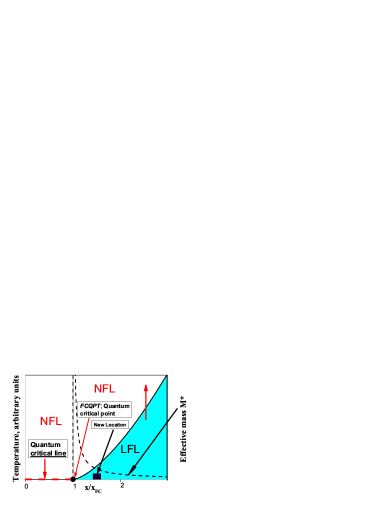
Рис. 10: Schematic phase diagram of system with FC. The number density $x$ is taken as the control parameter and depicted as $x/x_{\rm FC}$. The dashed line shows $M^{*}(x/x_{\rm FC})$ as the system approaches QCP, $x/x_{\rm FC}=1$, of FCQPT which is denoted by the arrow. At $x/x_{\rm FC}>1$ and sufficiently low temperatures, the system is in the LFL state as shown by the shadow area. The new location of the system induced by the application of the positive pressure is shown by both the solid square and the arrow. The vertical arrow illustrates the system moving in the LFL-NFL direction along $T$ at fixed control parameter. At $T=0$ and beyond the critical point, $x/x_{\rm FC}<1$, the system is at the quantum critical line depicted by the dashed line and shown by the vertical arrow. The critical line is characterized by the FC state with finite superconducting order parameter $\kappa$. At any finite low temperature $T>T_{c}=0$, $\kappa$ is destroyed, the system undergoes the first order phase transition, possesses finite entropy $S_{0}$ and exhibits the NFL behavior at any finite temperatures $T<T_{f}$.

A schematic phase diagram of the system which is driven to the FC state by variation of $x$ is reported in Fig. 10. Upon approaching the critical density $x_{\rm FC}$ the system remains in the LFL region at sufficiently low temperatures as it is shown by the shadow area. The temperature range of the shadow area shrinks as the system approaches QCP, and $M^{*}(x/x_{\rm FC})$ diverges as shown by the dashed line and Eq. (18). At QCP $x_{\rm FC}$ shown by the arrow in Fig. 10, the system demonstrates the NFL behavior down to the lowest temperatures. Beyond the critical point at finite temperatures the behavior remains the NFL and is determined by the temperature-independent entropy $S_{0}$ obz ; yakov . In that case at $T\to 0$, the system is again demonstrating the NFL behavior and approaching a quantum critical line (QCL) (shown by the vertical arrow and the dashed line in Fig. 10) rather than a quantum critical point. Upon reaching the quantum critical line from the above at $T\to 0$ the system undergoes the first order quantum phase transition, which is FCQPT taking place at $T_{c}=0$. While at diminishing temperatures, the systems located before QCP do not undergo a phase transition and their behavior transits from NFL to LFL.

It is seen from Fig. 10 that at finite temperatures there is no boundary (or phase transition) between the states of systems located before or behind QCP shown by the arrow. Therefore, at elevated temperatures the properties of systems with $x/x_{\rm FC}<1$ or with $x/x_{\rm FC}>1$ become indistinguishable. On the other hand, at $T>0$ the NFL state above the critical line and in the vicinity of QCP is strongly degenerate, therefore the degeneracy stimulates the emergence of different phase transitions lifting it and the NFL state can be captured by the other states such as superconducting (for example, by the superconducting state (SC) in $\rm CeCoIn_{5}$ shag1 ; yakov ) or by antiferromagnetic (AF) state (e.g. AF one in $\rm YbRh_{2}Si_{2}$ dft373 ) etc. The diversity of phase transitions occurring at low temperatures is one of the most spectacular features of the physics of many HF metals. Within the scenario of ordinary quantum phase transitions, it is hard to understand why these transitions are so different from one another and their critical temperatures are so extremely small. However, such diversity is endemic to systems with a FC khodb .

As mentioned above, the system located above QCL exhibits the NFL behavior down to lowest temperatures unless it is captured by a phase transition. The behavior exhibiting by the system located above QCL is in accordance with the experimental observations that study the evolution of QCP in $\rm YbRh_{2}Si_{2}$ under negative chemical pressure induced with $\rm Ir/Ge$ substitution stegnat ; steg2 . As reported, the negative pressure leaves an intermediate spin-liquid-type ground state over a finite magnetic field range. We assume a simple model that the application of negative pressure reduces $x$ and the system moves to a position over QCL. That is the $\rm Ir/Ge$ substitution drives $\rm YbRh_{2}Si_{2}$ to a paramagnetic state over the finite magnetic field $B$ range, so that the electronic system of the HF metal is located above QCL shown in Fig. 10 and demonstrates the NFL behavior. In that case magnetic field $B$ represents an additional control parameter driving $\rm YbRh_{2}Si_{2}$ to the paramagnetic state. We predict that at lowering temperatures, the electronic system of $\rm YbRh_{2}Si_{2}$ is captured by a phase transition, since the NFL state above QCL is strongly degenerate. At diminishing temperatures, this degeneracy is to be removed by some phase transition which likely can be detected by the LFL state accompanying it.

Upon using nonthermal tuning parameters like the number density $x$, the NFL behavior can be destroyed and the LFL one will be restored. In our simple model, the application of positive pressure $P$ makes $x$ grow removing the QCP of FCQPT shown in Fig. 10, so that the electronic system of $\rm YbRh_{2}Si_{2}$ moves into the shadow area characterized by the LFL behavior at low temperatures. The new location of the system is shown by the arrow pointing at the solid square. As a result, the application of magnetic field $B\simeq B_{c0}$ does not drive the system to its QCP with the divergent effective mass because the QCP is already destroyed by the pressure. Here $B_{c0}$ is the critical magnetic field that eliminates the corresponding AF order. At $B>B_{c0}$ and raising temperatures, the system moving along the vertical arrow transits from the LFL regime to the NFL one. As seen from Fig. 10, in the NFL regime the system properties coincide with that of the system at $P=0$. The observed behavior is in accord with the experimental facts indicating the separation of the AF order from QCP under the application of pressure in $\rm YbRh_{2}Si_{2}$ stegjap .

6 High magnetic fields thermodynamics of heavy fermion quasiparticles

As was mentioned in Section 2, one of the most interesting and puzzling issues in the research of HF metals is the NFL behavior taking place in wide range of both temperature $T$ and magnetic field $B$ variations hmbt . For example, measurements of the specific heat on $\rm YbRh_{2}Si_{2}$ under the application of magnetic field $B$ show that the range extends at least up to twenty Kelvins as shown in Fig. 3. In Fig. 6 the normalized effective mass $M^{*}_{N}$ as a function of normalized temperature $T_{N}$ is shown by geometrical figures. Figures 3 and 6 reveal the remarkably large temperature ranges over which the NFL behavior and scaling one are observed.

In this Section, we analyze the thermodynamic properties of $\rm YbRh_{2}Si_{2}$ in both low and high magnetic fields. Our calculations of the specific heat and magnetization allow us to conclude that under the application of magnetic field the heavy-electron system of $\rm YbRh_{2}Si_{2}$ evolves continuously without a metamagnetic transition. At low temperatures and high magnetic fields $B\simeq B^{*}$ the system is completely polarized and demonstrates the LFL behavior, at elevated temperatures the HF behavior and related NFL one are restored. The obtained results are in good agreement with experimental facts as both temperature and magnetic field vary by more than two orders of magnitude.

We use the Landau equation (14) to study the behavior of the effective mass $M^{*}(T,B)$ as a function of the temperature and the magnetic field. For the model of homogeneous HF liquid at finite temperatures and magnetic fields, Eq. (14) acquires the form landau ; prep

$$\frac{1}{M^{*}_{\sigma}(T,B)} = \frac{1}{m}+\sum_{\sigma_{1}}\int\frac{{\bf p}_{F}{\bf p}}{p_{\rm F}^{3}}F_{\sigma,\sigma_{1}}({\bf p_{\rm F}},{\bf p})$$ (26)

$$\times \frac{\partial n_{\sigma_{1}}({\bf p},T,B)}{\partial{p}}\frac{d{\bf p}}{(2\pi)^{3}}.$$

where $F_{\sigma,\sigma_{1}}({\bf p_{\rm F}},{\bf p})$ is the Landau amplitude dependent on momenta $p_{\rm F}$, $p$ and spin $\sigma$. For the sake of definiteness, we assume that the HF liquid is 3D liquid. The quasiparticle distribution function can be expressed as

$$n_{\sigma}({\bf p},T)=\left\{1+\exp\left[\frac{(\varepsilon_{\sigma}({\bf p},T)-\mu_{\sigma})}{T}\right]\right\}^{-1},$$ (27)

where $\varepsilon_{\sigma}({\bf p},T)$ is the single-particle spectrum. In our case, the chemical potential may depend on the spin due to the Zeeman splitting $\mu_{\sigma}=\mu\pm\mu_{B}B$, where $\mu_{B}$ is the Bohr magneton and $\mu$ is the chemical potential preserving the number of particles. We write the quasiparticle distribution function as $n_{\sigma}({\bf p},T,B)\equiv\delta n_{\sigma}({\bf p},T,B)+n_{\sigma}({\bf p},T=0,B=0)$. Equation (26) then becomes

$$\frac{1}{M^{*}(T,B)}=\frac{1}{M^{*}}+\frac{1}{p_{\rm F}^{2}}\sum_{\sigma_{1}}\int\frac{{\bf p}_{F}{\bf p_{1}}}{p_{\rm F}}$$ (28)

$$\times F_{\sigma,\sigma_{1}}({\bf p_{\rm F}},{\bf p}_{1})\frac{\partial\delta n_{\sigma_{1}}({\bf p}_{1},T,B)}{\partial{p}_{1}}\frac{d{\bf p}_{1}}{(2\pi)^{3}}.$$

Equation (28) is solved with a quite general form of Landau interaction amplitude ckhz . Choice of the amplitude is dictated by the fact that the system has to be at the quantum critical point of FCQPT, which means that the first two $p$-derivatives of the single-particle spectrum $\varepsilon({\bf p})$ should equal zero. Since the first derivative is proportional to the reciprocal quasiparticle effective mass $1/M^{*}$, its zero just signifies QCP of FCQPT. The second derivative must vanish; otherwise $\varepsilon(p)-\mu$ has the same sign below and above the Fermi surface, and the Landau state becomes unstable khodb ; prep . Zeros of these two subsequent derivatives mean that the spectrum $\varepsilon({\bf p})$ has an inflection point at $p_{\rm F}$ so that the lowest term of its Taylor expansion is proportional to $(p-p_{\rm F})^{3}$.

When the system is near FCQPT, it turns out that the normalized solution of Eq. (28) $M^{*}_{N}(y)$ can be well approximated by a simple universal interpolating function. The interpolation occurs between the LFL ($M^{*}\propto a+bT^{2}$) and NFL ($M^{*}\propto T^{-2/3}$) regimesprep

$$M^{*}_{N}(y)\approx c_{0}\frac{1+c_{1}y^{2}}{1+c_{2}y^{8/3}}.$$ (29)

Here $a$ and $b$ are constants, $c_{0}=(1+c_{2})/(1+c_{1})$, $c_{1}$ and $c_{2}$ are fitting parameters, related to the Landau amplitude. Magnetic field $B$ enters Eq. (27) as $B\mu_{B}/T$ making $T_{M}\propto B\mu_{B}$ ckhz ; prep . We conclude that under the application of magnetic field the variable

$$y=T/T_{M}\propto\frac{T}{\mu_{B}(B-B_{c0})}$$ (30)

remains the same and the normalized effective mass is again governed by Eq. (29). Here $B_{c0}$ is the critical magnetic field driving both HF metal to its magnetic field tuned QCP and corresponding Néel temperature to $T=0$. In some cases as in the HF metal $\rm CeRu_{2}Si_{2}$, $B_{c0}=0$, see e.g. takah , while in $\rm YbRh_{2}Si_{2}$, $B_{c0}\simeq 0.06$ T geg and in $\rm CeCoIn_{5}$ the critical field is much larger $B_{c0}\simeq 5.0$ T pag . Therefore, in our simple model of the HF liquid $B_{c0}$ is taken as a parameter. In what follows, we compute the effective mass using Eq. (26) and employ Eq. (29) for qualitative estimations of the considered values.

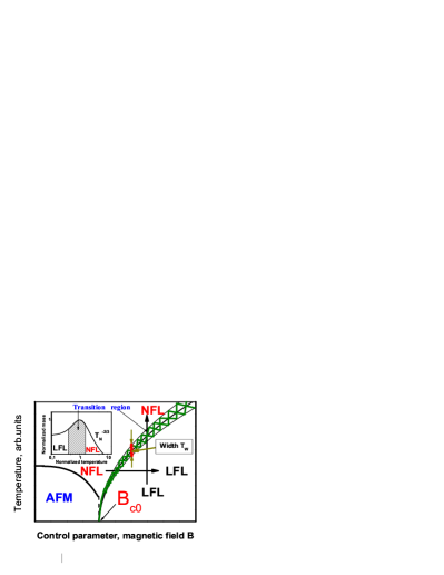
Рис. 11: Schematic phase diagram of $\rm YbRh_{2}Si_{2}$ based on Eq. (29) with magnetic field as the control parameter $B$. The vertical and horizontal arrows show LFL-NFL and NFL-LFL transitions at fixed $B$ and fixed $T$ correspondingly. At $B<B_{c0}$ the system is in antiferromagnetic (AFM) state. The width of the transition regime $T_{w}\propto T$ is shown by the segment confined by the two vertical arrows. Inset shows a schematic plot of the normalized effective mass versus the normalized temperature. Transition regime, where $M^{*}_{N}$ reaches its maximum value at $y=T/T_{M}=1$, is shown by the hatched area both in the main panel and in the inset.

We now are in position to construct the schematic phase diagram of the HF metal $\rm YbRh_{2}Si_{2}$ at $B\ll B^{*}$. The pase diagram is reported in Fig. 11. The magnetic field $B$ plays a role of the control parameter, driving the system towards its QCP. In our case this QCP is of FCQPT type. The FCQPT peculiarity occurs at $B=B_{c0}$, yielding new strongly degenerate state at $B<B_{c0}$. To lift this degeneracy, the system forms either superconducting (SC) or magnetically ordered (ferromagnetic (FM), antiferromagnetic (AFM) etc) states prep . In the case of $\rm YbRh_{2}Si_{2}$, this state is AFM one steg1 . As it follows from Eqs. (29) and (30) and seen from Fig. 11, at $B\geq B_{c0}$ the system is in either NFL or LFL states. At fixed temperatures the increase of $B$ drives the system along the horizontal arrow from NFL state to LFL one. On the contrary, at fixed magnetic field and raising temperatures the system transits along the vertical arrow from LFL state to NFL one. The inset to Fig. 11 demonstrates the behavior of the normalized effective mass $M^{*}_{N}=M^{*}/M^{*}_{M}$ versus normalized temperature $y=T/T_{M}$ following from Eq. (29). The $T^{-2/3}$ regime is marked as NFL one since (contrary to LFL case where the effective mass is constant) the effective mass depends strongly on temperature. It is seen that temperature region $y\sim 1$ signifies a transition regime between the LFL behavior with almost constant effective mass and NFL one, given by $T^{-2/3}$ dependence. Thus, temperatures $T\simeq T_{M}$, shown by arrows in the inset and main panel, can be regarded as a transition regime between LFL and NFL states. It is seen from Eq. (30) that the width of the transition regime $T_{w}\propto T$ is proportional to $(B-B_{c0})$. It is shown by the segment between two vertical arrows in Fig 11. These theoretical results are in good agreement with the experimental facts steg1 ; pnas .

In Fig. 12, our calculations of the normalized effective mass $M^{*}_{N}(T_{N})$ at fixed magnetic field $B^{*}$ making the system fully polarized are shown by the solid line. Figure 12 reveals the scaling behavior of the normalized experimental curves - the scaled curves at different magnetic fields $B$ merge into a single one in terms of the normalized variable $y=T/T_{M}$. It is seen from Fig. 12 that our calculations are in accord with facts steg1 : At elevated temperatures ($y\simeq 1$) the LFL state first changes into the transition regime and then disrupts into the NFL state.

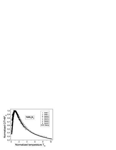
Рис. 12: The normalized effective mass $M^{*}_{N}=M^{*}/M^{*}_{M}$ versus normalized temperature $T_{N}=T/T_{M}$. $M^{*}_{N}$ is extracted from the data shown in Fig. 3. Magnetic fields $B$ is listed in the legend. Our calculations (made at $B\simeq B^{*}$ when the quasiparticle band is fully polarized) are depicted by the solid curve tracing the scaling behavior of $M^{*}_{N}$.

To get further insight into the behavior of the system at high magnetic fields, in Fig. 13 we collect the curves $M^{*}_{N}(T_{N})$ both at low (symbols in the upper box in Fig. 13) and high (symbols in the lower box) magnetic fields $B$. All curves have been extracted from the experimental facts steg1 ; oesb . It is seen that while at low fields the low-temperature ends ($T_{N}\sim 0.1$) of the curves completely merge, at high fields this is not the case. Moreover, the low-temperature asymptotic value of $C/T=M^{*}_{N}$ at low fields is around two times more then that at high fields. The physical reason for low-field curves merging is that the effective mass does not depend on spin variable so that the polarizations of subbands with $\sigma_{\uparrow}$ and $\sigma_{\downarrow}$ are almost equal to each other. This is reflected in our calculations, based on Eq. (29) for low magnetic fields $B<<B^{*}$. The result is shown by the dotted line in Fig. 13.

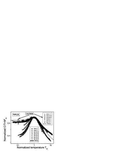
Рис. 13: Joint behavior of the normalized effective mass $M^{*}_{N}$ at low (upper box symbols) and high (lower box symbols) magnetic fields extracted from the specific heat ($C/T$) measurements of the $\rm YbRh_{2}Si_{2}$ oesb . Our low-field calculations are depicted by the dotted line tracing the scaling behavior of $M^{*}_{N}$. Our high-field calculations (solid line) are taken at $B\sim B^{*}$ when the quasiparticle band becomes fully polarized.

It is also seen from Fig. 13 that all low-temperature differences between high- and low field behavior of the normalized effective mass disappear at high temperatures. In other words, while at low temperatures the values of $M^{*}_{N}$ for low fields are two times more then those for high fields, at temperatures $T_{N}\geq 1$ this difference disappear. It is seen that these high temperatures lie about the transition region, marked by hatched area in the inset to Fig. 11. This means that two states (LFL and NFL) separated by the transition region are clearly seen in Fig. 13 displaying good agreement between our calculations (dotted line for low fields and thick line at high fields) and the experimental points (symbols).

Contrary to the low fields case, at high fields $B\sim B^{*}$ (symbols in the lower box of Fig. 13), in the low temperature LFL state the curves $M^{*}_{N}(T_{N})$ do not merge into single one and their values decrease as $B$ grows representing the full spin polarization of the HF band at the highest reached magnetic fields. As we have mentioned above, at temperature raising all effects of spin polarization smear down, yielding the restoration NFL behavior at $T\simeq\mu_{B}B$. Our high-field calculations (solid line in Fig. 13) reflect the latter fact and are also in good agreement with experimental facts. In order not to overload Fig. 13 with unnecessary details, we show the calculations only for the case of the full spin polarization.

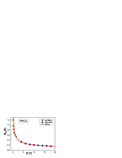
Рис. 14: The maxima $M^{*}_{M}(B)$ of the functions $C/T$ versus magnetic field $B$ for $\rm YbRh_{2}Si_{2}$. The maxima taken at the low fields oesb are shown by the solid squares, the ones taken at the high fields steg1 are depicted by the solid circles. The solid curve is approximated by $M^{*}_{M}(B)\propto d/\sqrt{B-B_{c0}}$, $d$ is a fitting parameter.

Figure 14 reports the maxima $M^{*}_{M}(B)$ of the functions $C/T$ shown in Fig. 3 versus $B$ depicted by the solid circles and the solid squares, corresponding measurements on $\rm YbRh_{2}Si_{2}$ taken at the low magnetic fields oesb . The solid line represents the approximation describing the maxima value of $M^{*}(B)\propto\sqrt{B-B_{c0}}$ calculated within the framework of FCQPT theory shag4 ; prep . It is seen that our calculations are in good agreement with the experimental facts over two decades in magnetic field $B$. The agreement indicates that at $T\simeq\mu_{B}B$ the transition regime takes place and the NFL behavior restores at higher temperatures $T\sim 20$ K.

In Fig. 15, the solid squares and circles denote temperatures $T_{N}(B)$ at which the maxima of $C/T$ take place. To fit the experimental data steg1 ; oesb the function $T_{N}(B)=b(B-B_{c0})$ defined by Eq. (30) is used. It is seen from Fig. 15 that our calculations shown by the solid line are in accord with experimental facts, and we conclude that the transition regime of $\rm YbRh_{2}Si_{2}$ is restored at temperatures $T\simeq\mu_{B}B$.

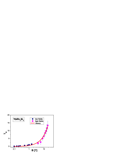
Рис. 15: The temperatures $T_{M}(B)$ at which the maxima of $C/T$ are located versus magnetic field $B$ for $\rm YbRh_{2}Si_{2}$. The solid squares denote $T_{M}$ taken in measurements at the low magnetic fields oesb . The solid circles denote $T_{M}$ at the high magnetic fields steg1 . The solid line represents the function $T_{M}\propto b(B-B_{c0})$, $b$ is a fitting parameter, see Eq. (30).

Consider now the magnetization $M(B,T)$ as a function of magnetic field $B$ at fixed temperature $T=T_{f}$

$$M(B,T)=\int_{0}^{B}\chi(z,T)dz,$$ (31)

where the magnetic susceptibility $\chi$ is given by landau ; lanl1

$$\chi(B,T)=\frac{\beta M^{*}(B,T)}{1+F_{0}^{a}}.$$ (32)

Here, $\beta$ is a constant and $F_{0}^{a}$ is the Landau amplitude related to the exchange interaction.

At low magnetic fields, $B\ll B^{*}$, our calculations show that the magnetization exhibits a kink at some magnetic field $B=B_{k}$. The experimental magnetization demonstrates the same behavior steg ; oesbs . We use $B_{k}$ and $M(B_{k})$ to normalize $B$ and $M$ respectively. Due to the normalization the coefficients $\beta$ and $(1+F_{0}^{a})$ drop out from the result, and $\chi\propto M^{*}$ prep . So we can use Eq. (28) to calculate the magnetic susceptibility $\chi$. The normalized magnetization $M(B)/M(B_{k})$ both extracted from experiment (symbols) and calculated one (solid line), are reported in the inset to Fig. 16. It shows that our calculations are in good agreement with the experimental facts, and all the data exhibit the kink (shown by the arrow) at $B_{N}\simeq 1$ taking place as soon as the system enters the transition region corresponding to the magnetic fields where the horizontal arrow in Fig. 11 crosses the hatched area. To illuminate the kink position, in the Fig. 16 we present the $M(B)$ dependence in logarithmic - logarithmic scale. In that case the straight lines show clearly the change of the power dependence $M(B)$ at the kink.

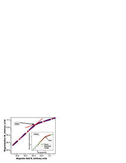
Рис. 16: The calculated magnetization $M(B)$ (symbols) and straight lines which are guides for eye. The intersection of the straight lines visualize the kink at the crossover region in the Fig. 11. The inset: The field dependencies of the normalized magnetization $M$ of $\rm{YbRu_{2}Si_{2}}$ oesbs at $T=0.05$ K. The kink (shown by the arrow) is clearly seen at the normalized field $B_{N}=B/B_{k}\simeq 1$. The solid curve represents our calculations.

At magnetic field $B\simeq B^{*}$ the quasiparticle band becomes fully polarized and a new kink appears steg1 ; mal , we call this kink as the second one. Our calculations of the normalized magnetization (line) and the experimental points (squares) are shown in Fig. 17. In that case both the magnetization and the field are normalized by the corresponding values at the second kink.

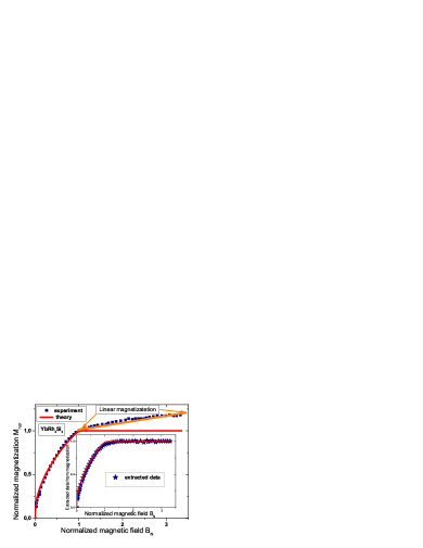
Рис. 17: The normalized magnetization $M_{nor}$ as a function of the normalized magnetic field $B_{N}$. The calculated magnetization is shown by the solid line, and the experimental facts steg1 is represented by the solid squares. The linear dependence of $M_{nor}$ on $B_{N}$ is shown by the arrows. The inset demonstrates the experimental data with the subtracted linear dependence depicted by the stars. Our calculations is shown by the solid line.

In the Fig. 17 we plot our calculated magnetization (in the variables $B$ and $M$ normalized to those in the second kink point) versus experimental one. The marvelous coincidence is seen everywhere except the high-field part at $B_{N}\geq 1$ where the normalized magnetization $M_{nor}$ exhibits a linear dependence on $B_{N}$ depicted by the two arrows, while the calculated magnetization is approximately constant at these $B_{N}$. Such a behavior is the intrinsic shortcoming of the HF liquid model that takes into account only heavy electrons and omit the other conduction electrons that contribute to the magnetization c1 ; c2 . Thus, we can consider the high-field (at $B_{N}>1$) part of the magnetization as the contribution which does not included in our theory. To separate this contribution from the experimental magnetization curve, we (numerically) differentiate it, then subtract constant part at $B_{N}>1$ and integrate back the resulting curve. The coincidence between our calculations depicted by the solid curve and processed experimental data shown by the stars is reported in the inset to Fig. 17. As we can see now, the coincidence between the theory and experiment is good in the entire magnetic field domain. Taking into account the obtained results displayed in Figs. 13—17, we conclude that the HF system of $\rm{YbRu_{2}Si_{2}}$ evolves continuously under the application of magnetic fields. This observation is in agreement with experimental observations prl .

7 Summary

We have shown that the physics of systems with heavy fermions is determined by the extended quasiparticle paradigm. In contrast to the paradigm that the quasiparticle effective mass is a constant, within the extended quasiparticle paradigm the effective mass of new quasiparticles strongly depends on the temperature, magnetic field, pressure, and other parameters. The quasiparticles are well defined and can be used to describe the scaling behavior of the thermodynamic HF metals in a wide range of both temperatures $T$ and magnetic fields $B$.

It was demonstrated that the phase diagram of systems located near the fermion condensation quantum phase transition are strongly influenced by control parameters such as chemical pressure, pressure, the number density or magnetic field. Analyzing the phase diagram of $\rm YbRh_{2}Si_{2}$, we have found that under the application of the chemical pressure (positive/negative) QCP is destroyed or converted into the quantum critical line, correspondingly.

We have analyzed the thermodynamic properties of $\rm YbRh_{2}Si_{2}$ in both the low and the high magnetic fields. Our calculations allow us to conclude that in magnetic field the HF system of $\rm YbRh_{2}Si_{2}$ evolves continuously without a metamagnetic transition and possible localization of heavy $4f$ electrons. At low temperatures and under the application of magnetic field the HF system demonstrates the LFL behavior, at elevated temperatures the system enters the transition region followed by the NFL behavior.

Our observations are in good agreement with experimental facts and show that the fermion condensation quantum phase transition is indeed responsible for the observed NFL behavior and quasiparticles survive both high temperatures and high magnetic fields.

- (1) A. B. Migdal, Theory of Finite Fermi Systems and Applications to Finite Nuclei (Interscience, London, 1967).
- (2) A. B. Migdal, Phys. Lett. B 45, 448 (1973).
- (3) V. A. Khodel and V. R. Shaginyan, Pis’ma Zh. Eksp. Teor. Fiz. 51, 488 (1990) [JETP Lett. 51, 553 (1990)].
- (4) V. A. Khodel, V. A. Shaginyan, and V. V. Khodel, Phys. Rep. 249, 1 (1994).
- (5) G. E. Volovik, Pis’ma Zh. Eksp. Teor. Fiz. 53, 208 (1991); [JETP Lett. 53, 222 (1991)].
- (6) G.E. Volovik, Springer Lecture Notes in Phys. 718, 31 (2007).
- (7) V. A. Khodel, J. W. Clark, H. Li, and M. V. Zverev, Phys. Rev. Lett. 98, 216404 (2007).
- (8) V. R. Shaginyan, M. Ya. Amusia, A. Z. Msezane, and K. G. Popov, Phys. Rep. 492, 31 (2010).
- (9) G. R. Stewart, Rev. Mod. Phys. 73, 797 (2001).
- (10) C. M. Varma, Z. Nussionov, and W. van Saarloos, Phys. Rep. 361, 267 (2002).
- (11) H. v. Löhneysen, A. Rosch, M. Vojta, and P. Wölfle, Rev. Mod. Phys. 79, 1015 (2007).
- (12) M. Vojta, Rep. Prog. Phys. 66, 2069 (2003).
- (13) V. R. Shaginyan, M. Ya. Amusia, and K. G. Popov, Usp. Fiz. Nauk 177, 586 (2007), [Phys. Usp. 50, 563 (2007)].
- (14) P. Coleman, Lectures on the Physics of Highly Correlated Electron Systems VI, in: American Institute of Physics, Ed. by F. Mancini (New York, 2002, 79).
- (15) L. D. Landau, Zh. Eksp. Teor. Fiz. 30, 1058 (1956); [Sov. Phys. JETP 3, 920 (1956)].
- (16) E. M. Lifshitz and L.P. Pitaevskii, Statisticheskaya Fizika (Statistical Physics), Part 2 (Nauka, Moscow, 1978; Translated into English, Pergamon Press, Oxford, 1980).
- (17) A. B. Migdal, Nuclear Theory: the Quasiparticle Method (Benjamin, 1968).
- (18) D. Pines and P. Noziéres, Theory of Quantum Liquids (Benjamin, New York, 1966).
- (19) P. Coleman and A. J. Schofield, Nature 433, 226 (2005).
- (20) P. Coleman, C. Pépin, Q. Si, and R. Ramazashvili, J. Phys. Condens. Matter 13, R723 (2001).
- (21) R. Küchler, N. Oeschler, P. Gegenwart et al., Phys. Rev. Lett. 91, 066405 (2003).
- (22) V. R. Shaginyan, J. G. Han, and J. Lee, Phys. Lett. A 329, 108 (2004).
- (23) V. A. Khodel, J. W. Clark, and M. V. Zverev, Phys. Rev. B 78, 075120 (2008).
- (24) V. A. Khodel, JETP Lett. 86, 721 (2007).
- (25) P. Coleman, Physica Status Solidi B 247, 506 (2010).
- (26) C. Proust, E. Boaknin, R. W. Hill et al., Phys. Rev. Lett. 89, 147003 (2002).
- (27) P. Gegenwart, J. Custers, C. Geibel et al., Phys. Rev. Lett. 89, 056402 (2002).
- (28) K. Kadowaki and S. B. Woods, Solid State Commun. 58, 507 (1986).
- (29) A. J. Millis, A. J. Schofield, G. G. Lonzarich, and S. A. Grigera, Phys. Rev. Lett. 88, 217204 (2002).
- (30) R. Bel, K. Behnia, Y. Nakajima et al., Phys. Rev. Lett. 92, 217002 (2004).
- (31) J. Paglione, M. A. Tanatar, D. G. Hawthorn et al., Phys. Rev. Lett. 91, 246405 (2003).
- (32) J. Paglione, M. A. Tanatar, D. G. Hawthorn et al., Phys. Rev. Lett. 97, 106606 (2006).
- (33) F. Ronning, R. W. Hill, M. Sutherland et al., Phys. Rev. Lett. 97, 067005 (2006).
- (34) F. Ronning, C. Capan, E. D. Bauer et al., Phys. Rev. B 73, 064519 (2006).
- (35) J. D. Koralek, J. F. Douglas, N. C. Plumb et al., Phys. Rev. Lett. 96, 017005 (2006).
- (36) S. Fujimori, A. Fujimori, K. Shimada et al., Phys. Rev. B 73, 224517 (2006).
- (37) N. Oeschler, S. Hartmann, A. P. Pikul et al., Physica B 403, 1254 (2008).
- (38) P. Gegenwart, Y. Tokiwa, T. Westerkamp et al., New J. Phys. 8, 171 (2006).
- (39) P. Gegenwart, T. Westerkamp, C. Krellner et al., Physica B 403, 1184 (2008).
- (40) M. Neumann, J. Nyéki, B. Cowan, and J. Saunders, Science 317, 1356 (2007).
- (41) V. R. Shaginyan, M. Ya. Amusia, and K. G. Popov, Phys. Lett. A 373, 2281 (2009).
- (42) V. R. Shaginyan, M. Ya. Amusia, K. G. Popov, and S. A. Artamonov, JETP Lett. 90, 47 (2009).
- (43) V. R. Shaginyan, A. Z. Msezane, K. G. Popov, and V. A. Stephanovich, Phys. Rev. Lett. 100, 096406 (2008).
- (44) I. Yu. Pomeranchuk, Zh. Eksp. Teor. Fiz. 35, 524 (1958); [Sov. Phys. JETP 8, 361 (1959)].
- (45) L. N. Oliveira, E. K. U. Gross, and W. Kohn, Phys. Rev. Lett. 60, 2430 (1988).
- (46) V. R. Shaginyan, Phys. Lett. A 249, 237 (1998).
- (47) M. Ya. Amusia and V. R. Shaginyan, Phys. Lett. A 269, 337 (2000).
- (48) V. R. Shaginyan, Pis’ma Zh. Eksp. Teor. Fiz. 68, 491 (1998); [JETP Lett. 68, 527 (1998)].
- (49) A. V. Chubukov, D. L. Maslov, and A. J. Millis, Phys. Rev. B 73, 045128 (2006).
- (50) D. Vollhardt, Rev. Mod. Phys. 56, 99 (1984).
- (51) M. Pfitzner and P. Wölfe, Phys. Rev. B 33, 2003 (1986).
- (52) D. Vollhardt, P. Wölfle, and P. W. Anderson, Phys. Rev. B 35, 6703 (1987).
- (53) V. M. Yakovenko and V. A. Khodel, JETP Lett. 78, 850 (2003).
- (54) V. R. Shaginyan, JETP Lett. 77, 104 (2003).
- (55) A. Casey, H. Patel, J. Nyeki et al., J. Low Temp. Phys. 113, 293 (1998).
- (56) A. A. Shashkin, S. V. Kravchenko, V. T. Dolgopolov, and T. M. Klapwijk, Phys. Rev. B 66, 073303 (2002).
- (57) A. A. Shashkin, M. Rahimi, S. Anissimova et al., Phys. Rev. Lett. 91, 046403 (2003).
- (58) J. Boronat, J. Casulleras, V. Grau et al., Phys. Rev. Lett. 91, 085302 (2003).
- (59) Y. Zhang, V. M. Yakovenko, and S. Das Sarma, Phys. Rev. B 71, 115105 (2005).
- (60) Y. Zhang and S. Das Sarma, Phys. Rev. B 70, 035104 (2004).
- (61) V. A. Khodel, V. R. Shaginyan, and M. V. Zverev, JETP Lett. 65, 242 (1997).
- (62) S. V. Kravchenko and M. P. Sarachik, Rep. Prog. Phys. 67, 1 (2004).
- (63) A. Casey, H. Patel, J. Cowan, and B. P. Saunders, Phys. Rev. Lett. 90, 115301 (2003).
- (64) V. A. Khodel, V. R. Shaginyan, and P. Shuk, Pis’ma Zh. Eksp. Teor. Fiz. 63, 719 (1996); [JETP Lett. 63, 752 (1996)].
- (65) M. Ya. Amusia and V. R. Shaginyan, Pis’ma Zh. Eksp. Teor. Fiz. 73, 268 (2001); [JETP Lett. 73, 232 (2001)].
- (66) M. Ya. Amusia and V. R. Shaginyan, Phys. Rev. B 63, 224507 (2001).
- (67) V. R. Shaginyan, Physica B 312-313C, 413 (2002).
- (68) G. E. Volovik, Acta Phys. Slov. 56, 49 (2006).
- (69) J. Bardeen, L. N. Cooper, and J. R. Schrieffer, Phys. Rev. 108, 1175 (1957).
- (70) V. A. Khodel, M. V. Zverev, and V. M. Yakovenko, Phys. Rev. Lett. 95, 236402 (2005).
- (71) S. Friedemann, T. Westerkamp, M. Brando et al., Nat. Phys. 5, 465 (2009).
- (72) J. Custers, P. Gegenwart, C. Geibel et al., Phys. Rev. Lett. 104, 186402 (2010).
- (73) Y. Tokiwa, P. Gegenwart, C. Geibel, and F. Steglich, J. Phys. Soc. Jpn. 78, 123708 (2009).
- (74) V. R. Shaginyan, K. G. Popov, V. A. Stephanovich et al., Europhys. Lett. 93, 17008 (2011).
- (75) J. W. Clark, V. A. Khodel, and M. V. Zverev, Phys. Rev. B 71, 012401 (2005).
- (76) D. Takahashi, S. Abe, H. Mizuno et al., Phys. Rev. B 67, 180407(R) (2003).
- (77) S. Friedemann, N. Oeschler, S. Wirth, et al., Proc. Natl. Acad. Sci. USA 107, 14547 (2010).
- (78) V. R. Shaginyan, Pis’ma Zh. Eksp. Teor. Fiz. 79, 344 (2004); [JETP Lett. 79, 286 (2004)].
- (79) P. Gegenwart, T. Westerkamp, C. Krellner et al., Science 315, 969 (2007).
- (80) S. V. Kusminskiy, K. S. D. Beach, A. H. Castro Neto, and D. K. Campbell, Phys. Rev. B 77, 094419 (2008).
- (81) T. Saso and M. Itoh, Phys. Rev. B 53, 6877 (1996).
- (82) H. Satoh and F. J. Ohkawa, Phys. Rev. B 63, 184401 (2001).
- (83) P. M. C. Rourke, A. McCollam, G. Lapertot et al., Phys. Rev. Lett. 101, 237205 (2008).