Josephson and Andreev transport through quantum dots

Abstract

In this article we review the state of the art on the transport properties of quantum dot systems connected to superconducting and normal electrodes. The review is mainly focused on the theoretical achievements although a summary of the most relevant experimental results is also given. A large part of the discussion is devoted to the single level Anderson type models generalized to include superconductivity in the leads, which already contains most of the interesting physical phenomena. Particular attention is paid to the competition between pairing and Kondo correlations, the emergence of $\pi$-junction behavior, the interplay of Andreev and resonant tunneling, and the important role of Andreev bound states which characterized the spectral properties of most of these systems. We give technical details on the several different analytical and numerical methods which have been developed for describing these properties. We further discuss the recent theoretical efforts devoted to extend this analysis to more complex situations like multidot, multilevel or multiterminal configurations in which novel phenomena is expected to emerge. These include control of the localized spin states by a Josephson current and also the possibility of creating entangled electron pairs by means of non-local Andreev processes.

I Introduction

The field of electronic transport in nanoscale devices is experiencing a fast evolution driven both by advances in fabrication techniques and by the interest in potential applications like spintronics or quantum information processing. Within this context quantum dot (QD) systems are playing a central role. These devices have several different physical realizations including semiconducting heterostructures, small metallic particles, carbon nanotubes or other molecules connected to metallic electrodes. In spite of this variety a very attractive feature of these devices is that they can usually be described theoretically by simple ”universal-like” models characterized by a few parameters. In addition to their potential applications, these systems provide a unique test-bed for analyzing the interplay of electronic correlations and transport properties in nonequilibrium conditions.

Electron transport in semiconducting QDs has been studied since the early 90’s when phenomena like Coulomb blockade (CB) was first observed Kastner (1993). It soon became clear that QDs could allow to study the effect in transport properties of basic electronic correlations phenomena like the Kondo effect as suggested in early predictions Glazman and Raikh (1988); Lee and Ng (1988). These predictions were first tested in metallic nanoscale junctions containing magnetic impurities Ralph and Burhman (1994). However, a definitive breakthrough in the field came with the observation of this effect in semiconducting QDs by Goldhaber et al. Goldhaber-Gordon et al. (1998) and Cronenwett et al. Cronenwett et al. (1998). A great advantage of these devices is to offer the possibility of controlling the relevant parameters, thus allowing a more direct comparison with the theoretical predictions. Since then the effect of Kondo correlations in electronic transport has been observed in several physical realizations of QDs based on carbon nanotubes (CNTs) Nygard et al. (2000) and big molecules like fullerenes Roch et al. (2009).

In parallel to these advances the study of superconducting (SC) transport in nanoscale devices has also experienced a great development. From a theoretical point of view, with the advent of mesoscopic physics, a more detailed understanding of superconducting transport was developed around the central concept of coherent Andreev reflection (AR) Andreev (1964); Beenakker (1997). This concept has allowed to unify the description of superconducting transport in different types of structures like normal metal-superconductor (N-S), S-N-S junctions and superconducting quantum point contacts (SQPC). Due to the multiple AR (MAR) mechanism the spectral density of systems like S-N-S or SQPCs is characterized by the presence of the so-called Andreev bound states (ABS) inside the superconducting gap. These states are sensitive to the superconducting phase difference and are thus current-carrying states which usually give the dominating contribution to the Josephson effect.

In recent years it has become feasible to produce hybrid systems combining different physical realizations of QDs well contacted to superconducting electrodes (for a review see Franceschi et al. (2010)). Superconducting transport through QDs provides the interesting possibility to explore the interplay of the AR mechanism and typical QD phenomena like CB and Kondo effect. The central aim of this review article is to discuss the main advances which have taken place on this issue during the last years.

A usual assumption in these studies is that a basic description of the main properties of these hybrid systems can be provided by the Anderson model and its generalizations to include SC leads, orbital degeneracy, etc. The single level model applies when the dot level spacing $\delta\epsilon$ is larger than all other relevant energy scales. In the normal state the model allows to describe in a unified way CB and the Kondo effect both in and out of equilibrium conditions Kouwenhoven and Glazman (2001). With two superconducting leads interesting new physics already appear in the equilibrium case. Due to the Josephson effect, electron transport is possible without an applied bias voltage and the model describes the competition between Kondo effect and induced pairing within the dot. Figure 1 illustrates this competition: depending on the ratio between the Kondo temperature, $T_{K}$, and the superconducting order parameter, $\Delta$, there is a phase transition between a Kondo dominated spin-singlet ground state to a degenerate magnetic ground state. This transition is accompanied by a reversal of the sign of the Josephson current. Thus in the magnetic case the S-QD-S system constitutes a realization of the so-called $\pi$-junction Glazman and Matveev (1989); Spivak and Kivelson (1964). A more detailed understanding of this transition describing the appearance of intermediate phases with metastable states was achieved more recently Rozhkov and Arovas (1999); Vecino et al. (2003). The realization of a $\pi$-junction in QD systems should distinguished from the similar phenomena in SFS junctions, where F denotes a ferromagnetic material Golubov et al. (2004).

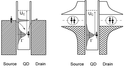
Figure 1: Schematic representation of a single spin-degenerate level QD connected to normal (left panel) and superconducting (right panel) leads with a large charging energy $U_{c}$. In the normal case the local density of states (LDOS) in the dot exhibits the typical form corresponding to the Kondo regime with a narrow resonance at the Fermi energy and a a broad resonance (of width $\Gamma$) below it. In the superconducting case the Kondo resonance (assumed to be narrower than the superconducting gap) disappears due to the competition with the pairing correlations in the leads. Courtesy of C. Schönenberger.

Another basic situation which has been extensively explored (both theoretically and experimentally) is the N-QD-S case. This situation has been mainly analyzed in the linear transport regime in which it exhibits and interesting interplay between Kondo behavior and resonant Andreev reflection. In contrast to the S-QD-S case this system does not exhibit a quantum phase transition but there is instead a crossover from a Kondo dominated regime for large $T_{K}/\Delta$ to a singlet superconducting regime in the opposite limit.

A third paradigmatic situation which has been studied is the voltage biased S-QD-S system. This situation constitutes a much more demanding task for the theory due to the need of describing properly the strong out-of-equilibrium distribution which is generated by the infinite series of multiple Andreev reflection (MAR) processes together with the effects of Coulomb interactions. The problem becomes simpler in two limiting cases: 1) when Coulomb interactions are small and treated in a mean field approximation thus allowing to analyze the interplay of MAR and resonant tunneling and 2) when the Coulomb energy is the larger energy scale in the problem and the contribution of MAR processes are largely suppressed.

More recent developments include the study of several QDs (connected either in series or in parallel) coupled to one or more SC electrodes. In these situations there is a competition between not only the Kondo and the SC correlations but also the possible magnetic coupling of the spins localized within the dots. This could open the possibility to control the spin state of the dots system by means of the Josephson current.

In addition there is a growing interest in analyzing transport in these hybrid structures in a multiterminal configuration. One of the aims of these studies is the detection and control of non-local Andreev processes, which offer the possibility of producing entangled electron pairs Recher et al. (2001).

This review article is organized as follows: in Section II we introduce the basic theoretical models used to describe the hybrid QD systems, which are largely based on the Anderson model and its generalizations. In this section we also give a brief summary of the application of nonequilibrium Green functions techniques for the calculation of the electronic properties within these type of models. Section III is devoted to review the main results for the S-QD-S systems in equilibrium, i.e. in the dc Josephson regime. We first discuss the case of a non-interacting resonant level which is useful to illustrate the emergence of ABSs and its contribution to the Josephson current. In the subsequent subsections we give account of the different theoretical methods which have been used to analyze the effect of interactions in the dc Josephson regime. A main issue which is discussed in this section are the phase diagrams describing the transition to the $\pi$-state as a function of the model parameters. We also give a brief account of the existing experimental results for S-QD-S devices in this regime. The case of a QD coupled to both a normal and a superconducting leads (N-QD-S) is addressed in Section IV. Most of the results obtained for this systems correspond to the linear regime with different levels of approximation to include the Coulomb interactions. We also briefly mention existing results for the non-linear regime and the few experiments which have been reported of this case up to date. Section V is devoted to the voltage biased S-QD-S system. We first give some technical details on the calculations for the non-interacting case in order to illustrate how to deal with the out of equilibrium MAR mechanism. We also comment in this section the few existing results including interactions in this regime and give an account of the related experiments. Finally, in Section VI we discuss several different situations which go beyond the single-level two-terminal case discussed in the previous sections. These include: multidot systems connected either in parallel or in series, the multilevel situation and setups in a multiterminal configuration. We conclude this article with a brief discussion of related issues not included in the present review and of topics which, in our view, deserve to be further analyzed in the near future.

II Basic models and formalism

The minimal model for a QD coupled to metallic electrodes in the regime where $\delta\epsilon$ is sufficiently large to restrict the analysis to a single spin-degenerate level is provided by the single level Anderson model Anderson (1961), with the Hamiltonian $H=H_{L}+H_{R}+H_{T}+H_{QD}$ where $H_{QD}$ corresponds to the uncoupled dot given by

$$H_{QD}=\sum_{\sigma}\epsilon_{0}c^{\dagger}_{0\sigma}c_{0\sigma}+Un_{0\uparrow}n_{0\downarrow},$$ (1)

where $c^{\dagger}_{0\sigma}$ creates and electron with spin $\sigma$ on the dot level located at $\epsilon_{0}$ and $U$ is the local Coulomb interaction for two electrons with opposite spin within the dot ($n_{0\sigma}=c^{\dagger}_{0\sigma}c_{0\sigma}$). On the other hand, $H_{L,R}$ describe the uncoupled left and right leads which can be either normal or superconducting. In this last more general case, they are usually represented by a BCS Hamiltonian of the type

$$H_{\nu}=\sum_{k\sigma}\xi_{k,\nu}c^{\dagger}_{k\sigma,\nu}c_{k\sigma,\nu}+\sum_{k}\left(\Delta_{\nu}c^{\dagger}_{k\uparrow,\nu}c^{\dagger}_{-k\downarrow,\nu}+\mbox{h.c.}\right),$$ (2)

where $c^{\dagger}_{k\sigma,\nu}$ creates an electron with spin $\sigma$ at the single-particle energy level $\xi_{k,\nu}$ of the lead $\nu=L,R$ (usually referred to the lead chemical potential, i.e. $\xi_{k,\nu}=\epsilon_{k,\nu}-\mu_{\nu}$) and $\Delta_{\nu}=|\Delta_{\nu}|\exp{(i\phi_{\nu})}$ is the (complex) superconducting order parameter on lead $\nu$. Finally, $H_{T}$ describes the coupling between the QD level to the leads and has the form

$$H_{T}=\sum_{k\sigma,\nu}\left(V_{k,\nu}c^{\dagger}_{k\sigma,\nu}c_{0\sigma}+\mbox{h.c.}\right).$$ (3)

In order to reduce the number of parameters it is usually assumed that the normal density of states of the leads $\rho_{\nu}(\omega)$ is a constant in the range of energies around the Fermi level of the order of the superconducting gap and that the $k$ dependence of the hopping elements $V_{k\nu}\simeq V_{\nu}$ can be neglected within this range. The coupling to the leads is then characterized by a single parameter $\Gamma_{\nu}=\pi\rho_{\nu}|V_{\nu}|^{2}$, which can be interpreted as the normal tunneling rate from the dot to the leads.

Within the above model $\Delta_{\nu}=0$ would correspond to the normal state. For vanishing $\Gamma_{\nu}$ the model is in the so-called atomic limit which is characterized by sharp peaks in the spectral density at $\epsilon_{0}$ and $\epsilon_{0}+U$. This limit corresponds to the Coulomb blockade regime in an actual QD where the conductance is strongly suppressed except at the charge degeneracy points. When the couplings to the leads increase ($\Gamma_{\nu}$ become larger than temperature) virtual processes allow the charge and spin in the dot to fluctuate and a resonance at around the Fermi energy appears close to half-filling due to the Kondo effect. This simple model thus already captures the most relevant Physics of ultrasmall QDs with well separated energy levels, like the crossover from the Coulomb blockade to the Kondo regime as the temperature is lowered.

The simplicity of this model has allowed to obtain exact results in the equilibrium case by means of the Bethe ansatz Wiegmann and Tsvelick (1983). The most basic of these results is the expression for the Kondo temperature Hewson (1993)

$$T_{K}=\sqrt{\frac{U\Gamma}{2}}\exp{\left(-\frac{\pi|\epsilon_{0}(\epsilon_{0}+U)|}{2U\Gamma}\right)},$$ (4)

where $\Gamma=\Gamma_{L}+\Gamma_{R}$.

This temperature characterizes the crossover from the so-called local moment regime for $T\gg T_{K}$ to the regime where Kondo correlations between the localized spin within the QD and the spin of the electrons in the leads sets in. Although this physics is basically well understood since the 70’s for the case of magnetic impurities in metals, its consequences for transport in artificial nanostructures has started to be developed much more recently specially driven by the advances in fabrication techniques. In this respect while the linear transport properties are well understood still open questions remain regarding the non-equilibrium regime.

In the superconducting case another energy scale, associated with the superconducting gap, appears bringing additional complexity to the problem, whose description is in fact the scope of this review. Even in the equilibrium situation the Anderson model with superconducting leads contains the non-trivial Physics associated to the Josephson effect. A relevant parameter is then provided by the superconducting phase difference $\phi=\phi_{L}-\phi_{R}$.

In order to analyze the electronic and transport properties of a general superconducting system in the presence of interactions and in a non-equilibrium situation it is convenient to use Green function techniques. The Keldysh formalism provides the basic tools for this purpose.

Due to the presence of superconducting correlations it is convenient to introduce the Nambu spinor field operators $\Psi_{j},\Psi^{\dagger}_{j}$, with $\Psi^{\dagger}_{j}=\left(c^{\dagger}_{j\uparrow},c_{j\downarrow}\right)$ where $j=k\nu,0$ denotes the $\nu=L,R$ electrodes and the dot level respectively. The different terms in the model Hamiltonian of Eqs. (1), (2) and (3) can then be written as

$$H_{QD} = \Psi_{0}^{\dagger}\hat{h}_{0}\Psi_{0}+Un_{0\uparrow}n_{0\downarrow}$$

$$H_{\nu} = \sum_{k}\Psi_{k\nu}^{\dagger}\hat{h}_{k\nu}\Psi_{k\nu}$$

$$H_{T} = \sum_{k,\nu}\left(\Psi_{k\nu}^{\dagger}\hat{V}_{k\nu}\Psi_{0}+\mbox{h.c.}\right)\;\;,$$ (5)

where $\hat{h}_{0}=\epsilon_{0}\tau_{3}$, $n_{0\sigma}=\frac{1}{2}\Psi^{\dagger}_{0}\left[\tau_{0}+\mbox{sign}(\sigma)\tau_{3}\right]\Psi_{0}$, $\hat{h}_{k\nu}=\xi_{k\nu}\tau_{3}+\mbox{Re}{\Delta_{\nu}}\tau_{1}+\mbox{Im}{\Delta_{\nu}}\tau_{2}$, $\tau_{i=0,1,2,3}$ being the Pauli matrices defined in Nambu space.

Starting from these spinor field operators, generalized single-particle propagators can be defined along the Keldysh closed time loop as

$$\hat{G}^{\alpha\beta}_{j,j^{\prime}}(t,t^{\prime})=-i\langle T_{c}\left[\Psi_{j}(t_{\alpha})\Psi^{\dagger}_{j^{\prime}}(t^{\prime}_{\beta})\right]\rangle\;\;,$$ (6)

where $\alpha,\beta\equiv\pm$ denote the two branches in the Keldysh contour. These propagators allow to calculate in a straightforward way most of the relevant quantities like the mean charge and the superconducting order parameter within the dot as well as the mean current through it, which are given by

$$n_{0}(t) = i\mbox{Tr}\left(\tau_{3}\hat{G}^{+-}_{00}(t,t)\right)-1$$ (7)

$$\mbox{Re}{\Delta_{0}}(t) = U\mbox{Tr}\left(\tau_{1}\hat{G}^{+-}_{00}(t,t)\right)$$

$$I_{\nu}(t) = \frac{e}{\hbar}\sum_{k}\mbox{Tr}\left(\tau_{3}\left[\hat{V}_{k\nu}\hat{G}^{+-}_{k\nu,0}(t,t)-\hat{V}_{\nu k}\hat{G}^{+-}_{\nu k,0}(t,t)\right]\right).$$

These expressions are formally exact but of little use unless the single-particle propagators are known. Fully analytical and exact results can only be obtained in the non-interacting case. In the presence of interactions numerical methods allow to obtain exact results in the equilibrium case. In a more general case one is bound to find reasonable approximations for these propagators valid for a restricted range of parameters. It is usually convenient to express these approximations in terms of a self-energy $\Sigma$ which is related to the propagators by the usual Dyson equation

$$\breve{\hat{G}}_{00}=\breve{\hat{G}}^{(0)}_{00}+\breve{\hat{G}}^{(0)}_{00}\breve{\hat{\Sigma}}_{00}\breve{\hat{G}}_{00},$$ (8)

where $\breve{\hat{G}}^{(0)}$ denotes the unperturbed propagators corresponding to an appropriately defined non-interacting Hamiltonian $H_{0}$ (the $\breve{}$ symbol indicates matrix structure in Keldysh space) and where integration over internal times is implicitly assumed. Different approximations for the self-energy associated with electron-electron interactions are discussed in the forthcoming sections. The analysis of the problem is greatly simplified in the stationary case where Fourier methods can be applied both in the equilibrium and in the non-equilibrium situation. We shall start discussing in the next section the simplest possible case of an equilibrium situation. In this case further simplification arises from the possibility of expressing all Keldysh propagators in terms of the retarded-advanced propagators and the Fermi equilibrium distribution function, $n_{F}(\omega)=1/\left[1+\exp{\beta(\omega-\mu)}\right]$, where $\mu$ is the chemical potential and $\beta=1/k_{B}T$ as

$$\hat{G}^{+-}(\omega)=n_{F}(\omega)\left[G^{a}(\omega)-G^{r}(\omega)\right]\;\;.$$ (9)

Thus, for instance, the mean current can be written as

$$I_{\nu}=\frac{e}{h}\sum_{k}\int d\omega n_{F}(\omega)\mbox{Tr}\left[V_{k\nu}\mbox{Re}\left(G^{a}_{k\nu,0}-G^{r}_{k\nu,0}\right)\right].$$ (10)

III Equilibrium properties of quantum dots with superconducting leads

For a nanoscale system coupled to superconducting electrodes a finite current can flow even in the absence of an applied bias voltage due to the Josephson effect. We shall illustrate this effect starting from the non-interacting situation $(U=0)$ within the single level Anderson model introduced above. In this case the advanced-retarded Green function of the coupled dot can be expressed as

$$G^{a,r}_{00}(\omega)=\left(\begin{array}[]{cc}\omega-\epsilon_{0}-\Gamma_{L}g^{a,r}_{L}-\Gamma_{R}g^{a,r}_{R}&\Gamma_{L}e^{i\phi_{L}}f^{a,r}_{L}+\Gamma_{R}e^{i\phi_{R}}f^{a,r}_{R}\\ \Gamma_{L}e^{-i\phi_{L}}f^{a,r}_{L}+\Gamma_{R}e^{-i\phi_{R}}f^{a,r}_{R}&\omega+\epsilon_{0}-\Gamma_{L}g^{a,r}_{L}-\Gamma_{R}g^{a,r}_{R}\end{array}\right)^{-1},$$ (11)

where $f^{a,r}_{L,R}=|\Delta_{L,R}|/\sqrt{|\Delta_{L,R}|^{2}-(\omega\pm i0^{+})^{2}}$ and $g^{a,r}_{L,R}=-(\omega\pm i0^{+})f^{a,r}/|\Delta_{L,R}|$ are the dimensionless BCS green functions of the uncoupled leads. For simplicity we focus below on the case where both leads are of the same material for which $|\Delta_{L}|=|\Delta_{R}|=\Delta$.

The spectral density associated with this model exhibits bound states within the superconducting gap (i.e $|\omega|\leq\Delta$). Physically, the ABSs arise from virtual multiple Andreev reflection processes at the interface between the dot and each of the leads. In such processes and for energies inside the gap, the electrons (holes) incident towards the leads are reflected back as holes (electrons), as illustrated in Fig. 2. The condition for the appearance of ABSs is that the accumulated phase in the closed trajectory be a multiple of $2\pi$, which is equivalent to satisfying the equation

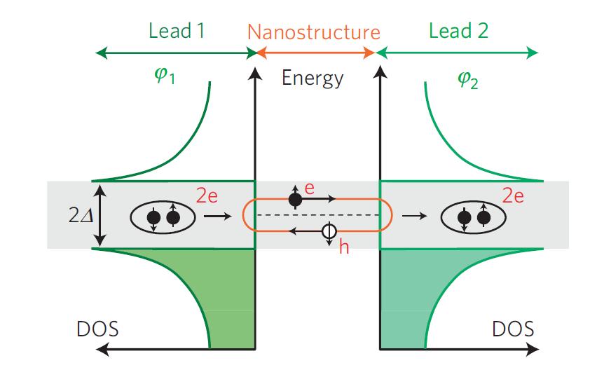
Figure 2: Schematic representation of the physical mechanism responsible for the formation of ABs in a generic nanostructure coupled to superconducting leads. Reprinted by permission from Macmillan Publishers Ltd: Nature Physics Pillet et al. (2010), copyright (2010).

$$D(\omega) \equiv \left[\omega-\epsilon_{0}-\Gamma g(\omega)\right]\left[\omega+\epsilon_{0}-\Gamma g(\omega)\right]$$ (12)

$$-|\Gamma_{L}e^{i\phi_{L}}+\Gamma_{R}e^{i\phi_{R}}|^{2}f(\omega)^{2}=0\;\;,$$

where we have used that the dimensionless BCS Green functions $g,f$ become real for energies inside the superconducting gap. It can be shown Rozhkov and Arovas (2000) that this equation has two real roots inside the gap $\pm\omega_{s}$, i.e. symmetrically located with respect to the Fermi energy.

An essential property of the ABSs is that they correspond to current-carrying states. In fact, due to its dependence on the superconducting phase difference they have associated a Josephson current $i_{s}(\phi)=2e/\hbar\left(\partial\omega_{s}/\partial\phi\right)$. The total Josephson current is obtained by adding the contribution of all states with finite occupation. Thus, at zero temperature only the lower ABS contributes and there is an additional contribution from the continuous spectrum $\omega<-\Delta$ which we discuss below.

The ABS equation (12) becomes particularly simple for an electron-hole and left-right symmetric case (i.e. $\epsilon_{0}=0$ and $\Gamma_{L}=\Gamma_{R}$) when it can be reduced to

$$\omega\pm\Delta\cos{\phi/2}+\frac{\omega\sqrt{\Delta^{2}-\omega^{2}}}{\Gamma}=0,$$ (13)

which for $\Gamma\gg\Delta$ has the simple solutions $\omega_{s}\simeq\pm\tilde{\Delta}\cos{\phi/2}$, where $\tilde{\Delta}$ is a reduced gap parameter which for $|\phi|\ll 1$ is given by $\tilde{\Delta}=\Delta\left[1-2(\Delta/\Gamma)^{2}\right]$. The ABSs for this case tend to the ones of a perfectly transmitting one channel superconducting contact $\pm\Delta\cos{\phi/2}$, the main qualitative difference being the reduced amplitude of their dispersion detaching them from the gap edges at $\phi=2n\pi$. This is illustrated in Fig. 3(a).

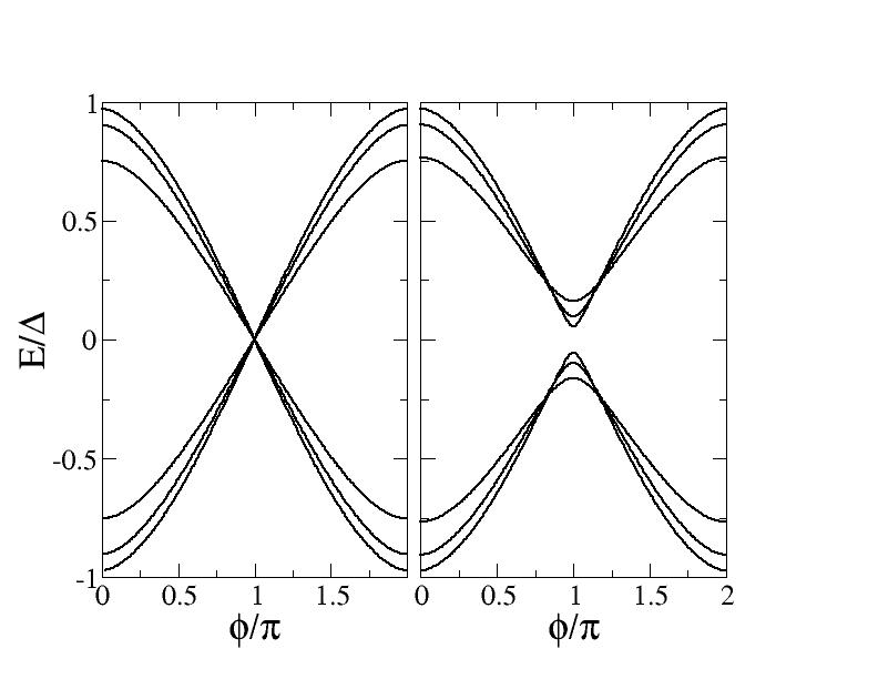
Figure 3: Andreev bound states for a non-interacting S-QD-S with different $\Gamma/\Delta$ values: 1.0, 2.0 and 4.0. Left panel corresponds to the e-h symmetric case ($\epsilon_{0}=0$) and the right panel to a case with $\epsilon_{0}=0.5\Delta$.

In the absence of electron-hole symmetry (i.e. $\epsilon_{0}\neq 0$) a finite internal gap between the upper and lower ABSs appears as in the case of a non-perfect transmitting one channel contact. When $\Delta/\Gamma\rightarrow 0$ the ABSs for this case are given by $\omega_{s}=\pm\Delta\sqrt{1-\tau\sin^{2}{(\phi/2)}}$, where $\tau=1/(1+(\epsilon_{0}/\Gamma)^{2})$ is the normal transmission at the Fermi energy. Outside this limiting case the ABSs exhibit both the internal gap and the detachment from the continuum states at $\phi=2n\pi$, as it is illustrated in Fig. 3(b).

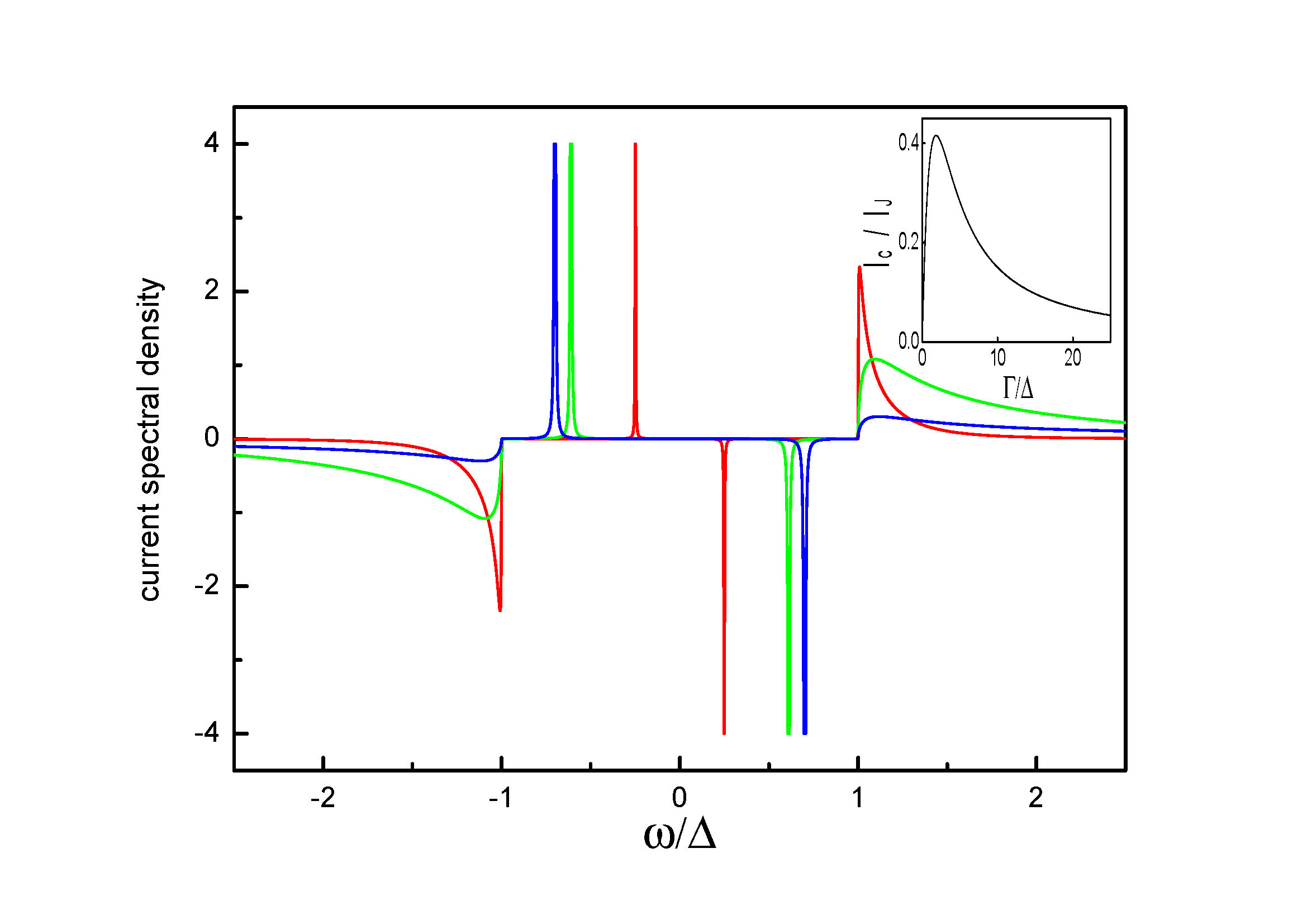
Figure 4: Current spectral density for the non-interacting S-QD-S system with $\epsilon_{0}$ and $\phi=1.5$ for increasing values of $\Gamma/\Delta=$ 0.5 (red), 4 (green) and 16 (blue). A small broadening has been introduced to help visualizing the ABs contribution, which has been truncated for the sake of clarity. The inset shows the relative contribution of the continuous spectrum $I_{c}$ compared to the total value $I_{J}$.

An interesting issue to comment is that the contribution from the states in the continuous spectrum becomes negligible when $\Delta/\Gamma\rightarrow 0$. In this limit the zero temperature current-phase relation (CPR) is simply given by

$$i_{s}(\phi)=\frac{e\Delta}{2\hbar}\frac{\tau\sin{\phi}}{\sqrt{1-\tau\sin^{2}{(\phi/2)}}}\;\;,$$ (14)

which is the CPR of a one channel contact with transmission $\tau$. For finite $\Delta/\Gamma$ there is a contribution from the continuum states. The expression for the total Josephson current in the non-interacting case can be derived from Eq. (10), which yields the following compact form

$$I=\frac{8e}{h}\Gamma_{L}\Gamma_{R}\sin{\phi}\int d\omega n_{F}(\omega)\mbox{Im}\left(\frac{f^{r}_{L}f^{r}_{R}}{D^{r}}\right).$$ (15)

The current density in Eq. (15) contains both the contribution from the ABSs (region $|\omega|<\Delta$) and from the continuous spectrum $|\omega|>\Delta$. The behavior of the current density as a function of $\Delta/\Gamma$ is depicted in Fig. 4. As can be observed the contribution from the continuous spectrum has the opposite sign compared to the one arising from the ABS. The inset shows that this contribution becomes negligible in the limit $\Delta/\Gamma\rightarrow 0$ and reaches a maximum for $\Delta/\Gamma\sim 2$.

In the rest of this section we shall discuss the different theoretical approaches to include the effect of interactions in the dc Josephson effect through single level QD models. We also include a subsection on experimental results.

III.1 Cotunneling approach

From a theoretical point of view the simplest approach to account for the effect of interactions in the Josephson current is to perform a perturbative expansion to the lowest non-zero order in the tunnel Hamiltonian. This so-called cotunneling approach was first used by Glazman and Matveev Glazman and Matveev (1989), who predicted the onset of the $\pi$-junction behavior by this method. More precisely they obtained for the $U\rightarrow\infty$ limit

$$I(\phi)=\lambda\frac{e}{\hbar}\frac{\Gamma_{L}\Gamma_{R}}{\Delta}F\left(\frac{|\epsilon_{0}|}{\Delta}\right)\sin\phi,$$ (16)

where $\lambda$ changes its value from 2 ($\epsilon_{0}>0$) to -1 ($\epsilon_{0}<0$), thus describing the transition to the $\pi$-phase, the function $F(x)$ having the form

$$F(x)=\frac{1}{\pi^{2}}\int\frac{dt_{1}dt_{2}}{(\cosh t_{1}+\cosh t_{2})(x+\cosh t_{1})(x+\cosh t_{2})}.\\$$

This approximation is clearly not valid for describing the Kondo regime ($T_{K}\gg\Delta$) which requires non-perturbative approaches like the ones discussed in following subsections.

III.2 Mean field and variational methods

Another simple approximate methods to deal with interactions are those of a mean field type like the Hartree-Fock approximation (HFA) or the slave-boson mean field (SBMF). In spite of their simplicity these approximations are able to capture important qualitative features due to interactions in certain limits.

We start by analyzing the HFA. In the context of magnetic impurities in superconductors this method was first applied by Shiba Shiba (1973), while for the analysis of the Josephson effect it was first considered in Ref. Rozhkov and Arovas (1999) and further analyzed in Vecino et al. (2003). Within this approximation electrons with a given spin “feel” a static potential due to the average occupation of the opposite spin, which corresponds to a simple constant self-energy $(\Sigma_{00})_{11}=U<n_{0\downarrow}>$ and $(\Sigma_{00})_{22}=-U<n_{0\uparrow}>$. In principle within the same level of approximation there appears a non-diagonal self-energy taking into account the induced pairing within the dot due to proximity effect, which can be written as $(\Sigma_{00})_{12}=U<c^{\dagger}_{0\uparrow}c^{\dagger}_{0\downarrow}>$. The effect of this non-diagonal contribution, which was not included in Ref. Rozhkov and Arovas (1999), was analyzed in Ref. Vecino et al. (2003). The determination of the self-energy in the HFA requires a self-consistent calculation by using Eqs. (II) which cannot be performed analytically in general.

The most significant result within the HFA is the appearance of a broken symmetry state in which the dot acquires a finite magnetic moment (i.e. $<n_{0\uparrow}>\neq<n_{0\downarrow}>$) for certain ranges of parameters. In this respect one should be cautious in principle as the HFA is known to predict also broken symmetry states for the same model with normal leads Anderson (1961), which are known to be spurious. However, for the superconducting case ground states with a finite magnetization do exist for certain parameter range as commented in the introduction. As it is shown below the HFA gives a rather good estimate of the magnetic ground state energy in the regions where it is the most stable phase.

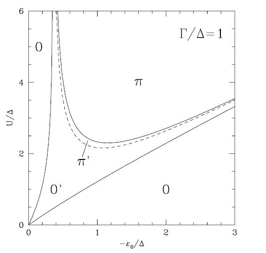
Figure 5: Phase diagram in the $U,-\epsilon_{0}$ plane for $\Gamma/\Delta=1$ obtained using the HFA Rozhkov and Arovas (1999)). The phases are classified into $0$, $0^{\prime}$, $\pi^{\prime}$ and $\pi$ as explained in the text. Reprinted figure with permission from A.V. Rozhkov and D. Arovas, Physical Review Letters 82, 2788, 1999 Rozhkov and Arovas (1999). Copyright (1999) by the American Physical Society.

The general properties of the ground state within the HFA are most conveniently displayed by a phase-diagram like the one in Fig. 5. In this diagram the notation ”0”, ”$0^{\prime}$”, ”$\pi^{\prime}$” and ”$\pi$” corresponds to the different ground state symmetries. Thus, ”0” corresponds to the non-magnetic case for all values of $\phi$ (the absolute energy minimum being located at $\phi=0$), while the ”$\pi$” denotes that the magnetic solution is the most stable for all $\phi$ values (with the absolute minimum at $\phi=\pi$). On the other hand, ”$0^{\prime}$” and ”$\pi^{\prime}$” refer to intermediate situations with mixed magnetic and non-magnetic solutions as a function of $\phi$, the name indicating whether the absolute energy minimum corresponds to a non-magnetic or a magnetic solution. From Fig. 5 the broken symmetry ground states are predicted to appear around the $\epsilon_{0}=-U/2$ line, which corresponds to the half-filled case for sufficiently large $U$, i.e. $U>\Gamma,\Delta$. It is worth noticing that for normal leads this region corresponds to the deep Kondo regime, which anticipates an interesting interplay between both effects in the superconducting case beyond the HFA.

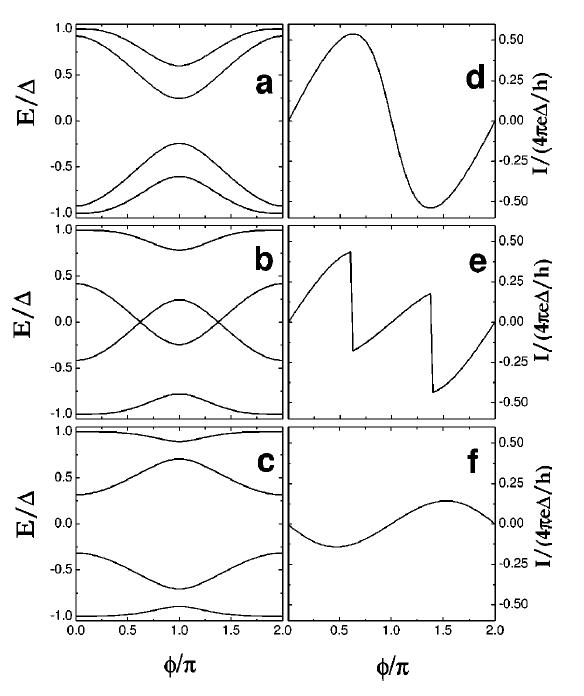
Figure 6: Evolution of the ABSs and Josephson current in the “toy” model of Ref. Vecino et al. (2003) for $\epsilon_{0}/\Gamma=-0.5$ and increasing $E_{ex}/\Gamma$ parameter: 0.25 (upper panels), 0.75 (middle panels) and 1.5 (lower panels). Reprinted figure with permission from E. Vecino et al., Physical Review B 68, 035105, 2003 Vecino et al. (2003). Copyright (2003) by the American Physical Society.

Further insight into the HFA solution can be provided by a ”toy” model introduced in Ref. Vecino et al. (2003) (A similar model was analyzed in Ref. Benjamin et al. (2007)). In this simplified model the finite magnetization which appears in the HFA is simulated by means of an exchange field parameter, $E_{ex}$, corresponding to the splitting of the diagonal dot levels for each spin, i.e. $\epsilon_{0\sigma}=\epsilon_{0}+\sigma E_{ex}$. The analysis of the Andreev states within this toy model is similar to the one given at the beginning of this section for the non-interacting case, and becomes particularly simple in the limit $\Delta\ll\Gamma$ in which they adopt the analytical expression

$$\left(\frac{\omega_{\pm}}{\Delta}\right)^{2}=\frac{\cos^{2}{\phi/2}+2E^{2}+Z^{2}(Z^{2}+\sin^{2}{\phi/2})\pm 2XS(\phi)}{Z^{4}+2(X^{2}+E^{2})+1},$$

(17)

where $E=\epsilon_{0}/2\Gamma$, $X=E_{ex}/2\Gamma$ and $Z^{2}=X^{2}-E^{2}$ and $S(\phi)$ is given by

$$S(\phi)=\sqrt{Z^{2}\cos^{2}{\phi/2}+E^{2}+\sin^{2}{\phi}/4}.$$

This expression clearly shows that the effect of the exchange field is to break the spin degeneracy producing an splitting of the ABSs. Consequently for $E_{ex}\neq 0$ one could in principle observe up to four ABSs in the spectral density. The evolution of these states with increasing $E_{ex}$ is shown in Fig. 6 together with the corresponding Josephson current. While for $E_{ex}<\Gamma$ the splitting is small and states corresponding to different spin orientation do not cross, for increasing $E_{ex}$ the upper and lower states closer to the Fermi energy begin to cross yielding a current-phase relation of $0^{\prime}$ or $\pi^{\prime}$ character. Eventually for sufficiently large $E_{ex}$ these two states completely interchange position with a complete reversal of the sign of the current ($\pi$-phase). It should be mentioned that although in this toy model the spin degeneracy is artificially broken, it nevertheless qualitatively simulates the behavior of the exact solution in the magnetic phase.

Another simple approach of a mean field type is provided by the slave boson mean field approximation (SBMFA). This method was introduced by Coleman for the normal Anderson model Coleman (1984); Hewson (1993). It is based in the introduction of auxiliary boson fields $b^{\dagger}_{0},b_{0}$ which act as projectors onto the empty impurity state. At the same time fermion creation and annihilation operators $f^{\dagger}_{0\sigma},f_{0\sigma}$ are introduced for describing the singly occupied states. In order to get rid of the doubly occupied states in the $U\rightarrow\infty$ these operators should satisfy the completeness relation

$$b^{\dagger}_{0}b_{0}+\sum_{\sigma}f^{\dagger}_{0\sigma}f_{0\sigma}=1$$ (18)

In terms of these operators the terms $H_{QD}$ and $H_{T}$ become

$$H_{QD} = \sum_{\sigma}\epsilon_{0}f^{\dagger}_{0\sigma}f_{0\sigma}$$

$$H_{T} = \sum_{k\sigma,\nu}\left(V_{k\nu}c^{\dagger}_{k\nu,\sigma}b^{\dagger}_{0}f_{0\sigma}+\mbox{h.c.}\right).$$ (19)

So far this transformation is exact in the $U\rightarrow\infty$ limit. Specific diagrammatic methods to obtain the impurity self-energy in this slave boson formulation have been developed Bickers (1987). Within this formulation the simplest solution is provided by the mean field approximation in which the boson operator is treated as a c-number. In fact the dot Hamiltonian reduces in this case to

$$H^{MF}_{QD} = \sum_{\sigma}\epsilon_{0}f^{\dagger}_{0\sigma}f_{0\sigma}+\lambda\left(|b_{0}|^{2}+\sum_{\sigma}f^{\dagger}_{0\sigma}f_{0\sigma}-1\right),$$

where $\lambda$ is a Lagrange multiplier associated to the constraint (18). The problem becomes equivalent to a non-interacting impurity model with renormalized parameters $\tilde{\epsilon}_{0}=\epsilon_{0}+\lambda$ and $\tilde{\Gamma}_{\nu}=|b_{0}|^{2}\Gamma_{\nu}$. Self-consistency is achieved by minimizing the system free energy.

Strictly speaking the mean field approximation is only valid in the $N\rightarrow\infty$ limit where $N$ is the level degeneracy of the Anderson model (for the single level case N=2). However, the mean field approximation yields a reasonably good description of quantities like the Kondo temperature in the normal case Hewson (1993). When applied to the Anderson model with superconducting electrodes the SBMFA is only valid in the regime $T_{K}\gg\Delta$ as it is not able to describe the transition to the $\pi$-phase when $T_{K}\sim\Delta$. In the regime $T_{K}\gg\Delta$ the ABSs as described by the SBMFA corresponds to the non-interacting case with renormalized parameters $\tilde{\epsilon}_{0}$ and $\tilde{\Gamma}$. In this way the ABSs within the SBMFA in this regime would be given by $\omega_{s}(\phi)=\pm\sqrt{1-\tilde{\tau}\sin^{2}\phi/2}$ with $\tilde{\tau}=4T_{K}^{2}/(\tilde{\epsilon}_{0}^{2}+4T_{K}^{2})$. In principle, the self-consistent effective parameters in the superconducting state can differ from those in the normal state. However, in the limit $T_{K}\gg\Delta$ in which the approximation is supposed to work this difference can be neglected. The SBMFA in the $U\rightarrow\infty$ limit has only been applied for the case of superconducting leads in a few references: Avishai et al. Avishai et al. (2003) for analyzing the dc current with an applied bias voltage, and in Ref. Yeyati et al. (2003) for studying the dynamics of Andreev states in the Kondo regime. Both works correspond to the non-equilibrium situation which will be discussed in Section V.

For a proper description of the phase-diagram within a mean-field slave boson approach a finite-$U$ version of the method, like the one introduced by Kotliar and Ruckenstein Kotliar and Ruckenstein (1986), is necessary. Within this method the number of auxiliary boson fields is extended up to four, denoted by $e,p_{\sigma}$ and $d$, which project into the empty, singly occupied (with either spin orientation) and doubly occupied dot states respectively. These operators must satisfy the constraints

$$\sum_{\sigma}p^{\dagger}_{\sigma}p_{\sigma}+e^{\dagger}e+d^{\dagger}d=1$$

$$c^{\dagger}_{0\sigma}c_{0\sigma}=p^{\dagger}_{\sigma}p_{\sigma}+d^{\dagger}d.$$ (21)

For recovering the non-interacting limit it is necessary to introduce also an auxiliary operator $z_{\sigma}=(1-d^{2}-p_{\sigma}^{2})^{-1/2}(ep_{\sigma}+p_{\bar{\sigma}}d)(1-e^{2}-p_{\bar{\sigma}}^{2})^{-1/2}$, in terms of which the model Hamiltonian becomes

$$H = H_{L}+H_{R}+\sum_{\sigma}\epsilon_{0}\hat{f}_{0\sigma}^{\dagger}\hat{f}_{0\sigma}+Ud^{\dagger}d+\sum_{k\nu,\sigma}\left(V_{k\nu}z_{\sigma}^{\dagger}\hat{f}_{0\sigma}^{\dagger}c_{k\nu\sigma}+h.c.\right)$$ (22)

$$-\lambda\left(e^{\dagger}e+d^{\dagger}d+\sum_{\sigma}p_{\sigma}^{\dagger}p_{\sigma}-1\right)-\sum_{\sigma}\lambda_{\sigma}\left(f_{0\sigma}^{\dagger}f_{0\sigma}-p_{\sigma}^{\dagger}p_{\sigma}-d^{\dagger}d\right),$$

where $\lambda$ and $\lambda_{\sigma}$ are the Lagrange multipliers associated with the constraints (21). Again, in a mean field approximation, the auxiliary fields are treated as c-numbers to be determined self-consistently.

The type of phase-diagram that is obtained within the finite-U SBMFA will be analyzed in subsection III.4, for the zero band-width limit which allows a comparison with exact diagonalizations. As it is shown in that subsection the finite-U SBMFA tends to underestimate the stability of the $\pi$-phase in contrast with the HFA, which typically overestimates it.

Another relatively simple approach is provided by the use a variational wave-function. This approach was used by Rozhkov and Arovas Rozhkov and Arovas (2000) extending previous works Varma and Yafet (1976) in which variational wave-functions were proposed for analyzing the normal Kondo problem. In their work Rozhkov and Arovas propose different many-body variational states in the $U\rightarrow\infty$ limit for the singlet and the doublet states, looking for the their relative stability. They find a transition between both ground states for $\Delta/T_{K}\sim 2$ and also predict the appearance of the intermediate phases $0^{\prime}$ and $\pi^{\prime}$ in addition to the pure $0$ and $\pi$ ones.

III.3 Diagrammatic approaches

III.3.1 Perturbation theory in the Coulomb interaction

A natural extension over the HFA is provided by applying diagrammatic perturbation theory in the Coulomb parameter $U$. Already at the level of second order one can obtain an approximation for the self-energy which is able to capture part of the interplay between Kondo effect and pairing interactions. This approximation has been applied both for the S-QD-S case in equilibrium Matsumoto (2001); Vecino et al. (2003), as well as for the N-QD-S case Cuevas et al. (2001); Yamada et al. (2010).

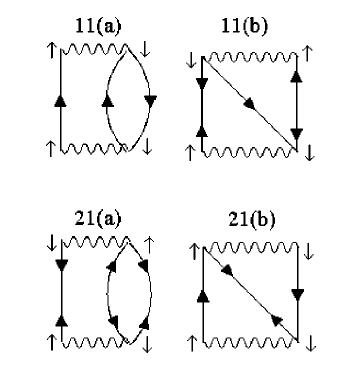
Figure 7: Feynmann diagrams for the second-order self-energy in the Anderson model with superconducting electrodes. Reprinted figure with permission from E. Vecino et al., Physical Review B 68, 035105, 2003 Vecino et al. (2003). Copyright (2003) by the American Physical Society.

The diagrams contributing to the second-order self-energy in the superconducting Anderson model are depicted in Fig. 7. The first diagrams (denoted as 11(a)) is equivalent to the one appearing in the normal case, describing interaction of an electron with an electron-hole pair with opposite spin. The other diagrams include anomalous superconducting propagators and are therefore characteristic of the superconducting state. The presence of these propagators gives several effects: the appearance of non-diagonal elements of the self-energy in Nambu space, and the presence of diagrams like 11(b) and 21(b) in Fig. 7 which corresponds to a double-exchange process. Finally, diagram 21(a) describes the interaction of a Cooper pair with fluctuations in the pairing amplitude within the dot.

Formally, these diagrams can be computed from the full Green functions of the non-interacting case by means of the expressions Vecino et al. (2003)

$$\Sigma^{r(2)}_{11,a}(\omega) = \frac{U^{2}}{(2\pi i)^{3}}\int d\epsilon_{1}\int d\epsilon_{2}\int d\epsilon_{3}\;\frac{G^{(0)+-}_{11}(\epsilon_{1})G^{(0)+-}_{22}(\epsilon_{2})G^{(0)-+}_{22}(\epsilon_{3})\,\,+\,\,G^{(0)-+}_{11}(\epsilon_{1})G^{(0)-+}_{22}(\epsilon_{2})G^{(0)+-}_{22}(\epsilon_{3})}{\omega-\epsilon_{1}-\epsilon_{2}+\epsilon_{3}+i0^{+}},$$

$$\Sigma^{r(2)}_{11,b}(\omega) = \frac{U^{2}}{(2\pi i)^{3}}\int d\epsilon_{1}\int d\epsilon_{2}\int d\epsilon_{3}\;\frac{G^{(0)+-}_{12}(\epsilon_{1})G^{(0)+-}_{21}(\epsilon_{2})G^{(0)-+}_{22}(\epsilon_{3})\,\,+\,\,G^{(0)-+}_{12}(\epsilon_{1})G^{(0)-+}_{21}(\epsilon_{2})G^{(0)+-}_{22}(\epsilon_{3})}{\omega-\epsilon_{1}-\epsilon_{2}+\epsilon_{3}+i0^{+}},$$

$$\Sigma^{r(2)}_{21,a}(\omega) = -\frac{U^{2}}{(2\pi i)^{3}}\int d\epsilon_{1}\int d\epsilon_{2}\int d\epsilon_{3}\;\frac{G^{(0)+-}_{21}(\epsilon_{1})G^{(0)+-}_{12}(\epsilon_{2})G^{(0)-+}_{21}(\epsilon_{3})\,\,+\,\,G^{(0)-+}_{21}(\epsilon_{1})G^{(0)-+}_{12}(\epsilon_{2})G^{(0)+-}_{21}(\epsilon_{3})}{\omega-\epsilon_{1}-\epsilon_{2}+\epsilon_{3}+i0^{+}},$$

$$\Sigma^{r(2)}_{21,b}(\omega) = \frac{U^{2}}{(2\pi i)^{3}}\int d\epsilon_{1}\int d\epsilon_{2}\int d\epsilon_{3}\;\frac{G^{(0)+-}_{22}(\epsilon_{1})G^{(0)+-}_{11}(\epsilon_{2})G^{(0)-+}_{21}(\epsilon_{3})\,\,+\,\,G^{(0)-+}_{22}(\epsilon_{1})G^{(0)-+}_{11}(\epsilon_{2})G^{(0)+-}_{21}(\epsilon_{3})}{\omega-\epsilon_{1}-\epsilon_{2}+\epsilon_{3}+i0^{+}}.$$

The evaluation of these expressions for a general range of parameters requires a significant numerical effort. An efficient algorithm can be implemented to evaluate these expressions based on Fast Fourier transformations, as discussed in Schweitzer and Czycholl (1990).

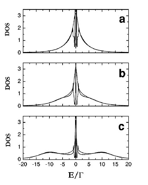
Figure 8: Evolution of the DOS in the S-QD-S system in equilibrium within the second-order self-energy approximation for and electron-hole symmetric case with $\Delta/\Gamma=0.1$. The $U/\Gamma$ parameter takes the values 2.5 (a), 5 (b) and 10 (c). Reprinted figure with permission from E. Vecino et al., Physical Review B 68, 035105, 2003 Vecino et al. (2003). Copyright (2003) by the American Physical Society.

In the limit $\Delta/\Gamma\ll 1$ Kondo correlations dominate over pairing ones. The results of the second-order self-energy approach for the half-filled case capture the main features of the onset of Kondo correlations in the spectral density when $U>\Gamma$. This is illustrated in Fig. 8 taken from Ref. Vecino et al. (2003), which shows its evolution for increasing $U/\Gamma$. The spectral density is similar to the one found in the normal state except for the superimposed features inside the superconducting gap. The overall shape evolves from the single Lorentzian broad resonance for $U<\Gamma$ to the three peaked structure characteristic of the Kondo regime when $U>\Gamma$. In this regime the width of the central Kondo peak is set by the scale $T_{K}$, which in the present approximation is given by $T_{K}\sim\Gamma/(1-\alpha_{0})$, where

$$\alpha_{0}=\frac{\partial\Sigma_{11}}{\partial\omega}(0)\simeq-\left(\frac{U}{2\pi\Gamma}\right)^{2}\left(3-\frac{\pi^{2}}{4}\right)\;,$$ (23)

thus coinciding with the perturbative result in the normal state (see Ref. Yamada and Yoshida (1975)). Although this perturbative approach fails to yield the exponential behavior of $T_{K}$ for large $U/\Gamma$, it provides a reliable description of the spectral density for moderate values of this parameter Ferrer et al. (1986).

The second-order self-energy allows also to analyze the renormalization of the ABSs due to the presence of Coulomb interactions. For values of $U/\Gamma<10$ the renormalized ABSs maintain approximately the $\sim\cos{\phi/2}$ behavior of the non-interacting case but with a narrower dispersion set by $\omega_{s}(0)\simeq\Delta\left[1-(U/U_{0})^{2}\right]$, where $(U_{0}/\Gamma)^{2}=(\Gamma/\Delta)\pi^{2}/(2\pi+2)$.

On the other hand, when $T_{K}\sim\Delta$ a transition to the $\pi$-phase is expected. Within the second-order self-energy approach the transition can be identified by allowing for a breaking of the spin-symmetry in the initial non-interacting problem and searching for self-consistency. Rather than imposing the consistency condition of the HFA, i.e. $\tilde{\epsilon}_{0\sigma}=\epsilon_{0}+U<n_{0\bar{\sigma}}>$ in Ref. Vecino et al. (2003) it was imposed that the effective dot level for each spin-orientation be determined by the charge-consistency condition, i.e. $<n_{0\sigma}>=<n^{0}_{0\sigma}>$, where $<n^{0}_{0\sigma}>$ is the dot charge corresponding to the broken-symmetry non-interacting Hamiltonian. Such a procedure was shown to eliminate the unstable behavior of perturbation theory when developed from the HFA Yeyati et al. (1993).

III.3.2 NCA approximation

Within the diagrammatic approximations one can include the so-called non-crossing approximation (NCA). In this case an infinite order resumation of the perturbation theory is performed starting from the $U\rightarrow\infty$ slave boson representation of the Anderson Hamiltonian Bickers (1987). To the lowest order in $1/N$ (where $N=2$ is the spin degeneracy) the family of diagrams in this resumation is represented in Fig. 9. The dashed lines correspond to the fermion propagators and the wavy lines to the slave bosons. In the normal case the NCA include only the first two diagrams in the Dyson equation for the fermion and boson propagators. The extension to the superconducting case was proposed in Ref. Clerk et al. (2000) and corresponds to including the anomalous propagators for describing multiple Andreev reflection processes (last two diagrams in the fermion and boson self-energies represented in Fig. 9).

Figure 9: Fermion (top) and boson (bottom) self-energy diagrams in the NCA approximation extended to the superconducting case. Reprinted figure with permission from G. Sellier et al., Physical Review B 72, 174502, 2005 Sellier et al. (2005). Copyright (2005) by the American Physical Society.

In the normal case the NCA theory has been shown to yield reliable results for temperatures down below $T_{K}$ Bickers (1987); Hewson (1993) in spite of certain pathologies like its failure to fulfill the Friedel sum-rule. The self-consistent extension for the superconducting case by Clerk et. al. Clerk and Ambegaokar (2000) is also formally exact to order $1/N$ and it is thus expected to yield reasonable results even in the presence of MAR processes.

Further analysis of the NCA applied to the S-QD-S system was provided in Ref. Sellier et al. (2005). Their results for the Josephson current and LDOS in the superconducting gap region are summarized in Fig. 10. The fact that the calculations are performed for temperatures which are a quite large fraction of $\Delta$ yields very broad resonances for the subgap states. As can be observed in Fig. 10, only one broad resonance can be clearly resolved within the gap. These results are in contrast to what is obtained using exact numerical methods as will be discussed in Sect. III.4.2. In this approximation the transition to the $\pi$-phase appears as a smooth crossover which can be associated to the crossing of this resonance through the Fermi energy.

Figure 10: Josephson current and subgap LDOS for the equilibrium S-QD-S model within the NCA for three values of $T_{K}/\Delta$ and three different temperatures. Reprinted figure with permission from G. Sellier et al., Physical Review B 72, 174502, 2005 Sellier et al. (2005). Copyright (2005) by the American Physical Society.

III.3.3 Real time diagrammatic approach

Another technique which has been applied to the study of quantum dots coupled to superconducting leads is the real time diagrammatic approach first introduced by König et al. König et al. (1996) for the normal Anderson model. The main idea of this technique is to integrate out the fermionic degrees of freedom of the electrodes leading to a reduced description of the density matrix projected on the Hilbert space of the isolated dot states. In the superconducting case this reduced density matrix also depends on the number of Cooper pairs in the leads relative to some chosen reference. The aim of the technique is to determine the time evolution of this reduced density matrix in the Keldysh contour thus allowing to consider both equilibrium and non-equilibrium situations. In Ref. Governale et al. (2008) the method has been applied to the equilibrium S-QD-S case obtaining results in agreement with those of Ref. Glazman and Matveev (1989) in the cotunneling limit. The method has been mainly applied to analyze the properties of quantum dots connected to both normal and superconducting leads in multiterminal configurations out of equilibrium, an issue which will be commented in Sect. VI.

III.4 Diagonalization by numerical methods

Within this subsection we will review methods which attempt a direct diagonalization of the superconducting Anderson model, either by truncating the initial Hilbert space using physical arguments valid for certain parameter region or by using the Numerical Renormalization group (NRG) method.

III.4.1 Exact diagonalization for the large $\Delta$ limit

An exact diagonalization of the model is possible in the limit $\Delta\rightarrow\infty$. In this limiting case the Hilbert space of the problem is automatically reduced to states spanned by the different electronic configuration of the dot levels. The effect of the superconducting leads appears as a pairing term between the electrons within the dot. The effective Hamiltionian for the truncated Hilbert space becomes Vecino et al. (2003); Tanaka et al. (2007b); T. Meng and Simon (2009)

$$H^{eff} = 2\Gamma\cos{\phi/2}\left(c_{0\uparrow}c_{0\downarrow}+c^{\dagger}_{0\downarrow}c^{\dagger}_{0\uparrow}\right)+\epsilon_{0}\sum_{\sigma}n_{0\sigma}$$ (24)

$$+Un_{0\uparrow}n_{0\downarrow}.$$

The eigenvalues of this reduced Hamiltonian can be determined straightforwardly by noting the decoupling of subspaces with even and odd number of electrons. The ground state for the even case (corresponding to total spin $S=0$) is a linear combination of the empty and doubly occupied dot state with an energy

$$E_{0(S=0)}(\phi)=\epsilon_{0}+U/2-\sqrt{(\epsilon_{0}+U/2)^{2}+4\Gamma^{2}\cos^{2}{\phi/2}}.$$ (25)

On the other hand, the odd number subspace simply corresponds to a single uncoupled spin with energy $E_{0(S=1/2)}=\epsilon_{0}$. The transition to the magnetic ground state thus occurs for $E_{0(S=1/2)}=E_{0(S=0)}(\phi)$. In the simpler electron-hole symmetric case $(\epsilon_{0}=-U/2)$ this condition reduces to $2\Gamma\cos{\phi/2}=U/2$ and thus the full $\pi$ state appears for $\Gamma<U/4$. This simple model already gives a rough qualitative account of the $0-\pi$ quantum phase transition.

A further step in the idea truncating the Hilbert space is performed in the so called zero band-width limit Affleck et al. (2000); Vecino et al. (2003); Bergeret et al. (2007). In this approximation the superconducting leads are represented by a single localized level (which formally corresponds to the limit of vanishing width of the leads spectral density). This approximation is justified when the superconducting gap is large compared to the other energy scales in the problem, and thus can be considered as a refinement with respect to the previous approach. The corresponding Hamiltonian can be written as $H=H_{d}+H_{T}+H_{L}+H_{R}$, with

$$H_{\nu} = \sum_{\sigma}\epsilon_{\nu}c^{\dagger}_{\nu\sigma}c_{\nu\sigma}+\left(\Delta_{\nu}c_{\nu\uparrow}c_{\nu\downarrow}+\mbox{h.c.}\right)$$

$$H_{T} = \sum_{\nu,\sigma}\left(V_{\nu}c^{\dagger}_{\nu\sigma}c_{0\sigma}+\mbox{h.c.}\right),$$ (26)

where $\nu=L,R$ denotes the left-right sites describing the leads in this approximation.

Although the total number of particles is not a good quantum number, their parity is conserved as in the previous case. This allows to reduce the initial 64 states in the Hilbert space to a subspace of 20 states for even parity with a total spin $z$-component $S_{z}=0$ and 15 states for odd parity with $S_{z}=\pm 1/2$. These values of $S_{z}$ are the ones corresponding to the ground state in each subspace with total spin $S=0$ and $S=1/2$. In addition to providing a qualitative description of the phase diagram of the full model, this simplified calculation can furthermore be useful as a test for comparing different approximation methods.

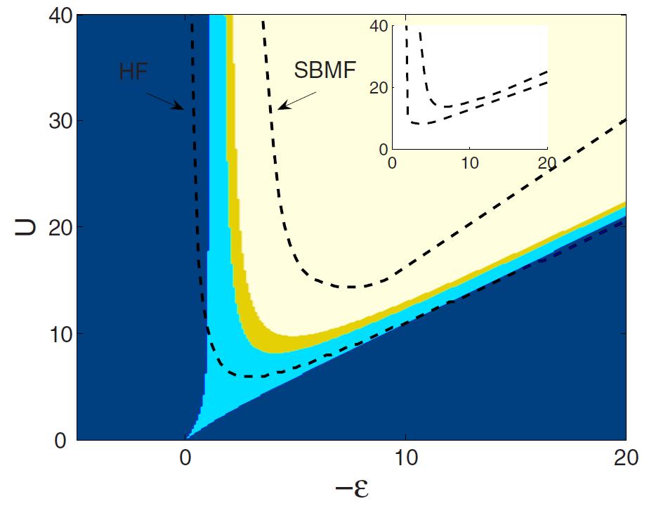
Figure 11: Phase diagram of the S-QD-S system in the ZBW model for the leads obtained by exact diagonalization for $\Delta=V_{L}=V_{R}$, taken as unit of energy. The dashed lines correspond to the boundary between the 0 and $\pi$ regions within the HFA (lower line) and the finite-U SBMFA (upper line). The inset show the corresponding results for these boundaries within the full model. Reprinted figure with permission from F.S. Bergeret et al., Physical Review B 76, 174510, 2007 Bergeret et al. (2007). Copyright (2007) by the American Physical Society.

The phase diagram obtained within this approximation was discussed in Refs. Vecino et al. (2003); Bergeret et al. (2007) and is shown in Fig. 11 for $\Gamma\equiv V=\Delta$, with $V_{L}=V_{R}=V$. As can be observed, the overall diagram is very similar to the one shown before for the HFA (Fig. 5) exhibiting the four phases $0,0^{\prime},\pi^{\prime}$ and $\pi$ in the same sequence. For a more direct comparison it is necessary to perform the HFA of the ZBW model, which as an exactly solvable model also provides a stringent test of the approximation. The lower broken line in Fig. 11 indicates the boundary of the $\pi$-phase within the HFA. It can be noticed that the HFA overestimates the stability of this magnetic phase. On the other hand, it is also possible to test the finite-U SBMF approximation in this ZBW model. The corresponding boundary for the $\pi$-phase is indicated by the upper broken line in Fig. 11. In opposition to the HFA this approximation overestimates the stability of the $0$ phase, the exact boundary therefore lying in between the two different mean-field approximations. It is interesting to point out that a similar difference between both approximations is also found for the full model (see inset in Fig. 11). One would then expect that the exact boundary for the full model lays in between these two.

Figure 12: Ground state energy for the $S=0$ and $S=1/2$ states of the S-QD-S system in the ZBW model for the leads. Full lines correspond to the exact results, dotted lines to the HFA and dashed lines to the second-order self-energy approximation. Reprinted figure with permission from E. Vecino et al., Physical Review B 68, 035105, 2003 Vecino et al. (2003). Copyright (2003) by the American Physical Society.

The ZBW model can also be used to test approximate methods beyond the mean field ones. In Ref. Vecino et al. (2003) this was done for the second-order self-energy approximation. As it is illustrated in Fig. 12 for the symmetric case $(\epsilon_{0}=-U/2)$ the second-order self-energy approach matches quite well the exact ground state energy for $U/\Delta$ values up to $\simeq 2.5$. It is interesting to note that for larger $U$ values even when the HFA already yields a full $\pi$-state, the second-order approximation predicts a mixed ground state in agreement with the exact solution.

III.4.2 Numerical Renormalization Group (NRG)

The NRG method is based on the ideas of Wilson on logarithmic discretization for magnetic impurity problems Wilson (1975) and was first applied to the Anderson model by Krishna-murthy et al. Krishna-murthy et al. (1980). The idea behind the method is to discretize the energy levels in the leads on a logarithmic grid of energies $\Lambda^{-n}$ (with $\Lambda>1$ and $1\leq n\leq N\rightarrow\infty$) with exponentially high resolution on the low-energy excitations. This discretization allows then to map the impurity model into a linear ”tight-binding” chain with hopping matrix elements decaying as $\Lambda^{-n/2}$ with increasing site index $n$. The sequence of Hamiltonians which is constructed by adding a new site in the chain is then diagonalized iteratively. As the number of states grows exponentially an adequate truncation scheme is required.

The NRG scheme has been first generalized to the case of an Anderson impurity in a superconducting host by Yoshioka and Ohashi Yoshioka and Ohashi (2000) and implemented by several authors to analyze the S-QD-S model with a finite phase difference Choi et al. (2004); Oguri et al. (2004); Tanaka et al. (2007b); Lim and Choi (2008). For the left-right symmetric case (i.e. $\Delta_{L}=\Delta_{R}$ and $\Gamma_{L}=\Gamma_{R}$) the sequence of Hamiltonians can be written as Choi et al. (2004)

$$\tilde{H}_{N+1} = \sqrt{\Lambda}\tilde{H}_{N}+\xi_{N}\sum_{\mu,\sigma}\left(f^{\dagger}_{\mu,N+1,\sigma}f_{\mu,N+1,\sigma}+\mbox{h. c.}\right)$$ (27)

$$-\Lambda^{N/2}\sum_{\mu}\tilde{\Delta}_{\mu}\left(f^{\dagger}_{\mu,N+1,\uparrow}f^{\dagger}_{\mu,N+1,\downarrow}+\mbox{h. c.}\right),$$

where the initial Hamiltonian is given by

$$\tilde{H}_{0} = \frac{1}{\sqrt{\Lambda}}\left[\tilde{H}_{QD}+\sum_{\mu=e,o}\sum_{\sigma}\tilde{V}_{\mu}\left(c^{\dagger}_{0\sigma}f_{\mu,0,\sigma}+\mbox{h. c.}\right)\right.$$ (28)

$$\left.-\sum_{\mu}\tilde{\Delta}_{\mu}\left(f^{\dagger}_{\mu,0,\sigma}f_{\mu,0,\sigma}+\mbox{h. c.}\right)\right].$$

The fermion operators $f_{\mu,N,\sigma}$ correspond to an effective tight-binding chain resulting from the logarithmic discretization and the canonical transformation into the even-odd linear combination of original left-right states in the leads and

$$\tilde{H}_{QD} \equiv \chi\frac{H_{QD}}{D}\;\;\;,\;\;\;\tilde{\Delta}_{\mu}\equiv\chi\frac{\Delta_{\mu}}{D}$$ (29)

$$\tilde{V}_{e} = \chi\sqrt{\frac{2\Gamma}{\pi D}}\cos{\phi/4}\;\;,\;\;\tilde{V}_{o}=-\chi\sqrt{\frac{2\Gamma}{\pi D}}\sin{\phi/4},$$

with $\chi=2/(1+1/\Lambda)$ and $D$ being an energy cut-off in the leads spectral density. The original Hamiltonian is recovered in the limit $H/D=\lim_{\rightarrow\infty}\tilde{H}_{N}/(\chi\Lambda^{(N-1)/2})$.

Figure 13: Phase diagram of the S-QD-S system in the $\Gamma_{R},\epsilon_{0}$ plane for fixed $U$ and different values of $\Gamma_{L}/\Gamma_{R}$ obtained using the NRG method. Reprinted figure with permission from Y. Tanaka et al., New Journal of Physics 9, 115, 2007 Tanaka et al. (2007b). Copyright (2007) by IOP Publishing Ltd.

The NRG method was applied to analyzing the Josephson current in a S-QD-S system in Ref. Choi et al. (2004), this work confirming the predicted $0-\pi$ quantum phase transition at $\Delta\sim T_{K}$ for the electron-hole symmetric case. It should be mentioned that more recent calculations Karrasch et al. (2008) using NRG obtain Josephson currents which are approximately a factor 2 larger than the ones of Choi et al. (2004). On the other hand, Oguri et al. Oguri et al. (2004) used NRG to analyze this model in the case of $|\Delta_{L}|\gg|\Delta_{R}|$. In this case the model can be exactly mapped into a single channel model consisting on the right lead coupled to the Anderson impurity with a local pairing $\Delta_{d}\equiv\Gamma_{L}e^{i\phi_{L}}$, thus allowing a simpler implementation of the NRG algorithm. Further work for the $\Gamma_{L}\neq\Gamma_{R}$ case although with $\Delta_{L}=\Delta_{R}$ by Tanaka et al. Tanaka et al. (2007b) confirmed the presence of intermediate $0^{\prime}-\pi^{\prime}$ phases even in the left-right asymmetric case. A characteristic phase diagram obtained for this case is shown in Fig. 13.

In addition to the ground state properties, NRG methods have been applied in an attempt to clarify the structure of the subgap ABSs. In Ref. Lim and Choi (2008) the spectral density inside the gap obtained from the NRG algorithm was analyzed, showing that a pair of ABSs located symmetrically respect to the Fermi energy is present in the $U\rightarrow\infty$ case. This is in contrast to the NCA results discussed previously (shown in Fig. 10) where a single broad resonance appears. Similar conclusions are obtained in Ref. Bauer et al. (2007) although for the single lead case and for finite $U$. A word of caution should be said regarding the analysis of the ABSs in this last work in which the relation $\Sigma_{22}(\omega)=-\Sigma_{11}(-\omega)$ is assumed in their Eq. (8) for the states inside the gap. This relation would not be strictly valid for the doublet ground state when choosing a given spin orientation. In this case the quasi-particle excitation energies would become spin dependent and the electron-hole symmetry would be broken. This would allow in principle to have up to 4 ABSs inside the gap as predicted both by the Hartree-Fock approximation and in the exact $\Delta\rightarrow\infty$ limit. Of course, in the $\pi$ phase the spin is not frozen but is fluctuating. In this sense the above relation between the self-energy components would be recovered when averaging over the $S_{z}=1/2$ and $S_{z}=-1/2$ states. We believe in any case that a more detailed analysis of the ABSs using the NRG method is still lacking.

III.5 Functional renormalization group

Figure 14: Current phase-relations for the S-QD-S system obtained using the fRG approach truncated at the HF level for different values of $U/\Gamma$ and $\Delta/\Gamma$. For comparison the results obtained using the NRG method are also plotted (indicated by the filled dots). Reprinted figure with permission from C. Karrash et al., Physical Review B 77, 024517, 2008 Karrasch et al. (2008). Copyright (2008) by the American Physical Society.

The functional renormalization group (fRG) method is based on the application of an RG analysis to the diagrammatic expansions in terms of electronic Green functions. This is an approximate method whose accuracy depends on the initial diagrams used in the evaluation of the electron self-energies. The starting point is the introduction of an energy cut-off $\Lambda$ into the Matsubara non-interacting Green-functions

$$G^{0,\Lambda}(i\omega)=\Theta(|\omega|-\Lambda)G^{0}(i\omega)$$

Using these propagators the $n-$particle vertex functions acquires a $\Lambda$ dependence. The flow equations are determined differentiating these vertex functions with respect to $\Lambda$ which are then solved iteratively for increasing $\Lambda$. In Ref. Karrasch et al. (2008) the method has been applied to the S-QD-S system employing a truncation scheme which keeps only diagrams corresponding the the static Hartree-Fock approximation. The $\Lambda$-dependent Green function used in Ref. Karrasch et al. (2008) was of the form,

$$G^{\Lambda}(i\omega)=\left(\begin{array}[]{cc}i\tilde{\omega}-\epsilon_{0}-\Sigma^{\Lambda}&\tilde{\Delta}(i\omega)-\Sigma^{\Lambda}_{\Delta}\\ \tilde{\Delta}(i\omega)-\Sigma^{\Lambda}_{\Delta}&i\tilde{\omega}+\epsilon_{0}+\Sigma^{\Lambda}\end{array}\right)^{-1},$$ (30)

where $i\tilde{\omega}=i\omega(1+\sum_{\mu}\Gamma_{\mu}g(i\omega))$ and $\tilde{\Delta}(i\omega)=\sum_{\mu}\Gamma_{\mu}f(i\omega)e^{i\phi_{\mu}}$, $g$ and $f$ being the dimensionless BCS Matsubara Green functions of the uncoupled leads. Within this approximation the flow equations lead to energy-independent self-energies, corresponding to an effective non-interacting model with renormalized parameters. It is important to notice that this approximation exhibits also the limitation already pointed out in the previous section as it imposes electron-hole symmetry which is not satisfied in the magnetic phase. Nevertheless the approximation allows to identify a transition to a phase with inversion of the Josephson current which is driven by an ”overscreening” of the induced pairing determined by $\Sigma_{\Delta}$. Fig. 14 shows the comparison of fRG results with those obtained with the NRG method. The agreement is rather good for large $\Delta/\Gamma$ but it becomes poorer in the $\pi$-phase. We believe that the agreement could be improved allowing for a broken symmetry state within the same fRG approach.

III.6 Quantum Monte-Carlo

The Josephson current in the S-QD-S system has also been analyzed using Quantum Monte Carlo (QMC) simulations by Siano and Egger Siano and Egger (2004). The method used was the Hirsh-Fisher algorithm adapted to this particular problem. They consider the deep Kondo regime $U/\Gamma\gg 1$ and $\epsilon_{0}/\Gamma\ll-1$ and show that the results for the Josephson current exhibit a universal dependence with $T_{K}$ provided that $U/\Gamma>5$. They identify the transition between the different phases at $\Delta/T_{K}\simeq 0.51,0.875$ and $1.105$ for $0-0^{\prime}$, $0^{\prime}-\pi^{\prime}$ and $\pi^{\prime}-\pi$ respectively Siano and Egger (2005a). Being a finite temperature calculation the resulting current-phase relations do not exhibit sharp discontinuities in the intermediate phases. This smooth behavior was criticized in Ref. Choi et al. (2005a) pointing out that the QMC results did not match the NRG ones of Ref. Choi et al. (2004) at finite temperatures, which was attributed by Siano and Egger in their reply Siano and Egger (2005b) to a possible limited accuracy of the NRG calculation of Ref. Choi et al. (2004). More recent NRG calculations of Ref. Karrasch et al. (2008) give a good agreement with QMC results at finite temperature for $\phi$ values between $\pi/2$ and $\pi$, whereas QMC underestimates the current in the range $0-\pi/2$. It is claimed in Ref. Karrasch et al. (2008) that the origin of the discrepancy lies in the fact that the first excited state in this phase range is smaller or of the order of the temperature values used in the calculations of Siano and Egger (2004).

The QMC method has more recently been applied to analyze the spectral properties of this model in Ref. Luitz and Assaad (2010). The authors employ the so-called weak-coupling continuous-time version of the method which is based on a perturbative expansion around the $U=0$ limit. They show that the results for the spectral densities are in qualitative good agreement with the ones obtained in the zero band-width approximation introduced in Ref. Vecino et al. (2003), which was discussed before in this section.

III.7 Experimental results

Several physical realizations of the S-QD-S system have been obtained in the last few years by means of contacting carbon nanotubes (CNT), C60 molecules or semiconducting nanowires with superconducting electrodes (for a recent review see Ref. Franceschi et al. (2010)). In view of the existence of this review on the experiments in this section we give only a brief summary of the main findings and its relation to the theoretical work.

CNTs have provided so far the most promising setups for a direct test of the theoretical predictions concerning the Josephson effect through a QD. The first experiments detecting a supercurrent through a CNT-QD strongly coupled to the leads (i.e. $\Gamma\gg\Delta,U$) were performed by Jarillo-Herrero et al Jarillo-Herrero et al. (2006). These experiments were basically performed in the resonant-tunneling regime with a single-level spacing $\delta\epsilon\gg\Gamma$. The results indicated a strong correlation between the critical current $I_{c}$ and the normal conductance $G_{N}$. However, the product $I_{c}R_{N}$ deviated from a constant value due to the effect of the electromagnetic environment suppressing the critical current more strongly in off-resonance conditions due to phase fluctuations.

Figure 15: Experimental setup used in Ref. Cleuziou et al. (2006) for analyzing the $0-\pi$ transition in CNT QDs (upper panel). The middle panel shows the reversal of the oscillatory pattern of the current as a function of the magnetic flux through the SQUID across the transition. The lower panel shows the correlation of the $\pi$-phase region with the Kondo ridges in the normal state (indicated by the dashed line). Reprinted by permission from Macmillan Publishers Ltd: Nature Physics Cleuziou et al. (2006), copyright (2006).

In a subsequent work by the same group the first experimental evidence of $\pi$-junction behavior in a S-QD-S system was obtained using semiconducting InAs nanowires with Al leads in a SQUID configuration van Dam et al. (2006). However, the observed features in this experiment could not be explained completely on the basis of a single-level model but rather a multilevel description was necessary. In particular the authors showed that in this case the $\pi$-junction behavior is not necessarily linked to the parity of the number of the electrons in the dot (this will be further discussed in Sect. VI). On the other hand, $\pi$-junction behavior have also been demonstrated in Ref. Cleuziou et al. (2006) using CNT-QDs in a SQUID geometry. The corresponding experimental setup is depicted in Fig. 15. In this SQUID configuration the transition to the $\pi$-phase is directly demonstrated in the measured current-phase relation as a function of one of the applied gate voltages (see Fig. 15). Remarkably, this experiment allows to correlate the appearance of the $\pi$-junction behavior with the presence of Kondo correlations in the normal state. The dotted lines in the lower panel of Fig. 15 indicate the Kondo ridge appearing in the normal state (which is recovered by applying a magnetic field).

Evidence of a $0-\pi$ transition has also been found in CNT-QD systems by analyzing the current-voltage characteristic Jorgensen et al. (2007). In this work it was shown that the evolution of the zero-bias conductance can be correlated to the behavior of the critical current when transversing the $0-\pi$ boundary. As it corresponds to a non-equilibrium situation this analysis will be discussed later in Sect. V. A similar observation holds for other experimental works Vecino et al. (2004); Grove-Rasmussen et al. (2007); Eichler et al. (2009) which will be discussed in that section.

Figure 16: Color scale plots of the local density of states in a CNT QD coupled to SC leads as reported in Ref. Pillet et al. (2010) as a function of gate voltage and phase difference. The figure also shows the results obtained from a phenomenological model, as discussed in the text. Reprinted by permission from Macmillan Publishers Ltd: Nature Physics Pillet et al. (2010), copyright (2010).

Finally, it is worth pointing out recent experimental developments which have allowed to directly measure the Andreev bound states spectrum of a CNT-QD coupled to superconducting leads in a SQUID configuration Pillet et al. (2010). In this experiment a weakly coupled lead was deposited at the center of the CNT to allow for tunneling spectroscopy measurements. In this way both the phase and gate voltage variation of the Andreev bound states were determined. The results could be fitted satisfactorily using a simplified phenomenological model corresponding to the superconducting Anderson model within a mean field approximation, in which an exchange field is included to represent the magnetic ground state. An example of the comparison between theory and experiment is given in Fig. 16. This analysis showed that a double dot model was in general necessary to fit the experimental results. Recent experimental work on graphene QDs coupled to SC leads Dirks et al. (2011) provided also evidence on the crossing of ABs as a function of the gate potential which is consistent with a magnetic ground state.

IV Quantum dots with normal and superconducting leads

A single-level quantum dot coupled to a normal and a superconducting lead provides a basic model system to study electron transport in the presence of Coulomb and pairing interactions. Compared to the S-QD-S situation, this case has a simpler response in non-equilibrium conditions due to the absence of the ac Josephson effect. For this reason this system has been widely analyzed theoretically.

As in any N-S junction the low bias transport properties are dominated by Andreev processes. This mechanism is in general highly modified by resonant tunneling through the localized levels in the dot. In addition, charging effects can strongly suppress the Andreev reflection in certain parameter ranges. Furthermore there is also an interesting interplay between Kondo and pairing correlations as in the case of the S-QD-S system discussed above.

As an illustration of the general formalism we derive here the linear transport properties of the non-interacting model. One can straightforwardly write the dot retarded Green function for this case from expression (11) by setting $\Delta_{L}=0$. Then, from the expression of the current in terms of Keldysh Green functions and using the corresponding Dyson equation one can write

$$I_{L} = \frac{e}{h}\sum_{k}\int d\omega\mbox{Tr}\left[\tau_{3}\left(V_{kL}\hat{g}^{+-}_{kL}V_{Lk}\hat{G}^{-+}_{00}\right.\right.$$ (31)

$$\left.\left.-V_{kL}\hat{g}^{-+}_{kL}V_{Lk}\hat{G}^{+-}_{00}\right)\right],$$

where $\hat{g}_{kL}^{+-,-+}$ are the Keldysh Green functions of the uncoupled normal lead. By further using $G^{+-,-+}_{00}=\sum_{\mu,k}G^{r}_{00}V_{\mu k}\hat{g}_{k\mu}^{+-,-+}V^{*}_{\mu k}\hat{G}^{a}_{00}$ and taking the wide band approximation for the uncoupled leads one can obtain the following expression for the temperature dependence linear conductance Schwab and Raimondi (1999); Cuevas et al. (2001)

$$G=\frac{16e^{2}}{h}\Gamma_{N}\Gamma_{S}\int d\omega\mbox{Im}\left(G^{r}_{12}G^{a}_{11}\right)\left(-\frac{\partial n_{F}}{\partial\omega}\right)$$ (32)

which, at zero temperature reduces to the simple expression arising from the contribution of pure Andreev reflection processes

$$G=\frac{4e^{2}}{h}\frac{4\Gamma_{N}^{2}\Gamma_{S}^{2}}{\left(\epsilon_{0}^{2}+\Gamma_{N}^{2}+\Gamma_{S}^{2}\right)^{2}}$$ (33)

As shown in Ref. Beenakker (1992) this expression for the non-interacting case is equivalent to the formula $G=(4e^{2}/h)\tau^{2}/(2-\tau)^{2}$, with $\tau=4\Gamma_{N}\Gamma_{S}/(\epsilon_{0}^{2}+(\Gamma_{N}+\Gamma_{S})^{2})$ being the normal transmission through the dot at the Fermi energy. In contrast to the case of a NS quantum point contact with essentially energy independent transmission, in the dot case the Andreev processes become resonant at $\epsilon_{0}=0$ reaching the maximum value $G=4e^{2}/h$.

IV.1 Effect of interactions (linear regime)

One of the first attempts to describe the effect of Coulomb interactions in the NDQS system was presented by Fazio and Raimondi Fazio and Raimondi (1998) using the equation of motion technique truncated to the second order in the tunneling to the leads. They derived expressions for the mean current using the Keldysh formalism and extending the so-called Ng ansatz Ng (1993) to the superconducting case. The claim of an extended temperature range for the zero bias anomaly due to the Kondo resonance was subsequently corrected in Fazio and Raimondi (1999).

The problem was addressed in Ref. Kang (1998) by assuming that the relation $G=(4e^{2}/h)\tau^{2}/(2-\tau)^{2}$ of the non-interacting case still holds by substituting $\tau$ by the normal transmission of the interacting case. Within this assumption that work suggested an increase of the conductance in the Kondo regime by a factor of two with respect to the normal case. As shown by subsequent works which we discuss below, this enhancement is not always possible, the general case is rather the opposite.

The conductance of the interacting N-QD-S system was also analyzed in Ref. Schwab and Raimondi (1999) within the infinite-U slave-boson mean field approximation. This approximation reduces the problem into an effective Fermi liquid description with renormalized parameters $\tilde{\Gamma}_{N,S}$ and $\tilde{\epsilon}_{0}$. Within this approximation both $\Gamma_{N,S}$ are renormalized equally and therefore the condition for the maximum conductance is reached for the symmetric case as in the normal state. As the authors acknowledge this result is valid only in the deep Kondo regime $\Delta\ll T_{K}$, otherwise residual interactions would renormalize the left and right tunneling rates differently, in particular $\Gamma_{S}$ coupling the dot with the superconductor would be significantly suppressed by interactions.

The problem was subsequently addressed by Clerk et al. Clerk et al. (2000) using the extension of the NCA to the superconducting case already mentioned in Sect. III. They analyze three different models: the N-QD-S Anderson model and a single channel magnetic and a two-channel non-magnetic contact between normal and superconducting electrodes. We comment here only the results for the first model. They find an overall decrease of the quasiparticle spectral density at the Fermi energy together with the appearance of additional Kondo peaks at $\pm\Delta$. As a consequence, their conclusion was that there is no enhancement of the linear conductance due to Andreev processes in contrast to the claim of previous works.

Diagrammatic techniques for the finite-U N-QD-S Anderson model were applied in Ref. Cuevas et al. (2001). Within this approach the linear conductance can be expressed as the one corresponding to the non-interacting model with asymmetrically renormalized parameters

$$G=\frac{4e^{2}}{h}\frac{4\Gamma_{N}^{2}\tilde{\Gamma}_{S}^{2}}{\left(\tilde{\epsilon}_{0}^{2}+\Gamma_{N}^{2}+\tilde{\Gamma}_{S}^{2}\right)^{2}}$$ (34)

where $\tilde{\Gamma}_{S}=\Gamma_{S}-\Sigma_{12}(0)$ and $\tilde{\epsilon}_{0}=\epsilon_{0}-\Sigma_{11}(0)$, $\Sigma_{\mu,\nu}$ being the dot self-energy elements in Nambu space. Although this result is valid in general within a diagrammatic analysis, concrete results were obtained in this work by means of an interpolated second-order approach. From Eq. (34) it was found that even when the starting bare parameters correspond to the symmetric case $\Gamma_{N}=\Gamma_{S}$, interactions would tend to reduce the conductance by inducing an asymmetry, i.e. leading to $\tilde{\Gamma}_{S}\neq\Gamma_{N}$, as was suggested in Ref. Schwab and Raimondi (1999). However, this equation also predicts the possibility that an adequate tuning of the bare coupling parameters could yield an enhancement of the conductance up to the unitary limit ($4e^{2}/h$ in the NS case) which would not correspond to the maximum conductance in the normal case.

The approximation of Ref. Cuevas et al. (2001) is based on the evaluation of the second order diagrams, which due to the proximity induced pairing in the dot are formally the same as those of Fig. 7 which were discussed for the S-QD-S case. For the non-symmetric case the authors used an interpolative ansatz which recovers the correct behavior in the $\Gamma/U\rightarrow 0$ (atomic) limit. The obtained behavior of the conductance as a function of $U/\Gamma$ for the symmetric and non-symmetric cases is illustrated Fig. 17.

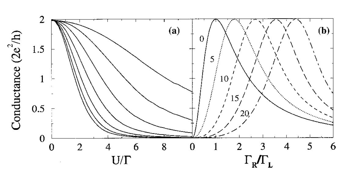
Figure 17: Linear conductance for the N-QD-S system in the second-order self-energy approximation of Ref. Cuevas et al. (2001). (a) symmetric case as a function of $U/\Gamma$ for different values of $\Gamma/\Delta=0.125,0.25,0.5,1.0,2.0,4.0$ and 8.0, from top to bottom. (b) Same as (a) for asymmetric coupling to the leads $\Gamma_{L}\neq\Gamma_{R}$ and different values of $U/\Gamma_{L}$ (within the text we have set $\Gamma_{L}\equiv\Gamma_{N}$ and $\Gamma_{R}\equiv\Gamma_{S}$). Reprinted figure with permission from J.C. Cuevas et al., Physical Review B 63, 094515, 2001 Cuevas et al. (2001). Copyright (2001) by the American Physical Society.

As can be observed, in the symmetric case the conductance drops steadily from the unitary limit as $U/\Gamma$ increases, the scale of this decay being set by the parameter $\Gamma/\Delta$. On the other hand the right panel of Fig. 17 illustrates that the unitary limit can be restored by an adequate tuning of the ratio $\Gamma_{N}/\Gamma_{S}$.

The behavior of the linear conductance in the N-QD-S was also analyzed in Krawiec and Wysokinski (2004); Domanski and Donabidowicz (2008) using the EOM technique with different decoupling schemes. While in Ref. Krawiec and Wysokinski (2004) it was obtained that the conductance due to Andreev processes was completely suppressed in the Kondo regime, an improved approximation for the EOM decoupling procedure in Ref. Domanski and Donabidowicz (2008) showed that there is in fact a finite zero bias anomaly in the Andreev conductance although it is in general much smaller than the one in the normal case, its value depending on the ratio $\Gamma_{N}/\Gamma_{S}$. This behavior is in qualitative agreement with the results of the diagrammatic approach discussed before. However, the unitary limit is not reached within this approach.

More recently the linear conductance of the N-QD-S model has been studied using the NRG method Tanaka et al. (2007a). In this work the limit $\Delta\rightarrow\infty$ was taken from the start, which allows to map the problem into the case of a QD with a local pairing amplitude $\Delta_{d}=\Gamma_{S}$ coupled to a single normal electrode (the $\Delta\rightarrow\infty$ limit for the S-QD-S case was discussed in Sect. III). The NRG algorithm can be considerably simplified by this assumption because a simple Bogoliubov transformation allows to get rid of the local pairing term leading to a problem which is formally equivalent to a normal Anderson model, which implies Fermi liquid behavior. As in the diagrammatic approach discussed before, the main effect of the interactions is to renormalize the couplings $\Gamma_{N,S}$ and the dot level position. Figure 18 illustrates the evolution of the renormalized parameters $\tilde{\Gamma}_{N,S}$ as a function of $U$ for the half-filled case $\epsilon_{0}=-U/2$ with initial parameters $\Gamma_{S}=5\Gamma_{N}$. As can be observed in the upper panel of Fig. 18, the main effect of increasing the interaction $U$ is to reduce the effective coupling to the superconductor, $\tilde{\Gamma}_{S}$, while the effective coupling to the normal lead $\tilde{\Gamma}_{N}$ remains almost constant up to the region $U\sim 10\Gamma_{N}$ when the Kondo effect is significant. Eventually the system reaches the condition $\tilde{\Gamma}_{N}\simeq\tilde{\Gamma}_{S}$ and the conductance increases up to the unitary limit, as shown in the lower inset of Fig. 18. This behavior is in good agreement with the prediction of the diagrammatic theory of Ref. Cuevas et al. (2001). On the other hand, the induced pairing amplitude (middle panel in Fig. 18), exhibits the expected monotonous decrease for increasing intradot repulsion.

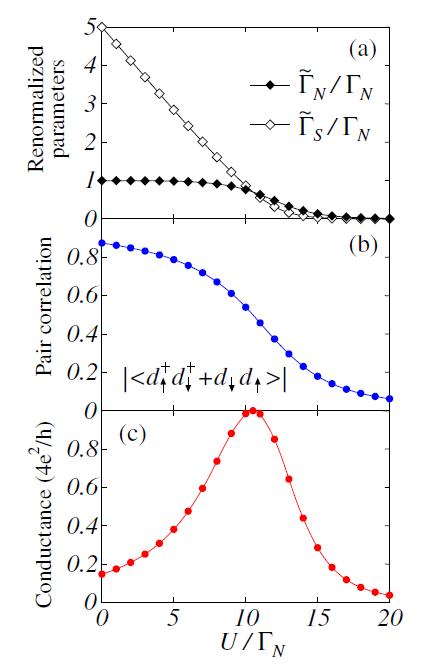
Figure 18: Renormalized couplings to the leads $\tilde{\Gamma}_{N,S}$ (upper panel); Induced pairing amplitude (middle panel) and linear conductance (lower panel) as a function of $U/\Gamma_{N}$ for the N-QD-S system obtained using NRG method in the $\Delta\rightarrow\infty$ limit. Reprinted figure with permission from Y. Tanaka et al., Journal of the Physical Society of Japan 76, 074701, 2007 Tanaka et al. (2007a). Copyright (2007) by the Physical Society of Japan.

The behavior of the linear conductance outside the half-filled case obtained from these NRG calculations is illustrated in Fig. 19. In this color-scale map it can be clearly observed that the unitary limit is reached mainly along the curve $((\epsilon_{0}/U+1/2)^{2}+(\Gamma_{S}/U)^{2})^{1/2}=1/2$, which corresponds to the single-doublet transition in the $\Gamma_{N}\rightarrow 0$ limit. When $\Gamma_{S}/U<0.5$ (corresponding to the doublet state in the $\Gamma_{N}\rightarrow 0$ limit within the dashed curve in Fig. 19), the conductance as a function of $\epsilon_{0}$ exhibits a double peaked structure, whereas for $\Gamma_{S}/U>0.5$ only a single peak is found which can be correlated to the superconducting singlet ground state of the system in the $\Gamma_{N}\rightarrow 0$ limit.

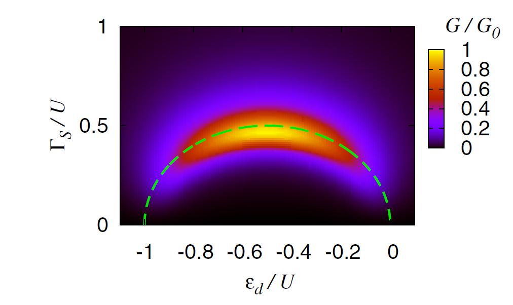
Figure 19: Color-scale map of the linear conductance in the N-QD-S system in the $\Gamma_{S}/U$-$\epsilon_{0}/U$ plane obtained in Ref. Tanaka et al. (2007a) using the NRG method as in Fig. 18. Reprinted figure with permission from Y. Tanaka et al., Journal of the Physical Society of Japan 76, 074701, 2007 Tanaka et al. (2007a). Copyright (2007) by the Physical Society of Japan.

IV.2 Non-linear regime

The non-linear regime in the N-QD-S system has received so far much less attention and there are still aspects, specially those related to the Kondo effect which are not sufficiently understood. This regime has been analyzed using the EOM technique employing different decoupling schemes in Refs. Fazio and Raimondi (1998); Sun et al. (2001); Krawiec and Wysokinski (2004) and Domanski and Donabidowicz (2008). The approximation used in Ref. Fazio and Raimondi (1998) has been already described in the context of the linear regime. On the other hand, the approximation used in Ref. Sun et al. (2001) consisted in truncating the EOM equations at the level of the two particle Green functions by substituting the leads fermionic operators by their average values. Within this decoupling the authors find the appearance of Kondo features in the dot spectral density. In addition to the usual features at $\omega=\pm eV$ for the regime $\Delta>\Gamma_{S}>\Gamma_{N}$, they also find excess Kondo like features at $\omega=\pm(2\epsilon_{0}+U-eV)$. These features have been explained as arising from co-tunneling processes involving Andreev tunneling from the QD-S interface and normal tunneling from the N-QD interface.

Figure 20: Non-linear conductance for the N-QD-S system obtained using the EOM method in the decoupling scheme of Ref. Domanski and Donabidowicz (2008) in the $\Delta\rightarrow\infty$ limit as a function of $eV/\Gamma_{N}$ and $\Gamma_{S}/\Gamma_{N}$. Reprinted figure with permission from T. Domanski and A. Donabidowicz, Physical Review B 78, 073105, 2008 Domanski and Donabidowicz (2008). Copyright (2008) by the American Physical Society.

In Refs. Krawiec and Wysokinski (2004); Domanski and Donabidowicz (2008) already commented for the linear regime, the finite voltage case was also analyzed. The non-linear conductance obtained for the $\Delta\rightarrow\infty$ limit in Ref. Domanski and Donabidowicz (2008) both as a function of the bias voltage and the asymmetry in the coupling parameters $\Gamma_{S}/\Gamma_{N}$ is shown in Fig. 20. The parameters of this case correspond to the Kondo regime of the normal state $\epsilon_{0}=-1.5\Gamma_{N}$ and $U=10\Gamma_{N}$. This figure exhibits the expected features like the qualitative evolution of the zero bias anomaly already discussed in the previous section and the splitting of the dot resonances due to the proximity effect. Additional peaks at $eV\sim\pm U$ can be observed corresponding to the population of the higher charge states.

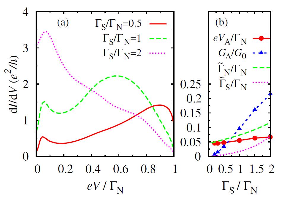
Figure 21: Non-linear conductance for the N-QD-S system using the interpolative self-energy approach of Ref. Yamada et al. (2010). The results correspond to the symmetric case with $\Gamma_{N}=\Delta$ and different values of $\Gamma_{S}$ and $U$. Reprinted figure with permission from Y. Yamada et al., Journal of the Physical Society of Japan 79, 043705, 2010 Yamada et al. (2010). Copyright (2010) by the Physical Society of Japan.

The non-linear case has been analyzed more recently in Ref. Yamada et al. (2010) by extending the interpolative self-energy approach of Ref. Cuevas et al. (2001) to the non-equilibrium case. The authors consider the case $\Delta=\Gamma_{N}$ and $\epsilon_{0}=-U/2$ for different values of $\Gamma_{S}$ and $U$. Their main findings are illustrated in Fig. 21 corresponding to the non-linear conductance for $U=20\Gamma_{N}$. They observe a Kondo peak which is displaced from zero bias, whose height increases with increasing $\Gamma_{S}$ while its position is only weakly modified. When reducing $\Gamma_{S}$ a second peak develops which shift progressively towards the gap edge $eV/\Gamma_{N}=1$.

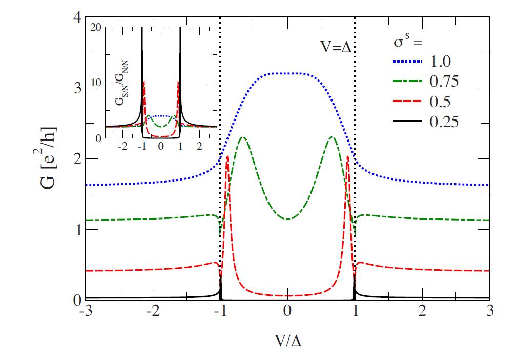
Figure 22: Non-linear conductance for the N-QD-S system in the effective cotunneling model of Ref. Koerting et al. (2010) for even (upper panel) and odd (lower panel) cases. The parameters $\sigma^{e}$ and $\sigma^{s}$ control the normal transmission through the dot in the even and odd cases respectively. The inset shows the differential conductance normalized to the one in the normal case. Reprinted figure with permission from V. Koerting et al., Physical Review B 82, 245108, 2010 Koerting et al. (2010). Copyright (2010) by the American Physical Society.

We should also mention the work of Ref. Koerting et al. (2010) in which the non-equilibrium transport through a N-QD-S system is studied within an effective cotunneling model. Within this approach the self-energy is calculated to leading order in the cotunneling amplitude from which the nonlinear cotunneling conductance can be obtained. By neglecting charge fluctuations in the dot two different regimes are found corresponding to the case of even and odd number of electrons. For the even case the system becomes equivalent to an effective S/N junction with the subgap transport due to Andreev reflection processes. On the other hand, for the odd case they find that the net spin within the dot leads to the appearance of subgap resonances giving rise to a peak-dip structure in the differential conductance. The typical conductance curves that are found for both cases are shown in Fig. 22. As can be observed, in the even case (upper panel in Fig. 22) the behavior of the conductance is similar to a conventional NS junction with an effective transmission set by the second-order cotunneling amplitude. In the odd case (lower panel) the double peak structure within the subgap region evolves into a single zero bias peak as the cotunneling amplitude increases.

To conclude this section it appears that our present knowledge of the non-equilibrium N-QD-S system is still limited and further research would be desirable, particularly to understand the behavior of Kondo features at finite applied voltages and the crossover between the different parameter regimes so far analyzed. In this respect we refer the interested reader to a recent work Yamada et al. (2011) that has been published after submitting this review.

IV.3 Experimental results

Unlike the case of the S-QD-S system, only a few works have addressed the issue of the transport properties of N-QD-S systems experimentally. This is probably due to the technical difficulties associated to the fabrication of such hybrid systems. The first experimental realization of this configuration was presented by Gräber et al. Graber et al. (2004) using a multiwall CNT as a QD coupled to Au (normal) and Al/Au (superconducting) leads at each side. They first analyzed the normal case by applying a magnetic field of $25mT$, clearly observing Kondo features in the linear conductance, as shown in the upper panel of Fig. 23. At the lowest temperature of $90mK$ the normal conductance reached values $\sim 1.5e^{2}/h$, indicating good and rather symmetric coupling to the leads. When one of the leads become superconducting it was observed that the temperature dependence characteristic of the Kondo regime was very much suppressed, as shown in the lower panel of Fig. 23. This behavior is in qualitative agreement with the theoretical results of Refs. Cuevas et al. (2001); Tanaka et al. (2007a) for the case of a nearly symmetrically coupled dot.

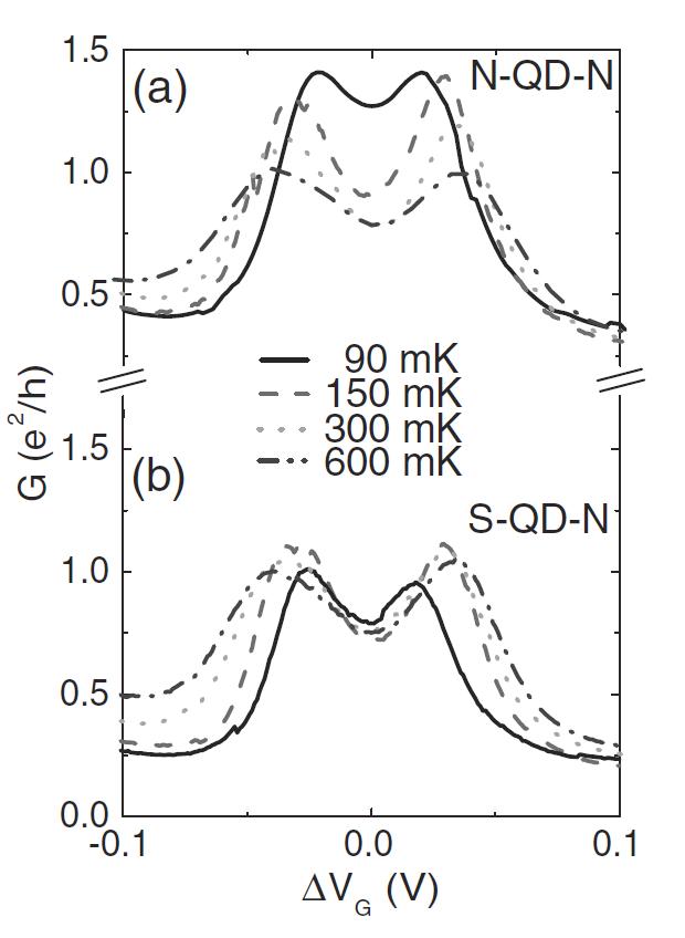
Figure 23: Comparison between the linear conductance in the NQDN and SQDN systems as a function of the gate voltage for different temperatures in the experimental realization of Ref. Graber et al. (2004). Reprinted figure with permission from M.R. Graber et al., Nanotechnology 15, S479, 2004 Graber et al. (2004). Copyright (2004) by IOP Publishing Ltd.

A different experimental realization of the N-QD-S system was presented in Refs. Deacon et al. (2010b, a). These authors used a self-assembled InAs QD with diameters of the order of $\sim 100nm$ coupled to a Ti/Au (N lead) and a Ti/Al (S lead). In the first of these works the authors focused on devices with large coupling asymmetry $\Gamma_{S}\gg\Gamma_{N}$ in which the Kondo effect is suppressed by the strong proximity effect. In this limiting situation the normal lead is basically providing a means to probe spectroscopically the Andreev spectra of the QD-S system. The experiment provided evidence of the transition between the singlet and the doublet ground state for the QD-S system when the number of electrons changed from even to odd. As shown in Fig. 24 this was reflected in the behavior of the Andreev states within the gap exhibiting a crossing point together with a large drop in the conductance. These experimental results were in good qualitative agreement with NRG calculations for the QD-S system.

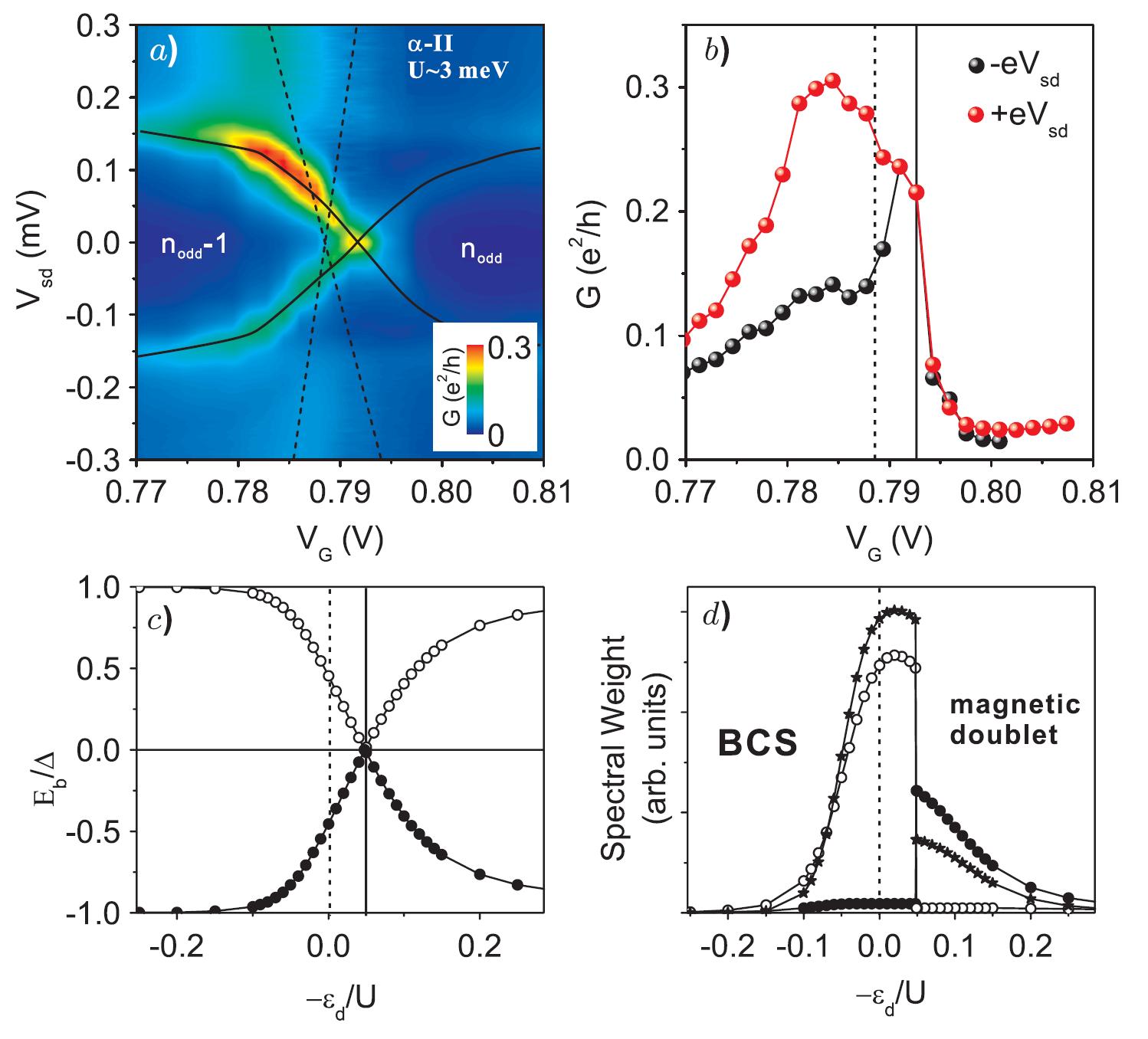
Figure 24: (a) Color scale map of the differential conductance as a function of the source-drain and gate voltages in the experimental realization of the N-QD-S system of Ref. Deacon et al. (2010b). (b) plot of the peak conductance following the subgap resonances indicated by the full lines in (a). Panels (c) and (d) show the Andreev levels position and weight respectively obtained using the NRG method for $U/\Delta=20$ and $\Gamma_{S}/\Delta=0.7$. Reprinted figure with permission from R.S. Deacon et al., Physical Review Letters 104, 076805, 2010 Deacon et al. (2010b). Copyright (2010) by the American Physical Society.

In a subsequent work by this group Deacon et al. (2010a) the same experimental realization but with varying coupling asymmetry was analyzed. The main results of this work are shown in Fig. 25 corresponding to asymmetries $\Gamma_{S}/\Gamma_{N}=0.045$ (upper panel) and $8.0$ (two lower panels). For the first case with sufficiently large $\Gamma_{N}$ one would expect the formation of a Kondo resonance due to the good coupling of the QD with the normal electrode. However, the conductance which is mediated by Andreev processes is suppressed inside the gap due to the very small coupling to the superconductor. The cases with asymmetries of the order of 8.0 were not in the extreme situation of the previous work (with $\Gamma_{S}/\Gamma_{N}\sim 50$) and thus did exhibit Kondo features as can be observed in the lower panels of Figs. 25.

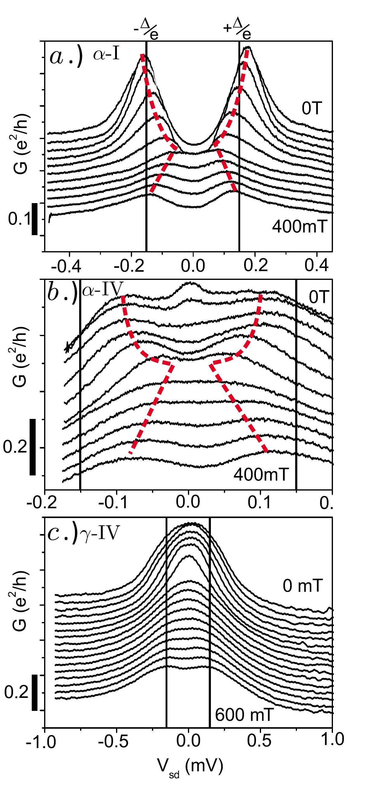
Figure 25: Differential conductance at the center of odd occupation regions for three different samples of the experimental realization of the N-QD-S system of Ref. Deacon et al. (2010a) as a function of the applied magnetic field. The three cases correspond to different values of the $\Gamma_{S}/\Gamma_{N}$ parameter: 0.045 (upper panel) and 8.0 (middle and lower panels). Reprinted figure with permission from R.S. Deacon et al., Physical Review B 81, 121308, 2010 Deacon et al. (2010a). Copyright (2010) by the American Physical Society.

V Voltage biased S-QD-S systems

Including a finite bias voltage between the superconducting electrodes in the S-QD-S system poses an additional difficulty in the theory due to the intrinsic time-dependence of the ac Josephson effect. Even in the non-interacting case the inclusion of MAR processes up to infinite order constitutes a challenging problem which in general requires a numerical analysis.

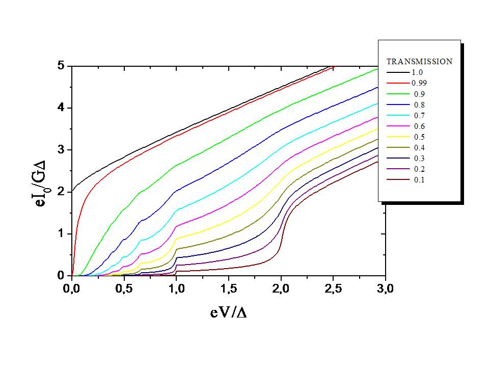
Figure 26: dc I-V characteristic for a superconducting single channel contact for different values of the normal transmission.

Although the mechanism of MAR processes for explaining the subgap structure in superconducting junctions was introduced in the early ’80s Klapwijk et al. (1982); Octavio et al. (1983), it was not until the mid ’90s that a full quantitative theory of the I-V characteristics in a superconducting contact of arbitrary transparency was developed using either a scattering approach Bratus et al. (1995); Averin and Bardas (1995) or a non-equilibrium Green function approach Cuevas et al. (1996). This theoretical progress allowed a very accurate description of experimental results for atomic size contacts Scheer et al. (1998b, a). For the discussion in the present section it could be useful to remind the main features of the I-V characteristics of a one channel contact. Fig. 26 shows the evolution of the dc current as a function of the contact transmission obtained using the theory of Ref. Cuevas et al. (1996). As can be observed, at sufficiently low transmission the current exhibits a subgap structure with jumps at $V=2\Delta/n$, corresponding to the threshold voltage for an $n$-order MAR process. As the transmission is increased the subgap structure is progressively smeared out and eventually at $\tau=1$ the behavior of the I-V curve is almost linear except in the limit $V\rightarrow 0$ where it saturates to a finite value $2e\Delta/h$ Averin and Bardas (1995); Cuevas et al. (1996).

The case of a non-interacting resonant level coupled to superconducting electrodes was first analyzed in Ref. Yeyati et al. (1997). We discuss briefly here the Green function formalism for this case which has the advantage of allowing to include the effect of interactions in a second step. The main point in this formalism is to realize that even when the Green functions $\breve{G}(t,t^{\prime})$ depends on the two time arguments, in the case of a constant voltage bias the dependence on the mean time $(t+t^{\prime})/2$ can only correspond to the harmonics of the fundamental frequency $eV/\hbar$ Cuevas et al. (1996). This allows to express all quantities in terms of the components $\breve{G}_{nm}(\omega)$ corresponding to a double Fourier transformation Arnold (1987) of $\breve{G}(t,t^{\prime})$ defined as Martín-Rodero et al. (1999a)

$$\breve{G}_{nm}(\omega)=\int dt\int dt^{\prime}e^{-iV(nt-mt^{\prime})}e^{i\omega(t-t^{\prime})}\breve{G}(t,t^{\prime})$$ (35)

The Fourier components $\breve{G}_{nm}$ obey an algebraic Dyson equation in the discrete space defined by the harmonic indices which can be solved using a standard recursive algorithm. A compact expression of these equations for the dot case, given in Ref. Dell’Anna et al. (2008), is

$$(\breve{G_{00}})^{-1}_{nm}=\left(\omega_{n}-\epsilon_{0}\sigma_{z}\right)\tau_{z}-\sum_{\mu=L,R}\Gamma_{\mu}\sigma_{z}\tau_{z}\breve{g}_{nm}(\omega)\sigma_{z}\tau_{z}$$ (36)

where $\omega_{n}=\omega+nV$, while $\sigma_{i}$ and $\tau_{i}$ correspond to Pauli matrices in the Nambu and Keldysh space respectively and

$$\breve{g}_{nm}=\left(\begin{array}[]{cc}\delta_{nm}\breve{X}(\omega_{n}\mp V/2)&\delta_{n,m\mp 1}\breve{Y}(\omega_{n}\mp V/2)\\ \delta_{n,m\pm 1}\breve{Y}(\omega_{n}\pm V/2)&\delta_{nm}\breve{X}(\omega_{n}\pm V/2)\end{array}\right)$$ (37)

where the matrix $\breve{X}(\omega)=-\omega\breve{Y}/\Delta$ in Keldysh space are given by

$$\breve{X}(\omega)=\left\{\begin{array}[]{lr}-\frac{\omega}{\sqrt{\omega^{2}-\Delta^{2}}}\tau_{z}&|\omega|>\Delta\\ \frac{i|\omega|}{\sqrt{\Delta^{2}-\omega^{2}}}\left(\begin{array}[]{cc}2n_{F}(\omega)-1&2n_{F}(\omega)\\ 2n_{F}(-\omega)&2n_{F}(\omega)-1\end{array}\right)&|\omega|<\Delta\end{array}\right.$$ (38)

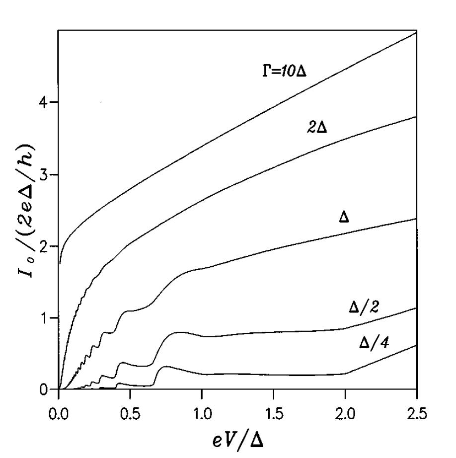
Figure 27: dc I-V characteristic for the non-interacting S-QD-S system with $\epsilon_{0}=0$ and different values of $\Gamma=\Gamma_{L}=\Gamma_{R}$. Reprinted figure with permission from A. Levy Yeyati et al., Physical Review B 55, 6137, 1997 Yeyati et al. (1997). Copyright (1997) by the American Physical Society.

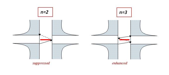
Figure 28: Schematic representation of MAR processes of order $n=2$ and $n=3$. The central horizontal line represents the level position, assumed to be located at the Fermi level.

The presence of a discrete resonant level between the superconducting leads can strongly modify the I-V characteristics with respect to the quantum point contact case. This is illustrated in Fig. 27 which corresponds to a resonant level located at zero energy with decreasing tunneling rates to the leads. As the figure shows, in the limit of large $\Gamma$ the I-V curves tend to that of a perfect transmitting contact. In the opposite limit $\Gamma\ll\Delta$ there appears a pronounced subgap structure. In contrast to the contact case, the current jumps associated to the threshold of MAR processes appear only for the condition $V=2\Delta/n$ with $n$ being an odd integer, while the features at $2e\Delta/n$ with even $n$ are suppressed. This can be understood qualitatively from the schematic pictures of Fig. 28. They represent the $n=2$ and $n=3$ MAR processes with arrows indicating propagation of electrons (full lines) or holes (broken lines). In the $n=2$ case the MAR “trajectory” in energy space does not cross the resonant level while in the $n=3$ case the resonant condition is fulfilled.

Figure 29: dc I-V characteristic for the non-interacting S-QD-S system with $\Gamma_{L}=\Gamma_{R}=\Delta$ and different dot level positions: 5 (a), 2 (b), 1 (c), 0.5 (d) and 0 (e) in units of $\Delta$. Reprinted figure with permission from A. Martín-Rodero et al., Superlattices and Microstructures 25, 925, 1999 Martín-Rodero et al. (1999b). Copyright (1999) by Elsevier.

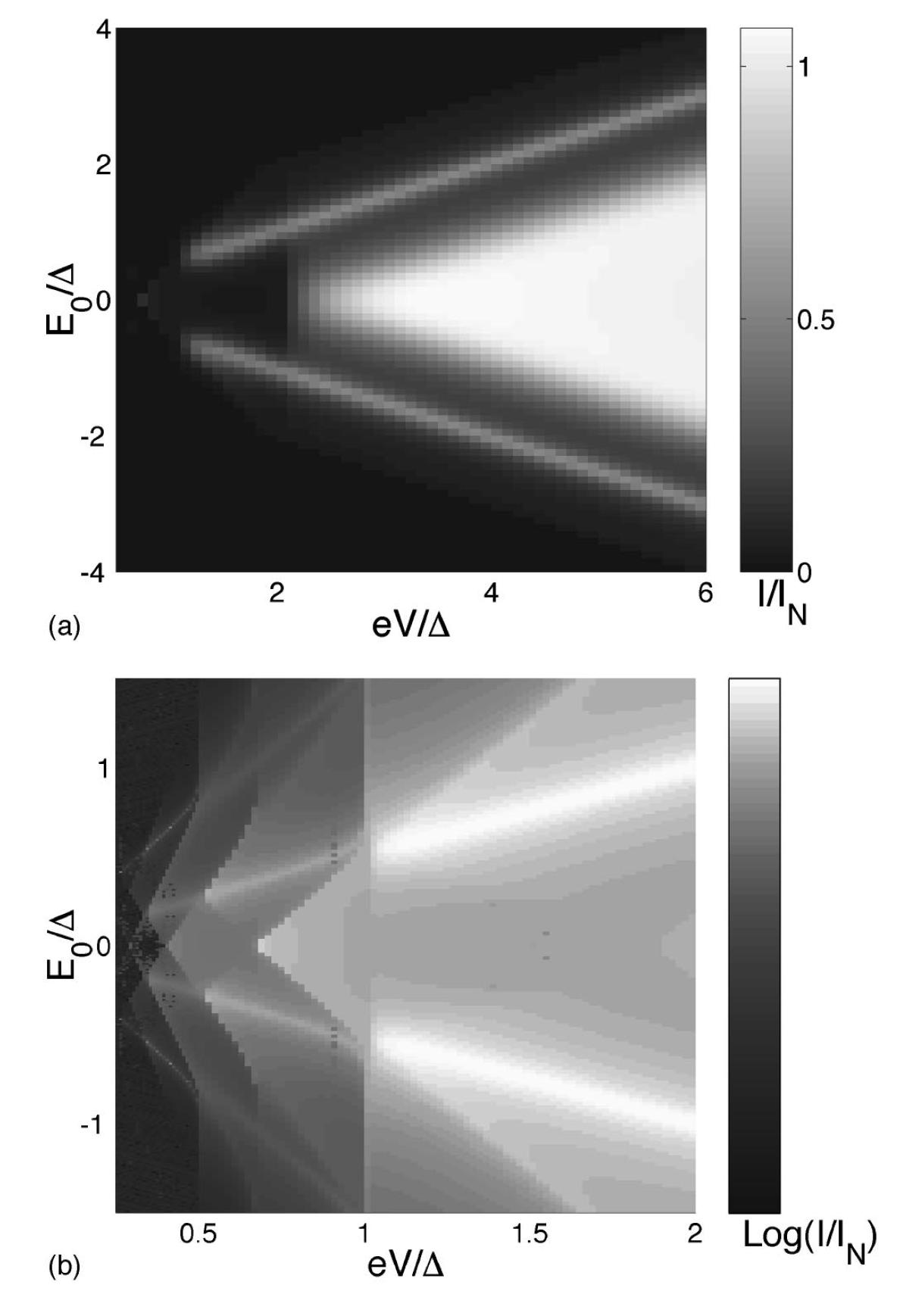
Figure 30: Color scale map of the the dc current in the $\epsilon_{0}$-$eV$ plane for the non-interacting S-QD-S system. The upper panel corresponds to $eV>\Delta$ and $\Gamma=0.2\Delta$ while the lower panel corresponds to $eV<2\Delta$ and $\Gamma=0.05\Delta$. Reprinted figure with permission from G. Johansson et al., Physical Review B 60, 1382, 1999 Johansson et al. (1999). Copyright (1999) by the American Physical Society.

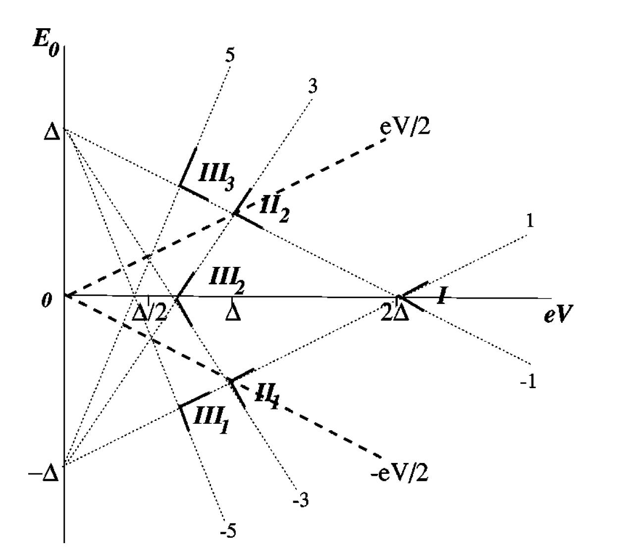
Figure 31: Lines indicating the boundaries for the resonant regions of the single, double and triple quasiparticle currents in the $\epsilon_{0}$-$eV$ plane for the non-interacting S-QD-S system. Reprinted figure with permission from G. Johansson et al., Physical Review B 60, 1382, 1999 Johansson et al. (1999). Copyright (1999) by the American Physical Society.

The subgap features are quite sensitive to the level position. Fig. 29 illustrates the evolution of the I-V characteristics as a function of the level position $\epsilon_{0}$ for the case $\Gamma_{L}=\Gamma_{R}=\Delta$. As can be observed, when the level is far from the gap region the behavior of a weakly transmitting contact is recovered, while in the case where the level approaches the gap, the subgap features become more pronounced and correspond to resonant conditions which depend both on $\Delta$ and $\epsilon_{0}$. In this complex situation a more clear picture of the overall behavior was presented in Ref. Johansson et al. (1999). Figs. 30 show the intensity plot of the current in the $\epsilon_{0}-V$ plane. The upper panel illustrates the behavior of the current for $eV>\Delta$ for $\Gamma=0.2\Delta$, showing clearly the onset of single quasiparticle current for $eV>2\Delta$ at $\epsilon_{0}=0$. For $\epsilon_{0}\neq 0$ this current is only significant in a wedge-like zone limited by $\epsilon_{0}=\pm(V-2\Delta)/2$. It can also be noticed in addition the presence of resonant peaks at $V/2=\pm\epsilon_{0}$ which are reminiscent of the resonant condition for the normal case. The lower panel shows the intensity map in the region $eV<2\Delta$ for $\Gamma=0.05\Delta$. This illustrates the onset of higher order MAR processes, which also appear to be limited into wedge-like regions bounded by the condition $\epsilon_{0}=\pm(\Delta-neV/2)$ with odd $n$. The schematic figure 31 indicates the different resonant regions for the single, double and triple quasi-particle currents.

In subsequent works further analysis of the non-interacting S-QD-S case out of equilibrium was presented Sun et al. (2002); Jonckheere et al. (2009a). While in Ref. Sun et al. (2002) the Hamiltonian approach was used to analyze the out of equilibrium dot spectral density and the ac components of the current, in Ref. Jonckheere et al. (2009a) the effect of dephasing simulated by a third normal reservoir coupled to the dot has been studied. This work will be further commented in Sect. VI.

V.1 Effect of Coulomb interactions

The inclusion of intradot interactions in the out of equilibrium S-QD-S system introduces an additional difficulty in an already challenging theoretical problem, as shown in the previous section. So far the attempts have been restricted to some limiting cases which have been treated using approximate methods. One of these special limiting situations which was first analyzed was the case of a quantum dot in the strong Coulomb blockade regime Whan and Orlando (1996); Yeyati et al. (1997). These works were motivated by the experimental results of Ref. Ralph et al. (1995) for transport through small metallic nanoparticles coupled to superconducting leads. In this strong blockade regime multiple quasiparticle processes are suppressed and the current is basically due to single quasiparticle tunneling.

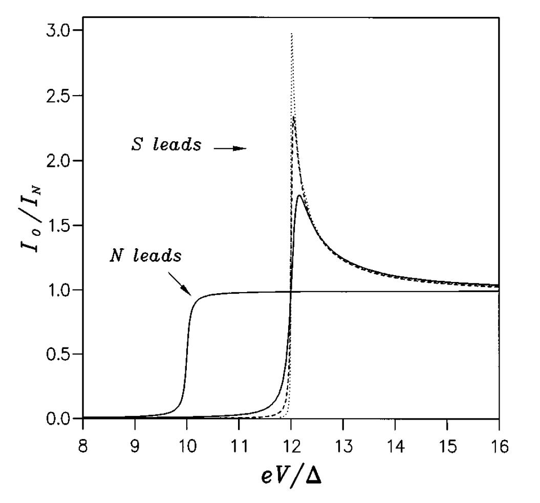
Figure 32: dc current-voltage characteristic for a S-QD-S system in the strong Coulomb blockade regime for different values of $\Gamma_{L}=$ $5\times 10^{-3}\Delta$ (full line), $10^{-3}\Delta$ (dashed line) and $2\times 10^{-4}\Delta$ (dotted line), with $\epsilon=5\Delta$. Reprinted figure with permission from A. Levy Yeyati et al., Physical Review B 55, 6137, 1997 Yeyati et al. (1997). Copyright (1997) by the American Physical Society.

In Ref. Whan and Orlando (1996) the current was calculated in this regime by means of a master equation approach assuming a sequential tunneling regime. The single-particle tunneling rates were calculated using the Fermi golden-rule. A slightly different method was used in Ref. Yeyati et al. (1997) where resonant tunneling through an effective one-electron level describing the dot in the limit $U\rightarrow\infty$ was considered. The corresponding expression for the tunneling current was given by

$$I(V) = \frac{4e}{h}\int d\omega\frac{\Gamma_{L}(\omega)\Gamma_{R}(\omega)}{(\omega-\epsilon)^{2}+\left[\Gamma_{L}(\omega)+\Gamma_{R}(\omega)\right]^{2}}$$ (39)

$$\times\left[n_{F}(\omega-eV/2)-n_{F}(\omega+eV/2)\right],$$

where $\epsilon$ denotes the effective level and

$$\Gamma_{L,R}(\omega)=(\Gamma/2)\mbox{Re}\left[|\omega\pm V/2|/\sqrt{(\omega\pm V/2)^{2}-\Delta^{2}}\right].$$

The corresponding result for different values of $\Gamma$ are shown in Fig. 32. This result differs from the simple sequential tunneling picture, which would predict $I(V)\sim\Gamma_{L}(\epsilon)\Gamma_{R}(\epsilon)/(\Gamma_{L}(\epsilon)+\Gamma_{R}(\epsilon))$, exhibiting an intrinsic broadening of the BCS-like feature, in agreement with the experimental observation Ralph et al. (1995). A similar expression was obtained in Ref. Kang (1998) using the equation of motion approach in the atomic limit which produces a correction factor in the current, $\sim\sum_{\sigma}(1-<n_{0\sigma}>)$ due to the strong Coulomb interaction.

In order to analyze the interplay of MAR and Kondo correlations it is necessary to rely on other approaches. In Ref. Avishai et al. (2003) the current-voltage of this system was obtained using the slave boson mean field approximation already discussed in Sect. III. In the infinite-U version of the method used in Ref. Avishai et al. (2003) the problem becomes equivalent to an effective non-interacting model with renormalized parameters $\tilde{\Gamma}$ and $\tilde{\epsilon}_{0}$, as indicated in subsection III.2. The authors analyze the evolution of the I-V curves and the shot-noise as a function of the parameter $T_{K}/\Delta$. As is physically expected, the behavior is similar to that of a perfectly transparent contact when $T_{K}/\Delta\gg 1$ developing a clear subgap structure in the opposite limit.

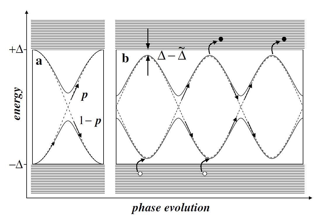
Figure 33: Schematic representation of the ABS dynamics explaining the low bias dc current in the case of a single channel contact (panel a) and for the S-QD-S system in the Kondo regime (panel b). Reprinted figure with permission from A. Levy Yeyati et al., Physical Review Letters 91, 266802, 2003 Yeyati et al. (2003). Copyright (2003) by the American Physical Society.

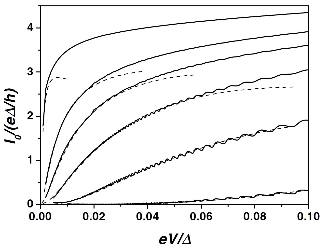
Figure 34: Comparison of the low bias dc current in the S-QD-S system in the Kondo regime obtained from the ABS dynamics (dashed lines) and by the full numerical calculation (full line) for different values of the effective coupling to the leads $\tilde{\Gamma}_{L}=\tilde{\Gamma}_{R}=1,2,3,4,5$ and $10$ in units of $\Delta$, from bottom to top. Reprinted figure with permission from A. Levy Yeyati et al., Physical Review Letters 91, 266802, 2003 Yeyati et al. (2003). Copyright (2003) by the American Physical Society.

A similar approach was used in Ref. Yeyati et al. (2003) in order to analyze the low bias transport properties of a S-QD-S in the Kondo regime $T_{K}\gg\Delta$. It was shown that these properties can be understood in terms of the dynamics of the subgap Andreev states. In this limit the ABSs satisfy the equation corresponding to the non-interacting case, ie. Eq. (12), with renormalized parameters $\tilde{\Gamma}_{L,R}$ and $\tilde{\epsilon}_{0}$ instead of $\Gamma_{L,R}$ and $\epsilon_{0}$. The low bias quasiparticle current through the system arises from transitions between the continuum occupied and empty states below and above the superconducting gap which occur by means of Landau-Zener like processes involving the ABSs. This is illustrated in Fig. 33 first for the case of a quantum point contact (left panel) and then for the S-QD-S case (right panel). In the last case it is necessary to have a transition between the ABSs and the continuum in addition to the Landau-Zener transition between the lower and upper ABSs. The results for the low bias dc current which are obtain from this analysis, shown in Fig. 34, are in good agreement with the results of a full numerical calculation including MAR processes up to infinite order. The analysis based on the dynamics of the ABSs was also used in Ref. Vecino et al. (2004) for a comparison of experimental results in the low bias regime. In contrast to Ref. Yeyati et al. (2003), in this work a phenomenological damping rate $\eta$ was introduced in order to fit the experimental data obtained for multiwall CNTs connected to Au/Al leads.

A step beyond the infinite-$U$ SBMF approach was taken in Ref. Eichler et al. (2007) where the finite-U SBMF method was used to determine the I-V characteristics of a S-QD-S system. This approach allowed to describe the observed differences in the subgap structure between situations with even and odd number of electrons in the dot for a SWCNT QD coupled to Al/Ti electrodes. In Ref. Eichler et al. (2007) the effective parameters of the finite-U SBMF approach were obtained for the leads in the normal state and assumed to remain unmodified in the superconducting case. The results of this work for the subgap structure are shown in Fig. 35 where the comparison with the experimental data is given. The figure corresponds to an odd valley exhibiting clear Kondo features in the normal state. The more intriguing feature of the differential conductance in the superconducting case was the presence of a pronounced structure for $eV\sim\Delta$, which cannot be explained by the non-interacting theory. This feature was attributed to the large asymmetry $\Gamma_{L}/\Gamma_{R}\sim 30$ which produces a Kondo resonance pinned at the chemical potential of the left lead. As is schematically depicted in Fig. 35(e) this resonance would produce and enhancement of the current for $eV\sim\Delta$.

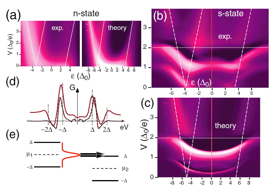
Figure 35: Experimental and theoretical results for the differential conductance of the S-QD-S system in an odd valley. Panel (a) corresponds to the normal state (experimental and theoretical results), while (b) and (c) show the corresponding results in the superconducting state. Panel (d) shows the conductance vs voltage bias along the line indicated in red in panels (b) and (c). The theoretical curves corresponds to $\Gamma_{L}=\Delta$, $\Gamma_{R}=0.03\Delta$ and $U=10\Delta$. Reprinted figure with permission from A. Eichler et al., Physical Review Letters 99, 126602, 2007 Eichler et al. (2007). Copyright (2007) by the American Physical Society.

The effect of interactions in the subgap structure has also been considered in Ref. Dell’Anna et al. (2008) by means of a perturbative approach in which the dot self-energy was calculated up to second order in $U$. The method thus includes the diagrams already discussed in Sect. III but extended to the non-equilibrium situation. To avoid heavily time-consuming computation of the multiple frequency integrals, the authors calculate the diagrams in time representation and then Fourier transform the final result. They consider the weak interaction regime $U/\Gamma<1$ thus avoiding the regime of $\pi$-junction behavior. The most remarkable result is the observation of an enhancement of the current due to the interactions, which is more pronounced for voltages approaching the odd MAR onset conditions $2\Delta/(2r+1)$. This is illustrated in Fig. 36 for the case $\epsilon_{0}=0$ where the difference $I(U)-I(0)$ as a function of $2\Delta/V$ is represented. The enhancement is observed both in the self-consistent first order approximation and when including the second-order diagrams. This current enhancement is reminiscent yet different from the “antiblockade” behavior due to dynamical Coulomb blockade effects on MAR transport, as discussed in Ref. Yeyati et al. (2005). It is worth mentioning that MAR transport through a resonant level coupled to a localized phonon mode was studied in Ref. Zazunov et al. (2006) using second order perturbation theory in the electron-phonon coupling.

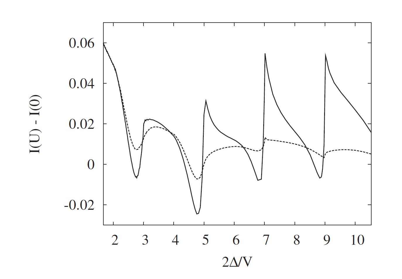
Figure 36: Variation of the dc current in the symmetric S-QD-S system with respect to the non-interacting case obtained in Ref. Dell’Anna et al. (2008) using the second-order self-energy approach for $U/\Gamma=\Gamma/\Delta=0.5$. The dashed curve gives the self-consistent first order result. Reprinted figure with permission from L. Dell’Anna et al., Physical Review B 77, 104525, 2008 Dell’Anna et al. (2008). Copyright (2008) by the American Physical Society.

V.2 Summary of Experimental results

The already commented work by Ralph et al. Ralph et al. (1995) can be considered one of the first realizations of a S-QD-S system in which the current-voltage characteristic was measured. This case corresponded, however, to the strong blockade regime in which the subgap structure is absent. It was not until 2002 that experiments on CNTs coupled to Al leads Buitelaar et al. (2002, 2003) allowed a clear observation of the subgap features. Ref. Buitelaar et al. (2002) mainly focused in the linear conductance which can exhibit either an enhancement or a suppression with respect to the normal case depending on the ratio $T_{K}/\Delta$. The results of this work are summarized in Fig. 37. On the other hand in Ref. Buitelaar et al. (2003) the authors analyzed the MAR induced subgap structure for the same type of systems in more detail. As shown in Fig. 38 clear peaks in the differential conductance are observed at the positions $eV\sim 2\Delta$, $\Delta$ and $\Delta/2$. The intensity of these peaks evolves as a function of the dot level position (controlled by the gate voltage $V_{g}$). Contrary to the theoretical expectations the peak at $\Delta$ is still visible at resonance whereas the expected feature from the non-interacting model at $2\Delta/3$ is not observed. The authors of Ref. Buitelaar et al. (2003) suggest that the discrepancy can be attributed to the effect of interactions not included in their theoretical analysis. These results could be analyzed in the light of the already commented arguments of Ref. Eichler et al. (2007) which attributed the pronounced $\Delta$ peak to the combined effect of coupling asymmetry and Kondo effect.

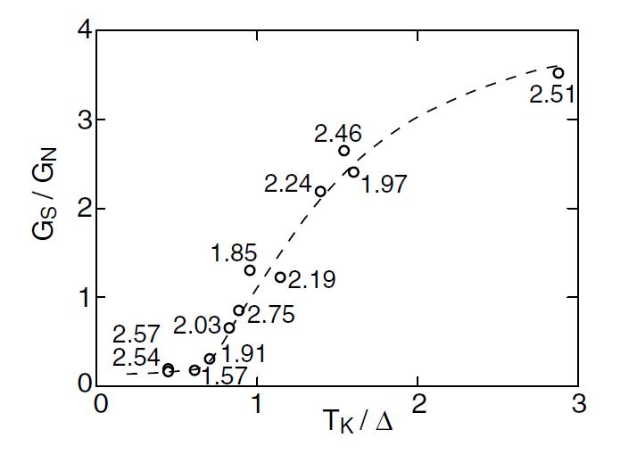
Figure 37: Linear conductance in the Kondo regime for the experimental realization of the S-QD-S system of Ref. Buitelaar et al. (2002) normalized to its value in normal state as a function of $T_{K}/\Delta$. Reprinted figure with permission from M.R. Buitelaar et al., Physical Review Letters 89, 256801, 2002 Buitelaar et al. (2002). Copyright (2002) by the American Physical Society.

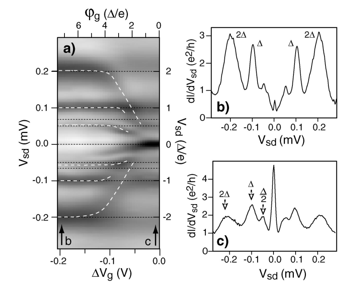
Figure 38: Results for the differential conductance in the experimental realization of the S-QD-S system of Ref. Buitelaar et al. (2003). Panel (a) color map for this quantity in the bias voltage-gate voltage plane. The dashed lines indicate the evolution of the MAR resonances. Panels (b) and (c) show plot of the conductance as a function of bias for the lines indicated by the arrows in panel (a). Reprinted figure with permission from M.R. Buitelaar et al., Physical Review Letters 91, 057005, 2003 Buitelaar et al. (2002). Copyright (2003) by the American Physical Society.

The competition between Kondo effect and superconductivity was also observed in Ref. Buizert et al. (2007) in which self-assembled InAs quantum dots contacted with Al leads were analyzed. A magnetic field was used to control the size of the superconducting gap parameter and the linear conductance as a function of $\Delta/k_{B}T_{K}$ was measured. The results exhibited a rather universal behavior as a function of this parameter. However, in contrast to Ref. Buitelaar et al. (2002) the ratio $G_{S}/G_{N}$ did not exceed unity for $\Delta/k_{B}T_{K}<1$ while decreasing as expected for $\Delta/k_{B}T_{K}>1$. Although the authors attributed this difference to a stronger Coulomb repulsion which would in their case heavily damp the MAR processes, one would expect that this effect would be already included when scaling $\Delta$ in units of $T_{K}$. The absence of conductance enhancement for large $T_{K}$ could be also pointing out to an ingredient in this system not included in the simplest Anderson model like spin-orbit interactions.

VI Beyond the single level model: multidot, multilevel and multiterminal systems

In recent years there has been an increasing interest in more complex situations which cannot be described by the simplest single level Anderson model. These include situations where transport occurs through more than a single dot or where several quantum channels in a single dot are involved. In addition, there is also great interest in analyzing the transport properties of hybrid quantum dot systems coupled to several superconducting and/or normal electrodes in a multiterminal configuration. These configurations could allow to explore non-local electronic transport, in particular the possibility of creating entangled electron pairs by means of crossed or non-local Andreev processes. To describe these developments we organize this section as follows: in the first subsection we discuss the case of Josephson transport through double and multiple dot systems, in the second one we consider this effect for a multilevel dot, and finally we consider multiple dot systems including both normal and superconducting electrodes as well as in a multiterminal configuration.

VI.1 Josephson effect through multidot systems

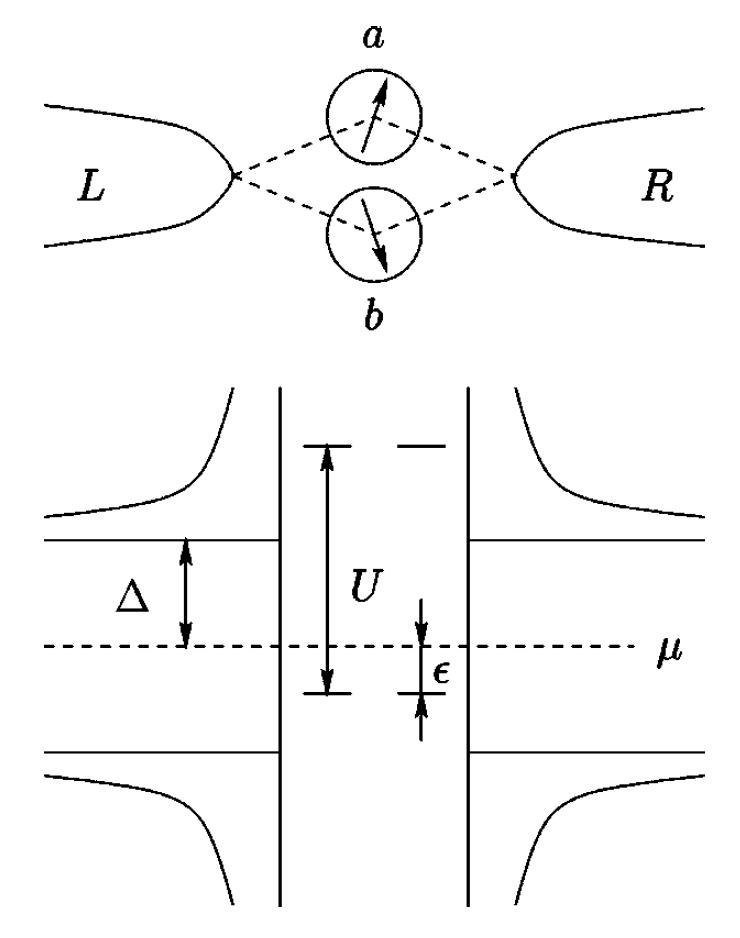
Figure 39: Schematic representation of a double dot system coupled in parallel to two superconducting electrodes (upper panel) considered in Ref. Choi et al. (2000). The lower panel describe the leads spectral density and the parameters of the double dot Anderson model used in this reference. Reprinted figure with permission from M.S. Choi et al., Physical Review B 62, 13569, 2000 Choi et al. (2000). Copyright (2000) by the American Physical Society.

Transport through double quantum dots connected either in parallel or in series to superconducting electrodes has been extensively analyzed in the literature. Most of the theoretical works describe this situation by using a single-level Anderson model to represent each dot and introducing extra terms describing the coupling to the leads. Choi et al. considered in Ref. Choi et al. (2000) the case of two dots connected in parallel to superconducting leads as depicted in Fig. 39. By analyzing the problem to the fourth order in the tunneling to the leads they derived an effective Hamiltonian coupling the localized spins in both dots. In the regime $0<-\epsilon_{0}<<\Delta<<U$ this Hamiltonian adopts the form

$$H_{eff}\simeq J\left(1+\cos{\varphi}\right)\left[{\bf S}_{a}.{\bf S}_{b}-\frac{1}{4}\right],$$ (40)

where $J$ is an exchange coupling between the localized spins in dots $a$ and $b$; and $\varphi$ is defined as

$$\varphi=\phi_{L}-\phi_{R}-\frac{\pi}{\Phi_{0}}\int\left(dl_{a}+dl_{b}\right).{\bf A},$$ (41)

where the last term corresponds to the phase accumulated on each path of the loop due to the magnetic field. These results indicate that the Josephson current through such a device would be sensitive to the total spin of the double dot. In order to probe the spin state of the double dot system the authors propose to incorporate it into a SQUID geometry in which an additional tunnel junction is included in one of its arms. Further elaboration on similar ideas were presented in Ref. Hur et al. (2006) for a triple dot between superconducting leads. This system is shown to behave under certain conditions as a mesoscopic pendulum where the singlets injected through a pair of dots oscillate between two different configurations like in the resonating valence bond model.

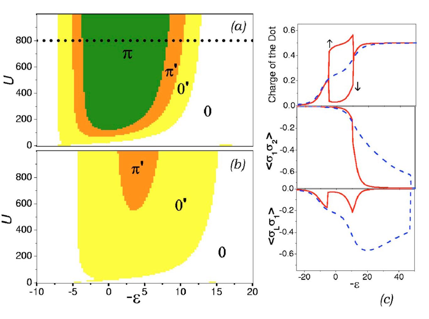
Figure 40: $U-\epsilon$ phase diagrams, dot population and spin correlation functions for the series double dot model considered in Ref. Bergeret et al. (2006) obtained using the zero band-width approximation to describe the superconducting leads. The parameters are $t_{12}=10\Delta$, $t_{L}=t_{R}=2\Delta$ (a) and $t_{L}=t_{R}=2.5\Delta$ (b). The plots in panel (c) are taken along the dotted line corresponding to $U=800\Delta$ shown in panel (a). Reprinted figure with permission from F.S. Bergeret et al., Physical Review B 74, 132505, 2006 Bergeret et al. (2006). Copyright (2006) by the American Physical Society.

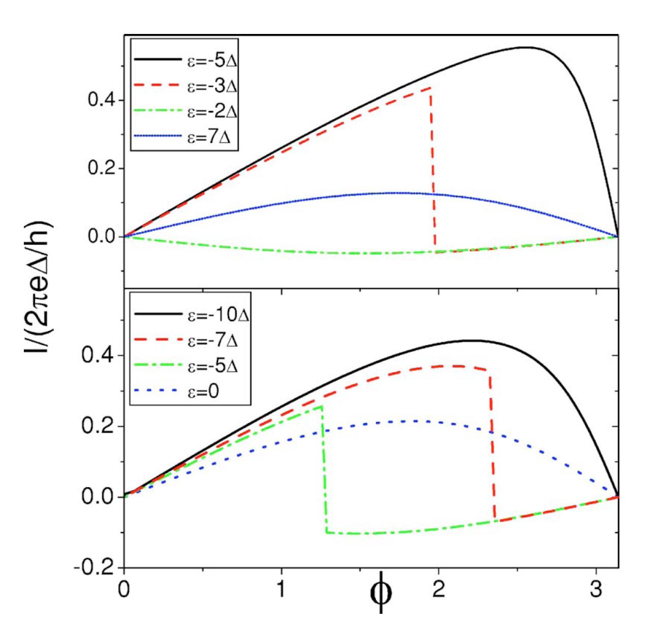
Figure 41: Current-phase relation for the model considered in Ref. Bergeret et al. (2006) obtained using the finite-U SBMF method with parameters $U=800\Delta$, $t_{12}=10\Delta$, $\Gamma_{L}=\Gamma_{R}=2.25\Delta$ (upper panel) and $\Gamma_{L}=\Gamma_{R}=4\Delta$ (lower panel). Reprinted figure with permission from F.S. Bergeret et al., Physical Review B 74, 132505, 2006 Bergeret et al. (2006). Copyright (2006) by the American Physical Society.

The case of two QDs in series connected to superconducting leads was first analyzed in Ref. Zhu et al. (2002). The authors start by diagonalizing exactly the isolated double dot Hamiltonian including a term describing the interdot repulsion $V$ and then introducing the external leads by a Dyson-type equation. This approach should be valid in the limit of vanishing coupling to the leads and is equivalent to the one commented in Sect. III for the single dot case. For the case $U>V>t$, where $t$ is the interdot hopping parameter, and for $k_{B}T\gg\Gamma$ they find that the system exhibits a 0 type current-phase relation except when a finite Zeeman splitting is included. The absence of a $\pi$-junction behavior for any dot filling is probably due to the extremely small value of $\Gamma$ compared to $k_{B}T$. This will be further discussed below.

A similar situation was later considered in Ref. Bergeret et al. (2006), where a double dot model was analyzed using both small cluster numerical diagonalizations (discussed before in Subsect. III.4 for the single dot case) together with the finite-U SBMF technique. In addition to the transition to the $\pi$-phase this work aimed to investigate the interplay between different possible magnetic correlations including Kondo and anti-ferromagnetic coupling between the localized spins within each dot. Part of the results are shown in Fig. 40 where the phase-diagram in the $U$ vs $-\epsilon$ plane is given for the case $t_{12}\gg\Delta$, $t_{12}$ being the interdot hopping parameter. In the range of parameters of Fig. 40 the system exhibits a $\pi$-phase region associated to the transition between the empty and singly occupied double dot. When increasing the dot population to the level of one electron per dot antiferromagnetic correlations dominate and the $\pi$-phase is no longer stable. This is further illustrated in panel (c) of Fig. 40 where different spin-spin correlation functions are shown both for the normal and the superconducting case. The results obtained using the small cluster diagonalizations were confirmed by the finite-U SBMF calculations. In particular these last calculations also show the gradual disappearance of the full $\pi$-phase when increasing the coupling to the leads, as illustrated in Fig. 41. This work also provided a possible scenario for explaining the experimental results of Ref. Kasumov et al. (2005) for fullerene dimers containing Gd magnetic atoms and suggested the possibility to control the magnetic configuration of these atoms by means of the Josephson current.

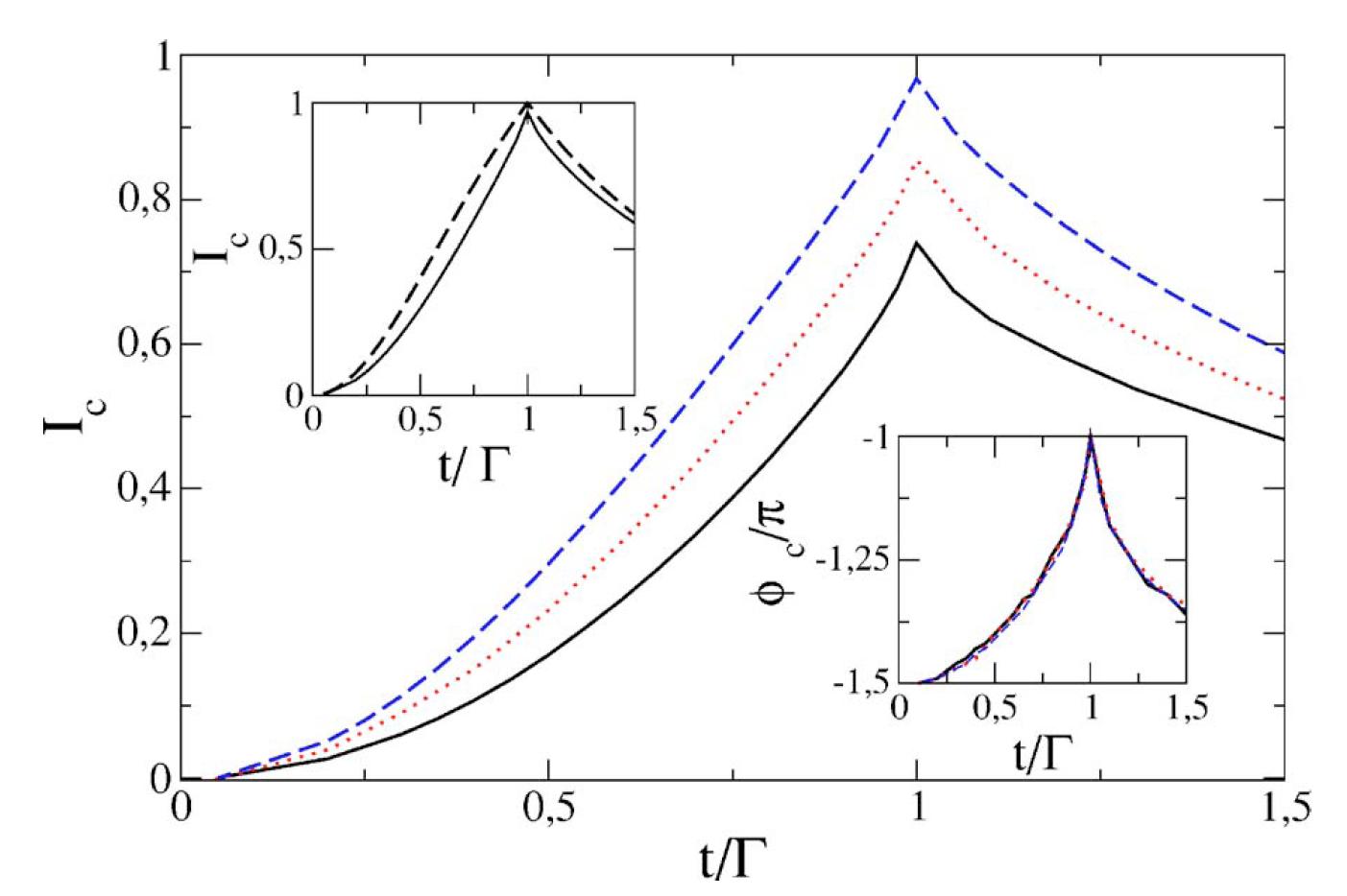
Figure 42: Josephson critical current as a function of $t/\Gamma$ for the series double dot model analyzed in Ref. López et al. (2007) using the infinite-U SBMF method for $\Delta/T_{K}=0.1,0.25$ and 0.5 (from bottom to top). The upper inset shows the comparison of the numerical result for $\Delta/T_{K}=0.1$ (full line) with the prediction from a non-interacting model with an effective transmission (dashed line). The lower inset shows the critical phase at which the maximum current occurs. Reprinted figure with permission from R. López et al., Physical Review B 75, 045132, 2007 López et al. (2007). Copyright (2007) by the American Physical Society.

The SBMF approach in the infinite-U version was applied to series and parallel double quantum dots in Ref. López et al. (2007). As in the case of a single QD this method cannot account for the appearance of a $\pi$-junction phase. The results are nevertheless relevant for the regime $T_{K}\gg\Delta$ where Kondo correlations dominate over pairing. While in the parallel case it is found that the Josephson critical current, $I_{c}$, decreases monotonically with the interdot hopping parameter $t$, in the series case a non-monotonous behavior is found. This is illustrated in Fig. 42 where $I_{c}$ exhibits a maximum at $t/\Gamma\sim 1$. The authors interpret the change in behavior of $I_{c}$ as a transition from a regime characterized by two independent Kondo singlets involving each dot and the corresponding lead to the formation of bonding and antibonding Kondo resonances.

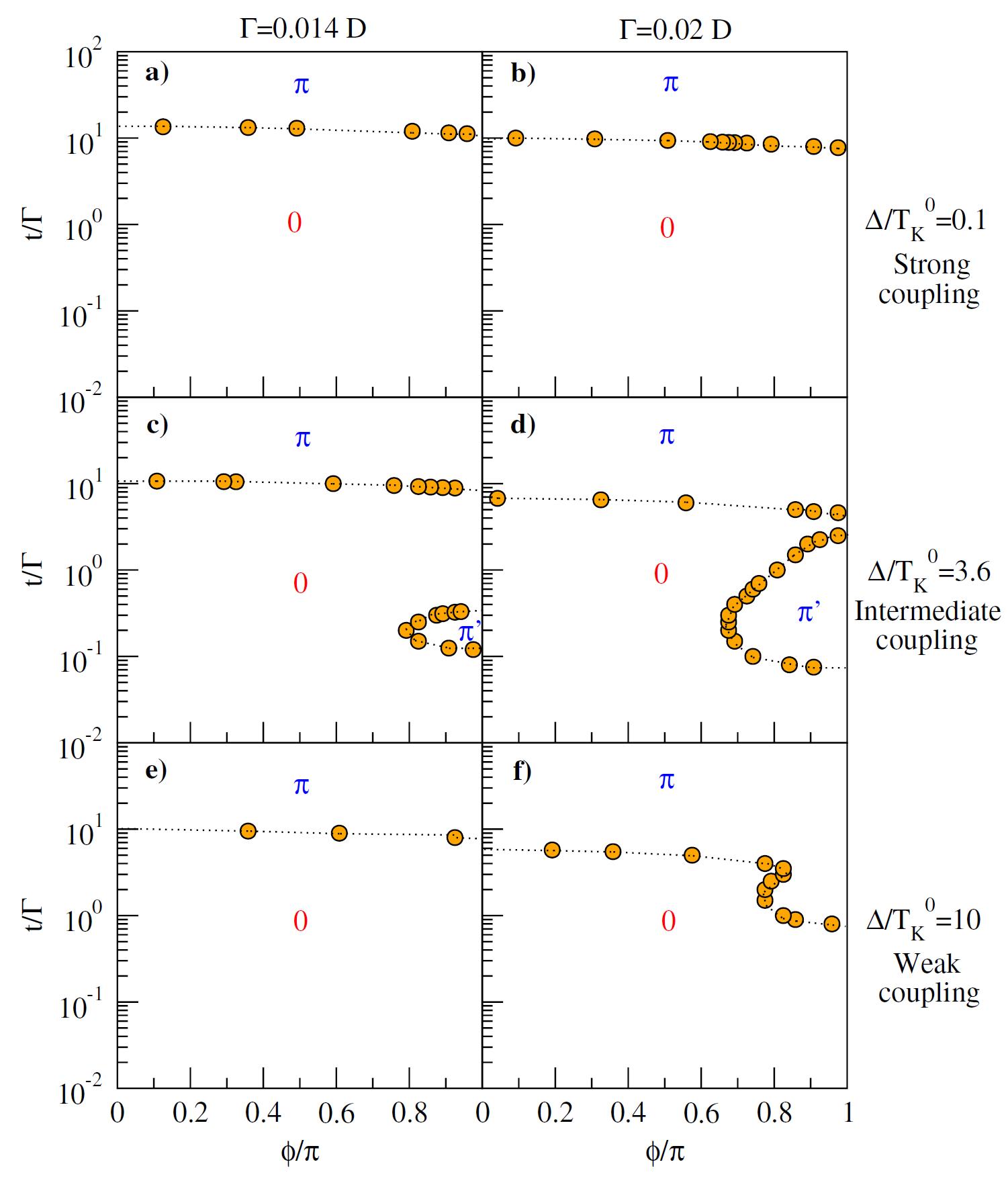
Figure 43: Phase boundaries between the 0 and $\pi$ states in the series double dot model of Ref. Zitko et al. (2010) obtained using the NRG method for $\Gamma=0.014D$ and $\Gamma=0.02D$, where $D$ is the leads band-width. Reprinted figure with permission from R. Zitko et al., Physical Review Letters 105, 116803, 2010 Zitko et al. (2010). Copyright (2010) by the American Physical Society.

Quite recently, the series double dot system coupled to SC leads has been analyzed using the NRG method Zitko et al. (2010). The authors considered the regime $U\rightarrow\infty$ and $-\epsilon\gg\Gamma$, which would correspond to the deep Kondo regime in a normal single QD. In this range of parameters they find a rich phase diagram as a function of the interdot coupling $t$ and the ratio $T_{K}/\Delta$. Some of their results are illustrated in Fig. 43 showing the regions corresponding to $0$, $\pi$ and $\pi^{\prime}$ phases in the $t/\Gamma$ vs $\phi$ plane for different values of $T_{K}/\Delta$. One can notice the abrupt transition between $0$ and $\pi$ phases for $t\sim 10\Gamma$ which can be associated to a change in the DQD population from an even to an odd number of electrons. An additional remarkable feature is the appearance of a $\pi^{\prime}$ ”island” close to $\phi=\pi$ and for $t\sim\Gamma$ in the intermediate coupling regime $T_{K}\sim\Delta$.

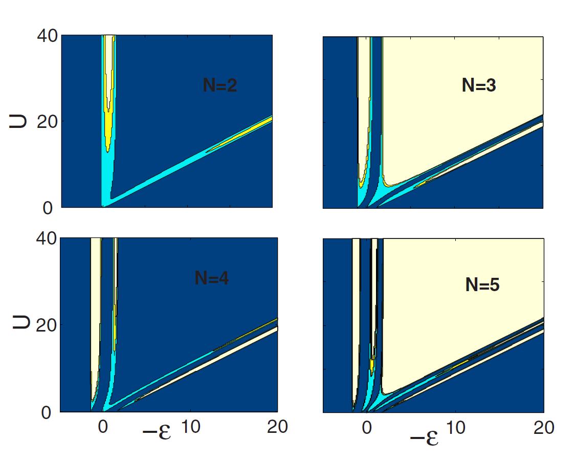
Figure 44: $\epsilon-U$ phase diagrams for the quantum dot array coupled to superconductors considered in Ref. Bergeret et al. (2007) with increasing number of dots $N=2,3,4$ and 5. The results were obtained using the zero band-width approximation described in Subsect. III.4 with parameters $t_{L}=t_{R}=t=\Delta$. Reprinted figure with permission from F.S. Bergeret et al., Physical Review B 76, 174510, 2007 Bergeret et al. (2007). Copyright (2007) by the American Physical Society.

The evolution of the Josephson effect as a function of the number of dots connected in series was studied in Ref. Bergeret et al. (2007). The model considered in this work with all dot levels fixed at a same vale $\epsilon$, with the same local Coulomb repulsion $U$ and with dots connected by a fixed hopping parameter $t$, is equivalent to a finite Hubbard chain connected to two superconducting leads. The ground state properties of this model were obtained using the zero band-width limit description of the leads discussed in Subsect. III.4 and employing the Lanczos algorithm. Fig. 44 illustrates the evolution of the phase diagram as $N$, the number of dots in the chain, is increased. One can clearly distinguish the case of even and odd $N$. In the last case the diagram is similar to the single dot case with a central $\pi$-phase region corresponding to the half-filled case. On the contrary, for even $N$ the $\pi$-phase is absent around half-filling due to the dominance of antiferromagnetic correlations between spins in neighboring dots. One can also notice the appearance of additional narrower regions of $\pi$-phase character corresponding to fillings with odd number of electrons in the dots region. The authors also analyzed the current-phase relation as a function of $N$ for the half-filled case. Fig. 45 shows that the critical current scales as $e^{-\alpha N}$ with a different sign depending on the parity of $N$. This behavior is consistent with the prediction of field theoretical calculations for a 1D Luttinger liquid with repulsive interactions where the fixed point corresponds to the absence of Josephson coupling in the limit of an infinite long chain Affleck et al. (2000).

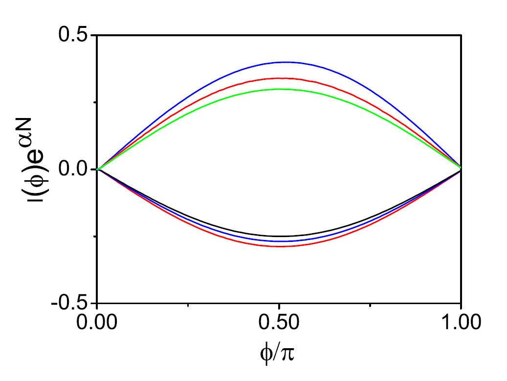
Figure 45: Josephson current-phase relation for the quantum dot array model analyzed in Ref. Bergeret et al. (2007) with $U=10\Delta$ at half-filling. The curves in the positive half plane correspond to $N=2,4$ and 6 (from top to bottom) while those taking negative values correspond to $N=1,3$ and 5 (from bottom to top). The current is scaled by and exponential factor $\exp{\alpha N}$ with $\alpha\simeq 1.8$ in units of $e\Delta/h$. Reprinted figure with permission from F.S. Bergeret et al., Physical Review B 76, 174510, 2007 Bergeret et al. (2007). Copyright (2007) by the American Physical Society.

VI.2 Multilevel quantum dots

So far only the single-level Anderson model has been considered for describing an individual quantum dot. A proper description of actual physical realizations of quantum dots could require to consider a multilevel generalization of this model. This has been already pointed out in connection with the experiments of Ref. van Dam et al. (2006) on InAs nanowires, whose results where qualitatively accounted for using a multilevel model in which two orbitals with different parity were involved.

Figure 46: Josephson current at $\phi=\pi/2$ in the multilevel S-QD-S model of Ref. Shimizu et al. (1998) as a function of the level position for the cases $n=1$ (a), $n=2$ (b) and $n=3$ (c), where $n$ denotes the level degeneracy. The dotted lines indicate the evolution of the dot total charge $n_{d}$. Reprinted figure with permission from Y. Shimizu et al., Journal of the Physical Society of Japan 67, 1525, 1998 Shimizu et al. (1998). Copyright (1998) by the Physical Society of Japan.

Multilevel effects in the Josephson current through a QD were first addressed in Ref. Shimizu et al. (1998) by means of the Hartree-Fock approximation. The authors showed that when non-diagonal processes involving different dot levels are relevant the system can behave as a $\pi$-junction even in the absence of a magnetic ground state. This is illustrated in Fig. 46 where the Josephson current at $\phi=\pi/2$ is plotted as a function of the dot levels position, $\epsilon_{0}$, for the cases with 1, 2 and 3 levels and including diagonal and non-diagonal couplings to the leads with the same value $\Gamma$. One can clearly notice that whereas in the lower panel (single level) the $\pi$-phase is only present for odd number of electrons ($n_{d}=1$) in the 2 and 3 level cases (panels b and c) the $\pi$ behavior is also present for even occupancy plateaus.

Similar ideas were discussed in Ref. Rozhkov et al. (2001) for a multilevel situation with nearly degenerate levels ($\delta\epsilon\ll\Delta$) connected at the same two points to the leads and using the cotunneling approach. The authors pointed out that the $\pi$-junction behavior is linked to two-particle processes in which one of the electrons proceeds through an occupied state and the other through an empty one.

Further analysis of this multilevel case was presented in Ref. Lee et al. (2010) using both perturbation theory (cotunneling approach) and NRG calculations. They considered a two-level situation coupled in parallel to single channel leads and including an exchange term $J$ between the electron spins in each dot level. In the normal case this exchange term for $J<0$ would drive a singlet-triplet transition. Two different situations are distinguished: a case in which the two orbitals have the same ”parity” (i.e. ${\mbox{s}ign}(t_{1L}*t_{1R})={\mbox{s}ign}(t_{2L}*t_{2R})$, where $t_{j\alpha}$ are the hopping from the $j$ level to the lead $\alpha$) and a case in which the parities are different. In the first case and for $t_{1L}/t_{1R}=t_{2L}/t_{2R}$ the dot levels are only coupled to the symmetric combination of the two leads, yielding an effective one channel problem. In the second case the problem is equivalent to a two channel two impurity model with exchange coupling.

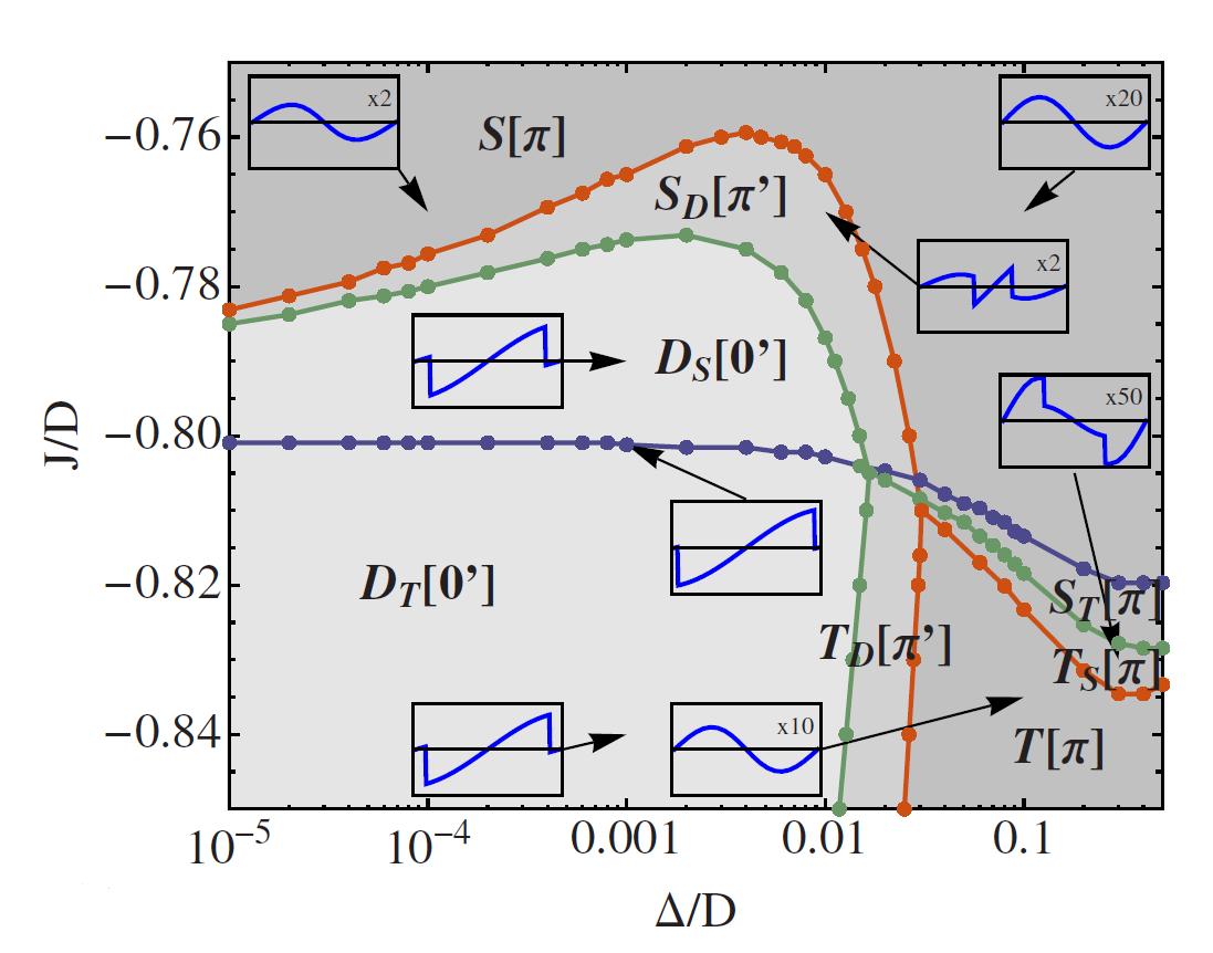
Figure 47: Phase diagram in the $J-\Delta$ plane for the two level dot model of Ref. Lee et al. (2010) corresponding to an effective one channel situation with symmetric coupling to the leads. The notation for the different phases is indicated in the main text. Reprinted figure with permission from M. Lee et al., Physical Review B 81, 155114, 2010 Lee et al. (2010). Copyright (2010) by the American Physical Society.

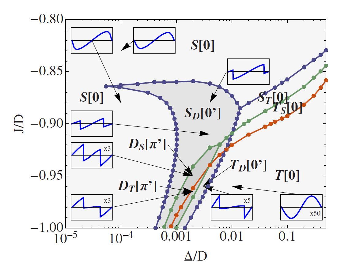
Figure 48: Same as Fig. 47 for the case corresponding to an effective two-channel two-impurity model. Reprinted figure with permission from M. Lee et al., Physical Review B 81, 155114, 2010 Lee et al. (2010). Copyright (2010) by the American Physical Society.

The system exhibits a very rich phase diagram depending on the several model parameters. For illustration we show in Fig. 47 and 48 the obtained phase diagrams in the $\Delta,J$ plane for the single channel and the two channel cases respectively for symmetric coupling to the leads. The different phases are denoted by a capital letter indicating the spin of the dominant ground state, which can be either $S$, $D$, or $T$ for spin 0, 1/2 or 1. In the case of mixed phases where the ground state changes with $\phi$ a subindex is included indicating the character of the metastable state. There is finally a label which can be either 0 or $\pi$ indicating the character of the current-phase relation in the dominant phase. The different types of current-phase relations are shown as insets in Figs. 47 and 48.

Figure 49: Phase diagram in the $U-\epsilon$ plane for the SU(4) Anderson model with superconducting leads analyzed in Ref. Zazunov et al. (2010) obtained in the ZBW approximation for $\Delta=10\Gamma$. White regions correspond to the $(S,T)=(0,0)$ and green to $(S,T)=(1/2,1/2)$. The black and blue regions correspond to mixed phases with $(S,T)=(0,0)$ at $\phi=0$ and $(S,T)=(1/2,1/2$ or $(S,T)=(1,0)-(0,1)$ at $\phi=\pi$ respectively. The right panel shows the evolution of the current-phase relation for $\epsilon/\Gamma=-5$ and several values of $U/\Gamma$. The small region in red inside the dashed white line corresponds to a $\pi^{\prime}$ mixed phase. Reprinted figure with permission from A. Zazunov et al., Physical Review B 81, 012502, 2010 Zazunov et al. (2010). Copyright (2010) by the American Physical Society.

Another multilevel situation which has been recently analyzed is the case of a four-fold degenerate level coupled to multichannel leads Zazunov et al. (2010). This situation has been found in experiments on high quality CNT quantum dots with normal leads showing clear signatures of four-fold degeneracy both in the Coulomb blockade and in the Kondo regimes Jarillo-Herrero et al. (2005, 2007). The SU(4) Kondo effect has been analyzed in the normal case by several authors like Yeyati et al. (1999), Choi et al. (2005b) and Lim et al. (2006). In Ref. Zazunov et al. (2010) Zazunov et al. have studied the Josephson effect in this case by considering a generalized SU(4) Anderson model with superconducting leads. They obtained analytical results in two opposite regimes corresponding to the deep Kondo limit $T_{K}\gg\Delta$ and the cotunneling limit. In the first case they obtained a current-phase relation which corresponds to the superposition of effective non-interacting channels with renormalized transmission $\tau=1/2$, therefore deviating from the SU(2) case where the unitary limit can be reached. In the cotunneling case with $U\rightarrow\infty$ a 0-$\pi$ transition at $\epsilon_{0}=0$ was obtained, as in the SU(2) case (see Ref. Glazman and Matveev (1989)) but with a different ratio of the critical currents $I_{c}(-|\epsilon_{0}|)/I_{c}(|\epsilon_{0}|)=-1/4$. The reduction of this ratio by a factor 2 with respect to the SU(2) case can be readily understood by considering the number of processes leading to Cooper pair transfer through the dot.

The authors also analyzed numerically the phase diagram of the model in the regime $\Delta\gg\Gamma$. A first insight is obtained by taking the limit $\Delta\rightarrow\infty$ in which case the relevant Hilbert space is reduced to the $2^{4}$ dot states. Conservation of the total spin, $S$, and orbital pseudo-spin, $T$, allows to further decouple this Hilbert space into three different sectors: $(S,T)=(0,0)$, $(S,T)=(1/2,1/2)$ and $(S,T)=(1,0)$ or $(0,1)$ (these last two are degenerate in the SU(4) case). The main features of the phase diagram obtained in this limit were shown to be preserved in the finite $\Delta\gg\Gamma$ regime, which was analyzed by means of the zero band-width model for the leads. The phase diagram, illustrated in Fig. 49, is essentially the same as in the $\Delta\rightarrow\infty$ limit except for two properties: first, the appearance of tiny $\pi^{\prime}$ type mixed phase (indicated by the red regions in Fig. 49) and second by the change in the character of the current-phase relation of the $(S,T)=(1/2,1/2)$ with increasing $U$. The panel on the right shows that this relation evolve with $U/\Delta$: while for $\Delta\gg U$ it is typically of 0 type, for $U>\Delta$ it becomes of $\pi$ type.

In closing this subsection we mention the recent appearance of a work by Lim et al. analyzing the effect of including spin-orbit interactions within this model Lim et al. (2011), which can be relevant for small radius CTNs Kuemmeth et al. (2008).

VI.3 Multidot-multiterminal systems with normal and superconducting leads

VI.3.1 Josephson effect through a quantum dot in a three terminal configuration

The Josephson effect through a single dot coupled to two superconductors and to a third normal lead has been analyzed by several authors. This configuration is schematically depicted in the upper panel of Fig. 50. An interesting non-equilibrium enhancement of the Josephson effect was predicted in Ref. Pala et al. (2007). The authors applied the real time diagrammatic approach commented in Subsect. III.3 with the tunneling rates to the leads calculated to the first order in $\Gamma_{S,N}$. They found that a significant Josephson current can be induced by the voltage bias applied to the normal leads even in the situation $\Gamma_{S}<k_{B}T$ where the equilibrium Josephson current would be negligible.

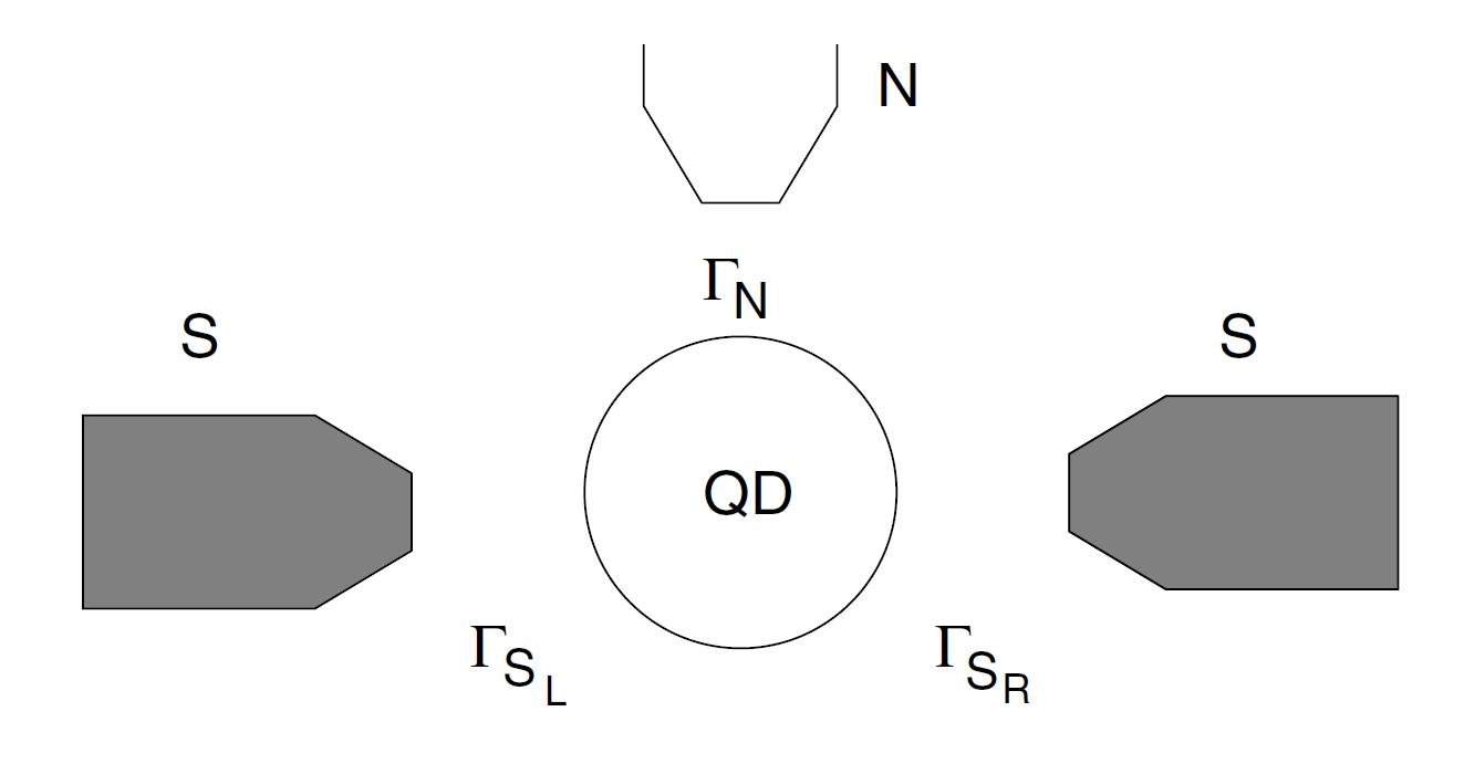
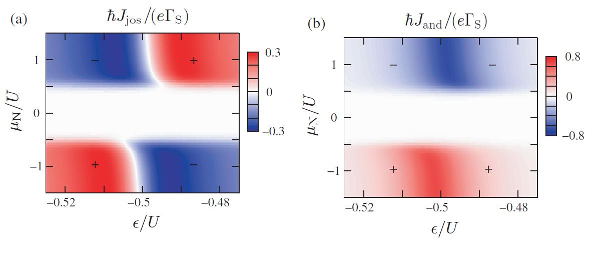
Figure 50: Color map of the Josephson critical current (lower left panel) and Andreev current (lower right panel) for the QD dot coupled to two superconducting leads and an additional voltage biased normal one in the $\mu_{N}/U-\epsilon/U$ plane. The upper panel gives a schematic representation of the setup considered in this work. Reprinted figure with permission from M. Pala et al., New Journal of Physics 9, 278, 2007 Pala et al. (2007). Copyright (2007) by IOP Publishing Ltd.

Fig. 50 shows a color map of the Josephson critical current as a function of both the level position and the chemical potential on the normal lead, $\mu_{N}$. One can notice the presence of a white region for $|\mu_{N}|\sim<U/2$ where the Josephson current is negligible. Outside this region it becomes of the order of $\sim e\Gamma_{S}/\hbar$ and exhibits a transition from 0 to $\pi$ behavior depending on the level position. The origin of this peculiar behavior can be traced to the enhancement of the proximity effect pairing amplitude on the dot due to the non-equilibrium population which increases the double population probability that is strongly suppressed at $\mu_{N}=0$ due to the charging energy. In a subsequent publication by the same group Governale et al. (2008) the authors considered the same effect in the limit $\Delta\rightarrow\infty$ which allows to account for the Josephson effect to all orders in $\Gamma_{S}$. The results obtained are qualitatively similar and allow to identify the lines separating different regions with the Andreev bound states of the S-QD-S system.

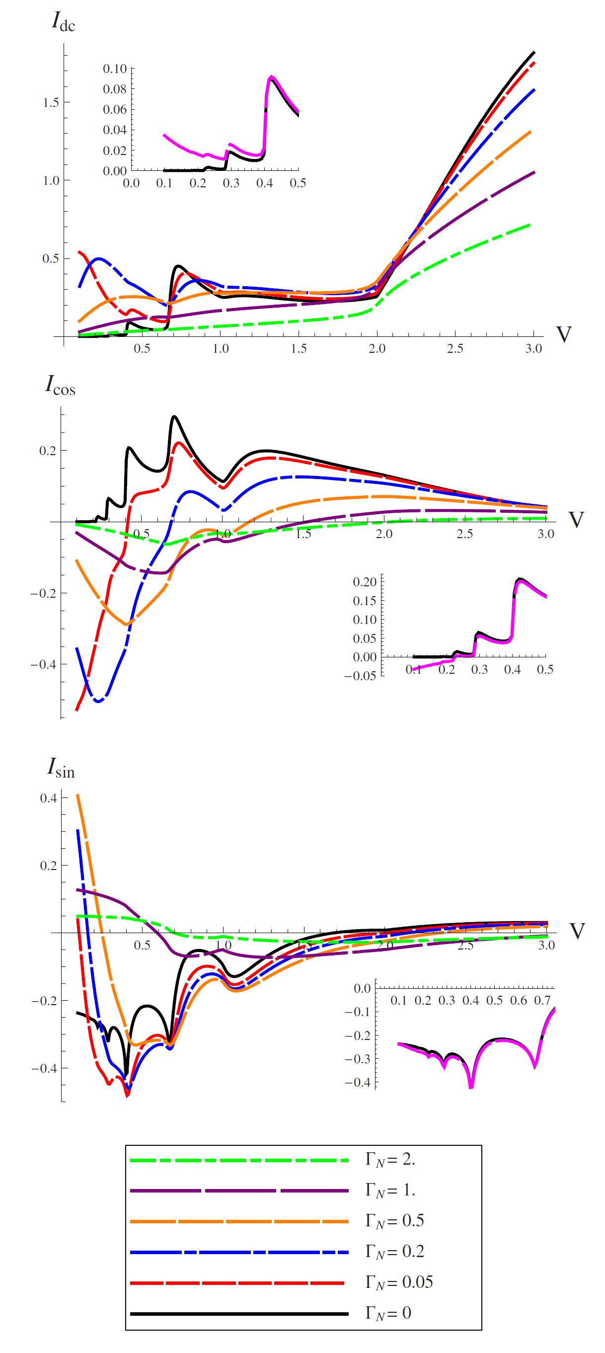
Figure 51: dc and the two first harmonics of the current-voltage characteristic of a non-interacting single level S-QD-S system with an additional normal lead connected to the dot with increasing coupling $\Gamma_{N}$ analyzed in Ref Jonckheere et al. (2009b). The other parameters are $\epsilon_{0}$ and $\Gamma_{S}=0.2\Delta$. The insets show the comparison of the dc current and the corresponding harmonics for $\Gamma_{N}=0$ (black line) and $\Gamma_{N}=0.02\Delta$ (red line). Reprinted figure with permission from T. Jonckheere et al., Physical Review B 80, 184510, 2009 Jonckheere et al. (2009b). Copyright (2009) by the American Physical Society.

It should be also mentioned within this context the work by Jonckheere et al. Jonckheere et al. (2009b) in which the effect of a third normal lead on the ac Josephson effect in a non-interacting voltage biased S-QD-S system was analyzed. The main idea of this work was to study the transition from the coherent MAR regime to the incoherent limit controlled by the coupling $\Gamma_{N}$ to the normal lead. They show that while the dc Josephson current exhibits a monotonous decrease with increasing $\Gamma_{N}$ the behavior of the dc quasiparticle current and its first ac harmonics have a much more involved evolution, which is illustrated in Fig. 51.

VI.3.2 Andreev transport through double quantum dots

Andreev transport in double quantum dot systems connected to normal and superconducting leads has been studied so far in a few works. Tanaka et al. Tanaka et al. (2008) considered the case of a T-shape geometry where a central dot is coupled to both electrodes and a second dot is only side-coupled to the central one, as shown in the upper panel of Fig. 52. The authors used the NRG method in the $\Delta\rightarrow\infty$ limit where, as discussed in Subsect. III.4, the superconducting lead acts as a simple boundary condition for Andreev reflection. They focused in the case where interactions are neglected in the central QD analyzing the effect of increasing $U$ in the lateral dot on the conductance through the system. The results of Fig. 52 show that the Andreev conductance gradually approaches the unitary limit as the side dot $U$ increases for the case $\Gamma_{N}=t$, where $t$ is the hopping between the two dots. On the other hand, for smaller values of $\Gamma_{N}$ the evolution of the conductance with $U$ is non-monotonous exhibiting for the symmetric case first an increase followed by a decrease. In this work it was also shown that the conductance in the electron-hole symmetric case can be tuned to the unitary limit for fixed $U$ by varying the coupling to the superconducting lead $\Gamma_{S}$. This possibility is analogous to the one already discussed for the single SQDN system in Sect. IV.

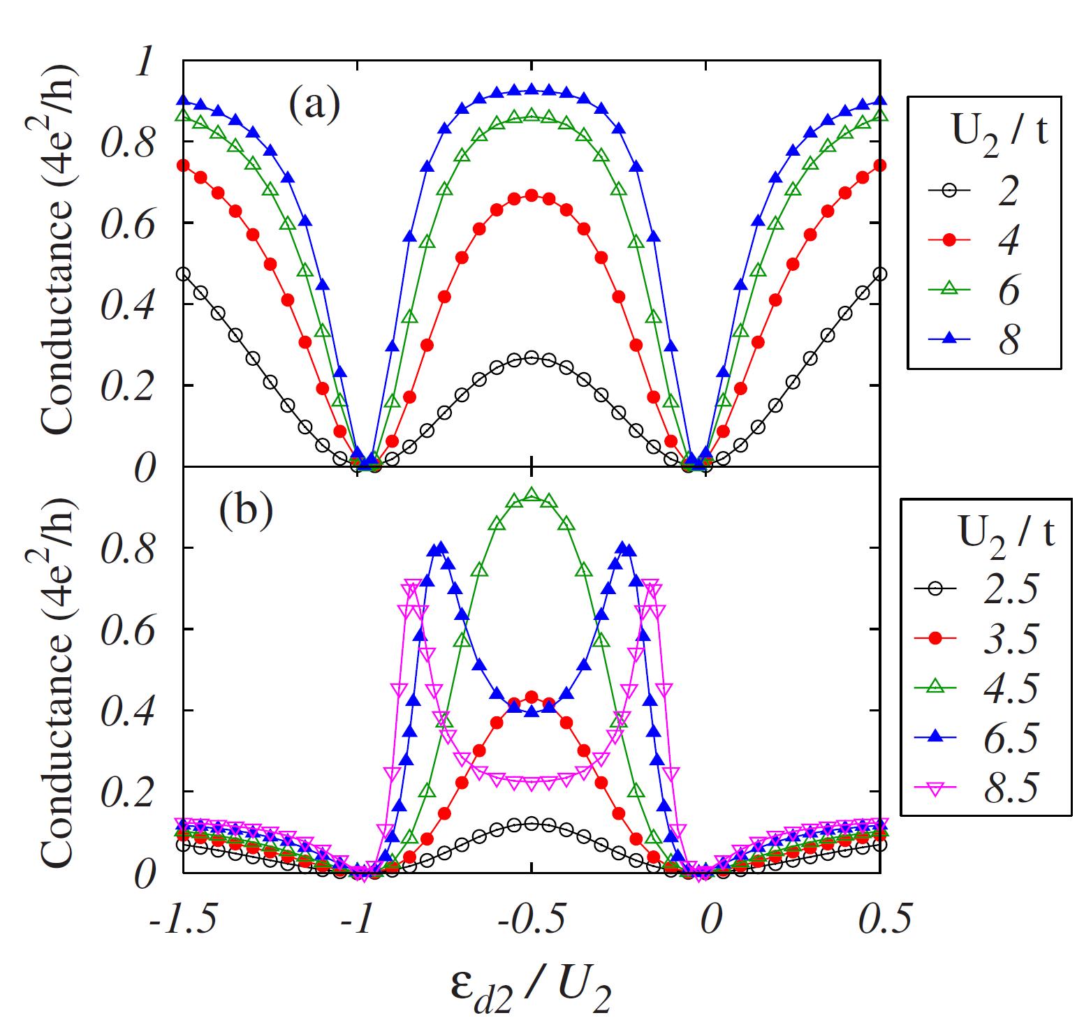
Figure 52: Linear conductance for the side coupled dot between a normal and a superconducting lead considered in Ref. Tanaka et al. (2008) as a function of the lateral dot level $\epsilon_{2}$ and for different values of the corresponding Coulomb interaction parameter $U_{2}$. The upper panel shows a schematic representation of the setup considered in this work. Reprinted figure with permission from Y. Tanaka et al., Physical Review B 78, 035444, 2008 Tanaka et al. (2008). Copyright (2008) by the American Physical Society.

In a subsequent paper Tanaka et al. (2010), the same authors considered the case of a double QD in series connected to a normal and a superconducting lead (see upper panel of Fig. 53) using the same theoretical approach. They first showed that for the case where the dot coupled to the normal lead is in the electron-hole symmetric condition the problem can be mapped into an effective normal two impurity Anderson model in terms of the Bogoliubov operators. Furthermore, this transformation allows to calculate the conductance using the Friedel sum rule in terms of a phase-shift given by

$$G=\frac{4e^{2}}{h}\left(\frac{\Gamma_{S}}{E}\right)\sin(\pi{\cal Q}),$$ (42)

where $E=\sqrt{\epsilon_{2}^{2}+\Gamma_{S}^{2}}$, $\epsilon_{2}$ being the level for the dot coupled to the superconductor and ${\cal Q}=\sum_{\sigma}\left(<\gamma^{\dagger}_{1\sigma}\gamma_{1\sigma}>+<\gamma^{\dagger}_{2\sigma}\gamma_{2\sigma}>\right)$, $\gamma_{i\sigma}$ indicating the Bogoliubov operators. The authors identified three different regimes. For small $t$ and $U<2\Gamma_{s}$ a regime corresponding to the a local superconducting singlet is found while for $U>2\Gamma_{s}$ the Kondo singlet state is formed. On the other hand, for large $t$ the antiferromagnetic coupling between the dots dominates. The behavior of the conductance in these three different regimes is summarized in Fig. 53. As can be observed, for sufficiently small $U/\Gamma_{s}$ the conductance can reach the unitary limit, the maximum displacing towards smaller $t$ values as $U$ increases and eventually for $U/\Gamma_{s}\sim>2$ the unitary limit cannot be reached. A surprising feature appears for $U/\Gamma_{s}\sim 2$ where the conductance reaches the unitary limit for two different $t$ values, indicated by the dashed rectangle in Fig. 53.

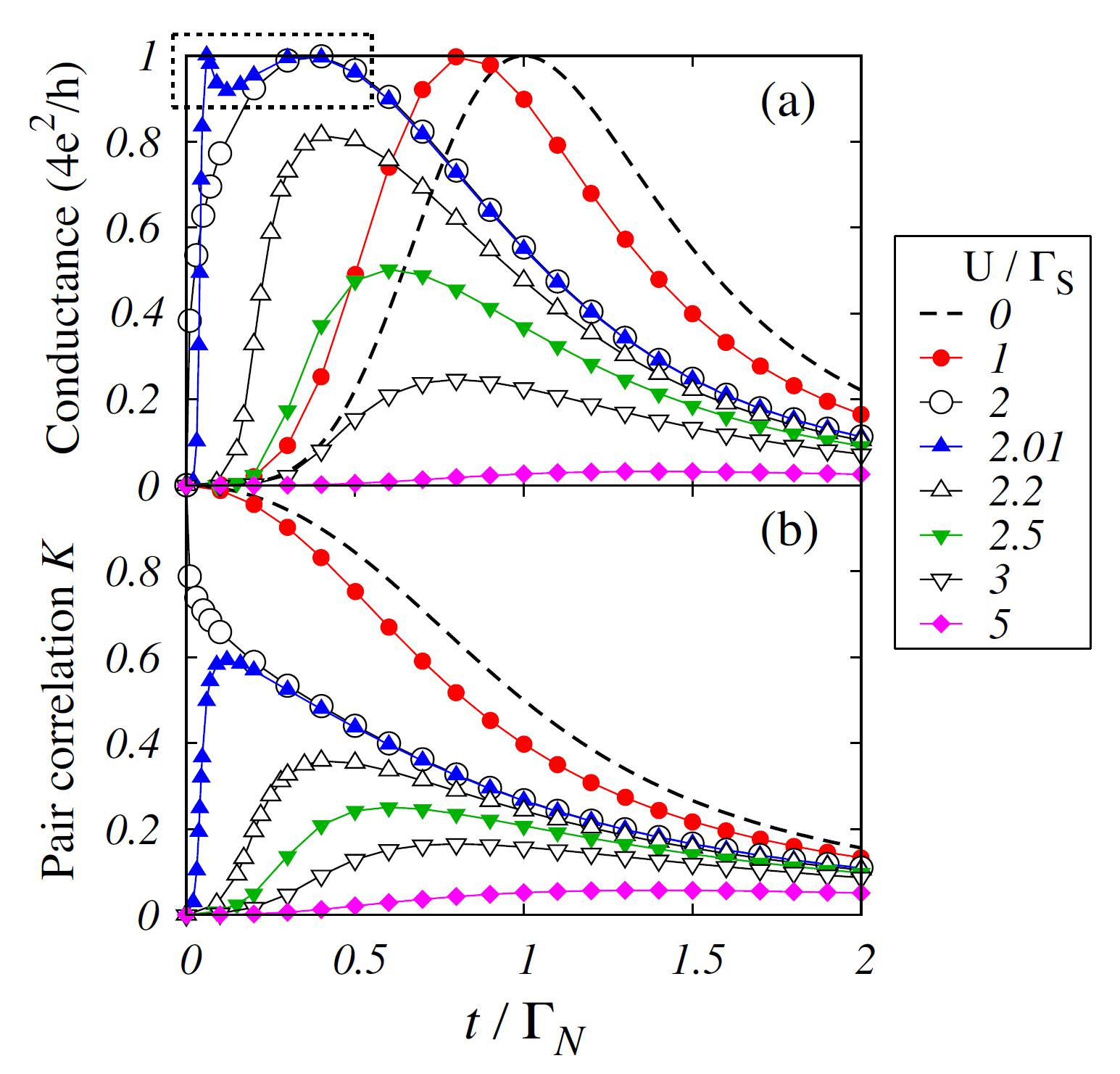
Figure 53: (a) Linear conductance for the series double quantum dot between a normal and a superconducting lead discussed in Ref. Tanaka et al. (2010) as a function of the interdot tunneling $t$ and for different values of $U/\Gamma_{s}$. Panel (b) shows the corresponding induced pairing correlation in the dots region. The results were obtained using the NRG method in the $\Delta\rightarrow\infty$ limit. Upper panel: setup considered in this work. Reprinted figure with permission from Y. Tanaka et al., Physical Review B 81, 075404, 2010 Tanaka et al. (2010). Copyright (2010) by the American Physical Society.

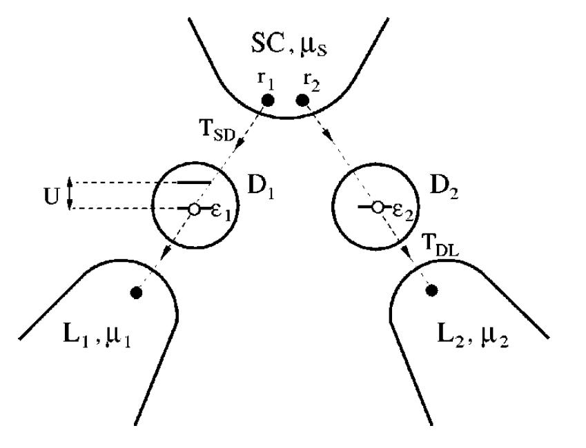
Figure 54: Schematic representation of a double quantum dot coupled to a central superconducting and two lateral normal leads in the proposal of Ref. Recher et al. (2001) for producing entangled electron pairs by means of non-local Andreev processes. Reprinted figure with permission from P. Recher et al., Physical Review B 63, 165314, 2001 Recher et al. (2001). Copyright (2001) by the American Physical Society.

VI.3.3 Non-local Andreev transport through single or double quantum dots

Double dots coupled to several normal and superconducting leads are receiving recently considerable attention in connection to the possibility of producing non-local entangled electrons from the splitting of Cooper pairs Recher et al. (2001); Hofstetter et al. (2009); Herrmann et al. (2010). The basic ideas were first put forward in Ref. Recher et al. (2001) where the multiterminal geometry of Fig. 54 was considered. In this configuration, when a Cooper pair is injected from the SC lead it can either be transmitted as a whole to one of the normal leads by a local Andreev process or split with each of the electrons in the pair transmitted to a different lead (corresponding to a non-local or crossed Andreev reflection process). The advantage of the DQD set up is twofold: on the one side it allows to tune independently the two dot levels and on the other hand Coulomb interactions could be used to favor the splitting processes compared to the local ones. While this issue is of a great current interest it goes beyond the scope of the present review. We would just mention several works addressing the non-local Andreev transport involving quantum dots and multiterminal configurations in Refs. Futterer et al. (2009); Eldridge et al. (2010).

VII Concluding remarks

In this review article we have summarized the most relevant published work related to superconducting transport in quantum dots systems. The large variety of topics that we have covered give an indication of the great activity which this field has shown in recent years. Due to the limited space it has become necessary to restrict somehow its content. For this purpose we have chosen to give priority to the more basic topics like Josephson effect and Andreev transport through single level quantum dots, and had left aside some interesting but more specialized situations like those involving ferromagnetic materials or unconventional superconductors. In the same way, we have not covered in this review the response of these systems to external ac fields, like photon assisted transport in S-QD-S Cho et al. (1999); Zhu et al. (2002) or N-QD-S systems Zhao (1998); Zhao and Wang (2001) and adiabatic pumping in NDQS systems Splettstoesser et al. (2007).

Even within the basic topics discussed in this review there remain several issues which are not completely understood and deserve further analysis. Among them we may point out: 1) the conflicting description of ABs within the different approximation schemes for S-QD-S systems, as discussed in Sect. III; 2) a more complete analysis of the phase diagrams of double QDs which so far has been restricted to certain parameter ranges, as commented in Sect. VI; 3) clarifying the interplay of Kondo and Andreev transport in N-QD-S beyond the linear regime (discussed in Sect. IV, and 4) extending the analysis of the MAR regime in S-QD-S beyond the limit of weak interactions analyzed in Sect. V.

It could be expected that the intense experimental and theoretical activity within this field will continue to grow in the next years. In addition to the already commented open issues there are several directions in which the research can be oriented. There are, on the one hand, other transport properties to be explored in the systems considered in this review, specially those related to current fluctuations. Some recent work address in fact the full-counting statistics in a non-interacting N-QD-S system Soller and Komnik (2011), but certainly there is a lot of open issues regarding the effect of interactions and the non-local current correlations in multiterminal configurations. In fact the analysis of these correlations can provide insight on the issue of non-local entanglement produced by the splitting of Cooper pairs, as has been shown in the case of diffusive samples Bignon et al. (2004) and ballistic conductors Samuelsson and Buttiker (2002).

On the other hand one could expect a renewed interest in these systems arising from the inclusion of recently discovered materials, like graphene and topological insulators. While graphene quantum dots have been already successfully produced experimentally and combined with superconductors like in Ref. Dirks et al. (2011), proposals of combining these systems with topological insulators are still on an speculative level Golub et al. (2011). We expect nevertheless that these issues would exhibit a great development in the near future.

References

- Affleck et al. (2000) Affleck, I., J.-S. Caux, and A. Zagoskin, 2000, Phys. Rev. B 62, 1433.
- Anderson (1961) Anderson, P., 1961, Phys. Rev. 124, 41.
- Andreev (1964) Andreev, A., 1964, Sov. Phys. JETP 19, 1228.
- Arnold (1987) Arnold, G., 1987, J. Low Temp. Phys. 68, 1.
- Averin and Bardas (1995) Averin, D., and A. Bardas, 1995, Phys. Rev. Lett. 75, 1831.
- Avishai et al. (2003) Avishai, Y., A. Golub, and A. D. Zaikin, 2003, Phys. Rev. B 67, 041301 (4pp).
- Bauer et al. (2007) Bauer, J., A. Oguri, and A. Hewson, 2007, J. Phys.: Cond. Matt. 19, 486211 (19pp).
- Beenakker (1992) Beenakker, C., 1992, Phys. Rev. B 46, 12841.
- Beenakker (1997) Beenakker, C., 1997, Rev. Mod. Phys. 69, 731.
- Benjamin et al. (2007) Benjamin, C., T. Jonckheere, A. Zazunov, and T. Martin, 2007, Eur. Phys. J. B 57, 279.
- Bergeret et al. (2006) Bergeret, F. S., A. L. Yeyati, and A. Martín-Rodero, 2006, Phys. Rev. B 74, 132505 (4pp).
- Bergeret et al. (2007) Bergeret, F. S., A. L. Yeyati, and A. Martín-Rodero, 2007, Phys. Rev. B 76, 174510 (6pp).
- Bickers (1987) Bickers, N., 1987, Rev. Mod. Phys. 59, 845.
- Bignon et al. (2004) Bignon, G., M. Houzet, F. Pistolesi, and F. Hekking, 2004, Europhys. Lett. 67, 110.
- Bratus et al. (1995) Bratus, E., V. Shumeiko, and G. Wendin, 1995, Phys. Rev. Lett. 74, 2110.
- Buitelaar et al. (2003) Buitelaar, M. R., W. Belzig, T. Nussbaumer, B. Babic, C. Bruder, and C. Schönenberger, 2003, Phys. Rev. Lett. 91(5), 057005 (4pp).
- Buitelaar et al. (2002) Buitelaar, M. R., T. Nussbaumer, and C. Schönenberger, 2002, Phys. Rev. Lett. 89(25), 256801 (4pp).
- Buizert et al. (2007) Buizert, C., A. Oiwa, K. Shibata, K. Hirakawa, and S. Tarucha, 2007, Phys. Rev. Lett. 99, 136806 (4pp).
- Cho et al. (1999) Cho, S. Y., K. Kang, C. M. Ryu, and C. K. Kim, 1999, Super. Latt. Mic. 26(6), 405.
- Choi et al. (2004) Choi, M., M. Lee, K. Kang, and W. Belzig, 2004, Phys. Rev. B 70, 020502 (4pp).
- Choi et al. (2005a) Choi, M., M. Lee, K. Kang, and W. Belzig, 2005a, Phys. Rev. Lett. 94, 229701 (1pp).
- Choi et al. (2000) Choi, M. S., C. Bruder, and D. Loss, 2000, Phys. Rev. B 62(20), 13569.
- Choi et al. (2005b) Choi, M. S., R. López, and R. Aguado, 2005b, Phys. Rev. Lett. 95, 067204 (4pp).
- Clerk and Ambegaokar (2000) Clerk, A., and V. Ambegaokar, 2000, Phys. Rev. B 61, 9109.
- Clerk et al. (2000) Clerk, A. A., V. Ambegaokar, and S. Hershfield, 2000, Phys. Rev. B 61(5), 3555.
- Cleuziou et al. (2006) Cleuziou, J.-P., W. Wernsdorfer, V. Bouchiat, T. Ondarcuhu, and M. Monthioux, 2006, Nature 1, 53.
- Coleman (1984) Coleman, P., 1984, Phys. Rev. B 29, 3035.
- Cronenwett et al. (1998) Cronenwett, S., T. Oosterkamp, and L. Kouwenhoven, 1998, Science 24, 540.
- Cuevas et al. (1996) Cuevas, J., A. Martín-Rodero, and A. L. Yeyati, 1996, Phys. Rev. B 54, 7366.
- Cuevas et al. (2001) Cuevas, J. C., A. L. Yeyati, and A. Martín-Rodero, 2001, Phys. Rev. B 63, 094515 (5pp).
- Deacon et al. (2010a) Deacon, R., Y. Tanaka, A. Oiwa, K. Yosida, K. Shibata, K. Hirakawa, and S. Tarucha, 2010a, Phys.Rev. B 81, 121308 (4pp).
- Deacon et al. (2010b) Deacon, R. S., Y. Tanaka, A. Oiwa, R. Sakano, K. Yoshida, K. Shibata, K. Hirakawa, and S. Tarucha, 2010b, Phys. Rev. Lett. 104, 076805 (4pp).
- Dell’Anna et al. (2008) Dell’Anna, L., A. Zazunov, and R. Egger, 2008, Phys. Rev. B 77, 104525 (6pp).
- Dirks et al. (2011) Dirks, T., T. Hughes, S. Lal, B. Uchoa, Y. Chen, C. Chialvo, P. Goldbart, and N. Mason, 2011, Nature Phys. 7, 386.
- Domanski and Donabidowicz (2008) Domanski, T., and A. Donabidowicz, 2008, Phys. Rev. B 78, 073105 (4pp).
- Eichler et al. (2009) Eichler, A., R. Deblock, M. Weiss, C. Karrasch, V. Meden, C. Schönenberger, and H. Bouchiat, 2009, Phys. Rev. B 79, 161407 (4pp).
- Eichler et al. (2007) Eichler, A., M. Weiss, S. Oberholzer, C. Schönenberger, A. L. Yeyati, J. C. Cuevas, and A. Martín-Rodero, 2007, Phys. Rev. Lett. 99, 126602 (4pp).
- Eldridge et al. (2010) Eldridge, J., M. Pala, M. Governale, and J. König, 2010, Phys. Rev. B 82, 184507 (5pp).
- Fazio and Raimondi (1998) Fazio, R., and R. Raimondi, 1998, Phys. Rev. Lett. 80(13), 2913.
- Fazio and Raimondi (1999) Fazio, R., and R. Raimondi, 1999, Phys. Rev. Lett. 82, 4950 (1pp).
- Ferrer et al. (1986) Ferrer, J., A. Martín-Rodero, and F. Flores, 1986, Phys. Rev. B 36, 6149.
- Franceschi et al. (2010) Franceschi, S. D., L. Kouwenhoven, C. Schönenberger, and W. Wernsdorfer, 2010, Nature Nano. 5, 703.
- Futterer et al. (2009) Futterer, D., M. Governale, M. Pala, and J. König, 2009, Phys. Rev. B 79, 054505 (5pp).
- Glazman and Matveev (1989) Glazman, L., and K. Matveev, 1989, JETP Lett. 49, 659.
- Glazman and Raikh (1988) Glazman, L., and M. Raikh, 1988, JETP Lett. 47, 452.
- Goldhaber-Gordon et al. (1998) Goldhaber-Gordon, D., H. Shtrikman, D. Mahalu, D. Abusch-Magder, U. Meirav, and M. Kastner, 1998, Nature 391, 156.
- Golub et al. (2011) Golub, A., I. Kuzmenko, and Y. Avishai, 2011, arXiv:1105.0289 .
- Golubov et al. (2004) Golubov, A., M. Kupriyanov, and E. Il ichev, 2004, Rev. Mod. Phys. 76, 411.
- Governale et al. (2008) Governale, M., M. Pala, and J. König, 2008, Phys. Rev. B 77, 134513 (14pp).
- Graber et al. (2004) Graber, M. R., T. Nussbaumer, W. Belzig, and C. Shonenberger, 2004, Nanotechnology 15(7), S479.
- Grove-Rasmussen et al. (2007) Grove-Rasmussen, K., H. I. Jorgensen, and P. Lindelof, 2007, New J. Phys. 1, 124 (10pp).
- Herrmann et al. (2010) Herrmann, L., F. Portier, P. Roche, A. L. Yeyati, T. Kontos, and C. Strunk, 2010, Phys. Rev. Lett. 104, 026801 (4pp).
- Hewson (1993) Hewson, A., 1993, The Kondo problem to heavy fermions, Cambridge Studies in Magnetism (Cambridge University Press, Cambridge, UK).
- Hofstetter et al. (2009) Hofstetter, L., S. Csonka, J. Nygard, and C. Schönenberger, 2009, Nature 461, 960.
- Hur et al. (2006) Hur, K. L., P. Recher, E. Dupont, and D. Loss, 2006, Phys. Rev. Lett. 96, 106803 (4pp).
- Jarillo-Herrero et al. (2005) Jarillo-Herrero, P., J. Kong, H. van der Zant, C. Dekker, L. Kouwenhoven, and S. D. Franceschi, 2005, Nature 434, 484.
- Jarillo-Herrero et al. (2007) Jarillo-Herrero, P., J. Kong, H. van der Zant, C. Dekker, L. Kouwenhoven, and S. D. Franceschi, 2007, Phys. Rev. Lett. 99, 066801 (4pp).
- Jarillo-Herrero et al. (2006) Jarillo-Herrero, P., J. van Dam, and L. P. Kouwenhoven, 2006, Nature 439(23), 953.
- Johansson et al. (1999) Johansson, G., E. Bratus, V. Shumeiko, and G. Wendin, 1999, Phys.Rev. B 60, 1382.
- Jonckheere et al. (2009a) Jonckheere, T., A. Zazunov, K. V. Bayandin, V. Shumeiko, and T. Martin, 2009a, Phys. Rev. B 80, 184510 (11pp).
- Jonckheere et al. (2009b) Jonckheere, T., A. Zazunov, K. V. Bayandin, V. Shumeiko, and T. Martin, 2009b, Phys. Rev. B 80, 184510 (11pp).
- Jorgensen et al. (2007) Jorgensen, H. I., T. Novotný, K. Grove-Rasmussen, K. Flensberg, and P. Lindelof, 2007, Nano Lett. 7, 2441.
- Kang (1998) Kang, K., 1998, Phys. Rev. B 57(19), 11891.
- Karrasch et al. (2008) Karrasch, C., A. Oguri, and V. Meden, 2008, Phys. Rev. B 77, 024517 (14pp).
- Kastner (1993) Kastner, M., 1993, Phys. Today 46, 24.
- Kasumov et al. (2005) Kasumov, A., K. Tsukagoshi, M. Kawamura, T. Kobayashi, Y. Aoyagi, K. Senba, T. Kodama, H. Nishikawa, I. Ikemoto, K. Kikuchi, V. Volkov, Y. Kasumov, et al., 2005, Phys. Rev. B 72, 033414 (4pp).
- Klapwijk et al. (1982) Klapwijk, T., G. Blonder, and M. Tinkham, 1982, Physica B 109 & 110, 1657.
- Koerting et al. (2010) Koerting, V., B. Andersen, K. Flensberg, and J. Paaske, 2010, Phys.Rev. B 82, 245108 (12pp).
- König et al. (1996) König, J., J. Schmid, H. Schoeller, and G. Schon, 1996, Phys. Rev. B 54, 16820.
- Kotliar and Ruckenstein (1986) Kotliar, G., and A. Ruckenstein, 1986, Phys. Rev. Lett. 57, 1362.
- Kouwenhoven and Glazman (2001) Kouwenhoven, L., and L. Glazman, 2001, Physics World 14, 33.
- Krawiec and Wysokinski (2004) Krawiec, M., and K. Wysokinski, 2004, Supercond. Sci. Technol. 17, 103.
- Krishna-murthy et al. (1980) Krishna-murthy, H., J. Wilkins, and K. Wilson, 1980, Phys. Rev. B 21, 1003.
- Kuemmeth et al. (2008) Kuemmeth, F., S. Ilani1, D. C. Ralph, and P. McEuen, 2008, Nature 452, 448.
- Lee et al. (2010) Lee, M., T. Jonckheere, and T. Martin, 2010, Phys. Rev. B 81, 155114 (20pp).
- Lee and Ng (1988) Lee, P., and T. Ng, 1988, Phys. Phys. Lett. 47, 1768.
- Lim et al. (2011) Lim, J., R. Lopez, M. Choi, and R. Aguado, 2011, arXiv:1104.0513 .
- Lim and Choi (2008) Lim, J. S., and M. S. Choi, 2008, J. Phys.: Condens. Matter 20(41), 415225 (6pp).
- Lim et al. (2006) Lim, J. S., M. S. Choi, R. López, and R. Aguado, 2006, Phys. Rev. B 74, 205119 (4pp).
- López et al. (2007) López, R., M. S. Choi, and R. Aguado, 2007, Phys. Rev. B 75, 045132 (6pp).
- Luitz and Assaad (2010) Luitz, D., and F. Assaad, 2010, Phys. Rev. B 81, 024509 (16pp).
- Martín-Rodero et al. (1999a) Martín-Rodero, A., A. L. Yeyati, and J. Cuevas, 1999a, Superlattices Micro. 25, 925.
- Martín-Rodero et al. (1999b) Martín-Rodero, A., A. L. Yeyati, and J. Cuevas, 1999b, Superlattices Microstruct. 25, 925.
- Matsumoto (2001) Matsumoto, D., 2001, J. Phys. Soc. Jpn. 70(2), 492.
- Ng (1993) Ng, T. K., 1993, Phys. Rev. Lett. 70, 3635.
- Nygard et al. (2000) Nygard, J., D. Cobden, and P. Lindelof, 2000, Nature 408, 342.
- Octavio et al. (1983) Octavio, M., M. Tinkham, G. Blonder, and T. Klapwijk, 1983, Phys. Rev. B 27, 6739.
- Oguri et al. (2004) Oguri, A., Y. Tanaka, and A. C. Hewson, 2004, J. Phys. Soc. Jpn. 73(9), 2494.
- Pala et al. (2007) Pala, M., M. Governale, and J. König, 2007, New J. Phys. 9, 278 (10pp).
- Pillet et al. (2010) Pillet, J.-D., C. Quay, P. Morfin, C. Bena, A. L. Yeyati, and P. Joyez, 2010, Nature Phys. 6, 965.
- Ralph et al. (1995) Ralph, D., C. Black, and M. Tinkham, 1995, Phys. Rev. Lett. 74, 3241.
- Ralph and Burhman (1994) Ralph, D., and R. Burhman, 1994, Phys. Phys. Lett. 69, 2118.
- Recher et al. (2001) Recher, P., E. Sukhorukov, and D. Loss, 2001, Phys. Rev. B 63, 165314 (11pp).
- Roch et al. (2009) Roch, N., S. Florens, T. Costi, W. Wernsdorfer, and F. Balestro, 2009, Phys. Rev. Lett. 103, 197202 (4pp).
- Rozhkov and Arovas (2000) Rozhkov, A., and D. Arovas, 2000, Phys. Rev. B 62, 6687.
- Rozhkov et al. (2001) Rozhkov, A., D. Arovas, and F. Guinea, 2001, Phys. Rev. B 64, 233301 (4pp).
- Rozhkov and Arovas (1999) Rozhkov, A. V., and D. Arovas, 1999, Phys. Rev. Lett. 82, 2788.
- Samuelsson and Buttiker (2002) Samuelsson, P., and M. Buttiker, 2002, Phys. Rev. Lett. 89, 046601 (4pp).
- Scheer et al. (1998a) Scheer, E., N. Agraït, J. Cuevas, A. L. Yeyati, B. Ludoph, A. Martín-Rodero, G. R. Bollinger, J. van Ruitenbeek, and C. Urbina, 1998a, Nature 394, 154.
- Scheer et al. (1998b) Scheer, E., P. Joyez, D. Esteve, C. Urbina, and M. H. Devoret, 1998b, Phys. Rev. Lett. 78, 3535.
- Schwab and Raimondi (1999) Schwab, P., and R. Raimondi, 1999, Phys. Rev. B 59(3), 1637.
- Schweitzer and Czycholl (1990) Schweitzer, H., and G. Czycholl, 1990, Solid State Commun. 74, 735.
- Sellier et al. (2005) Sellier, G., T. Kopp, J. Kroha, and Y. S. Barash, 2005, Phys. Rev. B 72, 174502 (12pp).
- Shiba (1973) Shiba, H., 1973, Prog. Theor. Phys. 50, 50.
- Shimizu et al. (1998) Shimizu, Y., H. Horii, Y. Takane, and Y. Isawa, 1998, J. Phys. Soc. Jpn. 67, 1525.
- Siano and Egger (2004) Siano, F., and R. Egger, 2004, Phys. Rev. Lett. 93(4), 047002 (4pp).
- Siano and Egger (2005a) Siano, F., and R. Egger, 2005a, Phys. Rev. Lett. 94, 039902 (1pp).
- Siano and Egger (2005b) Siano, F., and R. Egger, 2005b, Phys. Rev. Lett. 94, 229702 (1pp).
- Soller and Komnik (2011) Soller, H., and A. Komnik, 2011, Eur. Phys. J. D 63, 3.
- Spivak and Kivelson (1964) Spivak, B., and S. Kivelson, 1964, Phys. Rev. B 43, 3740.
- Splettstoesser et al. (2007) Splettstoesser, J., M. Governale, J. K nig, F. Taddei, and R. Fazio, 2007, Phys. Rev. B 75, 235302 (10pp).
- Sun et al. (2001) Sun, Q. F., H. Guo, and T. H. Lin, 2001, Phys. Rev. Lett. 87(17), 176601 (4pp).
- Sun et al. (2002) Sun, Q. F., H. Guo, and J. Wang, 2002, Phys. Rev. B 65, 075315 (11pp).
- T. Meng and Simon (2009) T. Meng, S. F., and P. Simon, 2009, Phys. Rev. B 79, 224521 (10pp).
- Tanaka et al. (2007a) Tanaka, Y., N. Kawakami, and A. Oguri, 2007a, J. Phys. Soc. Jpn. 76(7), 074701.
- Tanaka et al. (2008) Tanaka, Y., N. Kawakami, and A. Oguri, 2008, Phys. Rev. B 78, 035444 (6pp).
- Tanaka et al. (2010) Tanaka, Y., N. Kawakami, and A. Oguri, 2010, Phys. Rev. B 81, 075404 (11pp).
- Tanaka et al. (2007b) Tanaka, Y., A. Oguri, and A. C. Hewson, 2007b, New J. Phys. 9, 115.
- van Dam et al. (2006) van Dam, J., Y. Nazarov, E. Bakkers, S. D. Franceschi, and L. Kouwenhoven, 2006, Nature 442(10), 667.
- Varma and Yafet (1976) Varma, C., and Y. Yafet, 1976, Phys. Rev. B 13, 2950.
- Vecino et al. (2004) Vecino, E., M. R. Buitelaar, A. Martín-Rodero, C. Schönenberger, and A. L. Yeyati, 2004, SSC 131, 625.
- Vecino et al. (2003) Vecino, E., A. Martín-Rodero, and A. L. Yeyati, 2003, Phys. Rev. B 68, 035105 (9pp).
- Whan and Orlando (1996) Whan, C. B., and T. P. Orlando, 1996, Phys. Rev. B 54(8), 5255.
- Wiegmann and Tsvelick (1983) Wiegmann, P., and A. Tsvelick, 1983, J. Phys. C: Solid State Phys. 12, 2281.
- Wilson (1975) Wilson, K., 1975, Rev. Mod. Phys. 47, 773.
- Yamada and Yoshida (1975) Yamada, K., and K. Yoshida, 1975, Prog. Theor. Phys. 53, 1286.
- Yamada et al. (2010) Yamada, Y., Y. Tanaka, and N. Kawakami, 2010, J. Phys. Soc. Jpn. 79(4), 043705.
- Yamada et al. (2011) Yamada, Y., Y. Tanaka, and N. Kawakami, 2011, Phys. Rev. B 84, 075484 (18pp).
- Yeyati et al. (2005) Yeyati, A. L., J. Cuevas, and A. Martín-Rodero, 2005, Phys. Rev. Lett. 95, 056804 (4pp).
- Yeyati et al. (1997) Yeyati, A. L., J. C. Cuevas, A. López-Dávalos, and A. Martín-Rodero, 1997, Phys. Rev. B 55(10), 6137.
- Yeyati et al. (1999) Yeyati, A. L., F. Flores, and A. Martín-Rodero, 1999, Phys. Rev. Lett. 83, 600.
- Yeyati et al. (1993) Yeyati, A. L., A. Martín-Rodero, and F. Flores, 1993, Phys. Rev. Lett. 71, 2991.
- Yeyati et al. (2003) Yeyati, A. L., A. Martín-Rodero, and E. Vecino, 2003, Phys. Rev. Lett. 91(26), 266802 (4pp).
- Yoshioka and Ohashi (2000) Yoshioka, T., and Y. Ohashi, 2000, J. Phys. Soc. Jpn. 69(6), 1812.
- Zazunov et al. (2006) Zazunov, A., R. Egger, C. Mora, and T. Martin, 2006, Phys. Rev. B 73, 214501 (7pp).
- Zazunov et al. (2010) Zazunov, A., A. L. Yeyati, and R. Egger, 2010, Phys. Rev. B 81, 012502 (4pp).
- Zhao (1998) Zhao, H. K., 1998, Phys. Rev. B 58(20), 13660.
- Zhao and Wang (2001) Zhao, H. K., and J. Wang, 2001, Phys. Rev. B 64, 094505 (10pp).
- Zhu et al. (2002) Zhu, Y., Q. F. Sun, and T. H. Lin, 2002, Phys. Rev. B 66, 085306 (5pp).
- Zitko et al. (2010) Zitko, R., M. Lee, R. López, R. Aguado, and M.-S. Choi, 2010, Phys. Rev. Lett. 105, 116803 (4pp).