Cold bosons in the Landauer setup

Abstract

We consider one dimensional potential trap that connects two reservoirs containing cold Bose atoms. The thermal current and single-particle bosonic Green functions are calculated under non-equilibrium conditions. The bosonic statistics leads to Luttinger liquid state with non-linear spectrum of collective modes. This results in suppression of thermal current at low temperatures and affects the single-particle Green functions.

I Introduction

Systems of ultracold Bose gases have recently attracted a great deal of experimental Kinoshita ; Hofferbeth ; Amerongen ; Paredes and theoretical attention, see Refs. Zwerger, ; Giamarchi, for reviews. A high control over experimental conditions, including geometry, density, and interaction strength, as well as absence of uncontrolled disorder allow one to explore new aspects of many-body physics. Among experimental achievements, the coherence of non-equilibrium Bose condensate was studied based on the interference measurement Hofferberth_2008 , correlations of density fluctuations were measured in Ref.Esteve, , and the distribution of the bosons over momenta was explored in Ref. Amerongen, ; Paredes, ; Richard, .

Unlike the classic example of a bulk Bose fluid (⁴He), atomic gases are usually realized in optical traps or in atom chips where magnetic and electric fields confine the system to a geometry with strong asymmetry with respect to three-dimensional rotations. In many experimental situations, one deals with arrays of quasi-1D systemsHofferbeth ; Richard ; Davidson . These geometrical restrictions strongly influence the dynamics as they lower the effective dimensionality of the system. Indeed, in three dimensions a Bose system undergoes a famous Bose-Einstein condensation, its thermodynamic properties are well accounted by the mean free theory Pitaevskii_book , while its hydrodynamics is governed by the Gross-Pitaevskii equation. On the other hand, in two dimensions and especially in one dimension fluctuations of the order parameter destroy the long range order, necessitating a more microscopic treatment. In this work we focus on the impact these effects have on transport properties of one-dimensional bosonic systems.

As is well known, a clean one-dimensional (1D) system forms a strongly correlated ground state, so-called Luttinger liquid (LL). Though this description holds for both, fermionic and bosonic systems, the bosonic character begets new properties in Luttinger liquid state. To explore these features, we consider Landauer type setup shown in Fig.1, where bosons are trapped in the system that consists of two reservoirs connected by a one dimensional “wire”.

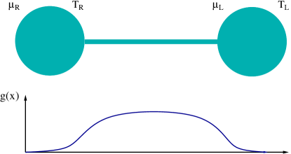
Figure 1: Two reservoirs with cold atoms are connected by one-dimensional trap. The temperatures and chemical potentials in the reservoirs are assumed to be different (upper panel); interaction strength $g(x)$ as a function of coordinate (lower panel).

Far-from-equilibrium realizations of Landauer setup have been recently studied in the framework of correlated 1D electronic (or, more generally, fermionic) systems. The tunneling spectroscopy of the non-equilibrium carbon nanotube have been measured in Ref. tunnel-spectroscopy, . The thermal current in the edge state of QHE was studied in Ref. tunnel-spectroscopy-qhe, . On the theory side, one can distinguish several types of non-equilibrium setups, ranging from partially gutman08 ; gutman09 to fully non-equilibrium situations GGM_long2010 . In the partial-equilibrium setup, electrons coming from different reservoirs have different values of chemical potential and temperature. In the case of full non-equilibrium, electrons in the reservoirs are characterized by an arbitrary single-particle density matrix. Remarkably, correlation functions of the interacting many-body problem can be calculated exactly even in the latter case, and can be cast in terms of Fredholm determinants.

In this paper, we address analogous questions in the context of bosonic system. Though at this moment we are not aware of any direct experimental realization of Landauer-type setup for bosons, the idea seems experimentally feasible. Indeed, the confinement of bosons to 1D optical wire has been accomplished in Ref.Esteve, . Since the case of partial equilibrium seems to be more natural from the point of view of experimental realization, we focus on it in the current work. We assume that the interaction between the atoms is of a hard core type. Inside the reservoirs it plays little role, and we approximate the atoms there as an ideal Bose gas. Inside the 1D “wire” connecting the reservoirs the hard core repulsion can not be neglected. We thus describe the system by LL with spatially varying interaction parameter $g(x)$, see Fig.1. One of the key features distinguishing this bosonic setup from its fermionic counterpart is the absence of Fermi surface. In other words, the excitation spectrum of particles in the non-interacting regions of the system is quadratic. Another interesting realization of excitations with quadratic spectrum are transverse spin waves in a ferromagnetic Bose gasZvonarev .

The non-linearity of the excitation spectrum is known to have a significant impact on the properties of the LL. In the fermionic case it leads to a number of interesting and important effects, see Refs. Glazman2009, ; Glazman2010, ; Glazman-RMP, for reviews. However, for most characteristics of low-temperature dynamics of correlated electronic systems such non-linearity can be discarded. This is done indeed in the case of the standard LL model. In the present situation, the spectrum for weak interaction is not linear even in the leading approximation. This should be accounted for in the corresponding theory and may be expected to profoundly affect the results of our analysis.

To deal with a non-linear dispersion of the spectrum in the bosonic case, we use the so-called harmonic approximation Haldane . Remarkably, this approach accurately describes the system in both the “quasi-condensate” (weakly interacting Bose gas) and the LL (sufficiently strong repulsive interaction) regimes. Within this framework, we study the thermal current and single-particle Green functions. The latter contain information about the density of states and the distribution function of bosons, as well as about information about phase-coherence correlations that are probed in interference experiments Hofferbeth .

II Bosonization of bosons

We begin with the Hamiltonian

$$H=H_{0}+H_{\rm int}\,,$$ (1)

that consists of the free part (we set $\hbar=1$),

$$H_{0}=-\frac{1}{2m}\int dx\hat{\Psi}^{\dagger}\partial_{x}^{2}\hat{\Psi}\,,$$ (2)

and the interaction,

$$H_{\rm int}=\int dxdx^{\prime}\hat{\rho}(x)V(x,x^{\prime})\hat{\rho}(x^{\prime})\,.$$ (3)

Here we define the density of the bosonic field $\rho(x)=\Psi^{\dagger}(x)\Psi(x)$; the bosonic field $\Psi$ satisfies canonical commutation relations,

$$[\hat{\Psi}(x),\hat{\Psi}^{\dagger}(x^{\prime})]=\delta(x-x^{\prime})\,.$$ (4)

To analyze the problem we use the hydrodynamic approach Haldane , similar to the bosonization for fermionic systems. The term “bosonization” in the present context is, perhaps, not optimal since the original system is bosonic to begin with. What actually happens is a transformation from the original bosonic fields $\Psi_{B}$, $\Psi_{B}^{\dagger}$ to new collective degrees of freedom described by bosonic fields $\phi,\theta$. The original field operator is expressed in term of the new fields as Popov ,Haldane_note

$$\hat{\Psi}_{B}(x)=\sqrt{\rho+\hat{\Pi}(x)}e^{i\hat{\theta}(x)}\,.$$ (5)

Here the field $\hat{\phi}(x)$ is related to the smeared density $\hat{\rho}(x)=\rho+\hat{\Pi}(x)$ (where $\rho$ is the average density) via $\hat{\Pi}(x)=-\partial_{x}\hat{\phi}(x)/\pi$. The collective bosonic fields ($\hat{\phi},\hat{\theta}$) satisfy the commutation relation

$$[\hat{\phi}(x),\hat{\theta}(x^{\prime})]=\frac{i\pi}{2}\rm{sgn}(x-x^{\prime})\,\,.$$ (6)

The substitution of Eq. (5) into the Hamiltonian (1) leads to a hydrodynamic description of 1D bosons Pitaevskii_book . This is a non-linear theory that can be considerably simplified by using the harmonic approximation. Expanding the Hamiltonian in the fields $\theta,\phi$, one keeps terms only up to the quadratic level, which yields

$$H_{0}=\frac{1}{2m}\int dx\bigg{[}\frac{1}{4\rho}(\partial_{x}\hat{\rho})^{2}+\rho(\partial_{x}\hat{\theta})^{2}\bigg{]}\,.$$ (7)

The harmonic approximation allows us to account for the non-linear (in the present case quadratic) spectrum of the low energy sound mode in the collective theory. Its validity is restricted to the low-energy (large-density) regime, $T\ll{\rm max}\{\Lambda,\rho g\}$. Here $\Lambda=\rho^{2}/m$ is the bosonic counterpart of Fermi energy, and $g$ is the interaction strength introduced below.

Clearly, the harmonic approximation is not an exact theory. By neglecting the interaction between low-energy modes (represented by terms of higher order in $\hat{\rho}$ and $\hat{\theta}$ in the Hamiltonian), one discards relaxation precesses that are important, in particular, for thermal equilibration, drag, and thermoelectric effect Glazman2010 ; Glazman-RMP ; Khodas2006 ; Khodas2007 ; Aristov ; Gangardt-Kamenev . We will assume that our “wire” is not too long, so that neglecting these processes is justified. In that situation the harmonic approximation is sufficient to describe thermal transport and tunneling spectroscopy in the system.

In terms of the collective bosonic fields $\theta$ and $\phi$ we obtain

$$H_{0}=\int dx\bigg{[}\frac{1}{8\pi^{2}m\rho(x)}\left(\partial_{x}^{2}\phi\right)^{2}+\frac{\rho(x)}{2m}\left(\partial_{x}\hat{\theta}\right)^{2}\bigg{]}\,,$$

$$H_{\rm int}=\int dx\frac{g(x)}{\pi^{2}}\left(\partial_{x}\hat{\phi}\right)^{2}\,.$$ (8)

Here we model the interaction with a short range potential,

$$V(x,x^{\prime})=g(x)\delta(x-x^{\prime})\,.$$ (9)

Let us note that Eq. (II) in fact corresponds to the microscopic model (9) in the limit of weak interaction only. In the local interaction model (9), the large-$g$ limit yields the Tonks-Girardeau gasGirardeau that can be mapped onto a free-fermion model (characterized by the LL parameter $K=1$). However, it makes sense to consider $g$ in Eq. (II) as a phenomenological parameter of underlying LL model, which allows us to go beyond the Tonks-Girardeau limit. On a microscopic level, this corresponds to the replacement of the delta-like repulsion (9) by a finite-range hard-core interaction.

Equation (II) is the Hamiltonian of a 1D LL for interacting bosonic system in the harmonic approximation Giamarchi . As one clearly observes, the Hamiltonian (II) contains a fourth-order spatial derivative [the term $(\partial_{x}^{2}\hat{\phi})^{2}$], at odds with the standard fermionic LL model that contains only a second spatial derivative [$(\partial_{x}\hat{\phi})^{2}$]. For large values of the interaction constant, $\rho g\gg\rho^{2}/2m$, the fourth-derivative term is relatively small, leaving us with the standard LL with the interaction parameter $K^{2}=\pi^{2}\rho/2mg$. When the interaction is weakened, $\rho g\ll\rho^{2}/2m$, the standard (linear-spectrum) LL description is valid for the lowest temperatures only, $T\ll\rho g$. The LL parameter becomes larger for weaker interaction and tends to infinity in the limit of free bosons but the region of applicability of the standard LL theory vanishes in this limit.

In the general case, one should use the full theory (rather than the standard LL theory). The corresponding spectrum of bosonic excitations $\omega(q)$ is non-linearChalker , interpolating between quadratic ($\omega=q^{2}/2m$ for non-interacting bosons) and linear ($\omega=uq$ for strongly interacting bosons; $u$ being the sound velocity). Finally, we mention that the Hamiltonian (II) depends on the mean bosonic density, $\rho(x)$. To find the profile of the bosonic density, one needs to go beyond the LL description and solve the non-linear hydrodynamic equations, see Appendix B.4.

To deal with the non-equilibrium conditions, we use the Keldysh formalism. The fields on the upper and lower branches are labeled by $+$ and $-$ respectively. It is convenient to perform a rotation in Keldysh space

$$\phi,\bar{\phi}=(\phi_{+}\pm\phi_{-})/\sqrt{2}\,,$$ (10)

$$\theta,\bar{\theta}=(\theta_{+}\pm\theta_{-})/\sqrt{2}\,.$$ (11)

where we will refer to $(\phi,\theta)$ as classical and to $(\bar{\phi},\bar{\theta})$ as quantum componentsKamenev . We then find that the system is described by the following action

$$S=\frac{1}{2}\Phi^{T}D^{-1}\Phi\,,$$ (12)

where we have defined the vector $\Phi=(\phi,\theta,\bar{\phi},\bar{\theta})$  . The inverse propagator has a standard structure in the Keldysh space

$${D^{-1}}=\begin{pmatrix}0&(D^{-1})^{r}\\ (D^{-1})^{a}&(D^{-1})^{K}\end{pmatrix},$$ (13)

where each component is a matrix in the $\theta,\phi$ space. The inverse retarded propagator is given by

$$(D^{-1})^{r}=\begin{pmatrix}\hat{K}^{-1}&-\frac{i\omega_{+}}{2\pi}\partial_{x}\\ -\frac{i\omega_{+}}{2\pi}\partial_{x}&-\frac{1}{2m}\partial_{x}\rho\partial_{x}\end{pmatrix},$$ (14)

with

$$\hat{K}^{-1}=\frac{\partial_{x}}{8\pi^{2}m}\bigg{[}\frac{2\rho_{x}}{\rho^{2}}\partial_{x}-\frac{\rho_{x}^{2}}{\rho^{3}}+\partial_{x}\frac{1}{\rho}\partial_{x}-8mg\bigg{]}\partial_{x}$$

and $\omega_{+}=\omega+i0$. The advance component is related to the retarded one by complex conjugation, $(D^{-1})^{a}(\omega)=\left[(D^{-1})^{r}(\omega)\right]^{*}$. The Keldysh component $(D^{-1})^{K}$ carries information about the distribution functions in two reservoirs: right-moving modes coming from the left reservoir have the temperature $T_{R}$, while the left-moving modes coming from the right reservoir are characterized by the temperature $T_{L}$.

To simplify the analysis from now on we consider the large density limit, approximating the mean bosonic density $\rho(x)$ by a constant. Variation of the action with respect to the classical components of the fields $\theta$ and $\phi$ yields the saddle point equations

$$\left(-\frac{1}{8\pi^{2}m\rho}\partial_{x}^{4}+\partial_{x}\frac{g(x)}{\pi^{2}}\partial_{x}\right)\bar{\phi}_{\omega}+\frac{i\omega}{2\pi}\partial_{x}\bar{\theta}_{\omega}=0\,,$$

$$\frac{i\omega}{2\pi}\partial_{x}\bar{\phi}_{\omega}+\frac{\rho_{0}}{2m}\partial_{x}^{2}\bar{\theta}_{\omega}=0\,.$$ (15)

These two equations can be conveniently combined into the wave equation

$$\bigg{[}\omega^{2}+\partial_{x}\left(\frac{2\rho g(x)}{m}-\frac{1}{4m^{2}}\partial_{x}^{2}\right)\partial_{x}\bigg{]}J(\omega,x)=0\,,$$ (16)

where we have introduced $J=\pi^{-1}\partial_{x}\bar{\theta}$. Equation (16) describes propagation of plasmons inside the wire with dispersion that varies in space (as a result of the variation of $g(x)$). Due to these variation, a plasmon may experience scattering but the total number of plasmons is conserved. To make this conservation explicit, we multiply Eq. (16) by $J^{*}$ from the left and subtract a complex-conjugated equation. This yields the plasmons conservation law

$$\partial_{t}Q+\partial_{x}{\cal J}=0\,$$ (17)

which has a form of the continuity equation that states that the charge

$$Q=J\partial_{t}J^{*}-J^{*}\partial_{t}J$$ (18)

is carried by the current

$${\cal J}=\frac{2\rho g}{m}\left(J^{*}J_{x}-JJ^{*}_{x}\right)$$ (19)

$$-\frac{1}{4m^{2}}\left(J^{*}J_{xxx}-J^{*}_{x}J_{xx}-JJ^{*}_{xxx}+J_{x}J^{*}_{xx}\right)\,.$$

In a region with a constant interaction strength $g$ Eq. (16) yields the Bogolubov’s excitation spectrum for the acoustic phonons,

$$\omega_{q}^{2}=\frac{2\rho g}{m}q^{2}+\frac{q^{4}}{4m^{2}}\,.$$ (20)

This dispersion relation has four solutions, resulting in oscillating and exponentially decaying (growing) waves (see Fig. 2),

$$J_{\omega}(x)=Ae^{iqx}+Be^{-iqx}+Ce^{px}+De^{-px}\,,$$ (21)

where

$$q=\sqrt{2}m\sqrt{-g+\sqrt{g^{2}+\omega^{2}/m^{2}}},$$ (22)

$$p=\sqrt{2}m\sqrt{g+\sqrt{g^{2}+\omega^{2}/m^{2}}}.$$ (23)

We consider now the situation when the interaction strength changes from one value to another in a boundary region, see Fig. 2. If we consider the solution not too close to the boundary, the exponentially decaying components can be neglected, and the propagating waves are related via a scattering matrix. To take into account the different velocities of propagation, we define $a=\sqrt{u}A$, $b=\sqrt{u}B$, where $u_{q}=\frac{\partial\omega_{q}}{\partial q}$ is a sound velocity in corresponding region. It is easy to verify that coefficients $a$ and $b$ in different regions (see Fig. 3) are related

$$\left(\!\!\begin{array}[]{l}a_{2}\\ \\ b_{1}\end{array}\right)=S\left(\!\!\begin{array}[]{l}a_{1}\\ \\ b_{2}\end{array}\right)\,$$ (30)

through a unitary scattering matrix,

$$S=\begin{pmatrix}t&r\\ r^{\prime}&t^{\prime}\end{pmatrix},$$ (31)

with $|t|=|t^{\prime}|$ and $|r|=|r^{\prime}|$.

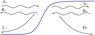
Figure 2: The boundary between the regions with different interaction constants. Propagating and decaying waves on both sides of the boundary are shown.

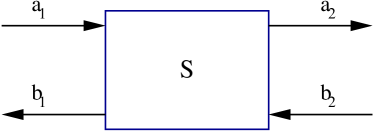
Figure 3: The scattering of plasmons at the boundary between regions with different values of interaction can be described by scattering matrix $S$.

The transmission coefficient has to be calculated for a particular realization $g(x)$ of the interaction in the boundary region. In the limiting case of an adiabatic barrier, when the interaction changes smoothly on the scale of the plasmon wave length, one finds the ideal transmission, $|t|=1$ and $r=0$. We focus on the opposite case of a sharp-step barrier, with interaction constant $g_{1}$ to the left of the boundary and $g_{2}$ to the right. To find the transmission and reflection amplitude of such a barrier, we derive matching conditions for the amplitudes at the boundary. For this purpose, we integrate Eq. (16) over a small region around the boundary. This leads to a requirement that $J$, $J^{\prime}$, $J^{\prime\prime}$, and $2\rho gJ^{\prime}-J^{\prime\prime\prime}/4m$ are continuous at the boundary [which implies that $J^{\prime\prime\prime}$ has a jump equal to $8m\rho J^{\prime}(g_{2}-g_{1})$]. These four conditions allow us to find the amplitudes $A_{2}$, $B_{1}$ of the outgoing waves and $C_{1}$, $D_{2}$ of the decaying waves for given amplitudes $A_{1}$ and $B_{2}$ of the incoming waves, and thus to establish the scattering matrix. We obtain the transmission

$$t=-\frac{2}{Z}\sqrt{q_{1}q_{2}\frac{(q_{1}+ip_{1})(q_{2}+ip_{2})}{(q_{1}-ip_{1})(q_{2}-ip_{2})}}$$ (32)

$$\times[8\pi m\rho p_{2}(g_{1}-g_{2})-(p_{1}+p_{2})(q_{1}^{2}+p_{2}^{2})]\,,$$

and the reflection amplitude

$$r=\frac{1}{Z}\frac{q_{2}+ip_{2}}{q_{2}-ip_{2}}\bigg{[}-(p_{1}+p_{2})(q_{1}+ip_{2})(q_{2}-ip_{1})(q_{1}-q_{2})$$

$$+8\pi m\rho(p_{1}q_{1}+p_{2}q_{2})(g_{2}-g_{1})\bigg{]}\,,$$ (33)

where we have introduced the notation

$$Z=(p_{1}+p_{2})(q_{1}+ip_{2})(q_{2}+ip_{1})(q_{1}+q_{2})$$

$$+8\pi m\rho(p_{1}q_{1}-p_{2}q_{2})(g_{2}-g_{1}).$$ (34)

For our model with non-interacting reservoirs, we now consider the case of the scattering between interacting and non interacting regions, i.e. $g_{1}=0$ and $g_{2}=g$. In this case the transmission amplitude is a function of a dimensionless parameter $s=\omega/2\pi\rho g$ with the asymptotics

$$t\left(s\right)=\left\{\begin{array}[]{l}-2^{3/4}s^{1/4},\,\,\,\,\,\text{for}\,\,s\ll 1\\ \\ 1,\,\,\,\,\,\,\,\,\text{for}\hskip 14.22636pts\gg 1.\\ \end{array}\right.$$ (35)

III Kinetics of 1D Bose fluid: Thermal current

In the preceding section, we have found the plasmon transmission coefficients at the boundaries between the interacting region and the reservoirs. Supplementing these results with the boundary conditions on the distribution functions of plasmons in the reservoirs, we straightforwardly calculate the distribution functions of the right and the left moving modes ($B_{R/L}$) inside the wire, see Fig. 4.

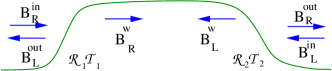
Figure 4: Distribution functions for transmitted and reflected plasmons inside the wire

For a wire longer than the thermal wave length of plasmons, the Fabry-Perot-type plasmon interference can be neglected, and one finds

$$B_{R}^{w}=\frac{{\cal T}_{1}}{1-{\cal R}_{1}{\cal R}_{2}}B_{R}^{(0)}+\frac{{\cal T}_{2}{\cal R}_{1}}{1-{\cal R}_{1}{\cal R}_{2}}B_{L}^{(0)}\,,$$

$$B_{L}^{w}=\frac{{\cal T}_{2}}{1-{\cal R}_{2}{\cal R}_{1}}B_{L}^{(0)}+\frac{{\cal T}_{1}{\cal R}_{2}}{1-{\cal R}_{2}{\cal R}_{1}}B_{R}^{(0)}\,,$$ (36)

where $B_{R}^{(0)}=\coth(\omega/2T_{R})$, $B_{L}^{(0)}=\coth(\omega/2T_{L})$, $T_{L}$ and $T_{R}$ are temperatures of the left and the right moving collective modes, ${\cal T}_{1}=|t_{1}|^{2}$, ${\cal T}_{2}=|t_{2}|^{2}$ are the transmission coefficients of the left and right barriers, and ${\cal R}_{j}=1-{\cal T}_{j}$ are the corresponding reflection coefficients. .

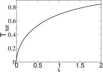
Figure 5: Total plasmon transmission for a system of two identical sharp barriers as a function of $s=\omega/2\pi\rho g$.

Using the plasmon distribution function one can calculate, in particular, the thermal current

$$I_{E}=\frac{1}{4\pi}\int_{0}^{\infty}d\omega\omega[B_{L}^{w}(\omega)-B_{R}^{w}(\omega)]\,.$$ (37)

Substituting Eq.(III) into Eq.(37), we find

$$I_{E}=\frac{1}{4\pi}\int_{0}^{\infty}d\omega\omega[B_{L}^{0}(\omega)-B_{R}^{0}(\omega)]{\cal T}_{\rm tot}(\omega)\,.$$ (38)

Here ${\cal T}_{\rm tot}$ is the total transmission coefficient

$${\cal T}_{\rm tot}(\omega)=\frac{{\cal T}_{1}(\omega){\cal T}_{2}(\omega)}{1-{\cal R}_{1}(\omega){\cal R}_{2}(\omega)}\,;$$ (39)

it is shown in Fig. 5 for the case of two sharp barriers characterized by the transmission amplitude (32).

Substituting ${\cal T}_{\rm tot}$ for the case of two sharp barriers into Eq. (38) and performing the frequency integration, we find

$$I_{E}={\cal F}_{E}(T_{L})-{\cal F}_{E}(T_{R})\,,$$ (40)

where

$${\cal F}_{E}(T)=\left\{\begin{array}[]{l}\frac{3}{8\pi}\frac{1}{\sqrt{\rho g}}\xi\left(\frac{5}{2}\right)T^{5/2},\,\,\,\,\,\text{for}\,\,T\ll 2\pi\rho g\\ \\ \frac{\pi}{12}T^{2}\,\,\,\,\,\,\,\,,\text{for}\,\,T\gg 2\pi\rho g\\ \end{array}\right.$$ (41)

In the limit of small temperature difference $\Delta T=T_{L}-T_{R}$ we have

$$I_{E}=\frac{\Delta T}{8\pi T^{2}}\int_{0}^{\infty}d\omega\frac{\omega^{2}}{\sinh^{2}\omega/2T}{\cal T}_{\rm tot}(\omega)\,,$$ (42)

where $T=\frac{T_{L}+T_{R}}{2}$. Eq.(42) can be cast in the scaling form

$$I_{E}=\Delta TTf\left(\frac{T}{2\pi\rho g}\right)\,.$$ (43)

The function $f$ entering Eq. (43) can be calculated numerically and is plotted in Fig. 6. It has the following asymptotic limits:

$$f\left(s\right)=\left\{\begin{array}[]{l}as^{1/2},\,\,\,\,\,\text{for}\,\,s\ll 1\,,\\ \\ \frac{\pi}{6},\,\,\,\,\,\,\,\,\text{for}\hskip 14.22636pts\gg 1\,,\\ \end{array}\right.$$ (44)

where $a\simeq 1.003$.

At relatively high temperatures, $T\gg\rho g$, we reproduce the thermal current of non-interacting bosonsRego , see Appendix A). This result can be considered as a thermal-current counterpart of the Landauer quantization of charge conductance: the numerical coefficient in the second line of Eqs. (41) and (44) is fully universal in 1D geometry and does not depend on the form of the spectrum, interaction strength, carrier statistics (fermions vs. bosons), etc. The only condition is the absence of back-scattering of plasmons. In the low-temperature regime, we find that the thermal current is suppressed due to reflection of the bosons on the boundary between interacting and non-interacting regions. This $T^{1/2}$ suppression of the thermal conductance distinguishes the bosonic setup from its fermionic counterpart.

Figure 6: Scaling function $f(s)$ governing the dependence of the heat current on $s=T/2\pi\rho g$, see Eq. (43)

IV Phase coherent dynamics: Green functions

We now proceed with the analysis of the single-particle Green functions of the original bosons,

$$G_{B}^{>}(x,\tau)=-i\langle\hat{\Psi}_{B}(x,t)\hat{\Psi}^{\dagger}_{B}(0,0)\rangle\,\,\,,$$

$$G_{B}^{<}(x,\tau)=-i\langle\hat{\Psi}^{\dagger}_{B}(0,0)\hat{\Psi}_{B}(x,t)\rangle\,\,\,,$$ (45)

that carry information about spectral properties (density of states and distribution functions) of the system. The results for the non-interacting case are well known; for completeness we present them in Appendix A. Our approach allows us to analyze the Green functions in a broad range of parameters, with the only assumption being $T\ll{\rm max}(\rho g,\rho^{2}/2m)$. To relate it to well-accepted terminology in the field Gangardt_2003 ; Gangardt_2009 , the harmonic approximation allows us to describe the system in the “Decoherent Quantum”, “Quasi-Condensate”, and “Tonks-Girardeau” regimes, and in the strong-interaction LL regime, $\rho g\gg T,\rho^{2}/2m$ (which is not realized in the delta-interaction model considered in Ref. Gangardt_2003, ; Gangardt_2009, ), as well as in crossovers between them.

Using the representation of the boson creation and annihilation operators in terms of the collective field, Eq. (5), we write the Green function as a correlation function of the harmonic fluid,

$$G^{\gtrless}(x,\tau)=-i\langle T_{K}\hat{\rho}_{\mp}^{1/2}(x,\tau)e^{i\hat{\theta}_{\mp}(x,\tau)}\hat{\rho}_{\pm}^{1/2}(0,0)e^{-i\hat{\theta}_{\pm}(0,0)}\rangle\,.$$ (46)

It is convenient to represent this correlation function as

$$G^{\gtrless}(X,\tau)=-i\rho\left(1-i\left(\frac{\partial}{\partial\alpha_{1}}+\frac{\partial}{\partial\alpha_{2}}\right)-\frac{\partial^{2}}{\partial\alpha_{1}\partial\alpha_{2}}\right)$$

$$\times\langle e^{i\int(d\omega)dxJ^{\gtrless}_{-\omega,x}\Phi^{T}(\omega,x)}\rangle\,.$$ (47)

Here we have defined a four-component “source” vector

$$J^{\gtrless}_{1,-\omega,x}=\frac{-1}{2\pi\rho\sqrt{2}}\frac{\partial}{\partial x}\bigg{[}e^{-i\omega\tau}\alpha_{1}\delta(x-X)+\alpha_{2}\delta(x)\bigg{]},$$

$$J^{\gtrless}_{2,-\omega,x}=\frac{1}{\sqrt{2}}\bigg{[}e^{-i\omega\tau}\delta(x-X)-\delta(x)\bigg{]}\,,$$

$$J^{\gtrless}_{3,-\omega,x}=\frac{\pm 1}{2\pi\rho\sqrt{2}}\frac{\partial}{\partial x}\bigg{[}e^{-i\omega\tau}\alpha_{1}\delta(x-X)-\alpha_{2}\delta(x)\bigg{]},$$

$$J^{\gtrless}_{4,-\omega,x}=\mp\frac{1}{\sqrt{2}}\bigg{[}e^{-i\omega\tau}\delta(x-X)+\delta(x)\bigg{]}\,,$$ (48)

and it is understood that one should set the sources $\alpha_{1,2}=0$ after the derivatives in Eq. (47) have been evaluated.

Since the action (12) is Gaussian, the functional integration over fields $\theta$ and $\phi$ can be easily performed, yielding

$$G^{\gtrless}(X,\tau)=-i\rho\left(1-i\left(\frac{\partial}{\partial\alpha_{1}}+\frac{\partial}{\partial\alpha_{2}}\right)-\frac{\partial^{2}}{\partial\alpha_{1}\partial\alpha_{2}}\right)$$

$$\exp\left(-\frac{i}{4}\int(d\omega)dx_{1}dx_{2}J^{\gtrless}_{-\omega,x_{1}}D_{\omega,x_{1},x_{2}}J^{\gtrless T}_{\omega,x_{2}}\right)\,.$$

Thus, the problem of calculation of the Green functions has been reduced to the calculation of the bosonic propagator

$$D=\begin{pmatrix}D^{K}&D^{r}\\ D^{a}&0\end{pmatrix}.$$ (49)

We now focus on the case of coinciding spatial points ($X=X^{\prime}$) deeply inside the interacting part of the wire (for $X\neq X^{\prime}$ see Appendix B.3). Expanding the bosonic density operator up to second order in $\phi$, and calculating Gaussian functional integral over the bosonic fields (see Appendix B.3 for technical details), we obtain

$$G^{\gtrless}(\tau)=-i\rho\bigg{(}1-\Phi_{1}^{\gtrless}(\tau)\bigg{)}e^{-\Phi_{2}^{\gtrless}(\tau)}\,.$$ (50)

Here we have defined the pre-exponential factor

$$\Phi^{\gtrless}_{1}(\tau)=\frac{m}{2\pi\rho}\int_{0}^{\infty}\frac{d\omega}{4\rho gq+q^{3}/m}\bigg{[}(B_{R}^{w}+B_{L}^{w})$$ (51)

$$\times\left(i\omega\sin\omega\tau-\frac{q^{2}}{4m}\cos\omega\tau\right)\pm\frac{iq^{2}}{2m}\sin\omega\tau\mp 2\omega\cos\omega\tau\bigg{)}\,,$$

and the exponential factor

$$\Phi^{\gtrless}_{2}(\tau)=\frac{m}{2\rho}\int_{0}^{\infty}\frac{d\omega}{2\pi}e^{-\omega/\Lambda}\frac{g+q^{2}/8m\rho}{q(g+q^{2}/4m\rho)}$$

$$\times\bigg{(}(B_{R}^{w}+B_{L}^{w})(1-\cos\omega\tau)\pm 2i\sin\omega\tau\bigg{)}\,.$$ (52)

In these formulas $q$ should be understood as related to $\omega$ via the dispersion law (22).

It is instructive to compare our results for the Green functions of a bosonic system in a partial non-equilibrium state, with their fermionic counterparts gutman09 . It is seen that the bosonic results differ in two respects: (i) the appearance of a pre-exponential factor and (ii) a more complicated form of the exponential factor reflecting the non-linear character of the spectrum of collective excitations.

In fact, Eq. (50) interpolates between the standard-LL results (applicable in the limit of strongly interacting bosons) and Eq.(62) which is valid for free bosons. The characteristic energy scale for the crossover between these two regimes is set by the interaction ($\omega_{0}=\rho g$). For energies well below $\omega_{0}$, the model behaves as a standard LL system (with a linear plasmonic spectrum). In this case the pre-exponential factor $\Phi_{1}$ is small (of the order of $T/\omega_{0}\ll 1$), and therefore can be neglected. The exponential factor $\Phi_{2}$ in this limit turns into the LL result of Ref. gutman09, (which, of course, reduces to the conventional LL formula in the equilibrium case). In the high-energy limit $({\rm max}\{\tau^{-1},T\}\gg\omega_{0})$ the spectrum of excitations is quadratic, and one recovers the free-boson results, see Appendix A.

V Summary

In this work, we have studied a system of bosonic atoms in a Landauer setup, subject to temperature and chemical potential difference. We have developed a non-equilibrium bosonization approach that describes the system within the harmonic approximation. This approach ignores the interaction between different collective modes but takes into account the non-linear dispersion of their spectrum.

We have studied the plasmon propagation in a two-terminal setup formed by two non-interacting reservoirs connected by an interacting 1D “wire”. The plasmon back-scattering is controlled by the dimensionless parameter $s\sim\omega/\rho g$, where $\omega$ is the plasmon frequency (whose characteristic value is set by the respective temperatures of the reservoirs), $\rho$ is the density of bosons, and $g$ the interaction strength. At large $s$, back-scattering is suppressed, and the thermal current acquires a universal value (that depends neither on the spectrum of the original particles nor on their statistics). In the low-temperature regime, reflection of plasmons is strong, and the thermal current exhibits a $T^{1/2}$ suppression compared to the universal value. As another application of this formalism, we have calculated the bosonic single particle Green function in the same non-equilibrium setup. The result interpolates between the conventional (linear spectrum) Luttinger-liquid and free-boson limits.

The approach developed in this work can be used to study other properties of the system, e.g., higher correlation functions or non-steady-state characteristics. A more ambitious perspective will be development of a general non-equilibrium bosonized theory of non-linear LL (formed by interacting fermionic or bosonic particles) including both non-linear spectral dispersion of plasmon modes and their coupling.

VI Acknowledgments

We thank N. Davidson, L. Khaykovich, and J. Schmiedmayer for useful discussions. Financial support by German-Israeli Foundation,the Israel Science Foundation, and the Minerva Center is gratefully acknowledged.

Appendix A Transport properties of free bosons

In this Appendix we summarize basic properties of non-interacting bosons, using the original description.

A.1 Landauer approach: Particle current

For the case of non-interacting bosons the particle current can be straightforwardly found within the Landauer approach:

$$I=\int_{0}^{\infty}d\epsilon\nu(\epsilon)v(\epsilon)[N_{L}(\epsilon)-N_{R}(\epsilon)]\,,$$ (53)

where $\nu$ is the density of states, $v$ the velocity, and $N_{j}$ the distribution function in the corresponding reservoir. Using the relation $\nu(\epsilon)v(\epsilon)=1/2\pi$, one finds the relation

$$I=\int_{0}^{\infty}\frac{d\epsilon}{2\pi}[N_{L}(\epsilon)-N_{R}(\epsilon)]\,.$$ (54)

Assuming Bose distributions with the same temperature $T$ and two different chemical potentials $\mu_{L}$, $\mu_{R}$ and performing the integration, we obtain

$$I=-\frac{T}{2\pi}\ln\left(\frac{1-e^{\mu_{L}/T}}{1-e^{\mu_{R}/T}}\right).$$ (55)

We note that the particle current is determined by the occupation numbers in both reservoirs at the bottom of the band (at $\epsilon=0$). In the linear response regime, expanding the current in the difference of chemical potentials, we find

$$I=\frac{1}{2\pi}(\mu_{L}-\mu_{R})N_{B}(\epsilon=0)\,.$$ (56)

To relate the occupation number at the bottom of the band to macroscopic parameters of the problem we compute the particle density

$$\int_{0}^{\infty}d\epsilon\nu(\epsilon)N_{B}(\epsilon)=\rho\,.$$ (57)

For $|\mu|\ll T$ one finds

$$\rho=T\sqrt{\frac{m}{|\mu|}}\,,$$ (58)

thus leading to $N_{B}(\epsilon=0)=\rho^{2}/mT$ and

$$I=\frac{1}{2\pi}\frac{\rho^{2}}{mT}(\mu_{L}-\mu_{R})\,.$$ (59)

We note that the particle current of bosons is enhanced by a large parameter $\rho^{2}/mT$ as compared to the particle current of fermions subjected to the same difference of chemical potentials. The large conductance is reminiscent of superfluidity of Bose condensate in higher dimensions.

On a more formal level, the appearance of the “Fermi energy” $\rho^{2}/m$ entering the large factor $\rho^{2}/mT$ indicates that the particle current can not be calculated within the harmonic approximation. In the interacting case its calculation would require the use of a full non-linear hydrodynamic theory, see Appendix B below.

A.2 Thermal current

The thermal current is given by

$$I_{E}=\int_{0}^{\infty}\frac{d\epsilon}{2\pi}\epsilon[N_{L}(\epsilon)-N_{R}(\epsilon)]$$ (60)

Performing the integration one finds

$$I_{E}=\frac{\pi}{12}(T_{L}^{2}-T_{R}^{2})\,.$$ (61)

We note that the heat current in the system of non-interacting bosons coincides with the heat current of 1D free fermionsFazio . Moreover, this result is universal and does not depend on the shape of single particle spectrum of elementary carriers, either fermions or bosonsRego . This universality survives the adiabatic switching of interaction (again for both fermions and bosons), when back-scattering of plasmons is negligible, but is ultimately violated in the generic case [see, in particular, Eq.(43)].

Appendix B Green functions, $G^{\gtrless}$

In this Appendix, we present details of the calculation of the bosonic Green function. We begin by considering the case of non-interacting bosons, first in the original formulation and then in the within the bosonization framework. Then we calculate the Green function in the interacting case.

B.1 Non-interacting bosons: Original description

We consider the non-interacting 1D bosons and calculate the Green functions for coinciding spatial points, $X=X^{\prime}$ (the case of $X\neq X^{\prime}$ treated similarly). Equations (IV) yield

$$G^{\gtrless}_{B}(\tau)=-\frac{i}{2\pi}\sqrt{\frac{m}{2}}\int_{0}^{\infty}\frac{d\omega}{\sqrt{\omega}}e^{-i\omega\tau}\left(\coth\frac{\omega-\mu}{2T}\pm 1\right)\,.$$ (62)

In the energy representation it reproduces well known results

$$G^{<}(\omega)=-2\pi i\nu(\omega)N_{B}(\omega-\mu)\,,$$ (63)

$$G^{>}(\omega)=-2\pi i\nu(\omega)[1+N_{B}(\omega-\mu)]\,,$$ (64)

where $N_{B}$ is the Bose distribution function and

$$\nu(\omega)=\frac{\theta(\omega)}{\pi}\sqrt{\frac{m}{2\omega}}\,$$ (65)

is the density of states of non-interacting bosons. To compare with the bosonized theory, we consider the high-density ($\mu\rightarrow 0$) limit. Next, we show how these results can be derived using the bosonization approach.

B.2 Non-interacting bosons: Bosonized description

The Green function within the bosonization framework is given by Eq. (50). Substituting the spectrum of free bosons in Eq. (51), we get

$$\Phi_{1}^{\gtrless}(\tau)=\frac{1}{2\pi\rho}\sqrt{\frac{m}{2}}\int_{0}^{\infty}\frac{d\omega}{\sqrt{\omega}}\bigg{[}B_{\omega}(i\sin\omega\tau-\frac{1}{2}\cos\omega\tau)$$

$$\pm\left(\frac{i}{2}\sin\omega\tau-\cos\omega\tau\right)\bigg{]}\,.$$ (66)

Similarly, Eq.(IV) yields for the function in the exponent,

$$\Phi_{2}^{\gtrless}(\tau)=\frac{1}{4\pi\rho}\sqrt{\frac{m}{2}}\int_{0}^{\infty}\frac{d\omega}{\sqrt{\omega}}\bigg{[}(1-\cos\omega\tau)B_{\omega}$$

$$\pm i\sin\omega\tau\bigg{]}$$ (67)

Let us emphasize that the integral over frequency in Eq.(66) converges (as opposed to the logarithmically divergent integrals in the LL case). The resulting function $\Phi_{2}$ is actually small. Therefore, one can expand the exponent in Eq.(50). Combining all terms together, one finds

$$G^{\gtrless}(\tau)\simeq i\rho\left(-1+\Phi_{1}^{\gtrless}(\tau)+\Phi_{2}^{\gtrless}(\tau)\right)\,.$$ (68)

To compare this with the exact result, we take Eq. (62), subtract its value at $\tau=0$ (density), and then consider the limit $\mu\to 0$. The result is in full agreement with Eqs. (68), (66), and (67).

B.3 Interacting bosons, Bosonized description

We now consider the case both coordinates $X$ and $X^{\prime}$ are located inside the interacting part of the system. In this case the Green function depends on the $x=X-X^{\prime}$. For the problem of the sharp barrier one finds

$$G^{\gtrless}(\tau,x)=-i\rho\bigg{(}1-\Phi_{1}^{\gtrless}(\tau,x)\bigg{)}e^{-\Phi_{2}^{\gtrless}(\tau,x)+Ix}\,.$$ (69)

Here the pre-exponential

$$\Phi_{1}^{\gtrless}(\tau,x)=\frac{m}{2\pi\rho}\int_{0}^{\infty}\frac{d\omega}{4\rho gq+q^{3}/m}\bigg{[}B_{R}^{w}\bigg{(}i\omega\sin\xi_{R}$$

$$-\frac{q^{2}}{4m}\cos\xi_{R}\bigg{)}\pm\frac{iq^{2}}{4m}\sin\xi_{R}\mp\omega\cos\xi_{R}+(R\leftrightarrow L)\bigg{]},$$

and exponential factor

$$\Phi_{2}^{\gtrless}(\tau)=\frac{m}{2\rho}\int_{0}^{\infty}\frac{d\omega}{2\pi}\frac{g+q^{2}/8m\rho}{q(g+q^{2}/4m\rho)}$$

$$\bigg{(}B_{R}^{w}(1-\cos\xi_{R})\pm i\sin\xi_{R}+(R\leftrightarrow L)\bigg{)}\,,$$ (70)

where $\xi_{R/L}=\omega\tau\mp qx$ and $I$ is an average value of the particle current flowing through the system, see Appendix B.4. It is given by the mean value of $\langle\partial_{x}\theta\rangle$, which is determined by a non-linear hydrodynamic equation.

We note that calculating the correlation function of the bosonic fields we neglected the modulation of the mean density of bosons. It is possible to generalize the harmonic approximation and to allow the modulation of the mean density in space. We now present general formulas applicable in the case of spatially varying mean density.

To calculate the correlation functions of bosonic fields, one needs to find the inverse of the operator

$$D^{-1}D=\hat{1}\,.$$ (71)

Employing Eq. (14), we find that components of the matrix correlation function $D$ satisfy the following equations:

$$\hat{L}D^{r}_{\phi\phi}(\omega,x,x^{\prime})=-\frac{2\pi^{2}\rho}{m}\hat{1}\,,$$ (72)

$$\hat{L}D^{r}_{\phi\theta}(\omega,x,x^{\prime})=2\pi i\omega\partial_{x}^{-1}\hat{1}\,,$$

$$\hat{L}D^{r}_{\theta\phi}(\omega,x,x^{\prime})=2\pi i\omega\hat{1}\,,$$

$$\hat{L}\partial_{x}D^{r}_{\theta\theta}(\omega,x,x^{\prime})=(2\pi)^{2}\hat{K}^{-1}(x)\partial_{x}^{-1}\hat{1},$$

where we have defined an operator

$$\hat{L}\equiv\omega^{2}-\frac{2\pi^{2}\rho}{m}\hat{K}^{-1}(x)\,.$$ (73)

In order to find the components of the correlation function $D$, we construct the scattering states $\chi_{q,\eta}(x)$, characterized by the momentum $q$ and index $\eta$ that labels the reservoir from which the state was “emitted”. The scattering state wave function satisfy the following equation

$$\frac{2\pi^{2}\rho}{m}\hat{K}^{-1}\chi^{\eta}_{q}(x)=\omega^{2}_{q}\chi^{\eta}_{q}(x)\,.$$ (74)

In terms of the scattering states, the correlation functions of the bosonic fields can be written as follows:

$$D_{\phi\phi}^{r/a}(\omega,x,x^{\prime})=\frac{2\pi^{2}\rho}{m}{\cal D}^{r/a},$$ (75)

$$D_{\phi\theta}^{r/a}(\omega,x,x^{\prime})=-2\pi i\omega\partial_{x^{\prime}}^{-1}\frac{2\pi^{2}\rho}{m}{\cal D}^{r/a},$$

$$D_{\theta\phi}^{r/a}(\omega,x,x^{\prime})=2\pi i\omega\partial_{x}^{-1}\frac{2\pi^{2}\rho}{m}{\cal D}^{r/a},$$

$$D_{\theta\theta}^{r/a}(\omega,x,x^{\prime})=-(2\pi)^{2}\hat{K}^{-1}(x^{\prime})\partial_{x}^{-1}\partial_{x^{\prime}}^{-1}{\cal D}^{r/a}.$$

Here we defined

$${\cal D}^{r/a}=\sum_{q>0,\eta}\frac{\chi^{\eta}_{q}(x)\chi^{\eta*}_{q}(x^{\prime})}{\omega_{\pm}^{2}-\omega^{2}_{q}}.$$ (76)

The Keldysh component can be constructed from the retarded and advanced one, by imposing the “partial equilibrium” condition in each direction of plasmon propagation,

$${\cal D}^{K}=-2\pi i\sum_{q>0,\eta}\chi^{\eta}_{q}(x)\chi^{*\eta}_{q}(x^{\prime})B_{\eta}(\omega)\delta(\omega^{2}-\omega_{q}^{2}),$$ (77)

and similarly for other components.

B.4 Mean density current for interacting bosons

To find the particle current one needs to calculate the expectation value of the operator

$$I=\frac{\rho}{m}\partial_{x}\theta(x)\,.$$ (78)

In the presence of a weak external potential $U(x,t)$ the linear response theory predicts

$$\langle I(x,t)\rangle=\partial_{t}\int dx^{\prime}dt^{\prime}D^{r}_{\phi\phi}(x,t;x^{\prime},t^{\prime})\partial_{x}U(x^{\prime},t^{\prime})\,.$$ (79)

We now analyze this expression in different limits. If the interaction between bosons in the leads $g_{r}$ is finite (we now relax the assumption $g_{r}=0$ we used throughout the manuscript), it sets the energy scale $\rho g_{\rm r}$. For energies below this scale the spectrum of collective modes is linear, and one restores the known LL result Kane ; maslov-lectures

$$\langle I\rangle=K_{r}V/h\,.$$ (80)

Here $K_{r}=\sqrt{\pi^{2}\rho/2mg_{r}}$ is the LL parameter in the leads, and $V$ is a difference between the chemical potentials in the leads. In the absence of interactions in the leads, the value of current in this case is unaffected by the interaction inside the system, as in the fermionic caseMaslov ; Safi ; Ponomarenko ; Safi97 ; Oreg ; Thomale .

For the case of free bosons ($g_{r}=g=0$) Eq.(79) yields

$$\langle I(\omega)\rangle=\frac{\rho}{2m}\sqrt{\frac{m}{2\omega}}V\,,$$ (81)

implying that the “conductance” diverges in the d.c. limit ($\omega\rightarrow 0$). This divergence signals that the harmonic approximation is not a suitable framework to calculate the particle current. Indeed, while developing the harmonic approximation we took the $\mu\rightarrow 0$ limit, assuming that characteristic energies of the collective excitations are much greater than the chemical potential. While this assumption is valid for the thermal current and the single-particle Green function it does not hold for the particle current of the free bosons. To cure this problem, one should restore the low energy cut-off, replacing $\omega$ with $\mu$. Doing so and using Eq.(58), one recovers the conductance of non-interacting bosons, Eq.(59).

While the limits discussed above give us some idea about the particle current, this problem remains to be solved for bosons that do interact in the wire ($g\neq 0$), but do not interact in the leads ($g_{r}=0$). In particular, it remains to be seen whether the value of particle current in this case is affected by interaction inside the system. To answer this question, one has to go beyond the harmonic approximation and to resort to the full (non-linear) hydrodynamic description.

References

- (1) T. Kinoshita, T. Wenger, and D.S. Weiss, Science 305, 1125 (2004) ; Phys. Rev. Lett. 95, 190406 (2005).
- (2) S. Hofferberth et al., Nature (London) 449, 324 (2007).
- (3) A.H. van Amerongen et al., Phys. Rev. Lett. 100, 090402 (2008).
- (4) B. Paredes, A. Widera, V. Murg, O. Mandel, S. Fölling, I. Cirac, G.V. Shlyapnikov, T.W. Hänsch, and I. Bloch, Nature 429, 277 ( 2004).
- (5) I. Bloch, J. Dalibard, and W. Zwerger, Rev. Mod. Phys Rev. Mod. Phys. 80, 885 (2008).
- (6) M. A. Cazalilla, R. Citro, T. Giamarchi, E. Orignac, M. Rigol, arXiv:1101.5337.
- (7) S. Hofferberth, I. Lesanovsky, T. Schumm, A. Imambekov, V. Gritsev, E. Demler, and J. Schmiedmayer, Nature Physics 4, 489 (2008).
- (8) J. Esteve et al., Phys. Rev. Lett. 96, 130403 (2006).
- (9) S. Richard et al., Phys. Rev. Lett. 91, 010405 (2003).
- (10) Y. Sagi, M. Brook, I. Almog, and Nir Davidson, arXiv:1109.1503.
- (11) L.Pitaevskii and S. Stringari, Bose-Einstein Condensation (Oxford University Press, 2003).
- (12) Y.-F. Chen, T. Dirks, G. Al-Zoubi, N. Birge, and N. Mason, Phys. Rev. Lett. 102, 036804 (2009).
- (13) C. Altimiras, H. le Sueur, U. Gennser, A. Cavanna, D. Mailly, F. Pierre, Nature Physics 6, 34 (2010).
- (14) D. B. Gutman, Y. Gefen, and A. D. Mirlin, Phys. Rev. Lett. 101, 126802 (2008).
- (15) D. B. Gutman, Y. Gefen, and A. D. Mirlin, Phys. Rev. B 80, 045106 (2009);
- (16) D.B. Gutman, Y. Gefen, and A.D. Mirlin, Europhys. Letters 90, 37003 (2010); Phys. Rev. B 81, 085436 (2010); I.V. Protopopov, D.B. Gutman, and A.D. Mirlin, arXiv:1107.5561, to appear in J. Stat. Mech.
- (17) M. B. Zvonarev, V. V. Cheianov, and T. Giamarchi, Phys.Rev.Lett. 99, 240404 (2007).
- (18) A. Imambekov and L.I. Glazman, Science 323, 228 (2009).
- (19) V.V. Deshpande, M. Bockrath, L.I. Glazman, and A. Yacoby, Nature 464, 209 (2010).
- (20) A. Imambekov, T.L. Schmidt, and L.I. Glazman, arXiv:1110.1374.
- (21) F.D.M. Haldane, Phys. Rev. Lett. 47, 1840 (1981); J. Phys.C 14, 2585 (1981).
- (22) V.N. Popov, Theor. Math. Phys. 11, 565 (1972).
- (23) for more accurate representation of bosonic operator in terms of collective field see Ref. Haldane, .
- (24) M. Pustilnik, M. Khodas, A. Kamenev, and L.I. Glazman, Phys. Rev. Lett. 96, 196405 (2006).
- (25) M. Khodas, M. Pustilnik, A. Kamenev, and L.I. Glazman, Phys. Rev. B 76, 155402 (2007).
- (26) D.N. Aristov, Phys. Rev. B 76, 085327 (2007).
- (27) D.M. Gangardt and A. Kamenev, Phys.Rev.Lett. 104, 190402, (2010).
- (28) L. Tonks, Phys. Rev. 50, 955 (1936); M.D. Girardeau, J. Math. Phys. (N.Y.) 1, 516 (1960).
- (29) For discussion of fermionic LL with non-linear plasmon spectrum, see e.g. J. T. Chalker, Yuval Gefen, and M.Y. Veillette, Phys. Rev. B 76, 085320 (2007).
- (30) for review of the Keldysh technique see, e.g., J. Rammer and H. Smith, Rev. Mod. Phys. 58, 323 (1986); A. Kamenev, in Nanophysics: Coherence and Transport (Elsevier, 2005), edited by H. Bouchiat, Y. Gefen, G. Montambaux, and J. Dalibard, p. 177; A. Kamenev and A. Levchenko, Adv. Phys. 58, 197 (2009).
- (31) L.G.C. Rego and G. Kirczenow, Phys. Rev. Lett. 81, 232 (1998).
- (32) D.M. Gangardt and G.V. Shlyapnikov, Phys. Rev. Lett. 90, 010401 (2003); New J. Phys. 5, 79 (2003).
- (33) P. Deuar, A. G. Sykes, D. M. Gangardt, M. J. Davis, P. D. Drummond, and K. V. Kheruntsyan, Phys. Rev. A 79, 043619 (2009).
- (34) R. Fazio, F.W.J. Hekking, and D.E. Khmelnitskii, Phys.Rev.Lett. 80, 5611 (1998).
- (35) D.L. Maslov, in Nanophysics: Coherence and Transport, edited by H. Bouchiat, Y. Gefen, G. Montambaux, and J. Dalibard (Elsevier, 2005), p.1.
- (36) C. L. Kane and M.P.A. Fisher, Phys. Rev. Lett. 68, 1220 (1992).
- (37) D.L. Maslov and M. Stone, Phys. Rev. B 52, R5539 (1995).
- (38) I. Safi and H.J. Schulz, Phys. Rev. B 52, R17040 (1995).
- (39) V.V. Ponomarenko, Phys. Rev. B 52, R8666 (1995).
- (40) I. Safi, Ann. Phys. 22, 463 (1997).
- (41) Y. Oreg, and A.M. Finkel’stein, Phys. Rev. B 54, R14265, (1996).
- (42) R. Thomale and A. Seidel, Phys. Rev. B 83, 115330 (2011).