Anisotropic Magnetoresistance Effects in Fe, Co, Ni, Fe4N, and Half-Metallic Ferromagnet: A Systematic Analysis
Abstract
We theoretically analyze the anisotropic magnetoresistance (AMR) effects of bcc Fe (), fcc Co (), fcc Ni (), Fe4N (), and a half-metallic ferromagnet (). The sign in each ( ) represents the sign of the AMR ratio observed experimentally. We here use the two-current model for a system consisting of a spin-polarized conduction state and localized d states with spin–orbit interaction. From the model, we first derive a general expression of the AMR ratio. The expression consists of a resistivity of the conduction state of the spin ( or ), , and resistivities due to s–d scattering processes from the conduction state to the localized d states. On the basis of this expression, we next find a relation between the sign of the AMR ratio and the s–d scattering process. In addition, we obtain expressions of the AMR ratios appropriate to the respective materials. Using the expressions, we evaluate their AMR ratios, where the expressions take into account the values of of the respective materials. The evaluated AMR ratios correspond well to the experimental results.
1 Introduction
The anisotropic magnetoresistance (AMR) effect,[1, 2, 3, 4, 5, 6, 7, 8, 9, 10, 11, 12, 13, 14, 15, 16, 17, 18, 19] in which the electrical resistivity depends on the relative angle between the magnetization direction and the electric current direction, is one of the most fundamental characteristics involving magnetic and transport properties. The AMR effect has been therefore investigated for various magnetic materials. In particular, the AMR ratio has been measured to evaluate the amplitude of the effect. The AMR ratio is generally defined as
| (1) |
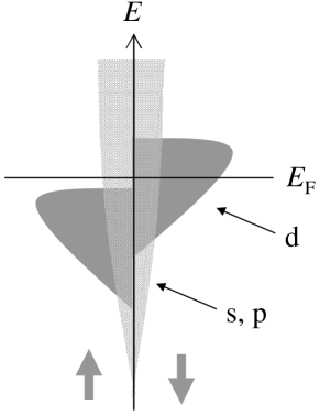
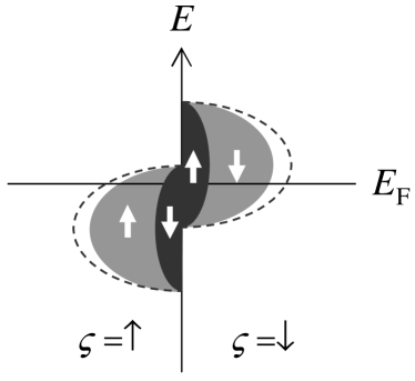
where () represents a resistivity for the case of the electrical current parallel to the magnetization (a resistivity for the case of the current perpendicular to the magnetization). Table 1 shows the experimental values of the AMR ratios of typical ferromagnets, i.e., body-centered cubic (bcc) Fe[8] face-centered cubic (fcc) Co,[8] fcc Ni,[8] Fe4N,[16, 17] and the half-metallic ferromagnet.[11, 12, 13, 14, 15] Here, bcc Fe is categorized as a weak ferromagnet,[21] in which its majority-spin d band is not filled (see Fig. 1(a)). In contrast, fcc Co, fcc Ni, and Fe4N are strong ferromagnets,[21] in which their majority-spin d band is filled (see Fig. 1(b)). In addition, the half-metallic ferromagnet is defined as having a finite density of states (DOS) at the Fermi energy in one spin channel and a zero DOS at in the other spin channel (see Figs. 1(d) and 1(e)). As remarkable points, Fe,[8] Co,[8] and Ni[8] exhibited positive AMR ratios, while Fe4N[16, 17] and the half-metallic ferromagnets[11, 12, 13, 14, 15] showed negative AMR ratios. Furthermore, in the case of Fe3O4[12, 13] of the half-metallic ferromagnet, the sign of the AMR ratio changed from negative to positive with increasing temperature. For such ferromagnets, however, theoretical studies to systematically explain their AMR ratios have been scarce so far. In particular, a feature that strongly affects the sign of the AMR ratio has not yet been revealed.
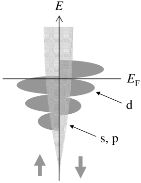
(a) bcc Fe
(b) fcc Co and fcc Ni

(c) Fe4N
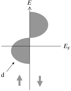

(d) Half-metallic ferromagnet (e) Fe3O4 (half-metallic ferromagnet)
| Category | Material | AMR ratio (experimental value) | ||
|---|---|---|---|---|
| Weak ferromagnet[21] | bcc Fe | 0.0030 at 300 K (ref. \citenMcGuire) | 3.8 10-1 (ref. \citenTsymbal) | 2.0 (ref. \citenWang) |
| Strong ferromagnet[21] | fcc Co | 0.020 at 300 K (ref. \citenMcGuire) | 7.3 (ref. \citenTsymbal) | (ref. \citenMatar) |
| fcc Ni | 0.022 at 300 K (ref. \citenMcGuire) | 1.0 10 (ref. \citenKokado_un1) | (ref. \citenVargas) | |
| Fe4N | 0.043 - 0.005 for 4.2 K - 300 K (ref. \citenTsunoda) | 1.6 10-3 (ref. \citenKokado_un) | 0.2 (ref. \citenSakuma) | |
| 0.07 - 0.005 for 4 K - 300 K (ref. \citenTsunoda1) | ||||
| Half-metallic ferromagnet | Co2MnAl1-xSix | 0.003 - 0.002 at 4.2 K (ref. \citenEndo) | ||
| La0.7Sr0.3MnO3 | 0.0015 at 4 K (ref. \citenFavre) | |||
| La0.7Ca0.3MnO3 | 0.0012 at 75 K (ref. \citenZiese) | |||
| 0.004 at 100 K (ref. \citenZiese1) | ||||
| Fe3O4 | 0.005 - 0.005 for 100 K - 300 K (refs. \citenZiese and \citenZiese2) |
Theoretically, expressions of the AMR ratio have been derived by taking into account a resistivity due to the s–d scattering.[1, 3, 4, 7, 9, 10, 12, 18] This scattering represents that the conduction electron is scattered into the localized d states by impurities. The d states have exchange field and spin–orbit interaction, i.e., , where is the spin–orbit coupling constant, (=, , ) is the orbital angular momentum, and (=, , ) is the spin angular momentum. Here, the d states are spin-mixed owing to the spin–orbit interaction.
The applicable scope of the previous theories, however, appears to be limited to specific materials because only the partial components in the whole resistivities have been adopted. For example, Campbell, Fert, and Jaoul[3] (CFJ) derived an expression of the AMR ratio of a strong ferromagnet[9] such as Ni-based alloys, i.e.,[19]
| (2) |
with and .[20] Here, was a resistivity of the conduction state (named as ) of the spin, with or . In addition, was a resistivity due to the s–d scattering, in which the conduction electron was scattered into the localized d states of the spin by impurities. The spin represented the spin of the dominant state in the spin-mixed state, where the up spin () and down spin () meant the majority spin and the minority spin, respectively. Note that the CFJ model adopted only and on the basis of scattering processes between the dominant states at . The processes were , , and ,[3] where represented the scattering process between the conduction states of the spin, while was the scattering process from the conduction state of the spin to the spin state in the localized d states of the spin. On the other hand, Malozemoff[9, 10] extended the CFJ model to a more general model which was applicable to the weak ferromagnet as well as the strong ferromagnet. This model took into account , , , and on the basis of the scattering processes of , , , , , and . In the actual application to materials, however, he often used an expression of the AMR ratio with , [9, 10] i.e.,
| (3) |
which was always positive. Equation (3) was an expression for the weak ferromagnet, while Eq. (3) with was that for the strong ferromagnet.
Furthermore, we point out a problem, namely, that the previous theories have not taken into account the spin dependence of the effective mass and the number density of electrons in the conduction band in expressions of the resistivities. For example, the half-metallic ferromagnets which have the DOS’s of Figs. 1(d) and 1(e) may show significant spin dependence.
On the basis of this situation, we suggest improvements for a systematic analysis of the AMR effects of various ferromagnets. First, the expression of the AMR ratio should treat as a variable. The reason is that actually depends strongly on the materials (see Table 1). Namely, has been evaluated to be 3.8 10-1 for bcc Fe,[22] 7.3 for fcc Co,[22] 1.0 10 for fcc Ni,[23, 24] and 1.6 10-3 for Fe4N,[25, 26] from analyses using a combination of the first principles calculation and the Kubo formula within the semiclassical approximation. The half-metallic ferromagnet is also assumed to have or . It is noteworthy here that the conduction state (called in suffixes of ) is considered to consist of not only the s and p states but also the conductive d state. In addition, the exchange splitting of the s and p states is attributed to the fact that the s and p states are coupled to the d states with exchange splitting through the transfer integrals. Second, in the case of the half-metallic ferromagnet, the expressions of the resistivities should take into account the spin dependence of the effective mass and the number density of the electrons in the conduction band.
In this paper, we first derived general expressions of the resistivities and the AMR ratio. We here treated as a variable and took into account the spin dependence of the effective mass and the number density of the electrons in the conduction band. Second, on the basis of the expressions, we roughly determined a relation between the sign of the AMR ratio and the dominant s–d scattering process. Namely, when the dominant s–d scattering process was or , the AMR ratio tended to become positive. In contrast, when the dominant s–d scattering process was or , the AMR ratio tended to be negative. Finally, using the expression of the AMR ratio, we systematically analyzed the AMR ratios of Fe, Co, Ni, Fe4N, and the half-metallic ferromagnet. The evaluated AMR ratios corresponded well with the respective experimental results. In addition, the sign change of the AMR ratio of Fe3O4 could be explained by considering the increase of the majority spin DOS at .
The present paper is organized as follows: In §2, we derive general expressions of the resistivities and the AMR ratio. We then find the relation between the sign of the AMR ratio and the s–d scattering process. In §3 and §4, from the general expression, we obtain expressions of AMR ratio appropriate to the respective materials. Using the expressions, we analyze their AMR ratios. Concluding remarks are presented in the §5. In the Appendix A, we obtain wave functions of the localized d states (i.e., the spin-mixed states) from a single atom model that involves the spin–orbit interaction. In Appendixes B and C, we derive expressions of s–d and s–s scattering rates, respectively. In the Appendix D, we show matrix elements in the s–d scattering rate. Some parameters are formulated in the Appendix E.
2 Theory
We derive general expressions of resistivities due to electron scattering by nonmagnetic impurities and then obtain a general expression of the AMR ratio. On the basis of the resistivities and the AMR ratio, we explain a feature of the AMR effect. In addition, we find a relation between the sign of the AMR ratio and the scattering process.
2.1 Model
Following the Smit model[1] and the CFJ model[3], we use a simple model consisting of the conduction state and the localized d states. The conduction state is represented by a plane wave, while the localized d states are described by a tight-binding model, i.e., the linear combination of atomic d orbitals.[3] The d orbitals are obtained by applying a perturbation theory to a Hamiltonian for the d electron in a single atom, :
| (6) | |||||
Here, the unperturbed term is the Hamiltonian for the hydrogen-like atom with Zeeman interaction due to , where is the exchange field of the ferromagnet, is the electron mass, and is the Planck constant divided by 2. The term is a spherically symmetric potential energy of the d orbitals created by a nucleus and core electrons, with , where is the position vector. The perturbed term is the spin–orbit interaction with . Here, the azimuthal quantum number and the spin quantum number are chosen to be =2 and =1/2, respectively. From this model, we obtain the spin-mixed states within the second-order perturbation (see Appendix A).
2.2 Resistivity
Using the localized d states and the conduction state, we can obtain the resistivity for the case of a parallel () or perpendicular () configuration. As a starting point, we consider the two-current model[27] composed of the up spin and down spin current components. In addition, this model is improved by including the spin-flip scattering, which is due to, for example, spin-dependent disorder[28, 29] and magnon[30, 31]. The resistivity of configuration ( or ) is then written as[32]
| (7) |
with
| (8) | |||
| (9) | |||
| (10) |
where is a resistivity of the spin state for the configuration,[33, 34, 35, 36, 37, 31, 18] while () is a resistivity due to the spin-flip scattering process from the spin state to the spin state for the configuration. It is noted that eq. (7) with =0 corresponds to the resistivity of the two-current model. The constant is the electronic charge, and () is the number density[34, 35] (the effective mass[38]) of the electrons in the conduction band of the spin, where the conduction band consists of the s, p, and conductive d states. The quantity is a relaxation time of the conduction electron of the spin for the configuration, and is a relaxation time of the spin-flip scattering process from the spin state to the spin state for the configuration. The scattering rate is expressed as[5, 4]
| (11) |
Here, is a relaxation time of the conduction state of the spin, where this state consists of the s, p, and conductive d states. In addition, is a relaxation time of the s–d scattering for the configuration. This s–d scattering means that the conduction electron of the spin is scattered into “the spin state in the localized d state of and ” by nonmagnetic impurities. The quantities (, 1, 0, 1, 2) and ( or ) are, respectively, the magnetic quantum number and the spin of the dominant state in the spin-mixed state (see Appendix A). The expressions of and are derived in Appendixes B and C, respectively.
Using eqs. (92), (65) - (74), and (D) - (D), we obtain of eq. (8) as
| (12) | |||
| (13) | |||
| (14) | |||
| (15) |
with
| (16) | |||
| (17) | |||
| (18) | |||
| (19) | |||
| (20) | |||
Here, terms higher than the second order of have been ignored. Accordingly, terms with in eqs. (12) - (2.2) correspond to terms obtained from only the Smit[1] spin-mixing mechanism[7, 10] with (see Appendix A). In contrast, terms related to the operator have been eliminated. A resistivity of the conduction state of the spin, , is due to the s–s scattering, in which the conduction electron of the spin is scattered into the conduction state of the spin by nonmagnetic impurities (see Appendix C). In addition, is a resistivity due to the s–d scattering. The s–d scattering means that the conduction electron of the spin is scattered into “the spin state in the localized d state of and ” by the impurities, where and are as explained above (see Appendixes A and B). The quantities and are the relaxation times of the s–s and s–d scatterings, respectively. The quantity is the matrix element of the impurity potential for the s–s scattering (see eq. (97)), while is that for the s–d scattering (see eqs. (B), (92), and (75), and Appendix D), where is the Fermi wavevector of the spin in the current direction. Here, each impurity is assumed to have a spherically symmetric scattering potential which acts only over a short range. The quantity is the DOS of the conduction state of the spin at (see eq. (98)), and is that of the d state of and at (see eq. (93)). Furthermore, is the impurity density, and is the number of the nearest-neighbor host atoms around the impurity (see eq. (B)).
| Summation | ||||
|---|---|---|---|---|
When the dependence of in eq. (20) is ignored in a conventional manner,[3] eqs. (12) - (2.2) become
| (22) | |||
| (23) | |||
| (24) | |||
| (25) |
respectively, with
| (26) | |||
| (27) |
where , , and are given by eqs. (16), (17), and (2.2), respectively. Here, is the DOS of each d state of the spin at , where is set to be by ignoring for of eq. (93).
2.3 AMR ratio
Using eqs. (1), (7), and (22) - (25), we obtain the general expression of the AMR ratio as
| (28) |
with
| (29) | |||
| (30) | |||
| (31) | |||
| (32) | |||
| (33) |
where () is a resistivity due to the spin-flip scattering process from the spin state to the spin state, and is a relaxation time of this scattering. Here, has been assumed to be independent of the configuration (see of eq. (9)).
2.4 Feature of the AMR effect
On the basis of the above results, we introduce a certain quantity based on the AMR ratio and then reveal a feature of the AMR effect. In particular, we find that the sign of the AMR ratio is determined by the increase or decrease of “existence probabilities of the specific d orbitals” due to the spin–orbit interaction. In addition, we roughly determine a relation between the sign of the AMR ratio and the scattering process.
2.4.1
Taking into account the after-mentioned (i) - (iii), we introduce the quantity based on the AMR ratio. Here, the AMR ratio reflects the difference of “changes of the d orbitals due to the spin–orbit interaction” between different ’s, where is the magnetic quantum number of the d orbital of eq. (75). Such a quantity is written as
| (34) | |||
| (35) | |||
| (36) |
where is given by eqs. (65) - (74). Roughly speaking, may correspond to the numerator of the AMR ratio of eq. (1), . In particular, in and in may be related to and , respectively. This represents the change of “the existence probability of the d orbital of and ” due to the spin–orbit interaction. Here, is adopted on the basis of the scattering rate in (see Appendix B), and comes from that in the right-hand side of eq. (11). In addition, 1/4, 3/8, and 3/8 in correspond to the coefficients of of eq. (2.2) in the scattering rates of =0, 2, and 2, respectively (see Appendix D). Such and have been based on the following (i) - (iii):
-
(i)
By comparing eqs. (22) and (24) or eqs. (23) and (25), we find that the AMR effect arises from the difference of s–d scattering terms between and configurations. All the s–d scattering terms with in eqs. (22) - (25) are listed in Table 2, where terms with in eqs. (12) - (2.2) are also listed. The s–d scattering terms in originate from a transition from the plane wave to the d orbital of =0, (see Appendix D).[3] In contrast, the s–d scattering terms in are due to transitions from the plane wave to the d orbitals of and 0, and . The d orbitals of , , give no contribution to and .
- (ii)
-
(iii)
The terms stem from the change of the d orbitals due to the spin–orbit interaction. The d orbital is slightly changed by the spin-mixing term in the spin–orbit interaction. It is noteworthy that the contributions due to the term are eliminated by ignoring terms higher than the second order of (see Appendix A).
| (, ) | (, ) | (, ) | (, ) | (, ) |
|---|---|---|---|---|
| 0 | 0 | |||
| 0 | 0 | |||
2.4.2 Sign of and s–d scattering
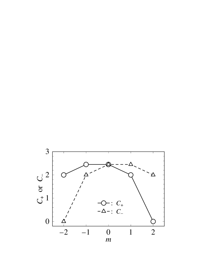
In order to obtain , we first investigate of eq. (36). As seen from Table 3, , , , and become negative, while , , , and are positive. Here, the former ’s are obtained from the first terms in the right-hand sides of eqs. (65) - (68) and (71) - (74). The latter ’s are obtained from the second terms in them. The negative sign of the former means that the existence probability of the pure d orbital of decreases owing to hybridization with the other d orbital in the presence of the spin–orbit interaction (see the gray areas in Fig. 2(b)). In contrast, the positive sign of the latter represents the addition of the existence probability of the other d orbital (see the black areas in Fig. 2(b)). Note that the spin of the other d orbital is opposite to that of the pure d orbital under the influence of in the spin-mixing term.
Furthermore, we find a relation of for each set of and . The relation is attributed to the mixing effect of the d orbitals due to in the spin-mixing term. This effect is verified from the dependence of (=) in Fig. 3, where = and =2. The coefficient at becomes larger than that at ; that is, the mixing effect at is larger than that at .
Using such ’s, we can obtain of eq. (34) as shown in Table 3. In addition, we find the following relation between the sign of and the s–d scattering process : for , for , for , and for (see Table 3). Here, indicates that the conduction electron of the spin is scattered into in of - 2. The spin is conserved in the scattering process. The spins and of are extracted from . Roughly speaking, the negative sign of and originates from the decrease of the existence probability of the pure d orbital, while the positive sign of and is due to the addition of the existence probability of the other d orbital (see Fig. 2(b)).
Since may correspond approximately to of the AMR ratio, we can roughly determine the relation between the sign of the AMR ratio and the s–d scattering process. Namely, when the dominant s–d scattering process is or , the AMR ratio tends to become negative. In contrast, when the dominant s–d scattering process is or , the AMR ratio tends to be positive. Such a relation agrees with a trend for real materials, as will be shown in §2.5.
(a) (b)
2.5 Sign of the AMR ratio and s–d scattering of real material
Within a unified framework, we find the sign of the AMR ratio and the dominant scattering process of each material in Table 1. We here utilize and from Table 1.
2.5.1 A simple model
Toward the unified framework, we present a simple model with (), , , and =0. This model has a relation of from eqs. (22) - (25). The AMR ratio of eq. (1) is then expressed as
| (37) |
Using eqs. (22) - (27), eq. (37) is rewritten as
| (38) | |||
| (39) | |||
| (40) |
with
| (41) |
where is given by eq. (17), and is written by eq. (26) with . This corresponds approximately to the resistivity of the spin for a system with no spin–orbit interaction, i.e., eqs. (22) - (25) with =0. Note here that in in eq. (41) actually contains the effect of the spin–orbit interaction, as found from eq. (93).
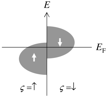
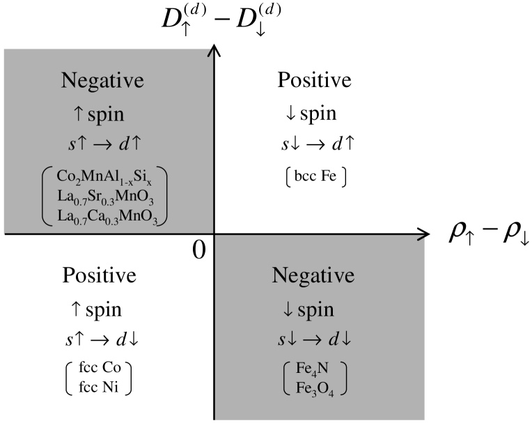
From eqs. (38) - (40), we can find the relation between the sign of the AMR ratio and the dominant s–d scattering process. First, the sign of the AMR ratio is shown in each quadrant of the - plane of Fig. 4. The AMR ratio becomes positive in the case of and or in the case of and . In contrast, the AMR ratio is negative in the case of and or in the case of and . Here, the case of () shows that the down spin electrons (the up spin electrons) contribute dominantly to the transport. Furthermore, the dominant s–d scattering process is indicated by in each quadrant of Fig. 4. The process is extracted from , which contributes dominantly to the sign of the AMR ratio. Concretely speaking, this corresponds to the greater of and in the case of and the greater of and in the case of . It is also noteworthy that the relation in Fig. 4 is consistent with the result in §2.4.2 or Table 3.
2.5.2 Application to materials
Applying and of Table 1 to the results of Fig. 4, we can roughly determine the dominant s–d scattering and the sign of the AMR ratio of each material. The determined signs agree with the experimental results of Table 1. The details are written as follows:
-
(i)
bcc Fe
The dominant s–d scattering is because of and . The AMR ratio is thus positive. Here, originates from and due to . -
(ii)
fcc Co and fcc Ni
The dominant s–d scattering is because of and . The AMR ratio is then positive. Here, is obtained from and due to . -
(iii)
Fe4N
The dominant s–d scattering is because of and . The AMR ratio is thus negative. Here, mainly results from (see Table 1). The relation =0 is assumed by considering that is considerably smaller than , where it is reported that this model has . In addition, we assume that , which will be estimated in §3.3. -
(iv)
Co2MnAl1-xSix, La0.7Sr0.3MnO3, and La0.7Ca0.3MnO3
The dominant s–d scattering is because of and . The AMR ratio is thus negative. Here, mainly originates from (see (i) of §4.1 or §4.3). The relation =0 is roughly set on the basis of , where . In addition, we assume that , which will be estimated in §4.3. -
(v)
Fe3O4
The dominant s–d scattering is because of and . The AMR ratio is then negative. Here, mainly stems from (see (i) of §4.1 or §4.3). The relation =0 is roughly set on the basis of , where . In addition, we assume that , which will be estimated in §4.3. Note that, in this system, the direction of each spin in (iv) has been reversed by taking into account the DOS of Fig. 1(e).
3 Application 1: Weak or Strong Ferromagnet
On the basis of the theory of §2, we obtain the expressions of the AMR ratios of “bcc Fe of the weak ferromagnet” and “fcc Co, fcc Ni, and Fe4N of the strong ferromagnet.” Using the expressions, we analyze their AMR ratios.
3.1 AMR ratio
From eq. (28), we first derive an expression of the AMR ratio of the weak or strong ferromagnet. The weak or strong ferromagnet has the sp band DOS of the up and down spins at (see Figs. 1(a), 1(b), and 1(c)). We thus use the conventional approximation in order to reduce parameters. Namely, we set , , , and . Meanwhile, the dependence of and the dependence of are taken into account (see eqs. (17), (19), (26), and (27)). The AMR ratio of eq. (28) is then given simply by
where
| (43) | |||
| (44) |
Here, we have , , and , where and . In addition, of eq. (33) is rewritten by . It is noteworthy that has no influence on the sign of the AMR ratio of eq. (3.1). Also, eq. (3.1) with =0 corresponds to an expression of the AMR ratio obtained by Malozemoff.[9]
3.2 Weak ferromagnet: Fe
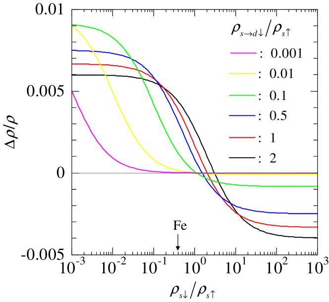
Using eq. (3.1), we analyze the AMR ratio of bcc Fe of the weak ferromagnet. Here, (=) is assumed to be =2.0 on the basis of =2.0 of Table 1.[39] The constant is chosen to be =0.01 as a typical value. Meanwhile, we ignore which does not change the sign of the AMR ratio. It is noteworthy that the spin-dependent disorder[28, 29], which gives rise to the spin-flip scattering, may be weak for the present ferromagnets with nonmagnetic impurities.
In Fig. 5, we show the dependence of the AMR ratio for any . The AMR ratio behaves as a smooth step-like function. In addition, the AMR ratio tends to be positive for or negative for . In the case of =3.8 of Table 1, the AMR ratio becomes positive irrespective of . In particular, when =0.5, the AMR ratio agrees fairly well with the experimental value, i.e., 0.003.
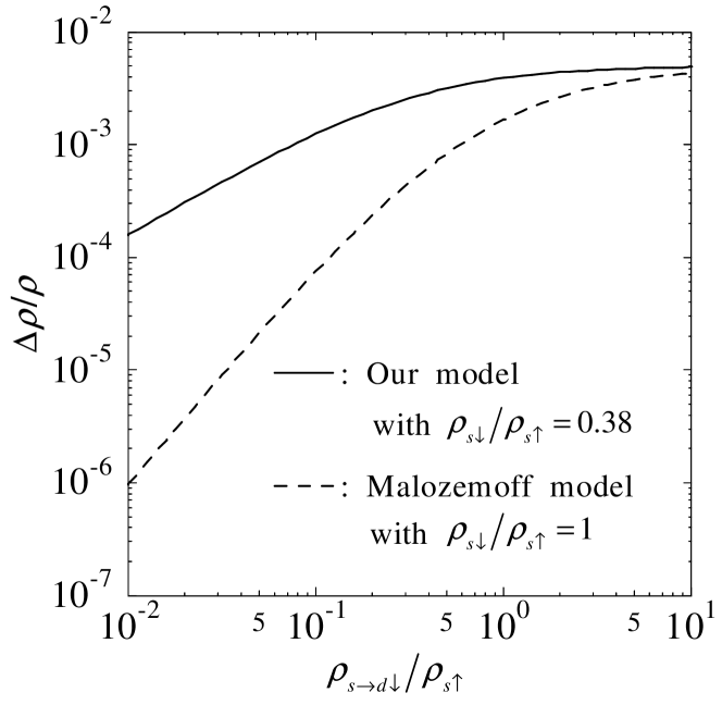
Figure 6 shows the dependence of the AMR ratio. Our model with =3.8 is compared with the Malozemoff model with =1,[9] i.e., eq. (3). The difference of the AMR ratio between them becomes prominent for . For example, in the case of the above-mentioned =0.5, the AMR ratio of our model is about four times as large as that of the Malozemoff model.
3.3 Strong ferromagnet: Co, Ni, and Fe4N
Utilizing eq. (3.1), we investigate the AMR ratios of fcc Co, fcc Ni, and Fe4N of the strong ferromagnet. The DOS of this system is schematically illustrated in Figs. 1(b) and 1(c). The fcc Co[40] and fcc Ni[41, 24] have little d band DOS of the up spin at . As to Fe4N,[42] the d band DOS of the up spin is considerably smaller than that of the down spin at . We thus assume =0 and then have =0. Substituting =0 into eq. (3.1), we obtain the AMR ratio as
| (45) |
Here, when is sufficiently small or sufficiently large, eq. (45) with =0 is approximated as
| (48) |
where is set to be in the present calculation. The respective expressions of eq. (48) increase with increasing and , while the magnitude of the difference between the two expressions is given by . We also mention that corresponds approximately to the CFJ model[3] of eq. (2), which is applicable to the strong ferromagnet. Here, in eq. (2) is originally defined by (see eqs. (24) and (25)). This can be rewritten as under the following conditions: One is the condition of the CFJ model, i.e., , , , and . The other is the condition of . The latter reflects that =0.01 and are set in the present study (see Figs. 7 and 8).
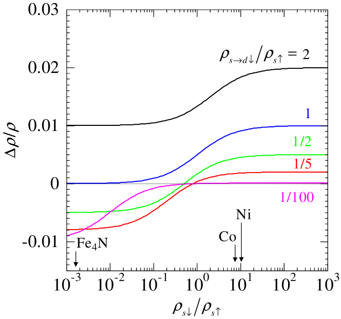
In Fig. 7, we show the dependence of the AMR ratio of eq. (45) with =0. The quantity is chosen to be =0.01 as a typical value. We find that the AMR ratio behaves as a smooth step-like function with the limiting values of eq. (48). In particular, the AMR ratio is positive for , while it can be negative for and . Note that the system of corresponds to Co and Ni, while that of corresponds to Fe4N.
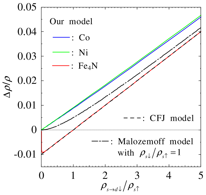
When ’s of Co, Ni, and Fe4N are respectively set to be 7.3, 1.0, and 1.6 of Table 1, we obtain the dependence of the AMR ratios as shown in Fig. 8. The main results are as follows:
-
(i)
The fcc Co and fcc Ni exhibit a positive AMR ratio irrespective of , while Fe4N can take the negative AMR ratio depending on . Such tendencies roughly correspond to the experimental results (see Table 1). On the basis of the experimental values of the AMR ratios, ’s of Co, Ni, and Fe4N are evaluated to be , , and , respectively. It is noted here that the large AMR ratio of Fe4N (e.g., 0.07) cannot be obtained in the present theory. Eventually, a theoretical model that takes into account a realistic band structure may be necessary for a quantitative analysis.[43]
-
(ii)
The AMR ratios calculated for fcc Co and fcc Ni are clearly different from the CFJ model of eq. (2) because ’s of Co and Ni are largely different from that in the CFJ model (i.e., ). In contrast, the AMR ratio calculated for Fe4N agrees well with the CFJ model, because (=1.6 10-3) of Fe4N is much smaller than 1.
-
(iii)
The AMR ratios calculated for fcc Co, fcc Ni, and Fe4N deviate from the Malozemoff model with =1, i.e., eq. (3). The reason is that their ’s are different from 1.
4 Application 2: Half-Metallic Ferromagnet
On the basis of the theory of §2, we derive an expression of the AMR ratio of the half-metallic ferromagnet. Using the expression, we obtain an accurate condition for the negative or positive AMR ratio and further analyze the AMR ratio.
4.1 AMR ratio
We first report the feature of the half-metallic ferromagnet of Table 1. The DOS of Co2MnAl1-xSix,[44] La0.7Sr0.3MnO3,[45, 46] or La0.7Ca0.3MnO3[47] is schematically illustrated in Fig. 1(d). The conductive and localized d band DOS’s of the up spin are present at , while there is little DOS of the down spin. In real systems, however, there may be a slight DOS of the down spin in the presence of disorders or defects. According to previous studies, such a feature of the DOS of Co2MnAl1-xSix originates from atomic disorders,[48] while that of La0.7Sr0.3MnO3[49, 50] or La0.7Ca0.3MnO3 may be due to oxygen vacancies.[51] It is also noted that, by reversing the direction of each spin, we can treat the opposite case (i.e., Fe3O4[52, 53] of Fig. 1(e)), in which the DOS of the down spin is present at , while there is little DOS of the up spin.
Focusing on the half-metallic ferromagnet with the DOS of Fig. 1(d), we now obtain an expression of the AMR ratio as accurately as possible. We here utilize the AMR ratio of eq. (28) because and are considered to have the significant dependence. Meanwhile, and are ignored in the same manner as in §3.2. The AMR ratio of eq. (28) with is rewritten as
| (49) |
with
| (50) | |||
| (51) | |||
| (52) | |||
| (53) | |||
| (54) | |||
| (55) |
where eq. (50) has been derived in the Appendix E and eqs. (51) - (54) have been obtained by using eqs. (17), (19), (26), and (27). We also have assumed and on the basis of the above-mentioned feature of the DOS of the down spin. Here, the conduction state (named as in ) may correspond to the conductive d state in the case of the present half-metallic ferromagnet (see Figs. 1(d) and 1(e)). From eqs. (51) - (54), we find the following relation:
| (56) |
Using this relation, we express eq. (49) as
| (57) |
Here, parameters in eq. (57), , , , and , are suggested as follows:
-
(i)
The parameter of eq. (50) may become extremely large owing to . This relation is based on the fact that the resistivity of semiconductors is more than 104 times larger than that of metals.[54] As a typical system, we consider to be on the assumption of and . Here, has been roughly estimated on the basis of the effective mass of the carrier of the semiconductor divided by the electron mass.[54]
-
(ii)
The parameter of eq. (52) takes a finite value, where and . In the present calculation, is treated as a variable number of .
-
(iii)
The parameter of eq. (53) may be sufficiently large because of . In the case of the reported above, we find the relation of , where has been assumed.
-
(iv)
The parameter of eq. (54) may take a finite value, although both and are extremely small. In addition, the relation of is realized.
On the basis of eqs. (50) - (54) and the above suggestions, we next obtain an approximate expression of eq. (57). We here assume and and also take into account in (iv), , and , where and in (i) have been adopted. Equation (57) has thus been written as
| (58) |
The AMR ratio of eq. (58) always takes a negative value.
4.2 Sign of AMR ratio
From eq. (57), we can find the condition for the negative or positive AMR ratio of the half-metallic ferromagnet. This condition is more accurate than the result in the unified framework of §2.5. Because of in (iv), we focus on the numerator in of eq. (57). The numerator is written by with
| (59) | |||
| (60) |
where and . Here, and correspond to the negative and positive AMR ratios, respectively. From eq. (59), we first find that the AMR ratio becomes positive when . Second, in the case of , the AMR ratio is negative for
| (61) |
while it is positive for
| (62) |
with and . Note that the AMR ratio becomes 0 at .
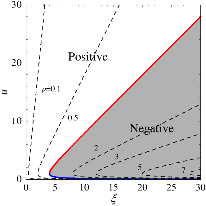
Figure 9 shows the sign of the AMR ratio in the - plane based on the above results. From this figure, we can find signs of the AMR ratios of various systems. We here focus on a simple system with and (i.e., ). For this system, we first determine the specific sets of and . The relation between and has been obtained as
| (63) |
with (see eq. (107)). In Fig. 9, we show eq. (63) with =0.1, 0.5, 2, 3, 5, and 7 by the dashed curves, where eq. (63) with =1 corresponds to and . It is found that eq. (63) with 1 exists in the region of the negative AMR ratio. For example, the case of and in (i) leads to . This case thus can take the negative AMR ratio. Negative AMR ratios been experimentally observed, as shown in Table 1.
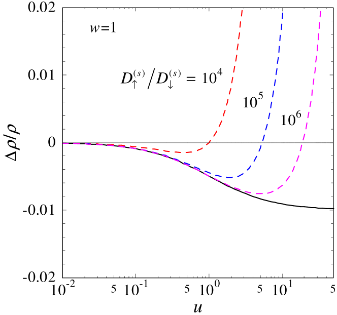
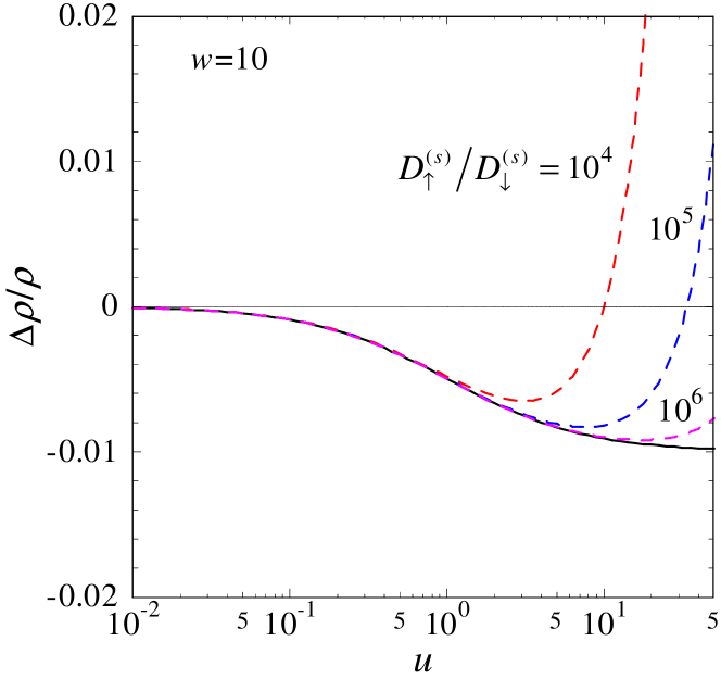
4.3 Evaluation of AMR ratio
Using the results of §4.1 and §4.2, we evaluate the AMR ratio. The dependence of the AMR ratio is shown in Fig. 10. The dashed curves represent eq. (57) with the parameters of =0.01, , , , =1, 10, and =104, 105, 106, where =0.1 and . The parameters have been chosen on the basis of (i) - (iv) in §4.1. We observe that each AMR ratio exhibits a convex downward curve with a negative minimum value. The AMR ratio approaches 0 with decreasing , while it changes from negative to positive with increasing . In addition, the AMR ratio comes close to eq. (58) with =0.01 (the solid curve) with increasing . It is noted that eq. (58) is obtained from eq. (57) under the condition of , , and in (iv). Also, in the case of , the AMR ratio becomes about 0.004 at (see the upper panel of Fig. 10), where the system of corresponds to the simple system in §4.2. This AMR ratio agrees well with the experimental results of Table 1.
4.4 Sign change of the AMR ratio in Fe3O4
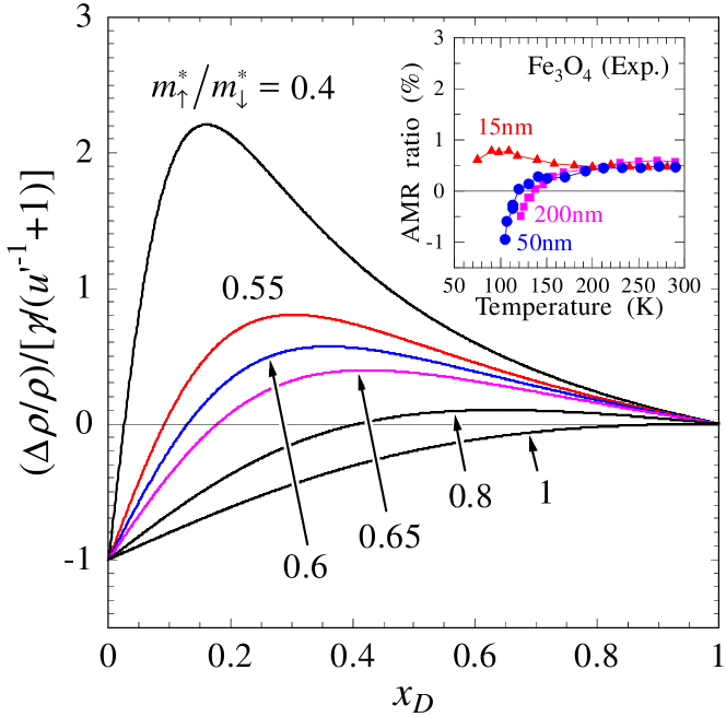
Utilizing eq. (57), we analyze an experimental result of Fe3O4, in which the sign of the AMR ratio changes from negative to positive as the temperature increases.[12, 13] Here, Fe3O4 has been theoretically predicted to have a half-metallic property at the ground state in the absence of the spin–orbit interaction.[53] The DOS of Fe3O4 is schematically illustrated in Fig. 1(e):[52, 53] the DOS of the down spin is present at , while there is little DOS of the up spin.
Recently, Ziese has experimentally observed that the Fe3O4 film on MgO with film thickness of 50 nm or 200 nm changed the sign of the AMR ratio from negative to positive with increasing temperature (see the inset of Fig. 11).[12, 13] This Fe3O4 eventually exhibited positive AMR ratios of about 0.005 at temperatures higher than 200 K. As a cause of this phenomenon, he considered that the majority spin band (i.e., band) came close to with increasing temperature, and, furthermore, this band was present at in the high temperature region (e.g., the region higher than 200 K). On the basis of such an idea, he proposed a two-band model composed of and bands; and bands have been shown in Fig. 1(e). Using the model, he primarily found that the AMR ratio became 0.005 for the specific values of the minority-to-majority resistivity ratio and the reduced spin-flip scattering resistivity. Meanwhile, he also showed that the sign of the AMR ratio changed from negative to positive with increasing .[55] Here, is reduced to in our formulation (see eq. (44)). From the standpoint of the AMR ratio versus , however, we see a problem; that is, the sign change of this model appears to be contrary to the experimental trend of the inset of Fig. 11 or the above idea. In fact, with decreasing , the sign may change from negative to positive. In addition, we notice that this model consists of only the resistivities due to the s–d scattering but neglects the resistivity of the conductive d states, , due to the scattering process between the conductive d states.[56] For this situation, we believe that there is a need to reexamine the sign change of the AMR ratio by using a model that takes into account both resistivities.
We, therefore, demonstrate the sign change of the AMR ratio using our model with both resistivities. On the basis of the behavior of the band reported above, we assume that the DOS of the up spin at increases with increasing temperature. Our concern, thus, is with how the DOS of the up spin influences the AMR ratio. To clearly show the influence, we consider a simple case of (or ) and . By paying attention to the DOS of Fig. 1(e), i.e., the reversion of the direction of each spin of eq. (57), eq. (57) is then rewritten as
| (64) |
with and =. Figure 11 shows the dependence of the AMR ratio of eq. (64) for =0.4, 0.55, 0.6, 0.65, 0.8, and 1. The AMR ratios of =0.4, 0.55, 0.6, 0.65, and 0.8 change from negative to positive with increasing , although that of =1 is always negative. The sign change appears to originate from the feature in which the s–d scatterings of and increase with increasing and . Here, it is noteworthy that these s–d scatterings tend to lead to the positive AMR ratio (see §2.4 and §2.5). In addition, roughly speaking, the dependence of the AMR ratio appears to be qualitatively similar to the experimental trend of the inset of Fig. 11. In particular, the AMR ratios of =0.6 and 0.65 may correspond well to the experimental results for film thicknesses of 50 nm and 200 nm, respectively. In addition, the AMR ratio of =0.55 may partially correspond to the experimental result for film thicknesses of 15 nm.
5 Conclusion
We systematically analyzed the AMR effects of bcc Fe of the weak ferromagnet, fcc Co, fcc Ni, and Fe4N of the strong ferromagnet, and the half-metallic ferromagnet. We here used the two-current model for a system consisting of a spin-polarized conduction state and localized d states with spin–orbit interaction.
From such a model, we first derived general expressions of resistivities composed of and . The resistivity arose from the s–s scattering, in which the conduction electron of the spin was scattered into the conduction state of the spin by nonmagnetic impurities. The resistivity was due to the s–d scattering, in which the conduction electron of the spin was scattered into the spin state in the localized d states of the spin by the impurities, where the spin represented the spin of the dominant state in the d states (i.e., the spin-mixed states).
Using the resistivities, we next obtained a general expression of the AMR ratio. On the basis of the AMR ratio and the resistivities, we showed that the AMR effect reflected the difference of “changes of the d orbitals due to the spin–orbit interaction” between different ’s, where was the magnetic quantum number of the d orbital. In addition, we roughly determined a relation between the sign of the AMR ratio and the scattering process. In brief, when the dominant s–d scattering process was or , the AMR ratio tended to become positive. In contrast, when the dominant s–d scattering process was or , the AMR ratio tended to be negative.
Finally, from the general expression of the AMR ratio, we obtained expressions of AMR ratios appropriate to the respective materials. Using the expressions, we analyzed their AMR ratios. The results for the respective materials were written as follows:
-
(i)
bcc Fe of weak ferromagnet
Using the AMR ratio of eq. (3.1) with in Table 1 and =0, we found that the AMR ratio became positive irrespective of , where has been set. In particular, when =0.5, the AMR ratio agreed fairly well with the experimental value in Table 1, i.e., 0.003. Here, the positive AMR ratio originated from the dominant s–d scattering process of . Regarding the dependence of the AMR ratio, the difference of the AMR ratio between our model with =3.8 and the Malozemoff model with =1 was clearly observed for . -
(ii)
fcc Co, fcc Ni, and Fe4N of strong ferromagnet
Using the AMR ratio of eq. (45) with =0 and ’s in Table 1, i.e., 7.3 for fcc Co, 1.0 for fcc Ni, and 1.6 for Fe4N, we found that fcc Co and fcc Ni exhibited a positive AMR ratio irrespective of , while Fe4N could take the negative AMR ratio depending on . In particular, when ’s of fcc Co, fcc Ni, and Fe4N were, respectively, chosen to be 2.2, 2.5, and , their AMR ratios corresponded well to the respective experimental values in Table 1, i.e., 0.020 for fcc Co, 0.022 for fcc Ni, and 0.01 - 0.005 for Fe4N. It is noted, however, that the large AMR ratio of Fe4N (e.g., 0.07 - 0.02) could not be obtained in the present theory. The positive AMR ratios of fcc Co and fcc Ni originated from the dominant s–d scattering process of . In contrast, the negative AMR ratio of Fe4N was due to the dominant s–d scattering process of . As for the dependence of the AMR ratios, the calculation result of fcc Co and fcc Ni by our model was obviously different from those by the CFJ model and the Malozemoff model. The reason was that () of fcc Co or fcc Ni was largely different from (1) of the CFJ model and (=1) of the Malozemoff model. In the case of Fe4N, the result by our model agreed well with that by the CFJ model because (=1.6 10-3) of Fe4N corresponded well to (1) of the CFJ model. -
(iii)
half-metallic ferromagnet
Using the AMR ratio of eq. (57), which took into account the spin dependence of the effective mass and the number density of electrons in the conduction band, we showed that the AMR ratio could become negative for a typical system with and . In particular, when , the AMR ratio was evaluated to be about 0.004, which was close to the experimental values. Here, the negative AMR ratio of Co2MnAl1-xSix, La0.7Sr0.3MnO3, and La0.7Ca0.3MnO3 originated from the dominant s–d scattering process of , while the negative AMR ratio of Fe3O4 was due to the dominant s–d scattering process of . We also analyzed the experimental result of the AMR effect of Fe3O4, in which the sign of the AMR ratio changed from negative to positive as the temperature increased. Such a sign change occurred with increasing the DOS of the majority spin at , and . The increase of and appeared to enhance the s–d scatterings of and , which tended to lead to the positive AMR ratio.
Acknowledgements.
We acknowledge the stimulated discussion in the meeting of the Cooperative Research Project of the Research Institute of Electrical Communication, Tohoku University. This work has been supported by a Grant-in-Aid for Young Scientists (B) (No. 20710076) and a Grant-in-Aid for Scientific Research (B) (No. 23360130) from the Japan Society for the Promotion of Science.Appendix A Localized d States
Applying the perturbation theory to of eq. (6), we obtain the wave function of the localized d state (i.e., the spin-mixed state), , with 2, 1, 0, 1, 2, and or . Here, is the position vector, while and are, respectively, the magnetic quantum number and the spin of the dominant state in the spin-mixed state.
Within the second-order perturbation, is obtained as
| (65) | |||
| (66) | |||
| (67) | |||
| (68) | |||
| (69) |
while is
| (70) | |||
| (71) | |||
| (72) | |||
| (73) | |||
| (74) |
with . Here, represents the d orbital of the magnetic quantum number and the spin , defined by
| (75) |
with , , , , , , and , where is the radial part of the d orbital and ( or ) is the spin state.
Here, we mention the right-hand sides of eqs. (65) - (68) and (71) - (74). The coefficient or means that the probability amplitude of the pure orbital decreases from 1 owing to hybridization with the other orbital. In contrast, or corresponds to the probability amplitude of the other orbital. Here, and in the former and and in the latter arise from the Smit[1] spin-mixing mechanism[7, 10] with . On the other hand, and in the latter stem from a combination of the operator and the Smit[1] spin-mixing mechanism. In deriving the resistivities of eqs. (22) - (25), however, the terms related to the operator are eliminated by ignoring terms higher than the second order of .
Appendix B s–d Scattering Rate
We derive an expression of the s–d scattering rate for the case of the configuration ( or ), (see eq. (11). This scattering means that the conduction electron is scattered into the localized d states by nonmagnetic impurities. Here, we consider a system in which some atoms of the host lattice are substituted by the impurity atoms. In addition, the conduction state is represented by a plane wave, while the localized d states are described by a tight-binding model.
The scattering rate is written as
| (76) |
with
| (77) | |||
| (78) | |||
| (79) | |||
| (80) | |||
| (81) |
The function is the plane wave, where is the position vector, is the Fermi wavevector of the spin in the current direction for the case of the configuration, is the volume of the system, and is the spin state.[10] The eigenenergy of is set to be . The function is the wave function of the tight-binding model.[43] Here, is the wavevector, is the number of unit cells, and is the spin-mixed state in the atom located at , where is the coefficient of (see Appendix A). The eigenenergy of is given by . The function is the scattering potential created by nonmagnetic impurities located randomly,[57] where is a spherically symmetric scattering potential due to the impurity at .[4] The quantity is the difference of the effective nuclear charge between the impurity and the host lattice, is the screening length, and is the dielectric constant. In addition, represents the average of over the random distribution of the impurities, defined by = , where (=) is the th set of the random distribution of the impurities.
To rewrite eq. (B) as a more specific expression, we consider
| (82) | |||
| (83) |
where the inner product between and the spin state of has been taken in eq. (B). Note here that the case of corresponds to the scattering from the conduction state to the d states of the impurity atom. Such a case may be suitable for a system containing transition-metal impurities. In the present study, however, the impurity is considered to be a light element, such as carbon, in which 2s and 2p orbitals contribute to the transport. We, therefore, treat the case of . Using (=), we represent as
| (84) |
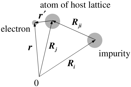
By replacing by (see Fig. 12), becomes
| (85) |
We now assume that acts between the impurity and its nearest-neighbor atoms. We then have , indicating that is independent of . In addition, since is larger than the orbital radius of the 3d electron , is roughly replaced by the dominant component . Namely, we have owing to , . As a result, is approximated as follows:
| (86) |
The distance is here set to be constant independently of ; that is, is written as , where is constant. By substituting eq. (B) with into eq. (B), becomes
| (87) |
where of eq. (B) has been replaced by , i.e., the summation over the nearest-neighbor atoms around the impurity. Next, we consider , which is contained in eq. (B) (in addition, see eq. (B)). This part is expressed as follows:
| (88) |
where is the number of impurities in the volume of . In the calculation process of eq. (B), we have taken the summation about random points on a unit circle in a complex plane and the average over the impurity distributions.[57] In a similar manner, we deal with in eq. (B) to obtain a simple expression. Note, however, that is in fact not contained in this expression and the number of (i.e., ) is also much smaller than . Though this treatment may be crude, we have
| (89) |
where is the number of nearest-neighbor atoms around the impurity.
Using eqs. (B), (B), (B), (B), and (B), we obtain
| (90) | |||
We consider a case in which is much larger than . Equation (B) may then be given by the following approximate expression:
| (92) | |||
| (93) |
with . It is noted that the unit of of eq. (93) is J-1, while that of of eq. (98) is J-1m-3. The unit of in eq. (92) is J2m3, while that of in eq. (97) is J2m6. As to the calculation of and in eqs. (51) - (55), and should be replaced by and , respectively, where is the unit cell volume.
Appendix C s–s Scattering Rate
We derive an expression of the s–s scattering rate of eq. (19).
The scattering rate is originally written as[58, 59]
| (94) |
where and are given by eqs. (77) and (80), respectively. Here, is the wavevector of the incident electron of the spin (i.e., the Fermi wavevector of the spin in the current direction), is the wavevector of the scattered electron of the spin, and is the relative angle between and . In addition, () is the energy of the incident electron (the energy of the scattered electron). Equation (C) is also rewritten as[58]
| (95) |
where is given by
| (96) |
where is a short-range potential due to the impurity, i.e., eq. (81). In the case of the s–s scattering, may be replaced by an approximate potential on the impurity site because such a potential contributes dominantly to . In brief, is approximated as , where is constant. We thus obtain =, which is independent of the spin and the wavevectors. As a result, eq. (C) is expressed as[58, 59]
| (97) | |||
| (98) |
Here, disappears.
Appendix D Matrix Elements
Appendix E Parameters
The resistivity of eq. (17) is first written as
| (102) |
Here, of eq. (19) has been given by
| (103) |
where
| (104) |
with and .[37] The quantity () is the number density[34, 35] (the effective mass[38]) of the electrons in the conduction band of the spin. In addition, is the exchange splitting energy of the conduction electron, where and .
References
- [1] J. Smit: Physica 17 (1951) 612.
- [2] Y. Gondo and Z. Funatogawa: J. Phys. Soc. Jpn 7 (1952) 41.
- [3] I. A. Campbell, A. Fert, and O. Jaoul: J. Phys. C: Metal Phys., Suppl. No.1 (1970) S95.
- [4] R. I. Potter: Phys. Rev. B 10 (1974) 4626.
- [5] T. R. McGuire and R. I. Potter: IEEE Trans. Magn. MAG-11 (1975) 1018.
- [6] J. W. F. Dorleijn: Philips Res. Rep. 31 (1976) 287.
- [7] O. Jaoul, I. A. Campbell, and A. Fert: J. Magn. Magn. Mater. 5 (1977) 23.
- [8] T. R. McGuire, J. A. Aboaf, and E. Klokholm: IEEE Trans. Magn. 20 (1984) 972.
- [9] A. P. Malozemoff: Phys. Rev. B 32 (1985) 6080.
- [10] A. P. Malozemoff: Phys. Rev. B 34 (1986) 1853.
- [11] T. Endo, H. Kubota, and T. Miyazaki: J. Magn. Soc. Jpn. 23 (1999) 1129 [in Japanese].
- [12] M. Ziese: Phys. Rev. B 62 (2000) 1044.
- [13] M. Ziese and H. J. Blythe: J. Phys.: Condens. Matter 12 (2000) 13.
- [14] M. Ziese and S. P. Sena: J. Phys.: Condens. Matter 10 (1998) 2727.
- [15] E. Favre-Nicolin and L. Ranno: J. Magn. Magn. Mater. 272-276 (2004) 1814.
- [16] M. Tsunoda, Y. Komasaki, S. Kokado, S. Isogami, Che-Chin Chen, and M. Takahashi: Appl. Phys. Express 2 (2009) 083001.
- [17] M. Tsunoda, H. Takahashi, S. Kokado, Y. Komasaki, A. Sakuma, and M. Takahashi: Appl. Phys. Express 3 (2010) 113003.
- [18] For example, see L. Berger: J. Appl. Phys. 67 (1990) 5549.
- [19] T. Miyazaki: Spintronics (Spintronics) (Nikkan Kogyo Shimbun, Tokyo, 2007) p. 81 [in Japanese].
- [20] As to eq. (2), see in eq. (48). Also, see ref. \citenTsunoda.
- [21] For a definition of a strong or weak ferromagnet, see, for example, J. F. Janak: Phys. Rev. B 20 (1979) 2206.
- [22] E. Yu. Tsymbal and D. G. Pettifor: Phys. Rev. B 54 (1996) 15314.
- [23] Unpublished data. We evaluated of fcc Ni to be =1.0 10 using a combination of the first principles calculation and the Kubo formula within the semiclassical approximation.[22] The conductivity of the semiclassical approximation corresponded to the Drude formula.[36] Here, we used the tight-binding parameters in ref. \citenpapa.
- [24] For example, see D. A. Papaconstantopoulos: Handbook of the Band Structure of Elemental Solids (Plenum, New York, 1986) p. 95 (bcc Fe) and p. 111 (fcc Ni).
- [25] Unpublished data. We evaluated of Fe4N to be =1.6 10-3 using a combination of the first principles calculation and the Kubo formula within the semiclassical approximation.[22] The conductivity of the semiclassical approximation corresponded to the Drude formula.[36] Here, we used the tight-binding parameters obtained in the previous study.[26]
- [26] S. Kokado, N. Fujima, K. Harigaya, H. Shimizu, and A. Sakuma: Phys. Rev. B 73 (2006) 172410.
- [27] N. F. Mott: Proc. R. Soc. London Ser. A 153 (1936) 699.
- [28] For the resistivity of Fe-Ni and Co-Ni alloys with strongly spin-dependent disorder, see J. Banhart, H. Ebert, and A. Vernes: Phys. Rev. B 56 (1997) 10165.
- [29] For the resistivity of Co-Pd and Co-Pt alloys, see H. Ebert, A. Vernes, and J. Banhart: Phys. Rev. B 54 (1996) 8479.
- [30] A. Fert: J. Phys. C 2 (1969) 1784.
- [31] S. Y. Ren and J. D. Dow: Phys. Rev. B 61 (2000) 6934.
- [32] The resistivity of eq. (7) is obtained from == , =0, and =0, where the suffix of the configuration has been omitted. Here, is the current density, is the velocity of the spin, and is the electric field. As to with =, see refs. \citenCampbell, \citenRen, and \citenFert.
- [33] A. Fert and I. A. Campbell: Phys. Rev. Lett. 21 (1968) 1190.
- [34] H. Ibach and H. Lth: Solid-State Physics: An Introduction to Principles of Materials Science (Springer, New York, 2009) 4th ed., Sect. 9.5. In particular, see eq. (9.58a).
- [35] G. Grosso and G. P. Parravicini: Solid State Physics (Academic Press, New York, 2000) Chap. XI, Sec. 4.1.
- [36] N. W. Ashcroft and N. D. Mermin: Solid State Physics (Thomson Learning, USA, 1976) Chap. 1.
- [37] C. Kittel: Introduction to Solid State Physics (John Wiley & Sons, New York, 1986) 6th ed., Chap. 6.
- [38] For example, see J. Mathon and D. Fraitov: phys. status solidi (b) 9 (1965) 97.
- [39] H. Wang, P.-W. Ma, and C. H. Woo, Phys. Rev. B 82 (2010) 144304.
- [40] S. F. Matar, A. Houari, and M. A. Belkhir: Phys. Rev. B 75 (2007) 245109.
- [41] P. Vargas and N. E. Christensen: Phys. Rev. B 35 (1987) 1993.
- [42] A. Sakuma: J. Phys. Soc. Jpn. 60 (1991) 2007.
- [43] We mention the present tight-binding model. In this model, hybridization of orbitals between different ’s appears only in the presence of the spin–orbit interaction, where is the magnetic quantum number of the d orbital of eq. (75). In other words, we do not consider the matrix elements of the tight-binding Hamiltonian, which give rise to the hybridization between different ’s. Such a matrix element is, for example, an element between and , where = and =. The matrix elements are described in J. C. Slater and G. F. Koster: Phys. Rev. 94 (1954) 1498. On the other hand, the AMR effect is influenced by the orbitals of the specific ’s (see §2.4). Therefore, to quantitatively analyze the AMR effects of real materials, we should take into account the respective realistic band structures. The tight-binding Hamiltonian with the realistic band structure usually includes the matrix elements that lead to the hybridization between different ’s. As a theoretical study based on a realistic band structure, we give ref. \citenPotter.
- [44] I. Galanakis, P. H. Dederichs, and N. Papanikolaou: Phys. Rev. B 66 (2002) 174429.
- [45] J.-H. Park, E. Vescovo, H.-J. Kim, C. Kwon, R. Ramesh, and T. Venkatesan: Nature 392 (1998) 794.
- [46] J. M. De Teresa, A. Barthlmy, A. Fert, J. P. Contour, F. Montaigne, and P. Seneor: Science 286 (1999) 507.
- [47] W. E. Pickett and D. J. Singh: Phys. Rev. B 53 (1996) 1146.
- [48] Y. Miura, K. Nagao, and M. Shirai: Phys. Rev. B 69 (2004) 144413.
- [49] S. Picozzi, C. Ma, Z. Yang, R. Bertacco, M. Cantoni, A. Cattoni, D. Petti, S. Brivio, and F. Ciccacci: Phys. Rev. B 75 (2007) 094418.
- [50] As to La0.64Sr0.36MnO3, see K. Wang, Y. Ma, and K. Betzler: Phys. Rev. B 76 (2007) 144431.
- [51] K. Inomata: Spinelectronics No Kiso To Ouyou (Spinelectronics–Basic and Application) (CMC, Tokyo, 2010) p. 129 [in Japanese].
- [52] D. L. Camphausen, J. M. D. Coey, and B. K. Chakraverty: Phys. Rev. Lett. 29 (1972) 657.
- [53] Z. Zhang and S. Satpathy: Phys. Rev. B 44 (1991) 13319.
- [54] See the literature cited in ref. \citenKittel1. For the resistivity of metals, see Table 3 of p. 144. For the resistivity of semiconductors, see p. 183. For the effective mass divided by the electron mass, see p. 193 and Table 2 of p. 198.
- [55] The resistivity of eq. (44) in this paper corresponds to in ref. \citenZiese, with = or . This correspondence is confirmed from, for example, in eqs. (5) and (6) in ref. \citenZiese, where . Incidentally, using eqs. (22) - (25) in this paper, we obtain and , where has been set. For , also, see eqs. (3) and (4) in ref. \citenMalozemoff2.
- [56] As found from in eqs. (2), (4), (5), and (6) in ref. \citenZiese, in eqs. (2) and (4) might be approximated as , with = or . Here, in eqs. (2) and (4) is usually given by (for example, see in eq. (6) in ref. \citenMalozemoff2).
- [57] G. D. Mahan: Many-Particle Physics (Plenum, New York, 1981) p. 199.
- [58] For example, see Y. Nagaoka, T. Ando, and H. Takayama: KyokuzaiRyoushihourukoukaMitsudoha (Localization, Quantum Hall Effect, and Density Wave) (Iwanami, Tokyo, 1993) p. 24 [in Japanese].
- [59] For example, see J. Inoue and H. Itoh: Spintronics, Kisohen (Spintronics, Basic Edition) (The Magnetics Society of Japan, Tokyo, 2010) Chap 4 [in Japanese].