Exact results for intrinsic electronic transport in graphene
Shijie Hu
Department of Physics, Renmin University of China,
Beijing 100872, China
Institute of Theoretical
Physics, CAS, Beijing 100080, China
Wei Du
Department of Physics, Renmin University of China,
Beijing 100872, China
Guiping Zhang
Department of Physics, Renmin University of China,
Beijing 100872, China
Miao Gao
Department of Physics, Renmin University of China,
Beijing 100872, China
Zhong-Yi Lu
Department of Physics, Renmin University of China,
Beijing 100872, China
Xiaoqun Wang
Department of Physics, Renmin University of China,
Beijing 100872, China
Abstract
We present exact results for the electronic transport properties of
graphene sheets connected to two metallic electrodes. Our results,
obtained by transfer-matrix methods, are valid for all sheet widths
and lengths. In the limit of large width-to-length ratio relevant to
recent experiments, we find a Dirac-point conductivity of
and a sub-Poissonian Fano factor of for
armchair graphene; for the zigzag geometry these are respectively 0 and 1.
Our results reflect essential effects from both the topology of graphene
and the electronic structure of the leads, giving a complete microscopic
understanding of the unique intrinsic transport in graphene.
pacs:
72.80.Vp, 73.22.Pr, 74.25.F-,73.40.Sx
Graphene, a graphite monolayer of carbon atoms forming a honeycomb
lattice, has a distinctive electronic structure whose low energy
excitations are described by massless Dirac fermions. The successful
extraction of micron-scale graphene sheets from a natural graphite
crystal, and their deposition onto an oxidized Si wafer exp0 ,
was a truly seminal event which ushered in a new era of realistic
experimental and theoretical exploration. The subsequent explosion
of graphene activity has focused on fundamental questions concerning
the transport properties of relativistic particles in graphene and on
its potential applications as a high-mobility semiconductor.
Theoretical predictions fermion for two-dimensional Dirac-fermion
systems give an intrinsic conductivity of order . Minimal
conductivities around this value were observed at the Dirac point exp1
in Ref. exp0 , while later measurements exp3 suggested that
when the width-to-length ratio of the
sample is sufficiently large. This is the value obtained using massless
Dirac fermions and graphite leads in a Landauer-Büttiker (LB) formulation
Landauer1 ; Landauer2 . It is associated with a maximum of 1/3 in the
Fano factor, Landauer2 , which reflects the partial transmission
of quantized charge through the finite graphene system. Measurements of the
current shot noise in both ballistic fano1 and diffusive fano2
graphene systems have indeed found that in short and wide
samples. Many authors have addressed different aspects of the graphene
transport problem, which we summarize below. While the finite conductivity
and suppressed Fano factor are generally expected in graphene systems, the
underlying physics remains rather poorly understood, not least because the
carrier density at the Dirac point is zero.
In this paper, we consider graphene sheets of both armchair (AGS) and
zigzag (ZGS) geometry, connected to two metallic leads as illustrated
in Fig. 1. By establishing a transfer-matrix formulation within
this minimal model, we present exact results for the anomalous intrinsic
transport properties of graphene. We demonstrate that the AGS and ZGS are
completely different, and explain in detail the non-universal dependence
of and on geometry, filling, and gate voltage.
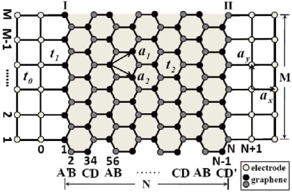
Figure 1: Schematic representation of an armchair graphene
sheet connected to electrodes at interfaces I and II. Primitive vectors
and for the electrodes and and
for the sheet give length and
width ; with Å for
graphene. The ZGS case, obtained by a rotation, has length and width , still with
sites.
The low-energy properties of graphene can be described by a nearest-neighbor,
one-orbital tight-binding model for -electrons on a hexagonal lattice,
(1)
where is an electron creation operator at lattice
site , denotes
nearest-neighbor sites, is the hopping integral, and the
chemical potential. The two electrodes are represented by semi-infinite
rectangular strips with hopping , while the interface hopping is
. We take the interface contact to be perfect and impose open boundary
conditions on the two free edges of the sheet; it is the geometry of these
edges which determines our nomenclature (AGS or ZGS). Because graphene has
two sublattices, sheets of size lattice sites are taken to have
width and length (AGS) or (ZGS) with an integer.
We begin with the AGS case (Fig. 1) by constructing a
transfer-matrix equation for the scattering of electrons between two
electrodes. In the Schrödinger equation , the wave function is represented as [ for ],
with the complex coefficients
to be determined. is the Fermi energy of the
electrodes, which is set by their occupation . There are
right- and left-traveling waves (channels) in each electrode,
each channel characterized by a transverse wavenumber with . The longitudinal
wavenumber is related to by .
With a unit-amplitude, right-traveling wave incident on the sheet in
the th channel of the left electrode,
(2)
for the left and right electrodes, where and
are respectively reflection and transmission
coefficients from channel to . For each site
in the sheet, , where specify the
nearest-neighbor sites of and . We express the coefficients for a given
as the vector in order to connect with its
neighboring slices through the transfer matrix
,
(7)
A translation period involves
four different slices (Fig. 1), so
cycles through the four block matrices
(12)
(17)
where is lower-bidiagonal with nonzero elements equal to 1,
is the inverse of , and is the identity.
Recursive application of Eq. (7) for slices ( translation
periods) relates the coefficients and at the left
and right interfaces through
where .
By considering the one-period transfer matrix ,
one finds that the transverse modes in the AGS are unmixed by
scattering processes, remaining independent and retaining the
free-particle dispersion . This
makes the LB formalism underlying our transport calculations
particularly appropriate. Thus Eq. (Exact results for intrinsic electronic transport in graphene) can be decomposed
into the set of binary linear equations
These expressions are completely general within the LB framework, and
are applicable for all sheet sizes .
For the purposes of this Letter, we focus on the physical insight
contained in Eq. (19) for the situation relevant to most
graphene experiments, namely wide electrodes patterned onto the
sample with rather narrow separation fano1 ; fano2 . In this
limit of large , the sum in Eq. (19) is
replaced by an integral over . For convenience we set , which creates no special symmetries. The Dirac-point
conductivity and the corresponding Fano factor may
then be expressed analytically as
(20)
where is the Dirac-point wavenumber of the AGS and
is determined by . At half-filling of the electrodes,
i.e. and , we obtain and .
Our results for the AGS are similar but not identical to the values
and of Ref. Landauer2 . While the electronic
structure of the electrodes leads to a small quantitative difference
between the two studies, we will show below that the symmetry-breaking
effect of the electrode interfaces causes a strong qualitative difference.
The fact that at the Dirac point , despite
the vanishing density of states, is an intrinsic property of the AGS quite
distinct from conventional mesoscopic systems.
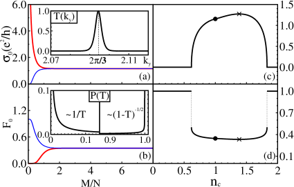
To analyze the physical origin of this behavior, Fig. 2
shows the full dependence of and on and on
the aspect ratio of the sheet for . In Figs. 2(a)
and (b), for , and alternate as increases
between semiconducting and metallic behavior, the latter obtained
when mod and there exists a
resonant channel with at [inset Fig. 2(a)].
As the sheet width is increased, the two branches merge at with and independent of ; only when are sufficiently many channels with
available that their contributions to the sum in Eq. (19)
are constant. For such sheets [inset Fig. 2(b)], channels with contribute to with a distribution while channels with have prob . Although resembles the universal
bimodal distribution for a disordered mesoscopic system, which also
has , the underlying physics is completely different:
the sub-Poissonian behavior is caused by the interference of
relativistic quantum particles, which results in transport
contributions away from the
resonant channel [inset Fig. 2(a)]. This type of behavior, namely
and , is obtained in the AGS only
for [Figs. 2(c) and (d)].
Figure 2: (Color online) Dirac-point conductivity
(a,c) and Fano factor (b,d) as functions of for (a,b)
and of with (c,d). Dots denote
in (c) and in (d) at , while crosses
denote in (c) and in (d), obtained at
. Insets: transmission probability around
in (a) and its distribution (see text) in (b).
Calculations performed with in the system of Fig. 1.
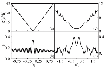
Figure 3 shows the effects of a gate voltage on and for
. For a finite sheet, the number of Fermi momenta (number
of energy bands intersected) increases with , each peak in
and corresponding to one more contributing resonant
channel. When the sheet is sufficiently wide [Fig. 3(a)], channels
are added at nearly equal intervals, resulting in almost periodic
oscillations, whereas for [Fig. 3(b)] the effects
of added channels appear quasi-periodic. Superposed on the
oscillation is a linear and slightly asymmetric behavior of
about the Dirac point. The former is a consequence of the linear
dispersion of graphene and the latter of the electron-hole asymmetry
caused by the electrodes Beenakker . Thus our exact results
illustrate the inherent dependence of experimental observations on
both and exp1 ; exp3 , and demonstrate further that
such behavior can be intrinsic, rather than appearing only as a
consequence of sample disorder or interfacial defects.
Figure 3: Conductivity (a,c) and Fano factor (b,d) for the AGS
with and , shown as functions of for
(a,b) and (c,d).
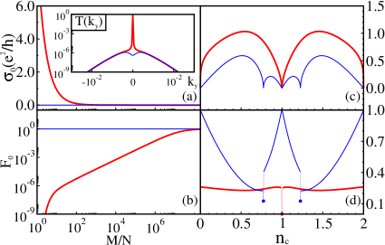
We turn now to the ZGS. The geometry of this case requires a
transfer matrix expressed in terms of two 22
block matrices and a quartic form of Eq. (Exact results for intrinsic electronic transport in graphene) for ,
which is solved numerically to obtain and from
Eq. (19). Figure 4 shows the dependence of and
on , again with and . The
ZGS also possesses metallic and semiconducting branches, which
alternate with respect to the sheet length rather than to its
width . The asymptotic behavior is metallic, with for mod, and
semiconducting with otherwise
[Fig. 4(a)]. The corresponding Fano factors [Fig. 4(b)] are and , the two branches merging only when . Graphene sheets in this limit of would therefore
have and at the Dirac point, implying a
Poissonian shot-noise quite different from the AGS. A finite minimal
conductivity, (reaching its
maximal value when ), and a sub-Poissonian are
obtained for all [Figs. 4(c) and (d)].
The origin of the contrasting intrinsic transport properties of the
AGS and ZGS for the Dirac point lies in the special nature of zigzag
chains in graphene. The key point is how this affects scattering at
the interfaces. Because for any site in the sheet, the wavenumber of extended
states is when projected onto the zigzag chain direction, and
zero in the orthogonal direction. In the AGS, zigzag chains are parallel
to the interfaces so that for mod. Thus
the incident traveling wave is not deformed at the interface and there
is no interfacial scattering. Consequently, and in a regime of width about [inset Fig. 2(a)],
resulting in a finite after the summation in Eq. (19)
if [Fig. 2(c)]. In the ZGS, zigzag chains
connect the left and right electrodes, , and the armchair
interfaces involve two sublattices, with two values of
corresponding to each . This induces interfacial scattering.
As a consequence, for the transmission amplitudes are
suppressed very strongly for any and [inset Fig. 4(a)], where is a very small background
of width arising from interfacial scattering. Neither term
contributes to the integral in the limit of large and , whence
and . When details , imaginary
values appear for some channels , giving contributions
to over a greater width and leading to a finite
[Fig. 4(c)]. Thus it is the topological difference in the geometry
along and across a hexagonal lattice which results in two fundamentally
different types of interfacial scattering, and hence in the contrasting
intrinsic transport properties of AGS and ZGS systems. This microscopic
insight was not included in any previous studies.
Figure 4: (Color online) (a,c) and (b,d) for a ZGS, shown as
functions of at (a,b) and of for (c,d).
Inset: around . Red and blue curves indicate respectively
metallic and semiconducting situations, calculated with and 999.
Many investigations of graphene transport may be found in recent
literature. Augmenting the general results cited above, experimental
studies of the conductivity minimum have addressed the coherence of
Dirac-point transport rhea , the role of contacts and sample
edges rlea , and how interface charging leads to asymmetric
gate-voltage effects rhea2 . Many theoretical studies have
considered transmission coefficients in a finite graphene system,
all restricted (as here) to the case of non-interacting electrons:
from its weak interactions and the vanishing density of states at
the Dirac point, the fundamental transport properties of graphene
are expected to emerge at the band-structure level. These
investigations all differ from ours in the approximations applied,
or in system size and geometry, or in the method of calculation, and
hence in the nature of their conclusions. In an effective contact
model rs for a sufficiently large system, mode selection at
the Dirac point makes all leads equivalent. Numerical treatments, of
the same model rrs and in a more general framework
rblvkc , have probed size, gate-voltage, and impurity effects.
While these and other studies Landauer2 ; rbm note that the AGS
and ZGS cases should differ, the fundamentally different nature
(, ) of the ZGS case and the microscopic
origin of the different intrinsic transport properties have been
missed. Further, because we have analyzed the intrinsic transport
arising due to lead and interface geometry, we may conclude that
disorder effects are not required to obtain the anomalous behavior
observed in experiment exp1 ; exp3 ; rhea .
To conclude, we have presented exact solutions of the
transfer-matrix equations for graphene sheets with metallic
electrodes. Our results are microscopic and completely general, and
can be used to show that the Dirac-point conductivity and the Fano
factor tend respectively to and for armchair graphene
sheets in the short and wide limit relevant to experiments. The same
quantities tend to 0 and 1 respectively for zigzag graphene sheets.
Our exact results suggest that the measured finite minimum
conductivity and sub-Poissonian Fano factor are the consequence of
armchair rather than zigzag graphene systems, and show how this
fundamental difference depends on the availability of resonant
transmission channels, which is determined in turn by the geometry
of the hexagonal lattice.
The authors thank B. Normand, E. Tosatti, B. G. Wang, X. R. Wang, X. C.
Xie, Lu Yu, and Y. S. Zheng for fruitful discussions. This work was
supported by the Chinese Natural Science Foundation, Ministry of Education,
and National Program for Basic Research (MST).
References
(1) K. S. Novoselov et al., Science 306, 666 (2004).
(2) E. Fradkin, Phys. Rev. B 33, 3263 (1986);
N. H. Shon and T. Ando, J. Phys. Soc. Japan 67, 2421 (1998);
E. V. Gorbar, V. P. Gusynin, V. A. Miransky, and I. A. Shovkovy,
Phys. Rev. B 66, 045108 (2002).
(3) K. S. Novoselov et al., Nature 438, 197 (2005).
(4) F. Miao et al., Science 317, 1530 (2007).
(5) M. I. Katsnelon, Euro. Phys. J. B 51, 157 (2006).
(6) J. Tworzydlo et al., Phys. Rev. Lett. 96,
246802 (2006).
(7) R. Danneau et al., Phys. Rev. Lett. 100,
196802 (2008).
(8) L. DiCarlo, et al., Phys. Rev. Lett. 100,
056801 (2008).
(9) The distribution of the transmission probability is defined as
.
(10) When graphite leads are used, is symmetric
Landauer2 .
(11) H. B. Heersche et al., Nature 446, 56 (2007).
(12) E. J. H. Lee et al., Nature Nanotech. 3,
486 (2008).
(13) B. Huard, N. Stander, J. A. Sulpizio, and D. Goldhaber-Gordon,
Phys. Rev. B 78, 121402 (2008).
(14) H. Schomerus, Phys. Rev. B 76, 045433 (2007).
(15) J. P. Robinson and H. Schomerus, Phys. Rev. B 76, 115430
(2007).
(16) S. Barraza-Lopez, M. Vanević, M. Kindermann, and M. Y.
Chou, Phys. Rev. Lett. 104, 076807 (2010).
(17) Y. M. Blanter and I. Martin, Phys. Rev. B 76, 155433
(2007).
(18) Detailed analysis for will be presented
elsewhere.