Interface tension of the 3d 4-state Potts model using the Wang-Landau algorithm

Abstract:

We study the interface tension of the 4-state Potts model in three dimensions using the Wang-Landau algorithm. The interface tension is given by the ratio of the partition function with a twisted boundary condition in one direction and periodic boundary conditions in all other directions over the partition function with periodic boundary conditions in all directions. With the Wang-Landau algorithm we can explicitly calculate both partition functions and obtain the result for all temperatures. We find solid numerical evidence for perfect wetting. Our algorithm is tested by calculating thermodynamic quantities at the phase transition point.

Preprint: CP3-Origins-2011-038 and DIAS-2011-31

1 Introduction

The interface free energy on a $D$-dimensional lattice, with size $L_{1}\times L_{2}\times\dots\times L_{D}\equiv L_{1}\times V_{D-1}$, is obtained from the ratio of two partition functions

$$F_{s}=-\log\frac{Z_{a}}{Z_{p}}-\log L_{1},$$ (1)

where $Z_{p}$ is a partition function with periodic boundary conditions and $Z_{a}$ has periodic boundary conditions in $D-1$ directions and a twisted boundary condition, which develop a topological excitation, in the direction labelled by 1. In other words, the topological excitation forced by the twisted boundary condition induces an interface in to the system, and the free energy of the interface is obtained by subtracting the free energy of the bulk ($-\log Z_{p}$) out of it. The $\log L_{1}$ term has been subtracted since the interface can form at any of the $L_{1}$ points. The interface tension is then

$$\sigma=\lim_{L_{i}\rightarrow\infty}\frac{F_{s}}{V_{D-1}}.$$ (2)

The difficulty in calculating the interface tension arises from the fact that the partition functions are hard to calculate using traditional simulation methods, since they have exponential fluctuations in volume [1, 2]. Therefore, the standard approach has been to relate the interface tension to quantities that are easier to determine with Monte Carlo simulations [3]. However, these methods generate large systematic and/or statistical errors.

In [4] we have proposed a new method to calculate interface tensions. It is based on the Wang-Landau [5] algorithm. This algorithm enables us to calculate numerically the density of states of the system, and from this the partition function can be obtained as a numerical integral. As a test system we used the 3d 4-state Potts model. We were also able to provide solid numerical evidence for perfect wetting.

2 Wang-Landau algorithm

Consider a system with partition function

$$Z=\sum_{\{i\}}\exp(-\beta E_{i})\equiv\sum_{i}g(E_{i})\exp(-\beta E_{i}).$$ (3)

where $\{i\}$ is a generic configuration and $g(E_{i})$ the density of states with energy $E_{i}$. The Wang-Landau algorithm [5] estimates directly the density of states $g(E_{i})$. The algorithm is based on a simple observation: If the state of a system is changed randomly, and the probability to visit a given energy level $E$ is $1/g(E)$, a random walk in $E$ generates a flat distribution across the energy levels.

The algorithm consists of following steps

• Start with any lattice configuration and a nonzero density of states $g(E)$.

• Change a random site to a random value.

• Accept the change with a probability

  $$P=\min\left\{\frac{g(E_{\rm old})}{g(E_{\rm new})},1\right\}$$ (4)

  and if the change is rejected set $E_{\rm new}=E_{\rm old}$.

• Update $g(E_{\rm new})$ and a histogram $H(E_{\rm new})$

  $$g(E_{\rm new}) \rightarrow fg(E_{\rm new})\ ,$$

  $$H(E_{\rm new}) \rightarrow H(E_{\rm new})+1\ .$$ (5)

• Set $E_{\rm old}=E_{\rm new}$ and repeat from 2 until $g(E)$ has converged. Then reduce $f\rightarrow\sqrt{f}$ and set $H(E)$ to zero.

• Repeat from 2 until $f$ reaches some small enough value.

The algorithm satisfies detailed balance only in the limit $f\rightarrow 1$. In more detail, the transition probabilities satisfy

$$\frac{1}{g(E)}p(E\rightarrow E^{\prime})=\left\{\begin{array}[]{lcl}\frac{1}{fg(E^{\prime})}p(E^{\prime}\rightarrow E),&{\rm if}&g(E)\geq fg(E^{\prime})\\ \frac{1}{g(E)}p(E^{\prime}\rightarrow E),&{\rm if}&g(E^{\prime})<g(E)<fg(E^{\prime})\\ \frac{1}{g(E^{\prime})}p(E^{\prime}\rightarrow E),&{\rm if}&g(E)<g(E^{\prime})\end{array}\right..$$ (6)

At $f=1$ we obtain the detailed balance condition

$$\frac{1}{g(E)}p(E\rightarrow E^{\prime})=\frac{1}{g(E^{\prime})}p(E^{\prime}\rightarrow E).$$ (7)

Hence, with $f\neq 1$ the algorithm produces a $g(E)$ that favors the large values over the small ones. However, in practice this does not seem to generate problems as long as the number of iterations is large enough, s.t., the statistical errors are larger than the systematic ones.

As a convergence criterion we follow [6], and require that each energy level is visited $1/\sqrt{\ln f}$ times since after this statistical errors are not expected to decrease. This criterion might suffer from systematic errors, which can lead the system to convergence to a wrong density of states [7, 8]. A safer criterion would be to require $1/\ln f$ visits to each energy level. However, for the level of accuracy requested in our simulations, the results obtained with these two criteria are identical within the statistical errors. See next section.

3 Algorithm testing

As a test case we use 4-states Potts model in 3d. The Hamiltonian of the model is

$$H=2J\sum_{\langle ij\rangle}\left(\frac{1}{4}-\delta_{q_{i},q_{j}}\right),$$ (8)

where $J$ is the strength of the interaction, $q_{i}\in[0,3]$, $\delta_{q_{i},q_{j}}$ is the Kronecker delta function of the spin variables $q_{i},q_{j}$ on neighbor sites $i,j$ and the sum $\langle ij\rangle$ is over nearest neighbors.

To obtain statistical error estimates for measured quantities we perform 20 separate runs with twisted and untwisted boundary conditions. For each run we do 23 iterations, meaning that $f_{\rm min}\approx 1+1.3\times 10^{-7}$ during the last step (we start by setting $f=3$). The simulations are done on lattice sizes $L=16,20,24,28,32,40,48$, and $56$.

Figure 1: Specific heat calculated using three different convergence requirements: flat histogram (left), $1/\ln(f)$ visits required (middle) and $1/\sqrt{\ln f}$ visits required (right). The solid line is the result of the middle panel after 27 iterations.

Figure 2: Left: Normalized difference between the specific heat obtained with two different convergence criteria. The label $a$ indicates the criterion requiring $1/\sqrt{\ln f}$ visits at iteration 23 and $b$ $1/\log f$ visits at iteration 27 . Right: Transition temperature calculated with three different methods.

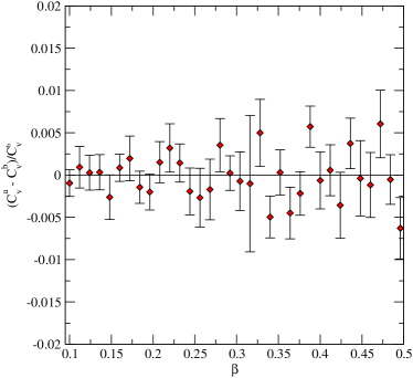
To test the convergence criteria and the systematic errors arising from the update, we measure the specific heat

$$C=\frac{\beta^{2}}{L^{3}}\left(\langle E^{2}\rangle-\langle E\rangle^{2}\right).$$ (9)

We have used three different convergence criteria. The first requires flat histogram, the second $1/\ln(f)$ visits and third $1/\sqrt{\ln(f)}$ visits to each energy level. In Fig. 1 we have plotted the specific heat calculated with the different convergence criteria as a function of the number of iterations. At about iteration 20 all the three criteria provide convergence to the same value. In the left panel of Fig. 2, we have plotted the normalized difference of the specific heat obtained with the third criterion at iteration 23 and the specific heat obtained with the second criterion at iteration 27. The differences are completely dominated by statistical errors, and hence we do not expect to have systematic errors due to the finite $f$ or wrong convergence of $g(E)$.

$\beta^{1}_{c}$	0.3143104(9)
$\beta^{2}_{c}$	0.3143103(9)
$\beta^{3}_{c}$	0.3143102(9)
$\beta_{c}$	0.3143103(9)
$\beta_{\rm MM}$	0.3143103(5)
$\beta_{\rm BBD}$	0.3143041(17)

$\Delta e$	1.16454(16)
$\Delta e_{\rm MM}$	1.16492(12)
$\Delta e_{\rm BBD}$	1.16294(61)

Table 1: Comparison of our results with previous studies for the transition temperature (left) and the latent heat (right). The result with label MM are from [10] and BBD from [9].

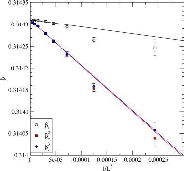
To additionally test our algorithm we compute the critical temperature and latent heat and compare them with the results of [9] and [10]. Following [9], we use three different definitions for the critical $\beta$ at finite volume. The first, $\beta_{c}^{1}$, is defined to be the value for which the canonical distribution $P(E,\beta)=g(E)e^{-\beta E}$ has two equal maxima, the second, $\beta_{c}^{2}$, is the position of the central energy of the latent heat, and the third, $\beta_{c}^{3}$, is the position of the maximum of the specific heat Eq. (9). After extrapolating to infinite volume these definitions agree with each other. See Fig. 2, right.

The latent heat $\Delta e$ can be obtained from the maxima of specific heat

$$C_{\rm max}(L)=c+\frac{1}{4}(\beta_{c})^{2}(\Delta e)^{2}L^{3}.$$ (10)

Our results and those of [9, 10] are collected in Table 1. The discrepancy with [10] is less than two standard deviations for all the quantities. The agreement is not as good with [9], but in this work smaller lattices are used.

4 Interface tension

Figure 3: Left: The order-order interface tension as a function of $\beta$. Right: The probability distribution at the critical temperature. The maxima are normalized to one.

We consider two different kinds of interface. The first, order-order interface, is between two regions of space that are in two different ordered vacua. Near the critical temperature, the interface tension assumes the form (see [11, 12])

$$\sigma_{\rm oo}(L)=\sigma_{\rm oo}+\frac{c_{2}}{L^{2}}+\frac{c_{4}}{L^{4}}\dots,$$

from which the asymptotic behavior can be extracted. In our simulations we have truncated the series to $\mathcal{O}(L^{-4})$, since the corrections from higher order terms are same the size of the statistical errors. For the fit we use only the points for which

$$L\sqrt{\sigma_{\rm oo}}\geq 6$$

$$\frac{1}{\sqrt{\sigma_{\rm oo}}}\geq 3.$$ (11)

The former condition is to reduce finite size effects and the latter one is dictated by the fact that Eq. (4) is only expected to hold at large distances.

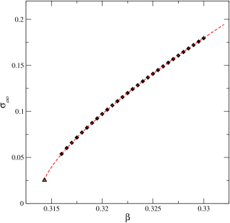
Near $\beta_{c}$, the behavior of $\sigma_{\rm oo}$ can be parametrized as

$$\sigma_{\rm oo}(\beta)=\sigma_{\rm oo}(\beta_{c})+a(\beta-\beta_{c})^{\rho}.$$ (12)

This functional form represents the data well. A fit with 9 degrees of freedom has $\chi^{2}/9=0.11$. The values are $\sigma_{oo}=0.0249(6)$ and $\rho=0.76(4)$. See the right panel of Fig. 3.

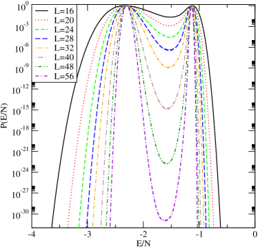
The other interface, the order-disorder interface, is an interface that separates an ordered state from the disordered state. It is defined only at the critical temperature for systems with a first order phase transition. The order-disorder interface can be calculated from the probability distribution. Namely, if $P_{\rm max}$ is the peak of the histogram when the two maxima have equal height, and $P_{\rm min}$ is the minimum between the peaks, the tension is given by (see [13, 14])

$$2\sigma_{\rm od}=\frac{1}{L^{2}}\log\left(\frac{P_{\rm max}}{P_{\rm min}}\right)\ .$$ (13)

Our data for $P$ are displayed in the right pane of Fig. 3.

To obtain the asymptotic form we use a fitting function of the form.

$$2\sigma_{\rm od}=\frac{\log L}{L^{2}}-2\sigma_{\rm od}+\frac{c_{2}}{L^{2}}+\frac{c_{4}}{L^{4}}.$$ (14)

A fit of the date according to Eq. (14) yields $2\sigma_{do}=0.0252(4)$. The insertion of a term $c_{3}/L^{3}$ in the fitting function, justified by the use of the estimator (13), gives a compatible result.

Figure 4: Illustration of wetting (left) and perfect wetting (right). In the case of perfect wetting the order-order interface is twice the order-disorder interface.

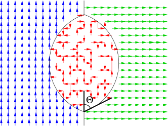
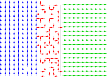
The ratio of order-order to disorder-order interface tensions gives the wetting angle

$$\frac{\sigma_{\rm oo}}{2\sigma_{\rm od}}=\cos\theta,$$ (15)

where for perfect wetting $\theta=0$. See Fig. 4. Our result is a clear indication that perfect wetting holds for the three dimensional Potts model. This result has also been conjectured for the two-dimensional Potts model [15].