Maintaining Quantum Coherence in the Presence of Noise by State Monitoring

Abstract

Unsharp POVM measurements allow the estimation and tracking of quantum wavefunctions in real-time with minimal disruption of the dynamics. Here we demonstrate that high fidelity state monitoring, and hence quantum control, is possible even in the presence of classical dephasing and amplitude noise, by simulating such measurements on a two-level system undergoing Rabi oscillations. Finite estimation fidelity is found to persist indefinitely long after the decoherence times set by the noise fields in the absence of measurement.

Maintaining high-fidelity quantum control is a central requirement in a variety of technologies ranging from nuclear magnetic resonance to quantum based precision measurement Chou et al. (2010). Quantum control is usually restricted to a finite time window as a result of the unavoidable influence of decohering environments, and the control lifetime is often extended through the use of decoherence free subspaces Palma et al. (1996), or dynamical decoupling Cywinski et al. (2008).

In this communication we discuss a scheme which relies on a sequence of consecutive POVM (Positive Operator-Valued Measure) measurements to maintain quantum control. We demonstrate that the time-evolution of a driven, isolated two-level quantum system, subject to classical dephasing and amplitude noise, can be monitored long beyond its Rabi coherence time. In fact, the wavefunction can in principle be tracked indefinitely with finite fidelity, unlike systems controlled by dynamical decoupling that ultimately undergo complete loss of coherence. The control scheme relies on periodic application of special POVM measurements said to be “unsharp” Busch et al. (1995). Such measurements have previously been shown to allow faithful monitoring of Rabi oscillations if the general form of a time-independent Hamiltonian is known Audretsch et al. (2001, 2007) and no external noise is present.

A scheme for updating a state estimate during continuous measurements Belavkin V.P. (1989) - the continuum limit of the technique employed here - has been presented in Diosi et al. (2006). In that scheme the state evolution of the system, its estimated state, and the measurement readout is described by three coupled stochastic differential equations, which indicate that the state estimate converges to the real state for a broad class of systems, cf. Konrad et al. (2010). Continuous measurements have also been shown to drive statistical mixtures of spatial wavepackets into pure states, which can be entirely determined by the measurement record alone Doherty et al. (1999).

Specific experimental implementations of unsharp measurements have been suggested in the context of Bose-Einstein Condensates Corney and Milburn (1998), cavity QED Audretsch et al. (2002a) and coupled quantum dots Korotkov (2003); Oxtoby et al. (2008). Several realizations of the related topic of “weak-value” measurement have been demonstrated through measurements of photon momentum Ritchie et al. (1991); Dixon et al. (2009); Hosten and Kwiat (2008); Koksis et al. (2011). In addition, experiments of “continuous weak measurement” were implemented using a cold cesium vapor Silberfarb et al. (2005). These realizations all employed ensemble measurements, while we here show monitoring of a single, isolated quantum system by repeated measurement, as the system evolves.

We consider a two-level system undergoing Rabi-oscillations. In a frame rotating at the two-level transition frequency it evolves under the Hamiltonian

$$H_{R}=\hbar\frac{\Omega_{R}}{2}\hat{\sigma}_{x},$$ (1)

where $\hat{\sigma}_{x}$ is the Pauli matrix which generates rotations about the $x$-axis and $\Omega_{R}$ the Rabi frequency, which is assumed to be known. At the same time we assume the system is under the influence of random classical noise fields $\beta(t)$ and $\alpha(t)$, causing dephasing and amplitude fluctuations, respectively, through a noise Hamiltonian

$$H_{N}=\hbar\beta(t)\hat{\sigma}_{z}+\hbar\alpha(t)\hat{\sigma}_{x}.$$ (2)

Each noise field is characterized by a power spectrum which is related to its autocorrelation function

$$C^{(2)}(\tau)=\frac{1}{T}\int_{0}^{T}\xi(t)\xi(t+\tau)dt$$ (3)

through

$$P_{\xi}(\omega)=\int C^{(2)}(\tau)e^{i\omega\tau}d\tau$$ (4)

where $\xi(t)=\alpha(t),\beta(t)$.

The estimation strategy rests on carrying out POVM measurements periodically Nielsen M.A. and Chuang (2002), and updating the state estimate based on the measurement outcomes. Quite generally, a POVM measurement with outcome $n$, which was carried out on a system in the state $|\psi\rangle$, will result in a state after the measurement given by

$$|\psi_{n}\rangle=\frac{\hat{M}_{n}|\psi\rangle}{\sqrt{p(n|\psi)}}.$$ (5)

Here $\hat{M}_{n}$ is the so-called “Kraus operator” corresponding to the measurement outcome $n$, and

$$p(n|\psi)=\langle\psi|\hat{M}^{\dagger}_{n}\hat{M}_{n}|\psi\rangle$$ (6)

is the probability to detect outcome $n$, conditioned on the system being in state $|\psi\rangle$.

In an estimation experiment a sequence of periodic measurements, with period $\tau$, are applied to the system as it evolves in time Audretsch et al. (2001). Despite the dynamics, the state change due to the measurement can still be described by Eq. (5) if each measurement is executed much faster than all other dynamical timescales (impulsive measurement approximation). In between measurements the time evolution is described by the operator

$$\hat{U}_{j}=\mathcal{T}\left[\exp{(-\frac{i}{\hbar}\int_{t_{j}}^{t_{j}+\tau}(H_{R}+H_{N}(t))dt)}\right],$$ (7)

where $\mathcal{T}$ is the time-ordering operator. At $t=N\tau$, after $N$ measurements, the system is, up to the appropriate normalization constant, in the state

$$|\psi(N\tau)\rangle=\hat{M}_{n_{N}}\hat{U}_{N}\hat{M}_{n_{N-1}}\hat{U}_{N-1}...\hat{M}_{n_{1}}\hat{U}_{1}|\psi\rangle.$$ (8)

To estimate the state of the system the same sequence of operators corresponding to the measured outcomes in Eq. (8) are applied to an initial guess $|\psi_{e}\rangle$ (cp. Diosi et al. (2006)), but
(1) the initial estimate of the state $|\psi_{e}\rangle$ can be taken as an arbitrary state vector on the Bloch sphere and
(2) in between measurements the state estimate is assumed to evolve only through the Hamiltonian Eq. (1), since the experimenter does not know what the instantaneous values of the noise fields are. As we’ll see in what follows it is still possible to estimate the state of the system without detailed knowledge of the noise fields. Our approach differs from Audretsch et al. (2007) where the Rabi frequency was assumed to be unknown and one of the aims was to determine its value through a Bayesian estimator in the absence of noise.

We now define two projectors $\hat{P}_{+}=\frac{1}{2}(\mathbb{1}+\hat{\mathbf{r}}\cdot\hat{\sigma})$ and $\hat{P}_{-}=\frac{1}{2}(\mathbb{1}-\hat{\mathbf{r}}\cdot\hat{\sigma})$, where $\mathbb{1}$ is the identity operator, $\hat{\mathbf{r}}=(\delta,\zeta,\chi)$ a unit vector on the Bloch sphere, and $\hat{\sigma}=(\hat{\sigma}_{x},\hat{\sigma}_{y},\hat{\sigma}_{z})$. In terms of these it is possible to construct POVM measurement operators $\hat{M}_{0}=\sqrt{p_{0}}\;\hat{P}_{+}+\sqrt{1-p_{0}}\;\hat{P}_{-}$, and $\hat{M}_{1}=\sqrt{1-p_{0}}\;\hat{P}_{+}+\sqrt{p_{0}}\;\hat{P}_{-}$, related via $M_{0}^{\dagger}M_{0}+M_{1}^{\dagger}M_{1}=\mathbb{1}$, and $0\leq p_{0}\leq 0.5$. The strength of a single measurement is quantified by $\Delta p=(1-p_{0})-p_{0}=1-2p_{0}$ Audretsch et al. (2002b). However, the strength of a sequence of measurements depends also on the period $\tau$ between two consecutive measurements. For fixed $\Delta p$ a shorter (longer) period $\tau$ means a stronger (weaker) influence of the sequential measurement. The strength of the state disturbance due to this sequential measurement is best quantified by the rate $\gamma_{m}=1/\tau_{m}$ with $\tau_{m}=2\tau/(\Delta p)^{2}$ Audretsch et al. (2002b). The strength $\gamma_{m}$ is the expected rate at which an arbitrary initial state is reduced to an eigenstate of the measured observable, in the absence of dynamics other than measurement Audretsch et al. (2001).

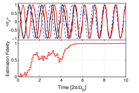
Figure 1: Wavefunction estimation in the absence of noise for a specific realization of $\alpha(t)$ and $\beta(t)$ (single run). (a) Expectation value $\langle\hat{\sigma}_{z}\rangle$ for blackline - true expectation value, red line - estimated expectation value, dashed blue line - expectation value in the absence of measurements, (b) Estimation fidelity.

To set the stage we illustrate the method in the absence of noise, i.e. $\beta(t)=\alpha(t)=0$. We simulate an experiment in which we choose $\Delta p=0.2$ and $\hat{\mathbf{r}}=(0,0,1)$ which corresponds to an unsharp measurement of $\hat{\sigma}_{z}$ (cp. Audretsch et al. (2007)). We carry out a measurement every $\tau=T_{R}/10$, where $T_{R}=2\pi/\Omega_{R}$ is the Rabi-period. The resulting measurement strength is thus smaller than the Rabi-frequency ($\gamma_{m}=\Omega_{R}/10\pi$), which is required in order not to disturb the oscillations too strongly. For a measurement strength $\gamma_{m}$ much greater than $\Omega_{R}$ the state would be projected onto an eigenstate of the observable $\hat{\sigma}_{z}$ before a single oscillation can take place, and the dynamics would freeze (similarly to the Quantum Zeno Effect Misra and Sudarshan (1977)). The result of each measurement is chosen at random, commensurately with the probabilities prescribed by Eq. (6). The initial state estimate is chosen orthogonal to the initial state vector, a limiting case for which the estimation procedure might be expected to have some difficulty.

In Fig. 1(a) we plot the expectation value of $\langle\hat{\sigma}_{z}\rangle$ for the true state (black line) and the state estimate (red line) for one single run of the measurement experiment (i.e. one specific realization of $\alpha(t)$ and $\beta(t)$). The state (black line) undergoes Rabi oscillations, but with measurement induced random phase shifts as compared to the undisturbed oscillations (dashed blue line). The oscillations including the influence of the measurement are monitored accurately by the estimate (red line) after about 6 Rabi periods. After this time not only the expectation value of the measured observable $\hat{\sigma}_{z}$ with respect to the true and estimated state, but also the states themselves coincide as is indicated by the plot of the estimation fidelity $F(t)=|\langle\psi_{est}|\psi\rangle|^{2}$ in Fig. 1(b). Asymptotically the fidelity tends to unity, indicating the perfect state monitoring of a single system, in real time, in the absence of noise.

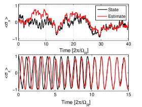
Figure 2: State estimation in the presence of dephasing and amplitude noise. (a) Expectation value of $\hat{\sigma}_{x}$ and (b) expectation value of $\hat{\sigma}_{z}$ for a specific realization of $\alpha(t)$ and $\beta(t)$. Here we used $\Delta\beta=0.05,\Delta\alpha=0.005$, $\Delta p=0.2$, and $\hat{\mathbf{r}}=(0.43,0,0.9)$. Note (a) and (b) have different time axes.

Now consider a more realistic situation in which the two-level system is not isolated, but subject to random classical noise as described by the Hamiltonian Eq. (2). As an example we assume the noise fields both have a power spectrum $P_{\xi}(\omega)=A_{\xi}/\omega$, since this “one-over-f” noise is ubiquitous in many systems. For concreteness we choose a lower cutoff of $\omega=0.01$ and a high-frequency cutoff of $\omega=10$, where the frequency is specified in units of $\Omega_{R}$. In accordance with Eqs. (3) and (4) we generate a specific noise trajectory by summing over different spectral components, weighing each with the square root of the noise power: $\xi(t)=\sum\limits_{i}\sqrt{P_{\xi}(\omega_{i})}\cos{(\omega_{i}t+\phi_{i})}.$ Each spectral component contains a random phase factor $\phi_{i}$, allowed to vary between $[0,2\pi]$, and assumed to be delta correlated.

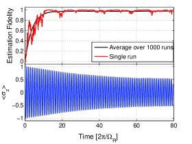
Figure 3: State estimation in the presence of classical noise. (a) Red line - Estimation fidelity for a single run (corresponding to Fig. 2), Black line - expected fidelity obtained by averaging 1000 runs. (b) Blue line - Rabi oscillations showing monotonic loss of coherence in the absence of unsharp measurements.

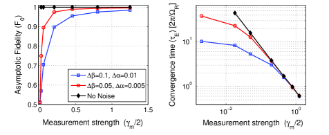
Figure 4: Effect of measurement strength on state estimation in environments with different noise strengths: diamonds - No noise, circles - $\Delta\beta=0.05,\Delta\alpha=0.005$, squares $\Delta\beta=0.1,\Delta\alpha=0.01$. (a) Asymptotic fidelity, $F_{0}$, as a function of measurement strength. (b) Convergence time, $\tau_{E}$, as a function of measurement strength. For the three weakest $\gamma_{m}$’s on the curves with noise, we plot in (a) the asymptotic fidelity and in (b) that time which it takes to reach a fraction $1-e^{-1}$ of that fidelity, even though the corresponding fidelity curves aren’t strictly exponential.

Each noise trajectory, $\alpha(t)$ and $\beta(t)$, is normalized so that their root-mean-square deviations are respectively one hundredth and one tenth of the drive field amplitude, $\Delta\alpha=0.005$ and $\Delta\beta=0.05$. We use the same measurement strength as before, but an observable $\hat{\mathbf{r}}\cdot\hat{\sigma}$ with a finite x- component: $\hat{\mathbf{r}}=(0.43,0,0.9)$, since the noise is expected to tip the Bloch vector out of the $yz$-plane.

Figure 2 displays the evolution of the expectation values (a) $\langle\hat{\sigma}_{x}\rangle$ and (b) $\langle\hat{\sigma}_{z}\rangle$ for the true state (black lines) and the estimate (red lines), again for a single run of the experiment. The amplitude of the Rabi oscillations, Fig. 2(b), although modulated by the noise, does not decrease permanently and the estimate succeeds in tracking both components. The red line in Fig. 3(a) shows the estimation fidelity corresponding to the single run of the experiment of Fig. (2). Despite the noise the state estimate quickly approaches the real state, although the fidelity does not converge completely to unity. Instead, it exhibits random excursions away from unity, which at long times are centered around an average, asymptotic value. To find this value we execute 1000 runs of the experiment with the same initial conditions and average over the resulting fidelities, leading to the black curve in Fig. 3(a). We’ve found empirically that this average fidelity $\bar{F}$ is well described by

$$\bar{F}(t)=F_{0}(1-e^{-t/\tau_{E}}).$$ (9)

In Eq. (9), $F_{0}$ is the asymptotic estimation fidelity and $\tau_{E}$ the estimation time. By fitting Eq. (9) to the simulated result we extract an estimation time of $\tau_{E}=3.7T_{R}$ and an asymptotic fidelity of $F_{0}=0.98$. For comparison the blue curve in Fig. 3(b) plots the result of an average over 1000 simulated runs of the experiment in the absence of measurements, but with the same noise source as in (a). It shows the decay of Rabi oscillations to about half full amplitude over the same time span due to the noise. Labelling $\tau_{R}$ the characteristic decay time of Rabi oscillations, we remark that Eq. (9) holds accurately only when $\tau_{m}\ll\tau_{R}$. For $\tau_{m}\gtrsim\tau_{R}$ the asymptotic approach is no longer simply exponential.

The results of Figs. 3 (a) and (b) taken together imply that in any single run of the experiment the state can be estimated at all times after convergence with an average of 98% fidelity, by a pure state $|\psi_{e}(t)\rangle$. On the other hand, in the absence of measurements the state would lose coherence due to the noise, and evolve into a statistical mixture as evidenced by the decay of Rabi oscillations of the ensemble average shown in Fig. 3 (b). This constitutes the main result of this letter. The fidelity can be operationally tested at the end of a run, by deducing from the state estimate the appropriate unitary rotations needed to place the system in the state $|\!\uparrow\rangle$, say, where it will then be detected with 98% probability. As such, the experimenter has maintained quantum control by monitoring of the state evolution, despite the noise.

Finally we study the effectiveness of the estimation process as a function of the measurement strength, $\gamma_{m}$, when noise is present. The simulations are repeated for different values of $\gamma_{m}$, and still choosing $\hat{\mathbf{r}}=(0.43,0,0.9)$ in each case. Figures 4(a) and (b) respectively plot the estimation fidelities and convergence times as a function of $\gamma_{m}$ for different noise strengths: diamonds - no noise, circles - $\Delta\beta=0.05,\Delta\alpha=0.005$, squares - $\Delta\beta=0.1,\Delta\alpha=0.01$. When noise is present, the asymptotic fidelity monotonically decreases as the measurement strength becomes weaker, and approaches $F_{0}=0.5$ as $\gamma_{m}\rightarrow 0$. This is consistent with the average fidelity obtained when taking random guesses for the state estimate. Simultaneously, the convergence time increases as the measurement becomes weaker, but plateaus to a finite value as $\gamma_{m}\rightarrow 0$. By contrast, in the absence of noise the fidelity always approaches $F_{0}=1$, but the convergence time increases indefinitely as the measurement strength weakens, as can be seen in Fig. 4(b).

The trends observed in Fig. 4 emphasize that the appropriate timescales need to be obeyed for the measurement scheme to work. The sequential measurement must be weak enough not to freeze the dynamics, but strong enough to enable a high fidelity estimate before the noise randomizes the system, i.e. $T_{R}\ll\tau_{m}\ll\tau_{R}$.

In conclusion, we remark that this study was carried out in a regime of comparatively strong noise, namely $\Omega_{R}/\Delta\beta=5\sim 10$. With stronger drive fields higher asymptotic fidelities can be expected for the same measurement strengths considered here. For example, we find that with $\Omega_{R}/\Delta\beta=100$, $\Omega_{R}/\Delta\alpha=1000$, $\Delta p=0.1$, $\hat{\mathbf{r}}=(0.43,0,0.9)$ ,that $F_{0}=0.999$ and $\tau=15.8T_{R}$. It is encouraging that the estimation procedure described here predicts finite estimation fidelity despite the presence of random classical noise. This opens the way for quantum control techniques that monitor wavefunction dynamics beyond the limitations set by decoherence processes in the absence of unsharp measurements.

References

- Chou et al. (2010) C. Chou, D. Hume, J. Koelemeij, D. Wineland, and T. Rosenband, Phys. Rev. Lett. 7, 070802 (2010).
- Palma et al. (1996) G. Palma, K. Suominen, and A. Ekert, Proc. Roy. Soc. London Ser. A 452, 567 (1996).
- Cywinski et al. (2008) L. Cywinski, R. Lutchyn, C. Nave, and S. Das Sarma, Phys. Rev. B 77, 174509 (2008).
- Busch et al. (1995) P. Busch, M. Grabowski, and J. Lahti, Operational Quantum Physics (Springer Verlag, Heidelberg, 1995).
- Audretsch et al. (2007) J. Audretsch, F. Klee, and T. Konrad, Physics Letters A 361, 212 (2007).
- Audretsch et al. (2001) J. Audretsch, T. Konrad, and A. Scherer, Phys. Rev. A 63, 052102 (2001).
- Belavkin V.P. (1989) Belavkin V.P., Lect. Notes Control Inf. Sci. 121, 245 (1989).
- Diosi et al. (2006) L. Diosi, T. Konrad, A. Scherer, and J. Audretsch, J. Phys. A: Math. Gen. 39, L575 (2006).
- Konrad et al. (2010) T. Konrad, A. Rothe, F. Petruccione, and L. Diosi, New. J. Phys. 12, 043038 (2010).
- Doherty et al. (1999) A. Doherty, S. Tan, A. Parkins, and D. Walls, Phys. Rev. A 60, 2380 (1999).
- Corney and Milburn (1998) J. Corney and G. Milburn, Phys. Rev. A 58, 2399 (1998).
- Audretsch et al. (2002a) J. Audretsch, T. Konrad, and A. Scherer, Phys. Rev. A 65, 033814 (2002a).
- Korotkov (2003) A. Korotkov, Phys. Rev. B 67, 235408 (2003).
- Oxtoby et al. (2008) N. Oxtoby, J. Gambetta, and H. Wiseman, Phys. Rev. B 77, 125304 (2008).
- Ritchie et al. (1991) N. Ritchie, J. Story, and R. Hulet, Phys. Rev. Lett. 66, 1107 (1991).
- Dixon et al. (2009) P. Dixon, D. Starling, A. Jordan, and J. Howell, Phys. Rev. Lett. 102, 173601 (2009).
- Hosten and Kwiat (2008) O. Hosten and P. Kwiat, Science 319, 787 (2008).
- Koksis et al. (2011) S. Koksis, B. Braverman, S. Ravets, M. Stevens, R. Mirin, L. Shalm, and A. Stenberg, Science 332, 1170 (2011).
- Silberfarb et al. (2005) A. Silberfarb, P. Jessen, and I. Deutsch, Phys. Rev. Lett. 95, 030402 (2005).
- Nielsen M.A. and Chuang (2002) Nielsen M.A. and I. Chuang, Quantum Computation and Quantum Information (Cambridge, UK, 2002).
- Audretsch et al. (2002b) J. Audretsch, L. Diósi, and T. Konrad, Phys. Rev. A 66, 022310(1 (2002b), e-print quant-ph/0201078.
- Misra and Sudarshan (1977) B. Misra and E. Sudarshan, J. Math. Phys. 18, 756 (1977).