On the Critical Delays of Mobile Networks under Lévy Walks and Lévy Flights

Abstract

Delay-capacity tradeoffs for mobile networks have been analyzed through a number of research work. However, Lévy mobility known to closely capture human movement patterns has not been adopted in such work. Understanding the delay-capacity tradeoff for a network with Lévy mobility can provide important insights into understanding the performance of real mobile networks governed by human mobility. This paper analytically derives an important point in the delay-capacity tradeoff for Lévy mobility, known as the critical delay. The critical delay is the minimum delay required to achieve greater throughput than what conventional static networks can possibly achieve (i.e., $O(1/\sqrt{n})$ per node in a network with $n$ nodes). The Lévy mobility includes Lévy flight and Lévy walk whose step size distributions parametrized by $\alpha\in(0,2]$ are both heavy-tailed while their times taken for the same step size are different. Our proposed technique involves (i) analyzing the joint spatio-temporal probability density function of a time-varying location of a node for Lévy flight and (ii) characterizing an embedded Markov process in Lévy walk which is a semi-Markov process. The results indicate that in Lévy walk, there is a phase transition such that for $\alpha\in(0,1)$, the critical delay is always $\Theta(n^{\frac{1}{2}})$ and for $\alpha\in[1,2]$ it is $\Theta(n^{\frac{\alpha}{2}})$. In contrast, Lévy flight has the critical delay $\Theta(n^{\frac{\alpha}{2}})$ for $\alpha\in(0,2]$.

I Introduction

Since the seminal work by Gupta and Kumar [1] on the capacity of wireless networks, delay and throughput tradeoffs for wireless networks have been extensively studied for various mathematical techniques, scheduling algorithms, channel models, mobility models and physical layer techniques. The work by Grossglauser and Tse [2] showed that the per-node throughput remains constant ($\Theta(1)$) when node mobility is used for communication. This result is surprising because Gupta and Kumar [1] had previously shown that the per-node throughput ($O(1/\sqrt{n})$) in wireless networks with no mobility diminishes as the number of nodes $n$ increases. This throughput gain is achieved at the cost of larger delays.

The amount of delay that a network needs to sacrifice to guarantee a given throughput has been studied under various mobility models [3, 4, 5]. In particular, Sharma et al. [6] studied the minimum delays required to achieve more per-node throughput than $\Theta(1/\sqrt{n})$ under various mobility models including i.i.d., random waypoint, random direction and Brownian motion. This minimum delay is called critical delay. However, although the work provides a nice framework for studying delay-capacity scaling for wireless networks under a family of random walk models, the practical values of these mobility models are limited. While these models are simple enough for mathematical tractability, they do not reflect realistic mobility patterns commonly exhibited in real mobile networks.

(a) Brownian motion

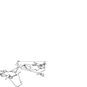
(b) Lévy mobility

(c) Random waypoint

Figure 1: Sample trajectories of (a) Brownian motion, (b) Lévy mobility and (c) random waypoint.

Humans are a major factor in mobile networks as most mobile nodes or devices (smartphones and cars) are carried or driven by humans. Recent studies [7, 8, 9] on human mobility show that step size distributions are heavy-tailed where a step is defined to be the straight line trip of a moving object (e.g., particles or humans) from one location to another without a directional change or pause. These mobility patterns are accurately modeled by Lévy process [10].

Lévy mobility is a random walk mobility whose step size distribution is parametrized by $\alpha\in(0,2]$ and is heavy-tailed except in the extreme case of $\alpha=2$. For $\alpha\in(0,2)$, the distribution is well approximated by a power-law distribution $1/z^{1+\alpha}$ where $z$ is a step size. For $\alpha=2$, the step size conforms to Gaussian distribution. Intuitively, such a random walk contains many short steps and a small yet significant number of exceptionally long steps. With different values of $\alpha$, the movement patterns of Lévy mobility models are widely different. Smaller $\alpha$ induces a larger number of long steps. This type of mobility patterns is significantly different from Brownian motion and random waypoint as illustrated in Fig. 1. In the literature, there are two types of Lévy mobility models for classification: Lévy flight and Lévy walk. In Lévy flight, every step takes a constant time irrespective of its step size and in Lévy walk, it takes a constant velocity. Lévy flight and Lévy walk can show the same pattern of traces but their time durations taken to have such traces are essentially different. Intuitively, Lévy flight can be easily slotted while Lévy walk is not.

Unfortunately, understanding tradeoffs between throughput and delay under Lévy mobility models is technically very challenging and underexplored. Unlike the other random walk models permitting mathematical tractability, the Lévy process is not very well understood mathematically despite significant studies on Lévy process in mathematics and physics. Thus, the conventional techniques [6, 5] used to study delay-capacity tradeoffs cannot be applied to Lévy mobility models, especially to Lévy walk which has high spatio-temporal correlation. In more specific, since Lévy walk is not eligible for discretization for Markovian analysis, its mathematical characteristics such as joint spatio-temporal probability density function (PDF) are hardly known. Due to such a difficulty, analyzing Lévy walk is generally considered to be very challenging.

Our main contribution is to analytically derive important tradeoffs between delay and capacity for both Lévy mobility models. An important point in this tradeoff is the “critical delay” which is the minimum delay for a mobile network to obtain a larger throughput than $\Theta(1/\sqrt{n})$. Our technique involves (i) analyzing the joint spatio-temporal PDF of a time-varying location of a node and the diffusion equation of the node for Lévy flight and (ii) characterizing an embedded Markov process inherent in Lévy walk which is a semi-Markov process. Since a different value of $\alpha$ induces a different mobility pattern, it also induces a different critical delay. Below we summarize our main results.

Mobility	$\alpha$	Critical Delay
Lévy walk	$\alpha\in(0,1)$	$\Theta(\sqrt{n})$
	$\alpha\in[1,2]$	$\Theta(n^{\alpha/2})$
Lévy flight	$\alpha\in(0,2]$	$\Theta(n^{\alpha/2})$

Given that many human mobility traces are shown to have values of $\alpha$ between 0.53 and 1.81 [7], according to our results, mobile networks assisted by human mobility have critical delays between $\Theta(n^{0.27})$ and $\Theta(n^{0.91})$. Note that our results give much more detailed prediction of the critical delay for such mobile networks depending on $\alpha$ while Brownian motion and random waypoint always show $\Theta(n)$ and $\Theta(n^{0.5})$ for their critical delays [6].

The rest of the paper is organized as follows. We first overview a list of related work in Section II and introduce our system model in Section III. More details of Lévy mobility model parameterized by $\alpha$ are described in Section IV, and the critical delays under Lévy flight and Lévy walk are investigated in Sections V and VI, respectively. Finally, we provide a high level interpretation of our main results in Section VII and concluding remarks in Section VIII.

II Related Work

Gupta and Kumar [1] showed that the per-node throughput of random wireless networks with $n$ static nodes scales as a function of $O(1/\sqrt{n})$ and proposed a scheme achieving $\Theta(1/\sqrt{n\log{n}})$. The result for static wireless networks was later enhanced to $\Theta(1/\sqrt{n})$ by exercising individual power control [11, 12]. Grossglauser and Tse [2] proved that a constant per-node throughput is achievable by using mobility when the nodes follow ergodic and stationary mobility models. This result disproved the conventional belief that node mobility can negatively impact network capacity as it causes connectivity breakup and channel quality degradation.

Many follow-up studies [13, 14, 15, 4, 3, 16, 17] have been devoted to understand, characterize and exploit the tradeoffs between throughput and delay. Especially, the delay required to obtain the constant throughput $\Theta(1)$ has been later studied under various mobility models [4, 18, 16, 17]. The studies provided that the delay to obtain $\Theta(1)$ of per-node throughput becomes $\Theta(n)$ for most mobility models such as i.i.d. mobility, random direction, random waypoint and Brownian motion models.

Another interesting question that has attracted researchers is what should be the minimum delay to achieve asymptotically higher throughput than $\Theta(1/\sqrt{n})$, the per-node throughput of static networks. This has been studied under the notion of critical delay [5, 6] for two families of random mobility models: hybrid random walk and random direction. The hybrid random walk model splits the network of size 1 with $n^{2\beta}$ cells and further splits a cell into $n^{1-2\beta}$ subcells for $\beta\in[0,1/2]$. Then, a node moves to a random subcell of an adjacent cell in every unit time slot. In this model, i.i.d. mobility corresponds to $\beta=0$ and random walk mobility corresponds to $\beta=1/2$. For any $\beta\in[0,1/2]$, critical delay is proved to be $\Theta(n^{2\beta})$. The random direction model chooses a random direction within $[0,2\pi]$ and moves to the selected direction with a distance of $n^{-\gamma}$ with a velocity $n^{-1/2}$ for $\gamma\in[0,1/2]$. In this model, random waypoint and Brownian motion are represented with $\gamma=0$ and $\gamma=1/2,$ respectively. The critical delay is proved to be $\Theta(n^{1/2+\gamma})$.

III Model Description

III-A System Model

We consider a wireless mobile network indexed by $n$, where in the $n$-th network, $n$ nodes are distributed uniformly on a completely wrapped-around square $\mathcal{S}(n)$ whose width and height scale as $\sqrt{n}$ and the density is fixed to 1 with increasing $n.$ Without loss of generality, we set the width and the height of the square $\mathcal{S}(n)$ as $\sqrt{n}$. We assume that all nodes are homogeneous in that each node generates data with the same intensity to a per-source destination. The packet generation process at each node is assumed to be independent of node mobility.

A source-to-destination packet can be delivered by either direct one-hop transmission or over multiple hops, say $k$ hops, using relay nodes. We call it $k$-hop relay transmission. We assume that all nodes can serve as relay nodes for other source nodes and the nodes serving as relay nodes can only forward packets rather than replicating packets (not to overproduce the same packets in the network).

To model interference in wireless networks, we use the protocol model as in [1], under which nodes transmit packet successfully at a constant rate $W$ bits/sec, if and only if the following is met: let $\bm{X}_{i}(t)\,(\in\mathbb{R}^{2})$ denote the location of node $i\,(i=1,\ldots,n)$ at time $t\,(\geq 0)$. For a transmitter $i$, a receiver $j$ and every other node $k\neq i,j$ transmitting simultaneously,

$$d(\bm{X}_{k}(t),\bm{X}_{j}(t))\geq(1+\Delta)\,d(\bm{X}_{i}(t),\bm{X}_{j}(t)),$$

where $d(\bm{x},\bm{y})$ denotes the Euclidean distance between locations $\bm{x},\bm{y}\in\mathbb{R}^{2}$, and $\Delta$ is some positive number.

A packet can be delivered through a scheduling scheme which consists of replication or forwarding. We assume that only source nodes replicate packets and all other relay nodes forward them. As the names imply, replication copies a packet and the packet transmitter keeps the packet, whereas in forwarding the transmitter does not keep the original packet after successful transmission. This selective replication and forwarding depending on the node type are often applied to suppress the overflow of redundant packets in the network. Packets are delivered in two ways: neighbor capture and multi-hop capture. In neighbor capture, using mobility, relay or source nodes are located within the communication range of the destination. In the multi-hop capture, a source establishes a multi-hop path to the destination and delivers the packets over the path. We assume a fluid packet model [19] so that the delivery can occur immediately even in the case of multi-hop capture because the transmission delay is negligible compared to the delay from node mobility. We denote by $\Pi$ the class of all scheduling schemes conforming the descriptions above.

III-B Performance Metrics

The primary performance metric in many networking systems is per-node throughput measured by the long-term average of received packets aggregated over nodes:

Definition 1 (Per-node throughput)

Let $\lambda_{\pi}(n)$ denote the per-node throughput in the $n$-th network under a scheduling scheme $\pi\in\Pi$. It is then given by

$$\lambda_{\pi}(n)\triangleq\liminf_{t\rightarrow\infty}\frac{1}{n}\sum_{i=1}^{n}\frac{\lambda_{\pi:i}(t)}{t},$$

where $\lambda_{\pi:i}(t)$ is the total number of bits received at a destination node $i$ up to time $t$ under $\pi$.

Another important metric is average delay:

Definition 2 (Average delay)

Let $D_{\pi}(n)$ denote the average delay in the $n$-th network under a scheduling scheme $\pi\in\Pi$. It is then given by

$$D_{\pi}(n)\triangleq\lim_{k\rightarrow\infty}\frac{1}{n}\sum_{i=1}^{n}\frac{1}{k}\sum_{j=1}^{k}D_{\pi:(i,j)},$$

where $D_{\pi:(i,j)}$ is the individual packet delay that a packet $j$ experiences to arrive at a destination node $i$ from its source node under $\pi$.

We give special attention to the notion of critical delay, first introduced in [6]:

Definition 3 (Critical delay)

The critical delay in the $n$-th network, denoted by $C_{\Pi}(n)$, is the minimum average delay that must be tolerated under a given mobility model to achieve a per-node throughput of $\omega(1/\sqrt{n})$, i.e.,

$$C_{\Pi}(n)\triangleq\inf_{\{\pi\in\Pi:\lambda_{\pi}(n)=\omega(1/\sqrt{n})\}}D_{\pi}(n).$$

Per-node throughput $\Theta(1/\sqrt{n})$ is achievable by a scheduling scheme in static multi-hop networks [1]. Since node mobility can increase per-node throughput at the cost of larger delay, the critical delay quantifies the amount of delay that a network should sacrifice to achieve the guaranteed “baseline” per-node throughput. It can be used as a simple, yet useful metric for a mobility model, representing how sensitive the delay is to increase per-node throughput.

Computing critical delay consists of multiple steps. We start by following the initial step in [5, 6] which connects critical delay to the first exit time. Let $\mathcal{D}(n)$ denote a disc within the square $\mathcal{S}(n)$ whose radius scales as $\Theta(\sqrt{n})$. Critical delay can simply be regarded as the maximum time duration that a node cannot exit from the disc $\mathcal{D}(n)$ with probability approaching 1 as $n$ goes to $\infty$. In our extended network model, the average distance from a source node to a destination node is $\Theta(\sqrt{n})$ when they are uniformly distributed on $\mathcal{S}(n)$. Therefore, if nodes travel up to a distance $O(\sqrt{n})$, for a certain time duration, the distance between a source or a relay and a destination still remains $\Theta(\sqrt{n})$ on average which results in $O(1/\sqrt{n})$ per-node throughput (see Lemma 1). Thus, it is obvious that a network aiming at obtaining $\omega(1/\sqrt{n})$ per-node throughput must allow a delay which is no less than the maximum time duration that the first exit of a node from the disc $\mathcal{D}(n)$ does not occur with probability approaching 1. This insight can be formally described with the notion of the first exit time:

Definition 4 (First exit time)

Let $\bm{X}_{i}(0)=\bm{x}$. The first exit time for a disc of a radius $r$, denoted by $T(r)$, is defined as

$$T(r)\triangleq\inf\{t\geq 0:\bm{X}_{i}(t)\notin B(\bm{x},r)\},$$

where $B(\bm{x},r)$ denotes the set of points $\bm{y}$ in $\mathcal{S}(n)$ such that $d(\bm{x},\bm{y})\leq r$.

Without loss of generality, we set the radius of the disc $\mathcal{D}(n)$ as $c_{d}\sqrt{n}$ where $c_{d}$ is a constant in the range $(0,1/2)$. Then, critical delay $C_{\Pi}(n)$ can be obtained by

$$C_{\Pi}(n)=\sup\left\{t(n):\lim_{n\rightarrow\infty}\text{P}\{T(c_{d}\sqrt{n})>t(n)\}=1\right\}.$$

Lemma 1 ([5, 1])

Suppose that on average each packet is relayed over a total distance no less than $\Theta(\sqrt{n})$ in an extended network model. Then, the per-node throughput $\lambda(n)$ scales as $O(1/\sqrt{n})$.

IV Mobility Models: Lévy Flight and Lévy Walk

In this section, we formally define Lévy mobility model: Lévy flight and Lévy walk.

Lévy flight and Lévy walk processes are treated separately in the literature [20, 21, 22]. Lévy flight takes a constant time for any step irrespective of its step size, whereas Lévy walk takes a constant velocity for every step. Thus, in Lévy walk, the time taken for each step is proportional to the step size. The distinction between Lévy flight and Lévy walk is often made based on the speeds of their actual processes. Lévy flight is a “fast” mobility model which can reach its next destination in a constant time no matter how far it is. In a similar context, Lévy walk falls under a “slow” mobility model. An experimental velocity model suggested as a function of step size in [7] verifies that a human mobility lies in between Lévy flight and Lévy walk. For convenience, we use Lévy mobility model to indicate both of Lévy flight and Lévy walk, unless explicitly stated.

Let $Z$ be a random variable denoting the step size under Lévy mobility model. Then, $Z$ is generated from a random variable $\dot{Z}$ having the Lévy $\alpha$-stable distribution [23] by the relation $Z=|\dot{Z}|$. The PDF of $\dot{Z}$ is give by

$$f_{\dot{Z}}(z)=\frac{1}{2\pi}\int_{-\infty}^{\infty}e^{-izt}\varphi_{\dot{Z}}(t)\,\text{d}t,$$ (1)

where $\varphi_{\dot{Z}}(t)\triangleq\text{E}[e^{it\dot{Z}}]$ is the characteristic function of $\dot{Z}$ and is given by $\varphi_{\dot{Z}}(t)=e^{-|ct|^{\alpha}}$. Here, $|c|>0$ is a scale factor which is a measure of the width of the distribution, and $\alpha\in(0,2]$ is a distribution parameter and specifies the shape (i.e., heavytail-ness) of the distribution. The step size $Z$ for $\alpha\in(0,1)$ has infinite mean and variance, while $Z$ for $\alpha\in[1,2)$ has finite mean but infinite variance. For $\alpha=2$, the Lévy $\alpha$-stable distribution reduces to a Gaussian distribution with zero mean and variance $\sigma^{2}=2c^{2}$, and consequently the step size $Z$ has finite mean and variance.

Due to the complex form of the distribution, the Lévy $\alpha$-stable distribution for $\alpha\in(0,2)$ is often given as a power-law type of asymptotic form, closely approximating the tail part of the distribution [23]:

$$f_{\dot{Z}}(z)\sim\frac{1}{|z|^{1+\alpha}}.$$ (2)

For mathematical tractability, in our analysis we use the asymptotic form (2) instead of the exact form (1) for $\alpha\in(0,2)$ while using the exact form (1) for $\alpha=2$. The form (2) is known to closely approximate (1) and several papers in mathematics and physics, e.g., [20, 24], analyze Lévy mobility using form (2). For the range of $Z$, since we use the extended network model, the step size $Z$ is assumed to have a lower bound at 1 and an upper bound at $\sqrt{n}$, i.e., $\text{P}\left\{1\leq Z\leq\sqrt{n}\right\}=1$. Thus, the complementary cumulative distribution function (CCDF) of $Z$ becomes $\text{P}\{Z>z\}=1$ for $z<1$ and $\text{P}\{Z>z\}=0$ for $z\geq\sqrt{n}$. For $z\in[1,\sqrt{n})$, we have

$$\text{P}\{Z\!>\!z\} \!=\!\begin{cases}c(n)\cdot\!\big{(}\frac{1}{z^{\alpha}}\!-\!\frac{1}{(\sqrt{n})^{\alpha}}\big{)}&\text{for }\alpha\in(0,2),\\ c(n)\cdot\!\big{(}\mathrm{erf}(\frac{\sqrt{n}}{\sqrt{2}\sigma})\!-\!\mathrm{erf}(\frac{z}{\sqrt{2}\sigma})\big{)}&\text{for }\alpha=2.\end{cases}$$ (3)

Here, $\mathrm{erf}(\cdot)$ is the error function defined as $\mathrm{erf}(x)\triangleq\frac{2}{\sqrt{\pi}}\int_{0}^{x}\exp(-t^{2})\,\text{d}t$, and $c(n)$ is defined as

$$c(n)\triangleq\begin{cases}(1-\frac{1}{(\sqrt{n})^{\alpha}})^{-1}&\text{ for }\alpha\in(0,2),\\ (\mathrm{erf}(\frac{\sqrt{n}}{\sqrt{2}\sigma})-\mathrm{erf}(\frac{1}{\sqrt{2}\sigma}))^{-1}&\text{ for }\alpha=2.\end{cases}$$

Note that as $n$ goes to $\infty$, the CCDF $\text{P}\{Z>z\}$ for $z\geq 1$ goes to $1/z^{\alpha}$ for $\alpha\in(0,2)$.

In our analysis, we use the following assumptions on the Lévy mobility model: (A1) the time taken for each step in the Lévy flight is set to 1, and (A2) the velocity taken for each step in Lévy walk is set to 1. Note that as long as these two metrics are constant, the scaling property of critical delay remains the same, which justifies our assumptions.

V Critical Delay Analysis for Lévy Flight

In this section, we will show that the critical delay $C_{\Pi}(n)$ under Lévy flight with a distribution parameter $\alpha\in(0,2]$ scales as $\Theta(n^{\frac{\alpha}{2}})$ (Theorem 1). In Section V-A, we explain technical challenges and our approach for proving Theorem 1. In Section V-B, we prove Theorem 1 by showing that the upper bound on $C_{\Pi}(n)$ scales as $O(n^{\frac{\alpha}{2}})$ (Lemma 3), and that the lower bound on $C_{\Pi}(n)$ scales as $\Omega(n^{\frac{\alpha}{2}})$ (Lemma 4).

V-A Technical Approach

We begin with deriving a relation between the first exit time of a 2-dimensional random process and the one for its 1-dimensional projected process. We then describe trapping phenomenon in a diffusion process that have a direct connection to the first exit time of a 1-dimensional random process.

It is clear from Definition 4 that the statistical proprieties of the first exit time do not depend on the choice of node index $i$. Thus, we omit the node index $i$ in the rest of the paper. Denote $\bm{X}(t)=(X_{x}(t),X_{y}(t))$ and consider the projected processes $\{X_{x}(t)\}_{t\geq 0}$ and $\{X_{y}(t)\}_{t\geq 0}$ onto $x$-axis and $y$-axis, respectively. We define for the projected processes the first exit time similarly to Definition 4:

$$T_{x}(r) \triangleq\inf\left\{t\geq 0:|X_{x}(t)-X_{x}(0)|\geq r\right\},$$

$$T_{y}(r) \triangleq\inf\left\{t\geq 0:|X_{y}(t)-X_{y}(0)|\geq r\right\}.$$

Since the event $\{|X_{x}(t)-X_{x}(0)|\geq r\}$ implies the event $\{d(\bm{X}(t),\bm{X}(0))\geq r\}$, we obtain

$$\text{P}\{T_{x}(r)\leq t\}\leq\text{P}\{T(r)\leq t\}.$$ (4)

In addition, it is clear that

$$\text{P}\{T(r)\leq t\} \leq\text{P}\{T_{x}(r/\sqrt{2})\leq t\text{ or }T_{y}(r/\sqrt{2})\leq t\}$$

$$\leq 2\,\text{P}\{T_{x}(r/\sqrt{2})\leq t\},$$ (5)

where the second inequality comes from the union bound and the symmetry of node motion. Combining (4) and (V-A), we have for all $t\geq 0$,

$$\text{P}\{T_{x}(r)\leq t\} \leq\text{P}\{T(r)\leq t\}\leq 2\,\text{P}\{T_{x}(r/\sqrt{2})\leq t\}.$$ (6)

Our technical approach is mainly based on (6), and is to bound the first exit time distribution for 2-dimensional Lévy flight by the one for the corresponding 1-dimensional projected process $\{X_{x}(t)\}_{t\geq 0}$. We henceforth study the first exit time distribution for the process $\{X_{x}(t)\}_{t\geq 0}$.

The first exit time analysis for 1-dimensional random processes has been intensively studied in physics and mathematics, e.g., [25]. Specifically, trapping phenomenon (of a diffusing particle) in physics and its related theories have a direct connection to our first exit time problem as explained in the following: consider a particle that diffuses in a finite interval $[0,2r]\,(\subset\mathbb{R})$ having trapping boundaries at $x=0,2r$. Let $L(t)\,(\in\mathbb{R})$ be a random variable denoting the location of the particle at time $t$. The particle is assumed to be initially located at $L(0)=r$, and eventually it is trapped at either of both boundaries with probability 1. Upon the particle is trapped, it disappears in the interval. We call the state of the particle survival state until the particle is trapped and disappears. By convention, we let $L(t)\triangleq\varnothing$ if the particle is not in survival state at time $t$. If we assume $X_{x}(0)=L(0)\,(=r)$, then $X_{x}(t)$ and $L(t)$ for $t>0$ are related as follows:

$$\begin{split}L(t)\stackrel{{\scriptstyle\text{d}}}{{=}}\begin{cases}X_{x}(t)&\text{ if }t<T_{x}(r),\\ \varnothing&\text{ if }t\geq T_{x}(r),\end{cases}\end{split}$$ (7)

where $\stackrel{{\scriptstyle\text{d}}}{{=}}$ denotes “equal in distribution”. Hence, we have from (7) that

$$\text{P}\{T_{x}(r)\leq t\}=\text{P}\{L(t)=\varnothing\}.$$ (8)

That is, the survival time of a particle in the trapping model has the same distribution as the first exit time $T_{x}(r)$ of a node under Lévy flight.

The technical approach for analyzing the critical delay in the literature is as follows. In the case of Brownian motion, there are two general techniques in studying the critical delay. One is to discretize mobility and then apply a Markovian analysis [6]. The other is to use a continuous mobility model and solve a diffusion equation to obtain a joint spatio-temporal PDF of a time-varying location of a node [5]. The latter enables one to obtain the distribution of $L(t)$ whose spatial derivative is often referred to as occupation probability. The occupation probability of Brownian motion can be decomposed to find the components constituting it. From this decomposition process, we find that there is a dominating term which characterizes the limiting behavior of the first exit time distribution.

In the case of Lévy flight, the joint spatio-temporal PDF has a similar form to that of Brownian motion. In addition, the occupation probabilities and the first exit time distributions for Brownian motion and Lévy flight have similar structures in the aspect of the dominating terms. Hence, by identifying and characterizing the dominating term for Lévy flight, we can obtain the critical delay under Lévy flight.

V-B Analysis

In this subsection, we provide the detailed result for the critical delay under Lévy flight. Our main result is derived by following three steps: (i) the occupation probability is obtained from the solution of a differential equation that governs the movement of a particle. (ii) From the occupation probability, we obtain the survival probability (which will be defined later), which in turn yields the first exit time distribution. (iii) By investigating the limiting behavior of the first exit time distribution, we can finally obtain the order of the critical delay.

Step 1: Let $P(x,t)\triangleq\frac{\text{d}}{\text{d}x}\text{P}\{L(t)\leq x\}$. Intuitively, $P(x,t)$ represents probability that the particle is located at $x$ at time $t$. We call $P(x,t)$ the occupation probability, and it has the following properties:

• (P1) $\lim_{t\to\infty}P(x,t)=0~{}\forall x\in\mathbb{R}.$

• (P2) $\int_{0}^{2r}P(x,0)\,\text{d}x=\text{P}\{L(0)=r\}=1$.

• (P3) $\int_{0}^{2r}P(x,t)\,\text{d}x\leq 1~{}\forall t>0$.

• (P4) $P(0,t)=P(2r,t)=0~{}\forall t\geq 0$.

• (P5) Since $P(x,0)$ is a PDF having a support $\{r\}$, we have $P(x,0)=\delta_{x,r}$, where $\delta_{x_{1},x_{2}}$ denotes the Kronecker delta which is defined to be 1 if $x_{1}=x_{2}$ and 0 otherwise.

To be precise, $P(x,t)$ for $t>0$ could not be a PDF due to (P3). However, the function obtained by normalizing $P(x,t)$ with the integral $\int_{0}^{2r}P(x,t)\,\text{d}x$, denoted by $\bar{P}(x,t)$, becomes a PDF for a finite time $t$. We call $\bar{P}(x,t)$ the joint spatio-temporal PDF at location $x$ and time $t$.

In the first step, we obtain the occupation probability $P(x,t)$ for the process $\{L(t)\}_{t\geq 0}$. For this, we need to characterize the associated 1-dimensional process $\{X_{x}(t)\}_{t\geq 0}$. We first consider the case of $\alpha\in(0,2)$ and summarize the result in the following lemma.

Lemma 2

Suppose that $\{\bm{X}(t)\}_{t\geq 0}$ is 2-dimensional Lévy flight with a distribution parameter $\alpha\in(0,2)$. Then, as $n$ goes to $\infty$, the projected process onto $x$-axis $\{X_{x}(t)\}_{t\geq 0}$ approaches to 1-dimensional Lévy flight having the same distribution parameter $\alpha$. It holds for the process $\{X_{y}(t)\}_{t\geq 0}$.

Proof: Let $Z_{i}$ and $\theta_{i}\,(i=1,2,\ldots)$ be random variables denoting the $i$-th step size and direction of the process $\{\bm{X}(t)\}_{t\geq 0}$, respectively. Then, $\bm{X}(t)$ for $t=1,2,\ldots$ can be expressed as

$$\bm{X}(t) =(X_{x}(t),X_{y}(t))$$

$$=\bm{X}(0)+\left(\sum_{i=1}^{t}Z_{i}\cos\theta_{i},\,\sum_{i=1}^{t}Z_{i}\sin\theta_{i}\right).$$ (9)

We will show that, as $n$ goes to $\infty$, arbitrary step size of the projected processes (i.e., $Z_{i}|\cos\theta_{i}|$ and $Z_{i}|\sin\theta_{i}|$) has a power-law type CCDF with an exponent $\alpha$, i.e., for $z\geq 1$,

$$\begin{split}\lim_{n\to\infty}\text{P}\{Z_{i}|\cos\theta_{i}|>z\}&=\lim_{n\to\infty}\text{P}\{Z_{i}|\sin\theta_{i}|>z\}\\ &=\frac{c^{\star}}{z^{\alpha}},\end{split}$$ (10)

where $c^{\star}\triangleq\frac{2}{\pi}\int_{0}^{\frac{\pi}{2}}(\cos\vartheta)^{\alpha}\text{d}\vartheta$. Since the projected processes take a constant time for every step irrespective of step size, the property in (10) proves the lemma.

Now we prove (10). By conditioning on the values of the random variable $\theta_{i}\sim\text{Uniform}[0,2\pi]$, we can rewrite the CCDF of $Z_{i}|\cos\theta_{i}|$ as

$$\text{P}\{Z_{i}|\cos\theta_{i}|>z\} =\int_{0}^{2\pi}\text{P}\{Z_{i}|\cos\theta_{i}|>z\,|\,\theta_{i}=\vartheta\}\text{d}F_{\theta_{i}}(\vartheta)$$

$$=\frac{1}{2\pi}\int_{0}^{2\pi}\text{P}\{Z_{i}|\cos\vartheta|>z\}\text{d}\vartheta$$

$$=\frac{2}{\pi}\int_{0}^{\frac{\pi}{2}}\text{P}\{Z_{i}\cos\vartheta>z\}\text{d}\vartheta,$$ (11)

where the last two equalities come from the independence of the random variables $Z_{i}$ and $\theta_{i}$, and the symmetry of the function $|\cos\vartheta|$, respectively. Using (3), the probability $\text{P}\{Z_{i}\cos\vartheta>z\}$ in (2) can be obtained for $\vartheta\in[0,\frac{\pi}{2}]$ as

$$\text{P}\{Z_{i}\cos\vartheta>z\}$$

$$=\begin{cases}c(n)\cdot\big{(}(\frac{\cos\vartheta}{z})^{\alpha}-(\frac{1}{\sqrt{n}})^{\alpha}\big{)}&\text{for }\vartheta\in[0,\cos^{-1}(\frac{z}{\sqrt{n}})),\\ 0&\text{for }\vartheta\in[\cos^{-1}(\frac{z}{\sqrt{n}}),\frac{\pi}{2}].\end{cases}$$

Hence, the CCDF $\text{P}\{Z_{i}|\cos\theta_{i}|>z\}$ is given by

$$\begin{split}\text{P}\{Z_{i}|\cos\theta_{i}|>z\}&=\frac{2c(n)}{\pi z^{\alpha}}\int_{0}^{\cos^{-1}(\frac{z}{\sqrt{n}})}(\cos\vartheta)^{\alpha}\text{d}\vartheta\\ &\qquad-\frac{2c(n)}{\pi(\sqrt{n})^{\alpha}}\cos^{-1}\left(\frac{z}{\sqrt{n}}\right).\end{split}$$ (12)

Noting $\lim_{n\to\infty}c(n)=1$ and $\lim_{n\to\infty}\cos^{-1}\left(\frac{z}{\sqrt{n}}\right)=\frac{\pi}{2}$, we have from (12) that

$$\lim_{n\to\infty}\text{P}\{Z_{i}|\cos\theta_{i}|>z\} =\frac{2}{\pi z^{\alpha}}\int_{0}^{\frac{\pi}{2}}(\cos\vartheta)^{\alpha}\text{d}\vartheta=\frac{c^{\star}}{z^{\alpha}}.$$

Since $|\sin\theta_{i}|\stackrel{{\scriptstyle\text{d}}}{{=}}|\cos\theta_{i}|$ for $\theta_{i}\sim\text{Uniform}[0,2\pi]$, we have

$$\text{P}\{Z_{i}|\sin\theta_{i}|>z\} =\text{P}\{Z_{i}|\cos\theta_{i}|>z\},$$

which completes the proof. $\square$

Motivated by Lemma 2 and (7), we study the occupation probability for 1-dimensional Lévy flight with $\alpha\in(0,2)$ in a finite interval $[0,2r]$ having trapping boundaries. For mathematical tractability, our study in this subsection assumes continuous limit where the scale factor $|c|$ in (1) approaches to zero. Then, the occupation probability $P(x,t)$ for $\alpha\in(0,2)$ is governed by the following fractional Fokker-Planck equation [22, Eq. (22)], [26, Eq. (28)]:

$$\frac{\partial P(x,t)}{\partial t}=F\frac{\partial^{\alpha}P(x,t)}{\partial|x|^{\alpha}},$$ (13)

where $F\,(=F_{\alpha}>0)$ is a generalized diffusion coefficient and $\frac{\partial^{\alpha}}{\partial|x|^{\alpha}}$ is the Riesz-Feller derivative of fractional order $\alpha$ [27]. We next consider the case of $\alpha=2$. In this case, as the scale factor $|c|$ approaches to zero, the 2-dimensional Lévy flight converges to a Wiener process which mathematically models a continuous movement of Brownian motion. Since 1-dimensional projected process of 2-dimensional Brownian motion is also Brownian motion [5], the occupation probability for $\alpha=2$ is governed by the normal diffusion equation where the spatial derivative of order $\alpha$ with $\alpha\in(0,2)$ in (13) is replaced by the second order derivative with $\alpha=2$ [25]. Therefore, with continuous limit, the occupation probability $P(x,t)$ for $\alpha\in(0,2]$ can be described by the differential equation in (13). Through Appendix A, we show that the order of the critical delay under Lévy flight does not change with continuous limit.

Applying the standard method of separation of variables gives the solution of (13) as follows:

$$P(x,t)=\sum_{i=1}^{\infty}h_{i}\psi_{i}(x)\exp\left(\lambda_{i}Ft\right).$$ (14)

Here, $h_{i}\,(i=1,2,\ldots)$ are determined from the initial condition $P(x,0)=\delta_{x,r}$ (as shown in (P5)) and are given by $h_{i}=\psi_{i}(r)$. The functions $\psi_{i}(x)$ and the constants $\lambda_{i}$ can be obtained from the solutions of the problem $\mathfrak{D}[\psi_{i}(x)]=\lambda_{i}\psi_{i}(x)$ for the operator $\mathfrak{D}\triangleq\frac{\text{d}^{\alpha}}{\text{d}|x|^{\alpha}}$, and are called eigenfunctions and eigenvalues of $\mathfrak{D}$, respectively. Without loss of generality, we assume that $\lambda_{i}$ are arranged as $|\lambda_{1}|<|\lambda_{2}|<\cdots$.

Step 2: Let $S(t)\triangleq\text{P}\{L(t)\neq\varnothing\}$. Intuitively, $S(t)$ represents probability that the particle has not hit any trapping boundary by time $t$. We call $S(t)$ the survival probability. The survival probability can be obtained from the occupation probability $P(x,t)$ by $S(t)=\int_{0}^{2r}P(x,t)\,\text{d}x$. Thus, from (14), the survival probability is given by

$$S(t)=\sum_{i=1}^{\infty}\psi_{i}(r)\int_{0}^{2r}\psi_{i}(x)\,\text{d}x\exp\left(\lambda_{i}Ft\right).$$ (15)

The first exit time distribution $\text{P}\{T_{x}(r)\leq t\}$ can be obtained from the survival probability $S(t)$ through the following relation:

$$\text{P}\{T_{x}(r)\leq t\} =\text{P}\{L(t)=\varnothing\}=1-S(t).$$ (16)

Here, the first equality comes from (8) and the second equality comes from the definition of $S(t)$. By combining (15) and (16), we obtain the first exit time distribution in terms of the eigenfunctions $\psi_{i}(x)$ and the eigenvalues $\lambda_{i}$ as follows:

$$\text{P}\{T_{x}(r)\leq t\} =1-\sum_{i=1}^{\infty}\!\psi_{i}(r)\!\int_{0}^{2r}\!\!\!\psi_{i}(x)\text{d}x\exp\left(\lambda_{i}Ft\right).$$ (17)

For $\alpha=2$, the eigenfunctions and the eigenvalues in (17) can be obtained from the boundary conditions $P(0,t)=P(2r,t)=0~{}\forall t\geq 0$ (as shown in (P4)), and are given by $\psi_{i}(x)=\sqrt{\frac{1}{r}}\sin\left(\frac{i\pi x}{2r}\right)$ and $\lambda_{i}=-\left(\frac{i\pi}{2r}\right)^{2}$, respectively [25]. For $\alpha\in(0,2)$, Gitterman [26] provided a solution of (13) whose eigenfunctions and eigenvalues are given by $\psi_{i}(x)=\sqrt{\frac{1}{r}}\sin\left(\frac{i\pi x}{2r}\right)$ and $\lambda_{i}=-\left(\frac{i\pi}{2r}\right)^{\alpha}$, respectively. Thus, under Lévy flight with $\alpha\in(0,2]$, the first exit time distribution can be expressed as an infinite series of exponential functions as follows:

$$\text{P}\{T_{x}(r)\leq t\}=1-\sum_{i=1}^{\infty}\eta_{i}\exp\left(-\frac{\rho_{i}}{r^{\alpha}}t\right),$$ (18)

where $\eta_{i}\triangleq\frac{2\{1-\cos(i\pi)\}}{i\pi}\sin\left(\frac{i\pi}{2}\right)$ and $\rho_{i}\triangleq F(\frac{i\pi}{2})^{\alpha}$.

As will be shown later in the proof of Lemmas 3 and 4, the smallest (i.e., dominant) decay rate in the exponential functions in (14) (i.e., $|\lambda_{1}|$) determines the limiting behavior of the first exit time distribution. That is, the smallest decay rate characterizes the critical delay under Lévy flight. The solutions in [25, 26] show that the dominant decay rate $|\lambda_{1}|$ scales as $\Theta(r^{-\alpha})$ for $\alpha\in(0,2]$.

Step 3: We are now ready to derive the main result of this subsection. By using the closed-form expression for $\text{P}\{T_{x}(r)\leq t\}$ in (18), we investigate the order of the critical delay, stated in Lemmas 3 and 4.

Lemma 3 (Upper bound for Lévy flight)

Suppose that under Lévy flight with a distribution parameter $\alpha\in(0,2]$, the time $t\triangleq\hat{t}(n)$ in $\text{P}\{T(c_{d}\sqrt{n})>t\}$ scales as $\Theta(n^{\frac{\alpha}{2}+\epsilon})$ for an arbitrary $\epsilon>0$. Then, we have

$$\lim_{n\to\infty}\text{P}\{T(c_{d}\sqrt{n})>\hat{t}(n)\}=0,$$

which shows that the critical delay $C_{\Pi}(n)$ under Lévy flight scales as $O(n^{\frac{\alpha}{2}})$.

Proof: We will prove this lemma by showing that $\lim_{n\to\infty}\text{P}\{T_{x}(c_{d}\sqrt{n})\leq\hat{t}(n)\}=1$. Then, by substituting $r=c_{d}\sqrt{n}$ and $t=\hat{t}(n)$ into (6) and taking a limit to $n$, we obtain

$$1 =\lim_{n\to\infty}\text{P}\{T_{x}(c_{d}\sqrt{n})\leq\hat{t}(n)\}$$

$$\leq\lim_{n\to\infty}\text{P}\{T(c_{d}\sqrt{n})\leq\hat{t}(n)\}.$$

That is, $\lim_{n\to\infty}\text{P}\{T(c_{d}\sqrt{n})\leq\hat{t}(n)\}=1$, or equivalently, $\lim_{n\to\infty}\text{P}\{T(c_{d}\sqrt{n})>\hat{t}(n)\}=0$, which proves the lemma.

First, consider the case of $\alpha=2$. We substitute $r=c_{d}\sqrt{n}$ and $t=\hat{t}(n)$ into (18). Then, the series on the right-hand side of (18) becomes a function of $n$, and (for notational convenience) we let

$$\text{P}\{T_{x}(c_{d}\sqrt{n})\leq\hat{t}(n)\} =1-\sum_{i=1}^{\infty}\eta_{i}\exp\left(-\frac{\rho_{i}}{(c_{d})^{2}n}\hat{t}(n)\right)$$

$$\triangleq 1-\hat{S}(n).$$

We now need to take a limit to $\hat{S}(n)$. To validate the interchange of the order of limit and summation, we will show that there exists a constant $\hat{n}\in\mathbb{N}$ such that the infinite series $\hat{S}(n)$ converges uniformly on $\hat{\mathcal{D}}\triangleq[\hat{n},\infty)$. The uniform convergence will be shown by using the well-known Weierstrass $M$ test [28].

Since $\hat{t}(n)=\Theta(n^{1+\epsilon})$, there exist constants $\hat{n}\in\mathbb{N}$ and $\hat{c}>0$ such that

$$\hat{t}(n)\geq\hat{c}n^{1+\epsilon}\quad\text{ for all }n\geq\hat{n}.$$ (19)

Let $\hat{m}\triangleq F(\pi/2c_{d})^{2}\hat{c}(\hat{n})^{\epsilon}\,(>0)$. Then, the $i$-th function of the series $\hat{S}(n)$ is bounded by a constant $\hat{M}_{i}\triangleq\frac{4}{\pi}\{\exp(-\hat{m})\}^{i}$ for all $n\geq\hat{n}$ as follows:

$$\bigg{|}\eta_{i}\exp\left(-\frac{\rho_{i}}{(c_{d})^{2}n}\hat{t}(n)\right)\bigg{|} \leq\frac{4}{\pi}\exp\left(-\frac{\rho_{i}}{(c_{d})^{2}n}\hat{c}n^{1+\epsilon}\right)$$

$$\leq\frac{4}{\pi}\exp\left(-\frac{Fi(\pi)^{2}}{4(c_{d})^{2}}\hat{c}(\hat{n})^{\epsilon}\right)$$

$$=\hat{M}_{i}.$$

Here, the first inequality comes from the bounds $|\eta_{i}|\leq\frac{4}{\pi}~{}\forall i\in\mathbb{N}$ and (19), and the second inequality comes from the bounds $i^{2}\geq i~{}\forall i\in\mathbb{N}$ and $n^{\epsilon}\geq(\hat{n})^{\epsilon}~{}\forall n\geq\hat{n}$. Note that the series $\sum_{i=1}^{\infty}\hat{M}_{i}$ converges since it is a geometric series with a common ratio $\exp(-\hat{m})\in(0,1)$. Since the target of the functions is a complete normed vector space, the infinite series $\hat{S}(n)$ converges uniformly on $\hat{\mathcal{D}}$. Consequently, we can interchange the order of limit and summation, and we have

$$\lim_{n\to\infty}\text{P}\{T_{x}(c_{d}\sqrt{n})\leq\hat{t}(n)\}$$

$$=1-\lim_{n\to\infty}\hat{S}(n)$$

$$=1-\sum_{i=1}^{\infty}\eta_{i}\lim_{n\to\infty}\exp\left(-\frac{\rho_{i}}{(c_{d})^{2}n}\hat{t}(n)\right).$$

Since $\hat{t}(n)=\Theta(n^{1+\epsilon})$, we furthermore have

$$\lim_{n\to\infty}\exp\left(-\frac{\rho_{i}}{(c_{d})^{2}n}\hat{t}(n)\right) =0,$$

which gives $\lim_{n\to\infty}\text{P}\{T_{x}(c_{d}\sqrt{n})\leq\hat{t}(n)\}=1$. This completes the proof for $\alpha=2$.

Next, consider the case of $\alpha\in(0,2)$. Similarly to the proof for $\alpha=2$, we can prove this case by substituting $r=c_{d}\sqrt{n}$ and $t=\hat{t}(n)$ into (18) and showing that

$$\lim_{n\to\infty}\text{P}\{T_{x}(c_{d}\sqrt{n})\leq\hat{t}(n)\}=1.$$ (20)

Since the dominant decay rate $|\lambda_{1}|$ scales as $\Theta(r^{-\alpha})=\Theta(n^{-\frac{\alpha}{2}})$, by using approaches in the proof for $\alpha=2$, we can show (20). Due to similarities, we omit the details. $\square$

Lemma 4 (Lower bound for Lévy flight)

Suppose that under Lévy flight with a distribution parameter $\alpha\in(0,2]$, the time $t\triangleq\tilde{t}(n)$ in $\text{P}\{T(c_{d}\sqrt{n})>t\}$ scales as $\Theta(n^{\frac{\alpha}{2}-\epsilon})$ for an arbitrary $\epsilon>0$. Then, we have

$$\lim_{n\to\infty}\text{P}\{T(c_{d}\sqrt{n})>\tilde{t}(n)\}=1,$$

which shows that the critical delay $C_{\Pi}(n)$ under Lévy flight scales as $\Omega(n^{\frac{\alpha}{2}})$.

Proof: We will prove this lemma by showing that $\lim_{n\to\infty}\text{P}\{T_{x}(c_{d}\sqrt{n}/\sqrt{2})\leq\tilde{t}(n)\}=0$. Then, by substituting $r=c_{d}\sqrt{n}$ and $t=\tilde{t}(n)$ into (6) and taking a limit to $n$, we obtain

$$\lim_{n\to\infty}\text{P}\{T(c_{d}\sqrt{n})\leq\tilde{t}(n)\} \leq\!2\!\lim_{n\to\infty}\text{P}\{T_{x}(c_{d}\sqrt{n}/\sqrt{2})\leq\tilde{t}(n)\}$$

$$=0.$$

That is, $\lim_{n\to\infty}\text{P}\{T(c_{d}\sqrt{n})\leq\tilde{t}(n)\}=0$, or equivalently, $\lim_{n\to\infty}\text{P}\{T(c_{d}\sqrt{n})>\tilde{t}(n)\}=1$, which proves the lemma.

First, consider the case of $\alpha=2$. We substitute $r=c_{d}\sqrt{n}/\sqrt{2}$ and $t=\tilde{t}(n)$ into (18). Then, the series on the right-hand side of (18) becomes a function of $n$, and analogously to the proof of Lemma 3, we let

$$\text{P}\{T_{x}(c_{d}\sqrt{n}/\sqrt{2})\leq\tilde{t}(n)\} =1-\sum_{i=1}^{\infty}\eta_{i}\exp\left(-\frac{2\rho_{i}}{(c_{d})^{2}n}\tilde{t}(n)\right)$$

$$\triangleq 1-\tilde{S}(n).$$

Similarly to the proof of Lemma 3, we will show that there exists a constant $\tilde{n}\in\mathbb{N}$ such that the infinite series $\tilde{S}(n)$ converges uniformly on $\tilde{\mathcal{D}}\triangleq[\tilde{n},\infty)$.

Since $\tilde{t}(n)=\Theta(n^{1-\epsilon})$, there exist constants $\tilde{n}\in\mathbb{N}$ and $\tilde{c}>0$ such that

$$\tilde{t}(n)\geq\tilde{c}n^{1-\epsilon}\quad\text{ for all }n\geq\tilde{n}.$$ (21)

For a technical purpose for showing the uniform convergence, we restrict the domain of $n$ as $\tilde{\mathcal{D}}_{d}\triangleq[\tilde{n},\,d]$ for an arbitrary $d\geq\tilde{n}$. Let $\tilde{m}\triangleq F(\pi/\sqrt{2}c_{d})^{2}\tilde{c}d^{-\epsilon}$. Then, the $i$-th function of the series $\tilde{S}(n)$ is bounded by a constant $\tilde{M}_{i}\triangleq\frac{4}{\pi}\{\exp(-\tilde{m})\}^{i}$ for all $n\in\tilde{\mathcal{D}}_{d}$ as follows:

$$\bigg{|}\eta_{i}\exp\left(-\frac{2\rho_{i}}{(c_{d})^{2}n}\tilde{t}(n)\right)\bigg{|} \leq\frac{4}{\pi}\exp\left(-\frac{2\rho_{i}}{(c_{d})^{2}n}\tilde{c}n^{1-\epsilon}\right)$$

$$\leq\frac{4}{\pi}\exp\left(-\frac{Fi(\pi)^{2}}{2(c_{d})^{2}}\tilde{c}d^{-\epsilon}\right)$$

$$=\tilde{M}_{i}.$$

Here, the first inequality comes from the bounds $|\eta_{i}|\leq\frac{4}{\pi}~{}\forall i\in\mathbb{N}$ and (21), and the second inequality comes from the bounds $i^{2}\geq i~{}\forall i\in\mathbb{N}$ and $n^{-\epsilon}\geq d^{-\epsilon}~{}\forall n\in\tilde{\mathcal{D}}_{d}$. Note that the series $\sum_{i=1}^{\infty}\tilde{M}_{i}$ converges since it is a geometric series with a common ratio $\exp(-\tilde{m})\in(0,1)$. Hence, the infinite series $\tilde{S}(n)$ converges uniformly on $\tilde{\mathcal{D}}_{d}$. Since $d$ is arbitrary, we get uniform convergence on $\tilde{\mathcal{D}}$. Consequently, we can interchange the order of limit and summation, and we have

$$\lim_{n\to\infty}\text{P}\{T_{x}(c_{d}\sqrt{n}/\sqrt{2})\leq\tilde{t}(n)\}$$

$$=1-\lim_{n\to\infty}\tilde{S}(n)$$

$$=1-\sum_{i=1}^{\infty}\eta_{i}\lim_{n\to\infty}\exp\left(-\frac{2\rho_{i}}{(c_{d})^{2}n}\tilde{t}(n)\right).$$

Since $\tilde{t}(n)=\Theta(n^{1-\epsilon})$, we furthermore have

$$\lim_{n\to\infty}\exp\left(-\frac{2\rho_{i}}{(c_{d})^{2}n}\tilde{t}(n)\right) =1,$$

which gives

$$\lim_{n\to\infty}\text{P}\{T_{x}(c_{d}\sqrt{n}/\sqrt{2})\leq\tilde{t}(n)\}=1-\sum_{i=1}^{\infty}\eta_{i}.$$

Note from (18) that $\text{P}\{T_{x}(c_{d}\sqrt{n}/\sqrt{2})\leq 0\}=1-\sum_{i=1}^{\infty}\eta_{i}$. In addition, it is obvious that $\text{P}\{T_{x}(c_{d}\sqrt{n}/\sqrt{2})\leq 0\}=0$. Therefore, we have $\lim_{n\to\infty}\text{P}\{T_{x}(c_{d}\sqrt{n}/\sqrt{2})\leq\tilde{t}(n)\}=0$. This completes the proof for $\alpha=2$.

Next, consider the case of $\alpha\in(0,2)$. Similarly to the proof for $\alpha=2$, we can prove this case by substituting $r=c_{d}\sqrt{n}/\sqrt{2}$ and $t=\tilde{t}(n)$ into (18) and showing that

$$\lim_{n\to\infty}\text{P}\{T_{x}(c_{d}\sqrt{n}/\sqrt{2})\leq\tilde{t}(n)\}=0.$$ (22)

Since the dominant decay rate $|\lambda_{1}|$ scales as $\Theta(r^{-\alpha})=\Theta(n^{-\frac{\alpha}{2}})$, by using approaches in the proof for $\alpha=2$, we can show (22). Due to similarities, we omit the details. $\square$

Combining Lemmas 3 and 4 yields the following theorem.

Theorem 1

The critical delay $\bm{C_{\Pi}\text{\bf{(}}n\text{\bf{)}}}$ under Lévy flight with a distribution parameter $\boldmath{\alpha\in(0,2]}$ scales as $\bm{\Theta\text{\bf{(}}n^{\frac{\text{\boldmath$\alpha$\unboldmath}}{2}}\text{\bf{)}}}$.

Remark 1

The main idea behind the proof of Lemmas 3 and 4 was that the smallest decay rate in the exponential functions in (18) (i.e., $\frac{\rho_{1}}{r^{\alpha}}$) determines the limiting behavior of the first exit time distribution. That is, the smallest decay rate characterizes the critical delay under Lévy flight.

VI Critical Delay Analysis for Lévy Walk

In this section, we will show that the critical delay $C_{\Pi}(n)$ under Lévy walk with a distribution parameter $\alpha$ scales as $\Theta(n^{\frac{1}{2}})$ for $\alpha\in(0,1)$ and $\Theta(n^{\frac{\alpha}{2}})$ for $\alpha\in[1,2]$ (Theorem 2). In Section VI-A, we explain technical challenges and our approach for proving Theorem 2. In Section VI-B, we prove Theorem 2 by showing that the upper bound on $C_{\Pi}(n)$ scales as $O(n^{\frac{1}{2}})$ for $\alpha\in(0,1)$ and $O(n^{\frac{\alpha}{2}})$ for $\alpha\in[1,2]$ (Lemma 6), and that the lower bound on $C_{\Pi}(n)$ scales as $\Omega(n^{\frac{1}{2}})$ for $\alpha\in(0,1)$ and $\Omega(n^{\frac{\alpha}{2}})$ for $\alpha\in[1,2]$ (Lemma 7).

VI-A Technical Approach

We first explain the technical challenges that preclude the use of our technique for Lévy flight as well as other conventional techniques. We next explain our technical approach to deal with these challenges. The technical challenges are two-folds and are mainly inherent in the Lévy walk nature.

(i) We begin with the description of differences between Lévy flight and Lévy walk from a modeling perspective. Let $t_{i}\,(i=1,2,\ldots)$ denote the time instant when the $i$-th step begins. We take the time $t_{i}$ as the embedded point of the process $\{\bm{X}(t)\}_{t\geq 0}$, and focus on the corresponding embedded process $\{\bm{E}_{i}\}_{i\in\mathbb{N}}\triangleq\{\bm{X}(t_{i})\}_{i\in\mathbb{N}}$. Under both Lévy mobility models, at each embedded point $t_{i}$, the destination of the next step of the $i$-th step (i.e., $\bm{E}_{i+1}$) is chosen independently of the past locations at time $t<t_{i}$ and depends only on the current location at time $t=t_{i}$. That is, the embedded process $\{\bm{E}_{i}\}_{i\in\mathbb{N}}$ satisfies the following Markov property:

$$\text{P}\{ \bm{E}_{i+1}=\bm{x}_{i+1}\,|\,\bm{E}_{j}=\bm{x}_{j},j=1,\ldots,i\}$$

$$=\text{P}\{\bm{E}_{i+1}=\bm{x}_{i+1}\,|\,\bm{E}_{i}=\bm{x}_{i}\}.$$

Thus, under both Lévy mobility models, the process $\{\bm{X}(t_{i})\}_{i\in\mathbb{N}}$ becomes a discrete-time Markov chain. However, the fact that the embedded point $t_{i}$ is chosen in a different way for Lévy flight and Lévy walk incurs the key challenge. In the case of Lévy flight, it is chosen deterministically as $t_{i}=i-1$. Therefore, Lévy flight is a discrete-time Markov process. However, in the case of the Lévy walk, the embedded point is chosen stochastically and is correlated with step size as follows: $t_{i}=\sum_{j=1}^{i-1}Z_{j}$ (where $Z_{j}$ is a random variable denoting the $j$-th step size). Therefore, the Lévy walk is a semi-Markov process [20] whose embedded process becomes Lévy flight.

(ii) The proof of Lemma 2 also shows that, for a given 2-dimensional Lévy walk, its 1-dimensional projected processes also have a power-law type of step size distribution. However, the velocity of the projected processes is not a constant for every step, which implies that neither of 1-dimensional projected processes of 2-dimensional Lévy walk can be 1-dimensional Lévy walk.

Consequently, the technique used for Lévy flight in this paper is not applicable because it requires decoupling of space and time. In addition, the occupation probability $P(x,t)$ is not available and the derivation is not mathematically tractable.

To cope with these technical challenges, we propose a different approach based on a stochastic analysis technique characterizing the embedded Markov process of a semi-Markov process. Specifically, our approach is to derive a relation between the first exit time under Lévy flight (i.e., embedded Markov process) and that under Lévy walk (i.e., semi-Markov process). From this relation, our technique derives a tight upper bound for the critical delay. Then, by combining the upper bound and a lower bound for the critical delay inferred from our analytical result of Lévy flight in Section V, we can provide the exact order of the critical delay under Lévy walk.

VI-B Analysis

Let $N(n)$ be a random variable denoting the number of steps occurred until $t\leq T(c_{d}\sqrt{n})$. Then,

$$\begin{split}T(c_{d}\sqrt{n})=\begin{cases}c_{d}\sqrt{n}&\text{ if }N(n)=1,\\ \sum_{i=1}^{N(n)-1}Z_{i}+\bar{Z}_{N(n)}&\text{ if }N(n)\geq 2,\end{cases}\end{split}$$ (23)

where $\bar{Z}_{N(n)}$ is a random variable denoting the moving distance during the $N(n)$-th step until exiting the disc $\mathcal{D}(n)$ (See Fig. 2.). Note that $\bar{Z}_{N(n)}$ is not identically distributed with $Z_{i}$, and we have

$$\bar{Z}_{N(n)}<2c_{d}\sqrt{n}~{}~{}\text{ with probability 1}.$$ (24)

The random variable $N(n)$ is closely related to the first exit time under Lévy flight, denoted by $T_{\text{LF}}(c_{d}\sqrt{n})$, as follows:

$$N(n)\stackrel{{\scriptstyle\text{d}}}{{=}}\lceil T_{\text{LF}}(c_{d}\sqrt{n})\rceil,$$ (25)

where $\lceil x\rceil$ denotes the smallest integer larger than or equal to $x$. In Lemma 5, we derive the order of $\text{E}[N(n)]$, which will be used to study the critical delay under Lévy walk.

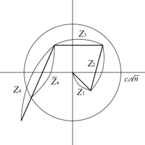
Figure 2: An example of the random variables $N(n)\,(=4)$, $Z_{i}$ and $\bar{Z}_{N(n)}$.

Lemma 5

$\text{E}[N(n)]$ scales as $\Theta(n^{\frac{\alpha}{2}})$ for $\alpha\in(0,2]$.

Proof: From Lemma 3, we have $\lim_{n\to\infty}\text{P}\{T_{\text{LF}}(c_{d}\sqrt{n})\leq\hat{t}(n)\}=1$ when $\hat{t}(n)=\Theta(n^{\frac{\alpha}{2}+\hat{\epsilon}})$ for $\alpha\in(0,2]$ and an arbitrary $\hat{\epsilon}>0$. Hence, we have

$$\text{E}[T_{\text{LF}}(c_{d}\sqrt{n})]=O(n^{\frac{\alpha}{2}+\hat{\epsilon}}).$$ (26)

From Lemma 4, we have $\lim_{n\to\infty}\text{P}\{T_{\text{LF}}(c_{d}\sqrt{n})>\tilde{t}(n)\}=1$ when $\tilde{t}(n)=\Theta(n^{\frac{\alpha}{2}-\tilde{\epsilon}})$ for $\alpha\in(0,2]$ and an arbitrary $\tilde{\epsilon}>0$. Thus, we have

$$\text{E}[T_{\text{LF}}(c_{d}\sqrt{n})]=\Omega(n^{\frac{\alpha}{2}-\tilde{\epsilon}}).$$ (27)

By choosing $\hat{\epsilon}$ and $\tilde{\epsilon}$ arbitrarily small, from (26) and (27), we have

$$\text{E}[T_{\text{LF}}(c_{d}\sqrt{n})]=\Theta(n^{\frac{\alpha}{2}})\quad\forall\alpha\in(0,2].$$ (28)

Note from (25) that

$$\text{E}[T_{\text{LF}}(c_{d}\sqrt{n})]\leq\text{E}[N(n)]\leq\text{E}[T_{\text{LF}}(c_{d}\sqrt{n})]+1,$$ (29)

which shows that the order of $\text{E}[N(n)]$ is the same as that of $\text{E}[T_{\text{LF}}(c_{d}\sqrt{n})]$. Therefore, combining (28) and (29) yields the lemma. $\square$

With the help of Lemma 5, we can derive an upper bound for the critical delay under Lévy walk.

Lemma 6 (Upper bound for Lévy walk)

Suppose that under Lévy walk with a distribution parameter $\alpha$, the time $t\triangleq\hat{t}(n)$ in $\text{P}\{T(c_{d}\sqrt{n})>t\}$ scales as $\Theta(n^{\frac{1}{2}+\epsilon_{1}})$ for an arbitrary $\epsilon_{1}>0$ and $\alpha\in(0,1)$, and $\Theta(n^{\frac{\alpha}{2}+\epsilon_{2}})$ for an arbitrary $\epsilon_{2}>0$ and $\alpha\in[1,2]$. Then, we have

$$\lim_{n\to\infty}\text{P}\{T(c_{d}\sqrt{n})>\hat{t}(n)\}=0,$$

which shows that the critical delay $C_{\Pi}(n)$ under Lévy walk scales as $O(n^{\frac{1}{2}})$ for $\alpha\in(0,1)$ and $O(n^{\frac{\alpha}{2}})$ for $\alpha\in[1,2]$.

Proof: Using Markov’s inequality [29], we have

$$\text{P}\{T(c_{d}\sqrt{n})>\hat{t}(n)\}\leq\frac{\text{E}[T(c_{d}\sqrt{n})]}{\hat{t}(n)}.$$ (30)

We calculate the expectation $\text{E}[T(c_{d}\sqrt{n})]$ on the right-hand side of (30) by conditioning on the values of $N(n)$ as

$$\text{E}[T(c_{d}\sqrt{n})] =\text{E}\!\left[\text{E}[T(c_{d}\sqrt{n})\,|\,N(n)]\right]$$

$$=\sum_{k=1}^{\infty}\text{E}[T(c_{d}\sqrt{n})\,|\,N(n)=k]\cdot\text{P}\{N(n)=k\}.$$ (31)

From (23), we have for $k=1$,

$$\text{E}[T(c_{d}\sqrt{n})\,|\,N(n)=k] =c_{d}\sqrt{n}.$$ (32)

In addition, from (23), we have for $k=2,3,\ldots$,

$$\text{E}[T(c_{d}\sqrt{n})\,|\,N(n)=k]$$

$$=\text{E}\left[\sum_{i=1}^{N(n)-1}Z_{i}+\bar{Z}_{N(n)}\,\bigg{|}\,N(n)=k\right]$$

$$=\sum_{i=1}^{k-1}\text{E}[Z_{i}\,|\,N(n)=k]+\text{E}[\bar{Z}_{k}\,|\,N(n)=k].$$ (33)

The random variables $Z_{i}\,(i=1,\ldots,k-1)$ and $\bar{Z}_{k}$ in (6) are correlated with the random variable $N(n)\,(=k)$, whereas the random variables $Z_{i}\,(i=k+1,k+2,\ldots)$ are independent of $N(n)\,(=k)$. Specifically, for $i=1,\ldots,k-1$, the step size $Z_{i}$ should be less than the diameter of the disc $\mathcal{D}(n)$ (i.e., $2c_{d}\sqrt{n}$). In addition, the truncated step size $\bar{Z}_{k}$ should satisfy the inequality in (24). Hence, the conditional expectations on the right-hand side of (6) are bounded as follows:

$$\begin{split}&\text{E}[Z_{i}|N(n)=k]\leq\text{E}[Z|Z\leq 2c_{d}\sqrt{n}],\\ &\text{E}[\bar{Z}_{k}|N(n)=k]\leq 2c_{d}\sqrt{n},\end{split}$$ (34)

where $Z$ denotes the generic random variable for $Z_{i}$. Combining (6)-(34), we obtain an upper bound for $\text{E}[T(c_{d}\sqrt{n})]$ as follows:

$$\text{E}[T(c_{d}\sqrt{n})]$$

$$\leq c_{d}\sqrt{n}\cdot\text{P}\{N(n)=1\}+2c_{d}\sqrt{n}\sum_{k=2}^{\infty}\text{P}\{N(n)=k\}$$

$$\quad+\text{E}[Z|Z\leq 2c_{d}\sqrt{n}]\sum_{k=2}^{\infty}(k-1)\cdot\text{P}\{N(n)=k\}$$

$$\leq 2c_{d}\sqrt{n}\sum_{k=1}^{\infty}\text{P}\{N(n)=k\}$$

$$\quad+\text{E}[Z|Z\leq 2c_{d}\sqrt{n}]\sum_{k=1}^{\infty}k\cdot\text{P}\{N(n)=k\}$$

$$=2c_{d}\sqrt{n}+\text{E}[Z|Z\leq 2c_{d}\sqrt{n}]\cdot\text{E}[N(n)].$$ (35)

Using (3), we can calculate the conditional expectation $\text{E}[Z|Z\leq 2c_{d}\sqrt{n}]$ in (6) and it scales for each $\alpha\in(0,2]$ as follows:

$$\text{E}[Z|Z\leq 2c_{d}\sqrt{n}]$$

$$=\begin{cases}\frac{\alpha}{1-\alpha}\frac{(2c_{d}\sqrt{n})^{1-\alpha}-1}{1-(2c_{d}\sqrt{n})^{-\alpha}}&\text{ for }\alpha\in(0,1),\\ \frac{\log(2c_{d}\sqrt{n})}{1-(2c_{d}\sqrt{n})^{-1}}&\text{ for }\alpha=1,\\ \frac{\alpha}{\alpha-1}\frac{1-(2c_{d}\sqrt{n})^{1-\alpha}}{1-(2c_{d}\sqrt{n})^{-\alpha}}&\text{ for }\alpha\in(1,2),\\ \frac{\sqrt{2}\sigma}{\sqrt{\pi}}\frac{\exp(-1/2\sigma^{2})-\exp(-2(c_{d})^{2}n/\sigma^{2})}{\mathrm{erf}(c_{d}\sqrt{2n}/\sigma)-\mathrm{erf}(1/\sqrt{2}\sigma)}&\text{ for }\alpha=2,\\ \end{cases}$$

$$=\begin{cases}\Theta(n^{(1-\alpha)/2})&\text{ for }\alpha\in(0,1),\\ \Theta(\log(n))&\text{ for }\alpha=1,\\ \Theta(n^{0})&\text{ for }\alpha\in(1,2].\end{cases}$$

Since $\text{E}[N(n)]$ scales as $\Theta(n^{\frac{\alpha}{2}})$ by Lemma 5, the term on the right-hand side of (6) scales as

$$2c_{d}\sqrt{n}+\text{E}[Z|Z\leq 2c_{d}\sqrt{n}]\cdot\text{E}[N(n)]$$

$$=\begin{cases}\Theta(n^{\frac{1}{2}})&\text{ for }\alpha\in(0,1),\\ \Theta(n^{\frac{1}{2}}\log(n))&\text{ for }\alpha=1,\\ \Theta(n^{\frac{\alpha}{2}})&\text{ for }\alpha\in(1,2].\end{cases}$$ (36)

Thus, we have from (6) and (6) the following:

$$\lim_{n\to\infty}\frac{\text{E}[T(c_{d}\sqrt{n})]}{\hat{t}(n)}$$

$$\leq\lim_{n\to\infty}\frac{2c_{d}\sqrt{n}+\text{E}[Z|Z\leq 2c_{d}\sqrt{n}]\cdot\text{E}[N(n)]}{\hat{t}(n)}$$

$$=0.$$

Therefore, from (30), we have

$$\lim_{n\to\infty}\text{P}\{T(c_{d}\sqrt{n})>\hat{t}(n)\}\leq\lim_{n\to\infty}\frac{\text{E}[T(c_{d}\sqrt{n})]}{\hat{t}(n)}\leq 0,$$

i.e., $\lim_{n\to\infty}\text{P}\{T(c_{d}\sqrt{n})>\hat{t}(n)\}=0$. This completes the proof. $\square$

Lemma 7 (Lower bound for Lévy walk)

Suppose that under Lévy walk with a distribution parameter $\alpha$, the time $t\triangleq\tilde{t}(n)$ in $\text{P}\{T(c_{d}\sqrt{n})>t\}$ scales as $\Theta(n^{\frac{1}{2}-\epsilon_{1}})$ for an arbitrary $\epsilon_{1}>0$ and $\alpha\in(0,1)$, and $\Theta(n^{\frac{\alpha}{2}-\epsilon_{2}})$ for an arbitrary $\epsilon_{2}>0$ and $\alpha\in(1,2]$. Then, we have

$$\lim_{n\to\infty}\text{P}\{T(c_{d}\sqrt{n})>\tilde{t}(n)\}=1,$$

which shows that the critical delay $C_{\Pi}(n)$ under Lévy walk scales as $\Omega(n^{\frac{1}{2}})$ for $\alpha\in(0,1)$ and $\Omega(n^{\frac{\alpha}{2}})$ for $\alpha\in[1,2]$.

Proof: We will prove this lemma by showing for each of the cases of $\alpha\in(0,1)$ and $\alpha\in[1,2]$ that

$$\lim_{n\to\infty}\text{P}\{T(c_{d}\sqrt{n})\leq\tilde{t}(n)\}=0.$$

We first consider the case of $\alpha\in(0,1)$. Since a Lévy walker moves with a constant velocity $v=1$, it takes at least $c_{d}\sqrt{n}$ time to exit from the disc $\mathcal{D}(n)$. Thus, it is obvious that

$$\text{P}\{T(c_{d}\sqrt{n})<c_{d}\sqrt{n}\}=0.$$ (37)

Since $\tilde{t}(n)=\Theta(n^{\frac{1}{2}-\epsilon_{1}})$, there exists a constant $\tilde{n}\in\mathbb{N}$ such that $\tilde{t}(n)<c_{d}\sqrt{n}$ for $n\geq\tilde{n}$. Hence, we have for $n\geq\tilde{n}$

$$\text{P}\{T(c_{d}\sqrt{n})\leq\tilde{t}(n)\} \leq\text{P}\{T(c_{d}\sqrt{n})<c_{d}\sqrt{n}\}.$$ (38)

Combining (37) and (38) and then taking limits, we have

$$\lim_{n\to\infty}\text{P}\{T(c_{d}\sqrt{n})\leq\tilde{t}(n)\} \leq\lim_{n\to\infty}\text{P}\{T(c_{d}\sqrt{n})<c_{d}\sqrt{n}\}$$

$$=0,$$

i.e., $\lim_{n\to\infty}\text{P}\{T(c_{d}\sqrt{n})\leq\tilde{t}(n)\}=0$. We have proved the lemma in the case of $\alpha\in(0,1)$.

We next consider the case of $\alpha\in[1,2]$. In the following, we use the notations $T_{\text{LF}}(\cdot)$ and $T_{\text{LW}}(\cdot)$ to distinguish the first exit times between Lévy flight and Lévy walk. We will show based on (23) and (25) that for $t\geq 0$,

$$\text{P}\{T_{\text{LW}}(c_{d}\sqrt{n})\leq t\}\leq\text{P}\{T_{\text{LF}}(c_{d}\sqrt{n})\leq t+1\}.$$ (39)

From (23), if $N(n)=1$, then $T_{\text{LW}}(c_{d}\sqrt{n})=c_{d}\sqrt{n}>0=N(n)-1.$ In addition, if $N(n)\geq 2$, then $T_{\text{LW}}(c_{d}\sqrt{n})=\sum_{i=1}^{N(n)-1}Z_{i}+\hat{Z}_{N}>\sum_{i=1}^{N(n)-1}Z_{i}\geq N(n)-1,$ where the last inequality comes from the assumption that the step size $Z$ has a lower bound at 1 (given in Section IV). Combining above two cases gives

$$T_{\text{LW}}(c_{d}\sqrt{n})\geq N(n)-1.$$

From (25), we obtain $N(n)\stackrel{{\scriptstyle\text{d}}}{{=}}\lceil T_{\text{LF}}(c_{d}\sqrt{n})\rceil\geq T_{\text{LF}}(c_{d}\sqrt{n})$. Thus, we have with probability 1,

$$T_{\text{LW}}(c_{d}\sqrt{n})\geq T_{\text{LF}}(c_{d}\sqrt{n})-1.$$

This proves (39). Substituting $t=\tilde{t}(n)$ into (39), we obtain

$$\text{P}\{T_{\text{LW}}(c_{d}\sqrt{n})\leq\tilde{t}(n)\}\leq\text{P}\{T_{\text{LF}}(c_{d}\sqrt{n})\leq\tilde{t}(n)\!+\!1\}.$$ (40)

For $\tilde{t}(n)$ scaling as $\Theta(n^{\frac{\alpha}{2}-\epsilon_{2}})$, $\tilde{t}(n)+1$ also scales as $\Theta(n^{\frac{\alpha}{2}-\epsilon_{2}})$. Consequently, by Lemma 4, the probability on the right-hand side of (40) becomes in the limit:

$$\lim_{n\to\infty}\text{P}\{T_{\text{LF}}(c_{d}\sqrt{n})\leq\tilde{t}(n)+1\}=0.$$

Therefore, from (40), we have $\lim_{n\to\infty}\text{P}\{T_{\text{LW}}(c_{d}\sqrt{n})\leq\tilde{t}(n)\}=0$, which proves the lemma in the case of $\alpha\in[1,2]$. This completes the proof. $\square$

Combining Lemmas 6 and 7 yields the following theorem.

Theorem 2

The critical delay $\bm{C_{\Pi}\text{\bf{(}}n\text{\bf{)}}}$ under Lévy walk with a distribution parameter $\alpha$ scales as $\bm{\Theta\text{\bf(}n^{\frac{1}{2}}\text{\bf)}}$ for $\alpha\in(0,1)$ and $\bm{\Theta\text{\bf{(}}n^{\frac{\text{\boldmath{$\alpha$}\unboldmath}}{2}}\text{\bf)}}$ for $\alpha\in[1,2].$

VII Discussion

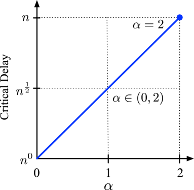
(a) Lévy flight

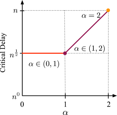
(b) Lévy walk

Figure 3: Critical delays under Lévy flight and Lévy walk for different $\alpha.$

We summarize the high-level interpretations of this paper. Fig. 3. shows the critical delays under Lévy walk and Lévy flight, parameterized by $\alpha.$ Lévy flight shows that the critical delay proportionally increases with $\alpha.$ However, in the case of the Lévy walk, we can find a phase transition such that when $\alpha\in(0,1),$ the critical delay is constantly $\Theta(n^{\frac{1}{2}})$ and shifts to the proportional increasing phase when $\alpha\in[1,2].$ Two different scaling regions are essentially related to the fact that the mean step size of Lévy walk for $\alpha\in(0,1)$ is infinite but finite for $\alpha\in[1,2].$ In contrast to Lévy walk, the travel time independence of step size in Lévy flight leads to continuous scaling over $\alpha$. Note that for $\alpha=2$ (i.e., Brownian motion) our result coincides with that in [6] which also studied the critical delay under Brownian motion.

By using values of $\alpha$ from experimental measurements from [7], we can see how network delay scales with human mobility in practice. To give an insight to the readers, we show $\alpha$ values measured from five different sites in Table I presented in [7] with a flight extraction method, “rectangle”. We see that critical delays for human mobility range from $\Theta(n^{0.27})$ to $\Theta(n^{0.91})$. Human mobility mainly has $\alpha>1$, in which case a longer delay than $\Theta(\sqrt{n})$ is needed. This implies that it may be hard to design a low delay protocol for mobile networks under human mobility.

TABLE I: Experimental $\alpha$ values for different sites presented in [7].

Site	$\alpha$	Site	$\alpha$
KAIST	0.53	New York City	1.62
NCSU	1.27	Disney World	1.20
		State fair	1.81

Our contribution is not restricted to the mathematical derivation of delay scaling for new mobility models. We provided techniques that connect the diffusion equation of a continuous time random walk to the delay scaling as well as that analyze the delay scaling of semi-Markovian movements. We expect that our techniques can be further developed to the analysis of other detailed performance metrics such as contact time distribution and the generalized delay-capacity tradeoff for various levels of per-node throughput.

Future work includes investigation of throughput and delay scaling for mobile networks with heterogeneous and collective node mobilities. In addition to the recent research topics on “per-node throughput scaling” under inhomogeneous spatial node distributions (i.e., Cox process, Neyman-Scott process, Matérn cluster process and Thomas process), e.g., [30, 31], our paper can be an important step to the study of delay scaling under such heterogeneous networks. There is an insight from [8] that in human-assisted networks, the actual delays might be even shorter. This is because human mobility is not completely random: people tend to visit the same locations and regularly meet a group of people every day. Although their mobility can be characterized by heavy-tail distributions, these regularity in daily mobility significantly facilitates routing of packets among people (as long as they are socially connected). Therefore, there remains a possibility of designing a low delay protocol for mobile networks under heterogeneous human mobility by judiciously utilizing these social factors.

VIII Conclusion

We have presented Lévy mobility models consisting of Lévy flight and Lévy walk parameterized by $\alpha$ and studied the critical delay under both mobility models. Lévy mobility is known as a realistic human mobility so that the critical delay we provided here can be essential in designing an architecture and protocols of a wireless mobile network. The insight that the critical delay scales as $\Theta(n^{\frac{\alpha}{2}})$ for Lévy mobility models in the range of $\alpha\in[1,2]$ is especially important because it is anticipating that the delay of mobile networks with human mobility (e.g., smartphone networks, pocket switched networks) could be quite high in practice, considering the $\alpha$ values measured in real traces. The insight tells that mobile networks operated by human mobility patterns may need to prepare an alternative path for delay sensitive data as well as even for delay tolerable data whose tolerance level is limited.

Appendix A Critical Delay Analysis for Lévy Flight without Continuous Limit

In Section V, we have studied the critical delay under Lévy flight using continuous limit. By following the technique in [6], we can study the critical delay without continuous limit (i.e., with a non-zero scale factor $|c|$) and can derive a lower bound for the critical delay under Lévy flight. Lemma 8 summarizes the result.

Lemma 8

With a non-zero scale factor $|c|$, the critical delay $C_{\Pi}(n)$ under Lévy flight with a distribution parameter $\alpha\in(0,2]$ scales as $\Omega(n^{\frac{\alpha}{2}})$.

Before proving the lemma, we give a remark. The scaling property of the critical delay with continuous limit (shown in Theorem 1) works as an upper bound for the one without continuous limit. Hence, the result in Lemma 8 shows that our analysis in Section V gives the tightest upper bound, which justifies our technique using continuous limit. We now give the proof of Lemma 8.

Proof: Similarly to the proof of Lemma 4, we will prove this lemma by showing that

$$\lim_{n\to\infty}\text{P}\{T_{x}(c_{d}\sqrt{n}/\sqrt{2})\leq\tilde{t}(n)\}=0,$$ (41)

where $\tilde{t}(n)=\Theta(n^{\frac{\alpha}{2}-\epsilon})$ for an arbitrary $\epsilon>0$ and $\alpha\in(0,2]$. Then, from (6), we obtain $\lim_{n\to\infty}\text{P}\{T(c_{d}\sqrt{n})\leq\tilde{t}(n)\}\leq 2\lim_{n\to\infty}\text{P}\{T_{x}(c_{d}\sqrt{n}/\sqrt{2})\leq\tilde{t}(n)\}=0$. That is, we have $\lim_{n\to\infty}\text{P}\{T(c_{d}\sqrt{n})\leq\tilde{t}(n)\}=0$, or equivalently, $\lim_{n\to\infty}\text{P}\{T(c_{d}\sqrt{n})>\tilde{t}(n)\}=1$, which shows that the critical delay $C_{\Pi}(n)$ scales as $\Omega(n^{\frac{\alpha}{2}})$.

Without loss of generality, we assume $\mathbf{X}(0)=(0,0)$. Then, from (2), $X_{x}(t)$ for $t=1,2,\ldots$ can be expressed as

$$X_{x}(t)=\sum_{i=1}^{t}Z_{i}\cos\theta_{i}.$$ (42)

Let $Z\cos\theta$ denote the generic random variable for $Z_{i}\cos\theta_{i}$. By the independence of random variables $Z$ and $\theta$, the mean of $Z\cos\theta$ is given by $\text{E}[Z\cos\theta]=\text{E}[Z]\text{E}[\cos\theta]=0$. Hence, from (42), the mean of $X_{x}(t)$ is given by $\text{E}[X_{x}(t)]=t\text{E}[Z\cos\theta]=0$ and the variance of $X_{x}(t)$ becomes $\text{E}[(X_{x}(t))^{2}]=t\text{E}[(Z\cos\theta)^{2}]$. Thus, Hoeffding’s inequality [6] gives an upper bound for $\text{P}\{X_{x}(t)\geq r/\sqrt{2}\}$ as follows: $\text{P}\{X_{x}(t)\geq r/\sqrt{2}\}\leq\exp\left(-\frac{r^{2}}{8t\text{E}[(Z\cos\theta)^{2}]}\right).$ By the symmetry of node motion, we have

$$\text{P}\{|X_{x}(t)|\geq r/\sqrt{2}\} \leq 2\exp\left(-\frac{r^{2}}{8t\text{E}[(Z\cos\theta)^{2}]}\right).$$ (43)

Due to (A1), the event $\{T_{x}(r/\sqrt{2})\leq k\}$ for $k=1,2,\ldots$ implies the event $\bigcup_{t=1}^{k}\{|X_{x}(t)|\geq r/\sqrt{2}\}$. Hence, we have

$$\text{P}\{T_{x}(r/\sqrt{2})\leq k\} \leq\sum_{t=1}^{k}\text{P}\{|X_{x}(t)|\geq r/\sqrt{2}\}$$

$$\leq 2\sum_{t=1}^{k}\exp\left(-\frac{r^{2}}{8t\text{E}[(Z\cos\theta)^{2}]}\right)$$

$$\leq 2k\exp\left(-\frac{r^{2}}{8k\text{E}[(Z\cos\theta)^{2}]}\right),$$ (44)

where the second inequality comes from (43). Substituting $r=c_{d}\sqrt{n}$ and $k=\tilde{t}(n)$ into (A), we have

$$\begin{split}\@ADDCLASS{ltx_eqn_lefteqn}$\displaystyle\text{P}\{T_{x}(c_{d}\sqrt{n}/\sqrt{2})\leq\tilde{t}(n)\}$\mbox{}\hfil\\ &\quad\leq 2\tilde{t}(n)\exp\left(-\frac{(c_{d})^{2}n}{8\tilde{t}(n)\text{E}[(Z\cos\theta)^{2}]}\right).\end{split}$$ (45)

In the following, we will derive a bound for $\text{E}[(Z\cos\theta)^{2}]$. Since $\text{E}[(Z\cos\theta)^{2}]=\text{E}[(Z|\cos\theta|)^{2}]$, we have

$$\text{E}[(Z\cos\theta)^{2}] =\int_{0}^{\sqrt{n}}z^{2}\text{d}F_{Z|\cos\theta|}(z).$$ (46)

We first consider the case of $\alpha\in(0,2)$. From the CCDF of $Z|\cos\theta|$ given for $z\geq 1$ in (12), we have for $z\geq 1$,

$$\frac{\text{d}F_{Z|\cos\theta|}(z)}{\text{d}z} =-\frac{\text{d}}{\text{d}z}\text{P}\{Z|\cos\theta|>z\}$$

$$=\frac{2\alpha c(n)}{\pi z^{\alpha+1}}\int_{0}^{\cos^{-1}(\frac{z}{\sqrt{n}})}(\cos\vartheta)^{\alpha}\text{d}\vartheta$$

$$\leq\frac{\alpha c^{\star}c(n)}{z^{\alpha+1}}.$$

Thus, the integral on the right-hand side of (46) is bounded above by

$$\int_{0}^{\sqrt{n}}z^{2}\text{d}F_{Z|\cos\theta|}(z)$$

$$=\int_{0}^{1}z^{2}\text{d}F_{Z|\cos\theta|}(z)+\int_{1}^{\sqrt{n}}z^{2}\text{d}F_{Z|\cos\theta|}(z)$$

$$\leq\text{P}\{0\leq Z|\cos\theta|\leq 1\}+\int_{1}^{\sqrt{n}}z^{2}\frac{\alpha c^{\star}c(n)}{z^{\alpha+1}}\text{d}z$$

$$=\text{P}\{0\leq Z|\cos\theta|\leq 1\}+\frac{\alpha c^{\star}c(n)}{2-\alpha}(n^{1-\frac{\alpha}{2}}-1),$$

from which we have

$$\text{E}[(Z\cos\theta)^{2}]=O(n^{1-\frac{\alpha}{2}})\quad\text{ for }\alpha\in(0,2).$$ (47)

We next consider the case of $\alpha=2$. By following the approach in the case of $\alpha\in(0,2)$, we have

$$\text{E}[(Z\cos\theta)^{2}]=O(n^{1-\frac{\alpha}{2}})\quad\text{ for }\alpha=2.$$ (48)

Combining (47) and (48) gives $\text{E}[(Z\cos\theta)^{2}]=O(n^{1-\frac{\alpha}{2}})$ for $\alpha\in(0,2]$. Hence, there exist constants $\bar{n}\in\mathbb{N}$ and $\bar{c}>0$ such that

$$\text{E}[(Z\cos\theta)^{2}]\leq\bar{c}n^{1-\frac{\alpha}{2}}\quad\text{ for all }n\geq\bar{n}.$$ (49)

In addition, since $\tilde{t}(n)=\Theta(n^{\frac{\alpha}{2}-\epsilon})$, there exist constants $\tilde{n}\in\mathbb{N}$ and $\tilde{c}>0$ such that

$$\tilde{t}(n)\leq\tilde{c}n^{\frac{\alpha}{2}-\epsilon}\quad\text{ for all }n\geq\tilde{n}.$$ (50)

By (49) and (50), the term on the right-hand side of (45) is further bounded by

$$\begin{split}\@ADDCLASS{ltx_eqn_lefteqn}$\displaystyle 2\tilde{t}(n)\exp\left(-\frac{(c_{d})^{2}n}{8\tilde{t}(n)\text{E}[(Z\cos\theta)^{2}]}\right)$\mbox{}\hfil\\ &\quad\leq 2\tilde{c}n^{\frac{\alpha}{2}-\epsilon}\exp\left(-\frac{(c_{d})^{2}n^{\epsilon}}{8\tilde{c}\bar{c}}\right).\end{split}$$ (51)

By L’Hôspital’s rule, (51) becomes in the limit as

$$\begin{split}\@ADDCLASS{ltx_eqn_lefteqn}$\displaystyle\lim_{n\to\infty}2\tilde{t}(n)\exp\left(-\frac{(c_{d})^{2}n}{8\tilde{t}(n)\text{E}[(Z\cos\theta)^{2}]}\right)$\mbox{}\hfil\\ &\quad\leq\lim_{n\to\infty}2\tilde{c}n^{\frac{\alpha}{2}-\epsilon}\exp\left(-\frac{(c_{d})^{2}n^{\epsilon}}{8\tilde{c}\bar{c}}\right)=0.\end{split}$$ (52)

Combining (45) and (52) proves (41). This completes the proof. $\square$

Kyunghan Lee (S’07-M’10) received his B.S., M.S. and Ph.D. degrees from Electrical Engineering and Computer Science from Korea Advanced Institute of Science and Technology (KAIST), Daejeon, Korea in 2002, 2004 and 2009, respectively. He is currently a Senior Research Scholar in the Department of Computer Science at North Carolina State University. His research interests are in the areas of human mobility, delay tolerant networks, context-aware services and applications, mobile system and protocol design.

Yoora Kim (S’05-M’09) received her B.S., M.S. and Ph.D. degrees in Mechanical Engineering, Applied Mathematics and Mathematical Sciences from Korea Advanced Institute of Science and Technology (KAIST), Daejeon, Korea, in 2003, 2005 and 2009, respectively. She is currently a post-doctoral research associate at The Ohio State University. Her research interests include modeling, design, and performance evaluation of communication systems, and scheduling and resource allocation problems in wireless networks under various stochastic dynamics.

Song Chong (M’93) received the B.S. and M.S. degrees in Control and Instrumentation Engineering from Seoul National University, Seoul, Korea, in 1988 and 1990, respectively, and the Ph.D. degree in Electrical and Computer Engineering from the University of Texas at Austin in 1995. Since March 2000, he has been with the Department of Electrical Engineering, Korea Advanced Institute of Science and Technology (KAIST), Daejeon, Korea, where he is a Professor and was the Head of the Communications and Computing Group of the department. Prior to joining KAIST, he was with the Performance Analysis Department, AT&T Bell Laboratories, New Jersey, as a Member of Technical Staff. His current research interests include wireless networks, future Internet, and human mobility characterization and its applications to mobile networking. He has published more than 100 papers in international journals and conferences. He is an Editor of Computer Communications journal and Journal of Communications and Networks. He has served on the Technical Program Committee of a number of leading international conferences including IEEE INFOCOM and ACM CoNEXT. He serves on the Steering Committee of WiOpt and was the General Chair of WiOpt’09. He is currently the Chair of Wireless Working Group of the Future Internet Forum of Korea and the Vice President of the Information and Communication Society of Korea.

Injong Rhee (S’89-M’94) received his Ph.D. from the University of North Carolina at Chapel Hill. He is a Professor in the Department of Computer Science at North Carolina State University. He is an Editor of IEEE Transactions on Mobile Computing. His areas of research interests include computer networks, congestion control, wireless ad hoc networks and sensor networks.

Yung Yi (S’04-M’06) received his B.S. and the M.S. in the School of Computer Science and Engineering from Seoul National University, South Korea in 1997 and 1999, respectively, and his Ph.D. in the Department of Electrical and Computer Engineering at the University of Texas at Austin in 2006. From 2006 to 2008, he was a post-doctoral research associate in the Department of Electrical Engineering at Princeton University. Now, he is an associate professor at the Department of Electrical Engineering at KAIST, South Korea. He has been serving as a TPC member at various conferences including ACM Mobihoc, Wicon, WiOpt, IEEE Infocom, ICC, Globecom, and ITC. His academic service also includes the local arrangement chair of WiOpt 2009 and CFI 2010, the networking area track chair of TENCON 2010, and the publication chair of CFI 2010, and a guest editor of the special issue on Green Networking and Communication Systems of IEEE Surveys and Tutorials. He also serves as the co-chair of the Green Multimedia Communication Interest Group of the IEEE Multimedia Communication Technical Committee. His current research interests include the design and analysis of computer networking and wireless systems, especially congestion control, scheduling, and interference management, with applications in wireless ad hoc networks, broadband access networks, economic aspects of communication networks economics, and greening of network systems.

Ness B. Shroff (S’91-M’93-SM’01-F’07) received the Ph.D. degree from Columbia University, New York, NY, in 1994. He currently holds the Ohio Eminent Scholar chaired professorship in Networking and Communications in the departments of ECE and CSE at The Ohio State University, in Columbus, OH. He also currently serves as a Guest Chaired Professor of wireless communications with the Department of Electronic Engineering, Tsighnua University, Beijing, China. Previously, he was a Professor of ECE with Purdue University, West Lafayette, IN, and the Director of the Center for Wireless Systems and Applications (CWSA), a university-wide center on wireless systems and applications. His research interests span the areas of communications, social, and cyber-physical networks, where he investigates fundamental problems in the design, performance, pricing, and security of these networks. Dr. Shroff has received numerous awards for his networking research, including the National Science Foundation CAREER award, the Best Paper awards for IEEE INFOCOM 2006 and 2008, the Best Paper Award for IEEE IWQoS 2006, the Best Paper of the Year Award for Computer Networks, and the Best Paper of the Year Award for the Journal of Communications and Networks (his IEEE INFOCOM 2005 paper was one of two runner-up papers).

References

- [1] P. Gupta and P. R. Kumar, “The capacity of wireless networks,” IEEE Transaction on Information Theory, vol. 46, no. 2, pp. 388–404, 2000.
- [2] M. Grossglauser and D. N. C. Tse, “Mobility increases the capacity of ad hoc wireless networks,” IEEE/ACM Transactions on Networking, vol. 10, no. 4, pp. 477–486, 2002.
- [3] S. Toumpis and A. Goldsmith, “Large wireless networks under fading, mobility, and delay constraints,” in Proceedings of IEEE INFOCOM, 2004.
- [4] M. Neely and E. Modiano, “Capacity and delay tradeoffs for ad-hoc mobile networks,” IEEE Transaction on Information Theory, vol. 51, no. 6, pp. 1917–1937, 2005.
- [5] X. Lin, G. Sharma, R. R. Mazumdar, and N. B. Shroff, “Degenerate delay-capacity tradeoffs in ad-hoc networks with brownian mobility,” IEEE/ACM Transactions on Networking, vol. 14, pp. 2777–2784, 2006.
- [6] G. Sharma, R. Mazumdar, and N. B. Shroff, “Delay and capacity trade-offs in mobile ad hoc networks: a global perspective,” IEEE/ACM Transactions on Networking, vol. 15, no. 5, pp. 981–992, 2007.
- [7] I. Rhee, M. Shin, S. Hong, K. Lee, and S. Chong, “On the levy walk nature of human mobility,” in Proceedings of INFOCOM, 2008.
- [8] K. Lee, S. Hong, S. Kim, I. Rhee, and S. Chong, “Slaw: A new human mobility model,” in Proceedings of IEEE INFOCOM, 2009.
- [9] M. C. Gonzalez, C. A. Hidalgo, and A.-L. Barabasi, “Understanding individual human mobility patterns,” Nature, vol. 453, pp. 779–782, June 2008.
- [10] M. F. Shlesinger, G. M. Zaslavsky, and J. Klafter, “Levy dynamics of enhanced diffusion: Application to turbulence,” Physical Review Letters, vol. 58, pp. 1100–1103, March 1987.
- [11] M. Franceschetti, O. Dousse, D. Tse, and P. Thiran, “Closing the gap in the capacity of wireless networks via percolation theory,” IEEE Transactions on Information Theory, vol. 53, no. 3, pp. 1009–1018, 2007.
- [12] A. Agarwal and P. R. Kumar, “Capacity bounds for ad hoc and hybrid wireless networks,” ACM SIGCOMM Computer Communication Review, vol. 34, no. 3, pp. 71–81, 2004.
- [13] N. Bansal and Z. Liu, “Capacity, delay and mobility in wireless ad-hoc networks,” in Proceedings of IEEE INFOCOM, 2003.
- [14] E. Perevalov and R. Blum, “Delay limited capacity of ad hoc networks: Asymptotically optimal transmission and relaying strategy,” in Proceedings of IEEE INFOCOM, 2003.
- [15] A. Tsirigos and Z. J. Haas, “Multipath routing in the presence of frequent topological changes,” IEEE Communication Magazine, vol. 39, no. 11, pp. 132–138, 2001.
- [16] G. Sharma and R. Mazumdar, “Scaling laws for capacity and delay in wireless ad hoc networks with random mobility,” in Proceedings of IEEE ICC, 2004.
- [17] X. Lin and N. B. Shroff, “The fundamental capacity-delay tradeoff in large mobile ad hoc networks,” in Proceedings of 3rd Annual Mediterranean Ad Hoc Networking Workshop, 2004.
- [18] M. Neely and E. Modiano, “Dynamic power allocation and routing for satellite and wireless networks with time varying channels,” in Ph.D Thesis, Massachusetts Institute of Technology, 2004.
- [19] A. El Gamal, J. Mammen, B. Prabhakar, and D. Shah, “Optimal throughput-delay scaling in wireless networks: Part I: the fluid model,” IEEE/ACM Transactions on Networking, vol. 14, pp. 2568–2592, 2006.
- [20] P. M. Drysdale and P. A. Robinson, “Lévy random walks in finite systems,” Physical Review E, vol. 58, no. 5, pp. 5382–5394, 1998.
- [21] R. Metzler and J. Klafter, “The random walk’s guide to anomalous diffusion: A fractional dynamics approach,” Physics Reports, vol. 339, no. 1, pp. 1–77, 2000.
- [22] A. V. Chechkin, V. Y. Gonchar, J. Klafter, and R. Metzler, “Fundamentals of lévy flight processes,” Advances in Chemical Physics, vol. 133, pp. 439–496, 2006.
- [23] J. P. Nolan, Stable Distributions - Models for Heavy Tailed Data. Boston: Birkhauser, 2012, in progress, Chapter 1 online at academic2.american.edu/jpnolan.
- [24] M. Ferraro and L. Zaninetti, “Mean number of visits to sites in levy flights,” Physical Review E, vol. 73, May 2006.
- [25] S. Redner, A Guide to First-passage Processes. New York: Cambridge University Press, 2001.
- [26] M. Gitterman, “Mean first passage time for anomalous diffusion,” Physical Review E, vol. 62, no. 5, pp. 6065–6070, 2000.
- [27] I. Podlubny, Fractional Differential Equations. London: Academic Press, 1999.
- [28] J. E. Marsden and M. J. Hoffman, Elementary Classical Analysis. New York: W. H. Freeman and Company, 1993.
- [29] S. M. Ross, Stochastic Processes. New York: John Wiley & Sons, 1996.
- [30] M. Garetto, P. Giaccone, and E. Leonardi, “Capacity scaling in ad hoc networks with heterogeneous mobile nodes: the super-critical regime,” IEEE/ACM Transactions on Networking, vol. 17, no. 5, pp. 1522–1535, 2009.
- [31] G. Alfano, M. Garetto, E. Leonardi, and V. Martina, “Capacity scaling of wireless networks with inhomogeneous node density: Lower bounds,” IEEE/ACM Transactions on Networking, vol. 18, no. 5, pp. 1624–1636, 2010.