Coupled nonlinear oscillators: metamorphoses of amplitude profiles for the approximate effective equation – the case of $1:3$ resonance

Abstract

We study dynamics of two coupled periodically driven oscillators. An important example of such a system is a dynamic vibration absorber which consists of a small mass attached to the primary vibrating system of a large mass.

Periodic solutions of the approximate effective equation (derived in our earlier papers) are determined within the Krylov-Bogoliubov-Mitropolsky approach to compute the amplitude profiles $A\left(\Omega\right)$. In the present paper we investigate metamorphoses of the function $A\left(\Omega\right)$ induced by changes of the control parameters in the case of $1:3$ resonances.

1 Introduction

In the present paper we analyse two coupled oscillators, one of which is driven by an external periodic force. An important example of such a system is a dynamic vibration absorber which consists of a mass $m_{2}$ , attached to the primary vibrating system of mass $m_{1}$ [1, 2]. Equations describing dynamics of this system are of form:

$$\left.\begin{array}[]{l}m_{1}\ddot{x}_{1}-V_{1}\left(\dot{x}_{1}\right)-R_{1}\left(x_{1}\right)+V_{2}\left(\dot{x}_{2}-\dot{x}_{1}\right)+R_{2}\left(x_{2}-x_{1}\right)=f\cos\left(\omega t\right)\\ m_{2}\ddot{x}_{2}-V_{2}\left(\dot{x}_{2}-\dot{x}_{1}\right)-R_{2}\left(x_{2}-x_{1}\right)=0\end{array}\right\}$$ (1)

where $V_{1}$, $R_{1}$ and $V_{2}$, $R_{2}$ represent (nonlinear) force of internal friction and (nonlinear) elastic restoring force for mass $m_{1}$ and mass $m_{2}$, respectively. In the present paper we shall consider a simplified model:

$$R_{1}\left(x_{1}\right)=-\alpha_{1}x_{1},\ V_{1}\left(\dot{x}_{1}\right)=-\nu_{1}\dot{x}_{1}.$$ (2)

Dynamics of coupled periodically driven oscillators is very complicated, see [3, 4, 5, 6, 7] and references therein. We simplified the problem described by equations (1), (2) deriving the exact fourth-order nonlinear equation for internal motion as well as approximate second-order effective equation in [8].

Moreover, applying the Krylov-Bogoliubov-Mitropolsky method to these equations we have computed the corresponding nonlinear resonances in the effective equation (cf. [8] and [9] for the cases of $1:1$ and $1:3$ resonances, respectively). Dependence of the amplitude $A$ of nonlinear resonances on the frequency $\omega$ is significantly more complicated than in the case of Duffing oscillator and this leads to new nonlinear phenomena. In a recent paper we investigated metamorphoses of the function $A\left(\omega\right)$ induced by changes of the control parameters in the case of $1:1$ resonance [10]. In the present paper we continue this approach studying metamorphoses of $A\left(\omega\right)$ for $1:3$ resonance.

In the next Section the exact 4th-order equation for the internal motion and approximate 2nd-order effective equations in non-dimensional form are described. In Section 3 amplitude profiles for $1:3$ resonances are determined within the Krylov-Bogoliubov-Mitropolsky approach for the approximate 2nd-order effective equation (and for the Duffing equation which follows from the effective equation if some parameters are put equal zero). In Section 4 theory of algebraic curves is used to compute singular points of effective equation amplitude profiles – metamorphoses of amplitude profiles occur in neighbourhoods of such points. In Section 5 examples of analytical and numerical computations are presented for the Duffing equation. Our results are summarized and perspectives of further studies are described in the last Section.

2 Exact equation for internal motion and its approximations

In new variables, $x\equiv x_{1}$, $y\equiv x_{2}-x_{1}$, equations (1), (2) can be written as:

$$\left.\begin{array}[]{l}m\ddot{x}+\nu\dot{x}+\alpha x+V_{e}\left(\dot{y}\right)+R_{e}\left(y\right)=f\cos\left(\omega t\right)\\ m_{e}\left(\ddot{x}+\ddot{y}\right)-V_{e}\left(\dot{y}\right)-R_{e}\left(y\right)=0\end{array}\right\},$$ (3)

where $m\equiv m_{1}$, $m_{e}\equiv m_{2}$, $\nu\equiv\nu_{1}$, $\alpha\equiv\alpha_{1}$, $V_{e}\equiv V_{2}$, $R_{e}\equiv R_{2}$. It is possible to simplify the problem eliminating the variable $x$ in (3) to obtain the exact fourth-order equation for the variable $y$ only – describing relative motion of the mass $m_{e}$ [8].

In the present work we assume:

$$R_{e}\left(y\right)=\alpha_{e}y-\gamma_{e}y^{3},\quad V_{e}\left(\dot{y}\right)=-\nu_{e}\dot{y}.$$ (4)

The exact equation for relative motion reads:

$$\begin{array}[]{l}\hat{L}\,\left(\mu\tfrac{d^{2}y}{dt^{2}}+\nu_{e}\tfrac{dy}{dt}-\alpha_{e}y+\gamma_{e}y^{3}\right)+\lambda m_{e}\left(\nu\tfrac{d}{dt}+\alpha\right)\tfrac{d^{2}y}{dt^{2}}=F\cos\left(\omega t\right),\\ \hat{L}\equiv M\frac{d^{2}}{dt^{2}}+\nu\frac{d}{dt}+\alpha,\end{array}$$ (5)

where $F=m_{e}\omega^{2}f$, $\mu=mm_{e}/M$ and $\lambda=m_{e}/M$ is a nondimensional parameter [8].

Eqn. (5) can be written in the following nondimensional form [10]:

$$\begin{array}[]{l}\mathcal{\hat{L}}\,\left(\tfrac{d^{2}z}{d\tau^{2}}+h\tfrac{dz}{d\tau}-z+z^{3}\right)+\kappa\left(H\tfrac{d}{d\tau}+a\right)\tfrac{d^{2}z}{d\tau^{2}}=G\tfrac{\kappa}{\kappa+1}\Omega^{2}\cos\left(\Omega\tau\right),\\ \mathcal{\hat{L}}\equiv\tfrac{d^{2}}{d\tau^{2}}+H\tfrac{d}{d\tau}+a,\end{array}$$ (6)

where nondimensional time $\tau$ and nondimensional displacement $z$ of the mass $m_{e}$ are defined as:

$$\tau=t\bar{\omega},\ z=y\sqrt{\tfrac{\gamma_{e}}{\alpha_{e}}},\qquad\left(\bar{\omega}=\sqrt{\tfrac{\alpha_{e}}{\mu}}\right)$$ (7)

while nondimensional constants are given by:

$$h=\tfrac{\nu_{e}}{\mu\bar{\omega}},\ H=\tfrac{\nu}{M\bar{\omega}},\ \Omega=\tfrac{\omega}{\bar{\omega}},\ G=\tfrac{1}{\alpha_{e}}\sqrt{\tfrac{\gamma_{e}}{\alpha_{e}}}f,\ \kappa=\tfrac{m_{e}}{m},\ a=\tfrac{\alpha\mu}{\alpha_{e}M}.$$ (8)

We shall consider hierarchy of approximate equations arising from (6) [10]. For small enough values of the parameters $\kappa,\ H,\ a$ we can reject the second term on the left in (6) obtaining the approximate equation which can be integrated partly to yield the effective equation:

$$\frac{d^{2}z}{d\tau^{2}}+h\frac{dz}{d\tau}-z+z^{3}=-\gamma\tfrac{\Omega^{2}}{\sqrt{\left(\Omega^{2}-a\right)^{2}+H^{2}\Omega^{2}}}\cos\left(\Omega\tau+\delta\right),\qquad\left(\gamma\equiv G\tfrac{\kappa}{\kappa+1}\right)$$ (9)

where transient states have been omitted and $\tan\delta=\tfrac{\Omega H}{\Omega^{2}-a}$. And, finally, for $H=0,\ a=0$ we get the Duffing equation:

$$\frac{d^{2}z}{d\tau^{2}}+h\frac{dz}{d\tau}-z+z^{3}=-\gamma\cos\left(\Omega\tau+\delta\right).$$ (10)

3 Perturbation analysis of the $1:3$ resonance

The $1:3$ resonance, a solution of the effective equation (9) of form $z=A\cos\left(3\Omega\tau+\varphi\right)$, can be seen in the bifurcation diagram computed for the effective equation – see Fig. $4.1$ in [8], $\omega<3.1$. We apply the Krylov-Bogoliubov-Mitropolsky (KBM) perturbation approach [11, 12] to Eqn. (9), working in the spirit of [6], to determine the corresponding amplitude profile, i.e. dependence of the amplitude $A$ on frequency $\Omega$.

To study subharmonic resonance $1:3$ we cast equation (9) into form:

$$\tfrac{d^{2}z}{d\tau^{2}}+\Theta^{2}z+\varepsilon\left(\left(-a_{0}-\Theta_{0}^{2}+a_{0}z^{2}\right)z+h_{0}\tfrac{dz}{d\tau}\right)=\tfrac{-\gamma\Omega^{2}\cos\left(\Omega\tau+\delta\right)}{\sqrt{\left(\Omega^{2}-a\right)^{2}+H^{2}\Omega^{2}}}$$ (11)

with

$$\varepsilon\Theta_{0}^{2}=\Theta^{2},\ \varepsilon a_{0}=1,\ \varepsilon h_{0}=h,$$ (12)

where we assumed that the external force is of order $\varepsilon^{0}$ rather than $\varepsilon^{1}$ (see [13] for discussion).

We substitute $z\left(\tau\right)=u\left(\tau\right)+u_{0}\left(\tau\right)$ into (11) to remove the external forcing term on the right-hand side. We thus get:

$$\begin{array}[]{l}\frac{d^{2}u}{d\tau^{2}}+\Theta^{2}u+\frac{d^{2}u_{0}}{d\tau^{2}}+\Theta^{2}u_{0}+\varepsilon g\left(u,u_{0}\right)=\tfrac{-\gamma\Omega^{2}\cos\left(\Omega\tau+\delta\right)}{\sqrt{\left(\Omega^{2}-a\right)^{2}+H^{2}\Omega^{2}}},\\ g\left(u,u_{0}\right)=h_{0}\frac{d\left(u+u_{0}\right)}{d\tau}+\left(-a_{0}-\Theta_{0}^{2}\right)\left(u+u_{0}\right)+a_{0}\left(u+u_{0}\right)^{3}.\end{array}$$ (13)

Now we put $u_{0}\left(\tau\right)=C\cos\left(\Omega\tau+\delta\right)$ into (13). It follows that for $C=\tfrac{-\gamma\Omega^{2}}{\sqrt{\left(\Omega^{2}-a\right)^{2}+H^{2}\Omega^{2}}}\tfrac{1}{\Theta^{2}-\Omega^{2}}$ two terms on the left-hand side, $\frac{d^{2}u_{0}}{d\tau^{2}}+\Theta^{2}u_{0}$, and the external forcing term on the right-hand side of (13) cancel out to yield:

$$\tfrac{d^{2}u}{d\tau^{2}}+\Theta^{2}u+\varepsilon g\left(u,u_{0}\right)=0.$$ (14)

We shall now determine approximate form of $\Theta^{2}$ following procedure described in [6]. Neglecting in (11) the damping term $h_{0}\tfrac{dz}{d\tau}$ and external forcing we get:

$$\tfrac{d^{2}z}{d\tau^{2}}-z+z^{3}=0.$$ (15)

Substituting in (15) $z\left(\tau\right)=A\cos\left(\Theta\tau\right)$, applying identity $\cos^{3}\left(\Theta\tau\right)=\frac{3}{4}\cos\left(\Theta\tau\right)+\frac{1}{4}\cos\left(3\Theta\tau\right)$, and rejecting term proportional to $\cos\left(3\Theta\tau\right)$ we get finally the approximate expression $\Theta^{2}=\frac{3}{4}A^{2}-1$.

We have thus written the effective equation (9) in form (14) with $g\left(u,u_{0}\right)$ defined in (13) and:

$$u_{0}\left(\tau\right)=C\cos\left(\Omega\tau+\delta\right),\quad C=\tfrac{-\gamma\Omega^{2}}{\sqrt{\left(\Omega^{2}-a\right)^{2}+H^{2}\Omega^{2}}}\tfrac{1}{\Theta^{2}-\Omega^{2}},\quad\Theta^{2}=\tfrac{3}{4}A^{2}-1.$$ (16)

Since we are looking for $1:3$ resonances we have to consider frequencies $\Omega$ close to $3\Theta$. We thus put in (14) $\Theta^{2}=\left(\tfrac{\Omega}{3}\right)^{2}+\varepsilon\sigma$ with $\sigma$ of order $\varepsilon^{0}$, obtaining finally

$$\tfrac{d^{2}u}{d\tau^{2}}+\left(\tfrac{\Omega}{3}\right)^{2}u+\varepsilon\left(\sigma u+g\left(u,u_{0}\right)\right)=0.$$ (17)

We assume the following form of the solution:

$$u=A\cos\left(\tfrac{\Omega}{3}\tau+\varphi\right)+\varepsilon u_{1}\left(A,\varphi,\tau\right)+\ldots\ .$$ (18)

Substituting (18) into (17), eliminating secular terms and demanding that $\frac{dA}{d\tau}=0$, $\frac{d\varphi}{d\tau}=0$ to find stationary states we get finally [9]:

$$\begin{array}[]{l}\left(h\tfrac{\Omega}{3}\right)^{2}+\left(\frac{3}{4}A^{2}+\frac{3}{2}C^{2}-\frac{1}{9}\Omega^{2}-1\right)^{2}=\left(\frac{3}{4}AC\right)^{2},\\ \tan\left(3\varphi-\delta\right)=\dfrac{-h\Omega}{3\left(\frac{3}{4}A^{2}+\frac{3}{2}C^{2}-\frac{1}{9}\Omega^{2}-1\right)},\end{array}$$ (19)

with $C$ given by (16). If we put $H=0$, $a=0$ then we get implicit equation for the amplitude profile for the Duffing equation:

$$\left(h\tfrac{\Omega}{3}\right)^{2}+\left(\tfrac{3}{4}A^{2}+\tfrac{3}{2}C^{2}-\tfrac{1}{9}\Omega^{2}-1\right)^{2}=\left(\tfrac{3}{4}AC\right)^{2},\ C=\dfrac{-\gamma}{\left(\frac{3}{4}A^{2}-\Omega^{2}-1\right)}.$$ (20)

4 Metamorphoses of the amplitude profiles for the $1:3$ resonance

Equations (19), (20) define the corresponding amplitude profiles implicitly. Such amplitude profiles can be classified as planar algebraic curves, see [14] for a general theory. Let $L\left(X,Y;\lambda\right)=0$ defines such a curve where $\lambda$ is a parameter. A singular point $\left(X_{0},Y_{0}\right)$ of the algebraic curve obeys conditions:

$$L\left(X,Y;\lambda\right)=0,\qquad\frac{\partial L\left(X,Y;\lambda\right)}{\partial X}=0,\qquad\frac{\partial L\left(X,Y;\lambda\right)}{\partial Y}=0.$$ (21)

Assume that a solution $\left(X_{0},Y_{0}\right)$ of Eqns. (21) exists for $\lambda=\lambda_{0}$ and there are no other solutions in some neighbourhood of $\lambda_{0}$. Let $\lambda<\lambda_{0}$, then the curve $L\left(X,Y;\lambda\right)=0$ for growing values of $\lambda$ changes its form at $\lambda=\lambda_{0}$ and, again, for $\lambda>\lambda_{0}$. We shall refer to such changes as metamorphoses (cf. [10] for metamorphoses of amplitude profiles in the case of $1:1$ resonance in the effective equation).

In the case of the effective equation the amplitude profile of $1:3$ resonance is given by Eqn. (19) or, in new variables $X\equiv\Omega^{2}$, $Y\equiv A^{2}$, by the equation $L\left(X,Y;a,\gamma,h,H\right)=0$ where

$$\begin{array}[]{l}L\left(X,Y;a,\gamma,h,H\right)=U^{4}\left(\tfrac{1}{9}h^{2}X+U^{2}\right)\left(\left(X-a\right)^{2}+H^{2}X\right)^{2}+\\ +3\gamma^{2}U^{2}X^{2}\left(\tfrac{9}{16}Y-\tfrac{1}{9}X-1\right)\left(\left(X-a\right)^{2}+H^{2}X\right)+\tfrac{9}{4}\gamma^{4}X^{4},\\ U\equiv\frac{3}{4}Y-X-1.\end{array}$$ (22)

Equations for singular points of the amplitude profile for the $1:3$ resonance of the effective equation are given by (21), (22). To find solutions of these equations we solve the following cubic equation:

$$\begin{array}[]{l}c_{3}U^{3}+c_{2}U^{2}+c_{1}U+c_{0}=0,\\ c_{3}=567B_{1}^{2}\\ c_{2}=-18B_{1}\left(28X^{3}+\left(87q-81\right)X^{2}+\left(146r-54q\right)X-27r\right)\\ c_{1}=-4B_{2}X\left(967X^{3}+639X^{2}+\left(162-967r+423q\right)X+207r+81q\right)\\ c_{0}=32B_{2}^{2}X\left(55X^{2}+9\right)\\ B_{1}=3X^{2}+qX-r,\ B_{2}=X^{2}+qX+r,\ q=H^{2}-2a,\ r=a^{2},\end{array}$$ (23)

for arbitrary $X>0,$ $a\geq 0,$ $H\geq 0$ and compute variables $p,\ s$:

$$p = -\tfrac{2}{9}\tfrac{\left(9U+8X\right)\left(\left(3X^{3}+2X^{2}q+\left(-9q+r\right)X-18r\right)U-16X^{3}-16X^{2}q-16Xr\right)}{X\left(\left(81X^{2}+27qX-27r\right)U-46X^{3}+\left(-18-46q\right)X^{2}+\left(-46r-18q\right)X-18r\right)},$$

$$s = -\tfrac{4}{9}\tfrac{U^{2}\left(X^{2}+qX+r\right)\left(128X^{2}+162pX+360XU+243U^{2}\right)}{X^{2}\left(46X+81U-18\right)}.$$ (24)

Finally, we find $Y,\ h$ and $\gamma$ from definitions:

$$U=\tfrac{3}{4}Y-X-1,\ p=\tfrac{1}{9}h^{2},\ s=\tfrac{3}{2}\gamma^{2},$$ (25)

and physically acceptable solutions must fulfill conditions: $Y>0,\ h>0,\ \gamma>0$.

We can obtain the case of the Duffing equation putting $a=H=0$ in the above formulae. We thus get:

$$L\left(X,Y;\gamma,h\right)=U^{4}\left(\tfrac{1}{9}h^{2}X+U^{2}\right)+3\gamma^{2}U^{2}\left(\tfrac{9}{16}Y-\tfrac{1}{9}X-1\right)+\tfrac{9}{4}\gamma^{4},$$ (26)

and

$$\begin{array}[]{l}5103U^{3}+\left(-1512X+4374\right)U^{2}+\left(-3868X^{2}-2556X-648\right)U\\ +1760X^{3}+288X=0\end{array}$$ (27)

where $X$ is arbitrary, $U=\tfrac{3}{4}Y-X-1$ and

$$h^{2}=2\tfrac{24UX+27U^{2}-128X-144U}{46X-81U+18},\quad\gamma^{2}=\tfrac{8}{27}U^{2}\tfrac{72UX+243U^{2}-128X^{2}}{46X-81U+18}.$$ (28)

5 Analytical and numerical computations: the Duffing equation

We shall find a metamorphosis of the bifurcation diagram for the Duffing equation (10). To this end we have to compute a singular point of the amplitude profile (20). Let $\Omega_{\ast}=1.6\quad\left(X_{\ast}=2.56\right)$. We get from Eqns. (27), (28) for $X=X_{\ast}$ one physical solution: $U_{\ast}=-2.\,\allowbreak 946\,246\,654$, $h_{\ast}=0.894\,933\,811\,3$, $\gamma_{\ast}=2.\,\allowbreak 235\,385\,759$, $Y_{\ast}=0.818\,337\,794\,$ $\left(A_{\ast}=0.904620248\right)$.

In Fig. 1 we plot amplitude profiles, i.e. variables $A,\ \Omega$ fulfilling (20), for the critical value $\gamma=\gamma_{\ast}$ and $h=0.4,\ 0.8,\ 0.85$ and the critical value $h=h_{\ast}$.

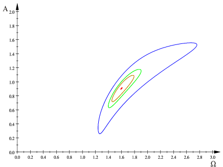
Figure 1: Amplitude profiles $A\left(\Omega\right)$, $\gamma=\gamma_{\ast}$, $h=0.4$ (blue), $0.8$ (green), $0.85$ (sienna), $h_{\ast}$ (red).

Figure 2: Bifurcation diagram for the Duffing equation, $h=0.4,\ \gamma=\gamma_{\ast}$.

Resonance $1:3$ is shown in Fig. 2 where bifurcation diagram for the Duffing equation (10) in $\left(z,\ \Omega\right)$ plane was computed for $h=0.4,\ \gamma=\gamma_{\ast}$ and $\Omega\in\left[2.3,\ 3.0\right]$.

Since the KBM method is approximate metamorphosis in the real system may happen at a slightly different value of, say, parameter $h$. The numerically exact critical value of this parameter was determined from the bifurcation diagram below where dependence of $z$ on $h$ is shown for $\Omega=\Omega_{\ast}$, $\gamma=\gamma_{\ast}$.

Figure 3: Bifurcation diagram for the Duffing equation, $\Omega=\Omega_{\ast}$, $\gamma=\gamma_{\ast}$.

It follows that the $1:3$ resonance ends abruptly for growing $h$ at $h\cong 0.905$, i.e. slightly above the critical value $h_{\ast}$.

In Figs. 4, 5 below bifurcations diagrams showing dependence of $z$ on $\Omega$ for $\gamma=\gamma_{\ast}$ and $h=0.90,\ 0.92$ are shown.

Figure 4: Bifurcation diagram for the Duffing equation, $h=0.9,\ \gamma=\gamma_{\ast}$.

We realize that the $1:3$ resonance disappears for growing $h$ in agreement with analytical computations (based however on the approximate KBM method).

Figure 5: Bifurcation diagram for the Duffing equation, $h=0.92,\ \gamma=\gamma_{\ast}$.

6 Summary and discussion

In this work we have studied metamorphoses of amplitude profiles for the $1:3$ resonances of the effective equation, describing approximately dynamics of two coupled periodically driven oscillators. Our analysis has been analytical although based on the approximate KBM method. Theory of algebraic curves has been used to compute singular points on amplitude profiles of the effective as well as the Duffing equation. It follows from general theory that metamorphoses of amplitude profiles occur in neighbourhoods of such points. The results obtained can be compared with our work on metamorphoses of $1:1$ resonances in the effective equation [10].

In Section 4 we have computed analytically positions of singular points for the amplitude profiles $A\left(\Omega\right)$ determined within the Krylov-Bogoliubov-Mitropolsky approach for the approximate 2nd-order effective equation (9). In Section 5 analytical and numerical results have been presented for the case of the Duffing equation arising as the subsequent approximation of the effective equation. We have also computed numerically bifurcation diagrams in the neighbourhoods of singular points and indeed dynamics of the Duffing equation (10) changes according to metamorphoses of the corresponding amplitude profiles. More exactly, we have found only the case of isolated singular point and this corresponds to creation or destruction of $1:3$ resonance. We are going to investigate much more complicated case of the effective equation in our next paper.

References

• [1] J. P. Den Hartog, Mechanical Vibrations (4th edition), Dover Publications, New York 1985.
• [2] S. S. Oueini, A. H. Nayfeh and J.R. Pratt, Arch. Appl. Mech. 69, 585 (1999).
• [3] W. Szemplińska-Stupnicka, The Behavior of Non-linear Vibrating Systems, Kluver Academic Publishers, Dordrecht, 1990.
• [4] J. Awrejcewicz, Bifurcation and Chaos in Coupled Oscillators, World Scientific, New Jersey 1991.
• [5] J. Kozłowski, U. Parlitz and W. Lauterborn, Phys. Rev. E 51, 1861 (1995).
• [6] K. Janicki, W. Szemplińska-Stupnicka, J. Sound. Vibr. 180, 253 (1995).
• [7] A. P. Kuznetsov, N. V. Stankevich and L. V Turukina, Physica D 238, 1203 (2009).
• [8] A. Okniński and J. Kyzioł, Differential Equations and Nonlinear Mechanics 2006, Article ID 56146 (2006).
• [9] J. Kyzioł, PhD Thesis, Kielce University of Technology, 2007.
• [10] J. Kyzioł, and A. Okniński, Acta Phys. Polon. B 42, 2063 (2011); arXiv:1012.2140v1[nlin.CD].
• [11] A. H. Nayfeh, Introduction to Perturbation Techniques, John Wiley & Sons, New York 1981.
• [12] J. Awrejcewicz and V.A. Krysko, Introduction to Asymptotic Methods. Chapman and Hall (CRC Press), New York 2006.
• [13] N. N. Bogoliubov, Y. A. Mitropolsky, Asymptotic Methods in the theory of Nonlinear Oscillators, Gordon and Breach, New York 1961.
• [14] C. T. C. Wall, Singular Points of Plane Curves, Cambridge University Press, New York 2004.