Sensing Matrix Setting Schemes for Cognitive Networks and Their Performance Analysis

Abstract

Powerful spectrum decision schemes enable cognitive radios (CRs) to find transmission opportunities in spectral resources allocated exclusively to the primary users. One of the key effecting factor on the CR network throughput is the spectrum sensing sequence used by each secondary user. In this paper, secondary users’ throughput maximization through finding an appropriate sensing matrix (SM) is investigated. To this end, first the average throughput of the CR network is evaluated for a given SM. Then, an optimization problem based on the maximization of the network throughput is formulated in order to find the optimal SM. As the optimum solution is very complicated, to avoid its major challenges, three novel sub optimum solutions for finding an appropriate SM are proposed for various cases including perfect and non-perfect sensing. Despite of having less computational complexities as well as lower consumed energies, the proposed solutions perform quite well compared to the optimum solution (the optimum SM). The structure and performance of the proposed SM setting schemes are discussed in detail and a set of illustrative simulation results is presented to validate their efficiencies.

I Introduction

Opportunistic spectrum sharing has been developed through the new promising concept of Cognitive Radio (CR), in order to meet ever-growing spectrum demands for new wireless services. Conceptually, CR is an adaptive communication system which offers the promise of intelligent radios that can learn from and adapt to their environment [1]. The major issue in designing a cognitive radio network is to protect incumbent/primary users from potential interference problems while providing acceptable quality-of-service (QoS) levels for secondary users (i.e., unlicensed users). To this end, sensing capability is exploited in CRs which enable them to find some transmission opportunities called white spaces, i.e., temporarily-available spectrums which are not used by primary users (PUs). Limited number of possible observations and dynamic nature of observed signals lead to imperfect sensing which is usually described by false alarm and miss detection probabilities. The false alarm occurs when the PU is idle, but the Secondary User (SU) senses the channel as busy. While the miss detection is occurred when the SU senses an occupied channel as free.

Average throughput of the SUs is one of the most important performance metrics which depends on the candidate primary channels for sensing and transmission, and it must be considered in designing appropriate sensing schemes. Generally, there exists more than one channel to be sensed by a CR. As a result, sensing schemes are commonly divided into two categories, i.e., wideband sensing and narrowband sensing. Sensing is wideband when multiple channels are sensed simultaneously. These multiple sensed channels can cover either the whole or a portion of the primary channels [2]. On the other hand, when only one channel is sensed at a time, the sensing is narrowband. Ease of implementation, lower power consumption, and less computational complexity lead to great interest in narrowband sensing. When the narrowband sensing is used, an immediate question arises: which channel should be sensed first? In other words, to achieve the best possible performance, the channels have to be sensed in an appropriate order determined by sensing sequence (SS).

In [3], the problem of joint optimization of sensing and transmission is addressed. Specifically, Zhao et al. in [3] proposed a decentralized slotted CR MAC protocol to grasp the optimal policies for spectrum sensing and access framework through a partially observable Markov decision process. Minimizing the overall system time of a SU, which contains the average waiting time and the extended data delivery time, through load balancing in probability-based and sensing-based spectrum decision schemes is investigated in [4]. In [5], [6], and [7], the procedures to determine the optimal set of candidate channels for sensing are first discussed and then the maximization of the spectrum accessibility through optimal number of candidate channels are investigated. In [8], [9], and [10], the sequential channel sensing problems are formulated based on maximizing the throughput of the SUs. While in these works, the optimum sensing times have been studied, the effects of the sensing errors have not been addressed. Setting a SS by prioritizing the various channels can play a major role in finding a transmission opportunity or equivalently expected SU’s throughput. Channel prioritization has been considered in [11] in which an optimal channel sensing framework for a single-user case including the sensing order and the stopping rule has been proposed. In [11], it has been also assumed that the SUs are allowed to recall and guess. Recall means the ability to go back and access a previously sensed channel and guess means accessing a channel that has not been sensed yet. In [12] and [13], a stopping rule has been developed to determine when to stop the sequential sensing procedure and when to start secondary transmission. In [14], the optimal SS has been derived for channels with homogeneous capacities, and it was shown that the problem of finding the optimal sensing sequence for these channels is NP-hard. The authors in [15] have suggested a SS which sorts channels in descending order according to their idle probabilities. In [16], finding the optimal SS sequence has been investigated for a single-user case with the aim to maximize the SU’s throughput. The problem of finding optimal SS for two CR users has been addressed in [17], in which an exhaustive search has been applied in order to find the best sensing sequences for the users at the expense of a huge computational complexity. To reduce the complexity associated with the optimum solution, the authors of [17] have proposed two low-complexity suboptimal algorithms with the achieved throughput close to the maximum possible value.

In this paper, the problem of selecting proper spectrum sensing sequences for a cognitive radio network (CRN) with multiple users is addressed. Our objective is to maximize the average network throughput. First, we assume a perfect channel sensing (i.e., error-free sensing) and formulate an optimization problem on spectrum sensing sequences of the SUs based on maximizing the average throughput of the network. We discuss the conventional solution as well as its computational complexity. Due to massive computational burden of the conventional optimization algorithm, a novel algorithm, which finds near-optimal solution, is proposed. The proposed algorithm, called sensing matrix setting (SMS), provides short-term and mid-term fairness among the SUs and offers near-optimal solution with tolerable computational complexity as well as relatively low consumed energy. Then, we consider the impact of sensing error on the SMS algorithm, and propose modified version of SMS algorithm, called MSMS algorithm. In addition, for the multiple access among the SUs, we apply the conventional p-persistent MAC within the MSMS algorithm, and call the extended algorithm as PMSMS algorithm. Structure, performance, and related spectrum allocation processes for the proposed algorithms are discussed in detail.

The rest of this paper is organized as follows. In Section II, we describe the CR network considered and the related assumptions. In Section II, the throughput of the CRN for a given sensing matrix is formulated, and the conventional approach to find the optimal SM as well as its computational complexity are discussed. In Section IV, the structure, computational complexity, and consumed energy of the novel suboptimal SMS algorithm are described in detail. In Section V, the modified version of the SMS algorithm is introduced. The PMSMS algorithm is described in Section VI. Numerical results are then presented in Section VII, which validate our analysis and verify the advantages of the proposed algorithms. Finally, the paper is concluded in Section VIII.

II System Model

We assume a time slotted CRN with $N_{s}$ secondary users which attempt to opportunistically transmit in the channels dedicated to the $N_{p}$ PUs. As in [13], [16], [17], and [18], the SUs are time synchronous in time-slots with other SUs and with the PUs. When a PU has no data for transmission, it does not use its time-slots; and hereby provides a transmission opportunity for the SUs. That is, at the beginning of each time-slot, a channel can be established as occupied or vacant. In order to find the transmission opportunities appropriately and to protect the PUs from harmful interference, the sensing process is performed at the beginning of each time-slot. We assume that the SUs are equipped with simple transceivers, so they are able to sense only one channel at a time. The SUs always have packets to transmit, and as a consequence they will start transmission when an opportunity is found. Each SU senses the channels according to its SS sequentially, i.e., the SU senses the first channel from the top of its SS for a predetermined time duration (channel sensing time), and then senses the second channel if and only if the first channel is found busy. This procedure will continue until a transmission opportunity is found. Moreover, as [16], we assume that the SUs are not able to ”recall” which means that they cannot re-sense and transmit on a previously sensed busy channel.

The SU might stop its transmission in a channel and try to choose a new one due to the presence of the PU or the availability of a better channel with a more appropriate transmission condition. In order to switch to a new channel, which is called spectrum Hand-Over (HO), a secondary device needs a specific and constant time duration $\tau_{ho}$ to prepare its sensing circuitry for the next spectrum sensing.

For the SU, each slot contains two phases: 1) sensing phase, and 2) transmission phase. The sensing phase contains several mini-slots of duration $\tau$ (sensing time of each channel). Sensing is carried out by the SUs in the mini-slots, and once the transmission opportunity is found, the transmission phase will be started. This kind of access, i.e., listen-before-talk (LBT), is a common method in many wireless communication systems, for example see the quiet period in IEEE 802.22 standard [19]. The sensing procedure is performed in an order based on the SS provided by the secondary network coordinator. The SUs do not have the adaptive modulation and coding (AMC) capability; so they transmit with a constant rate, $R$, during the transmission phase. We define a sensing matrix (SM) as a matrix with the dimensions of ${N_{s}}\times{N_{p}}$, in which the $i$-th row contains the SS dedicated to the $i$-th SU. Given the primary-free probabilities, i.e., ${P_{0,j}}{\rm{~{}}},{\rm{~{}}}1\leq j\leq{N_{p}}$, and predetermined false alarm and detection probabilities, our objective is to find the optimal (or near-optimal) SS of each SU, i.e., the optimal SM, in order to maximize the CRN throughput.

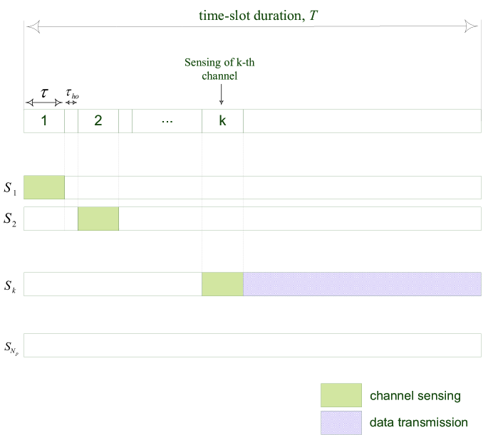
Figure 1: General timing structure of our system model.

Fig. 1 demonstrates the slotted timing structure of a SU and its sensing process. For the example considered in Fig. 1, after sensing $\left(k-1\right)$ occupied channels, the SU senses the $k$-th channel free and then transmits data on that channel until the end of the slot. The wasted time length, i.e., the time allocated for sensing and HO in this process is equal to $\tau+\left(k-1\right)\left(\tau+\tau_{ho}\right)$. Thus, the time left in the slot for transmission is $T-\tau-\left(k-1\right)\left(\tau+\tau_{ho}\right)$, where $T$ is the time slot duration. Generally speaking, each slot is composed of a sensing phase with the maximum length of $\tau+\left(N_{p}-1\right)\left(\tau+\tau_{ho}\right)$ and a transmission phase with the minimum length of $T-\tau-\left(N_{p}-1\right)\left(\tau+\tau_{ho}\right)$. Let us define the slot effectiveness, denoted by $e_{s}$, as the ratio of the transmission phase length to the slot length. Hence, if a secondary user starts transmitting on the $k$-th channel of its SS, the slot effectiveness is:

$$e_{s}=\frac{transmission~{}time}{time~{}slot~{}duration}=1-\frac{\tau+\left(k-1\right)\left(\tau+\tau_{ho}\right)}{T}$$ (1)

and

$$B_{k}=R\times e_{s}=R\left(1-\frac{\tau+\left(k-1\right)\left(\tau+\tau_{ho}\right)}{T}\right)$$ (2)

where $B_{k}$ is the average throughput of the SU if the $k$-th channel of the SS is sensed to be free and chosen for the transmission. From (1) by the increase of $k$, the channel effectiveness is reduced.

III Optimal Sensing Matrix

In this section, we evaluate the CRN throughput for error-free sensing case and discuss about the optimal sensing sequences of the SUs (or equivalently SM) for the network throughput maximization. The optimal sensing sequence for the CRN containing just one SU is derived in [15]. For that case, all required was to sort the spectrums based on their primary-free probabilities (i.e., the absence probability of the PU). But in the CRN with multi users, the impact of collisions among the SUs’ transmissions has to be taken into account. Assume that $S$ denotes the sensing matrix which contains $N_{s}$ rows and $N_{p}$ columns with the element $s_{i,j}$ indicating that the $i$-th SU senses the $s_{i,j}$-th spectrum in its $j$-th mini-slots.

For network throughput evaluation, we note that for each spectrum $s_{i,j}$ two possible cases might occur. First, the $s_{i,j}$-th spectrum has been sensed by some SUs in their previous mini-slots (the mini-slots before $j$-th mini-slot). In this case, regardless of the presence or the absence of the PU, the spectrum is occupied (as we assumed error-free sensing in this section). That is, the SU that senses this channel at the first time will transmit on the channel, as a result of perfect sensing, if the spectrum is idle. Second, the spectrum is sensed at the $j$-th mini-slot by $i$-th SU at the first time. So, the occupation probability of this channel only depends on the PU activity. If the $s_{i,j}$ is sensed free, the $i$-th SU starts its transmission in this spectrum for the rest of the time slot with a constant rate $R$. From the above discussion, repetition of a spectrum in the sensing matrix when assuming error-free sensing does not offer any benefit to the CRN throughput.

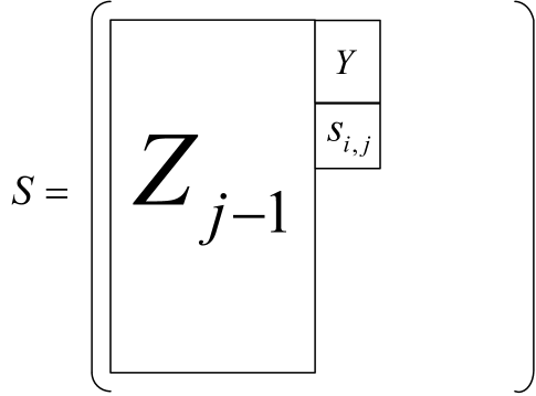
Figure 2: Graphical representation of the sensing matrix.

Fig. 2 shows the structure of the SM. In this Fig., $Z_{j-1}$ demonstrates the spectrums allocated prior to the $j$-th mini-slot. The array $Y$ contains the spectrums dedicated at the $j$-th mini-slot to the SUs prior to the user $i$. Let $A_{{s_{i,j}}}^{{Z_{j-1}}}$ indicate the presence or absence of the spectrum $s_{i,j}$ in $Z_{j-1}$,

$$A_{{s_{i,j}}}^{{Z_{j-1}}}=\left\{{\begin{array}[]{*{20}{c}}{0{\text{~{}:~{}}}if{\text{~{}}}{s_{i,j}}\in{Z_{j-1}\hfill}}\\ {1{\text{~{}:~{}}}if{\text{~{}}}{s_{i,j}}\notin{Z_{j-1}\hfill}}\\ \end{array}}\right.$$ (3)

By the above definition, when not taking into account the impact of collision caused by multi SU transmissions at the same spectrum due to simultaneously finding the spectrum free at the $j$-th mini-slot, the spectrum $s_{i,j}$ can be efficiently used by the $i$-th SU with the probability of ${P_{0,{s_{i,j}}}}A_{{s_{i,j}}}^{{Z_{j-1}}}$, where $P_{0,{s_{i,j}}}$ is the absence probability of the $s_{i,j}$-th PU. To consider the impact of the collision on the network throughput as discussed above, we define the operator $\oplus$ as follows.

$$\oplus:\left\{{\begin{array}[]{*{20}{c}}{A\oplus B=B\oplus A\hfill}\\ {A\oplus B\oplus C=A\oplus C\oplus B=B\oplus C\oplus A\hfill}\\ {\forall m\leqslant{N_{p}}:{P_{0,{s_{1}}}}{A_{{s_{1}}}^{{Z_{j-1}}}}\oplus{P_{0,{s_{2}}}}{A_{{s_{2}}}^{{Z_{j-1}}}}\oplus\cdots\oplus{P_{0,{s_{m}}}}{A_{{s_{m}}}^{{Z_{j-1}}}}=\mathchar 22\relax\mkern-10.0mu\lambda\hfill}\\ \end{array}}\right.$$ (4)

where

$$\mathchar 22\relax\mkern-10.0mu\lambda=\left\{{\begin{array}[]{*{20}{c}}0&{{\text{iff~{}}}{s_{1}}={s_{2}}=\cdots={s_{m}}}\\ {{P_{0,{s_{1}}}}{A_{{s_{1}}}^{{Z_{j-1}}}}+{P_{0,{s_{2}}}}{A_{{s_{2}}}^{{Z_{j-1}}}}+\cdots+{P_{0,{s_{m}}}}{A_{{s_{m}}}}^{{Z_{j-1}}}}&{{\text{iff~{}}}{s_{1}}\neq{s_{2}}\neq\cdots\neq{s_{m}}}\\ \end{array}}\right.$$ (5)

The operator $\oplus$ is used to model the possible collision due to multi SUs finding the same spectrum free at the $j$-th mini-slot. As stated before, each channel in each time-slot has a contribution in the whole throughput if and only if it is sensed only by one SU (i.e., assigned to one SU sensing sequence) because of error-free sensing assumption.

By the above definition of the operator $\oplus$, the average throughput of the CRN is easily computed as follows,

$$\begin{gathered}Q=\left({{P_{0,{s_{1,1}}}}A_{{s_{1,1}}}^{{Z_{0}}}\oplus{P_{0,{s_{2,1}}}}A_{{s_{2,1}}}^{{Z_{0}}}\oplus\cdots\oplus{P_{0,{s_{{N_{s}},1}}}}A_{{s_{{N_{s}},1}}}^{{Z_{0}}}}\right){B_{1}}+\\ {\text{ }}\left({{P_{0,{s_{1,2}}}}A_{{s_{1,2}}}^{{Z_{1}}}\oplus{P_{0,{s_{2,2}}}}A_{{s_{2,2}}}^{{Z_{1}}}\oplus\cdots\oplus{P_{0,{s_{{N_{s}},2}}}}A_{{s_{{N_{s}},2}}}^{{Z_{1}}}}\right){B_{2}}+\cdots+\\ {\text{ }}\left({{P_{0,{s_{1,{N_{p}}}}}}A_{{s_{1,{N_{p}}}}}^{{Z_{{N_{p}}-1}}}\oplus{P_{0,{s_{2,{N_{p}}}}}}A_{{s_{2,{N_{p}}}}}^{{Z_{{N_{p}}-1}}}\oplus\cdots\oplus{P_{0,{s_{{N_{s}},{N_{p}}}}}}A_{{s_{{N_{s}},{N_{p}}}}}^{{Z_{{N_{p}}-1}}}}\right){B_{{N_{p}}}}\\ \end{gathered}$$ (6)

where $B_{j}$ is defined in (2) and $A_{{s_{i,1}}}^{{Z_{0}}}\triangleq 1{\text{~{},}}\forall i\leqslant{N_{p}}$. Now, the optimal SM is found by solving the following optimization problem,

$${S^{*}}=\mathop{\arg\max}\limits_{{s_{1,1}},{s_{1,2}},\ldots,{s_{{N_{s}},{\text{~{}}}{N_{p}}}}}{\text{~{}Q}}$$ (7)

Based on the derived optimization problem, we can find the optimal SM by exploiting exhaustive search. Assume that the computational complexity of computing (6) for a given SM, $S$, is in $\mathcal{O}\left(1\right)$. Then, the computational complexity of finding the optimal SM is in $\mathcal{O}\left({{N_{p}}^{{N_{p}}\times{N_{s}}}}\right)$. Since the expression describing the performance metric (the CRN throughput) is complicated in general, there is no much room for solving (7) through classical optimization procedures. On the other hand, solving (7) through the exhaustive search makes no guarantee for fairness among the SUs. In addition, it results in massive computational burden which is not scalable regarding to both $N_{p}$ and $N_{s}$. All these facts make a strong motivation and interest in developing an appropriate suboptimal solution for the problem formulated in (7). In the following sections, we propose suboptimum solutions for the SM for three different cases. Advantages of proposed algorithms are threefold: First, it offers low computational complexity. Second, it provides fairness among the SUs. Finally, its consumed sensing energy to find a transmission opportunity is much less than the exhaustive search.

IV SMS Algorithm

IV-A Structure of the SMS Algorithm

The proposed algorithm, designed for error-free sensing case, is composed of $N_{p}$ rounds. In the $k$-th round, the coordinator determines the $k$-th column of the SM, i.e., $s_{i,k},~{}1\leq i\leq{N_{s}}$. As mentioned before, repeating a spectrum in the SM for more than one times either in the same mini-slot or in different mini-slots does not have any benefits on the network throughput. During each round and for each SU, the coordinator assigns a reward to each candidate channel to be possibly allocated to the SS of the SU at that round and then adopts the channel with the maximum reward. That is, at the round $m$, for each secondary user $k$ and for each unassigned channel $i$, we define $G_{i}^{\left(k\right)}\left(m\right)$ as the reward of the channel $i$ if selected as the $m$-th component of the $k$-th SU’s sensing sequence. This reward is set equal to the contribution of the $k$-th SU to the network throughput if the $i$-th channel is selected, as will be described latter. Then, the channel with the maximum reward is selected.

We denote the set of all assigned channels to the sensing matrix by $A$. At the beginning, we have $A=\emptyset$ and $S=\emptyset$ ,where $S$ is the sensing matrix and $\emptyset$ denotes empty matrix. We also denote the set of all channels by $\mathbb{N}$, where $\mathbb{N}=\left\{{1,2,\ldots,{N_{p}}}\right\}$. The process is as follows:

Round-1

For this round, first the coordinator assigns a spectrum to the SS of the first SU at its first mini-slot. The coordinator must adopt $s_{1,1}$ from the unassigned channels, i.e., $\overline{A}=\mathbb{N}\backslash A=\mathbb{N}$. We have $G_{i}^{\left(1\right)}\left(1\right)={P_{0,i}}{B_{1}}$, where $B_{1}$ is defined in (2). The coordinator selects a channel with the highest reward for the $s_{1,1}$. That is, the first channel to be sensed by the first SU is,

$${s_{1,1}}=\mathop{\arg\max}\limits_{i\in\overline{A}}{\text{~{}}}G_{i}^{\left(1\right)}\left(1\right)$$ (8)

After $s_{1,1}$ is determined, $A$ and $\overline{A}$ are respectively updated to $A=\left\{{{s_{1,1}}}\right\}$ and $\overline{A}=\mathbb{N}\backslash A$. This procedure is repeated for each SU; so for the $\ell$-th user in the first round, we have,

$${s_{\ell,1}}=\mathop{\arg\max}\limits_{i\in\overline{A}}{\text{~{}}}G_{i}^{\left(\ell\right)}\left(1\right)$$ (9)

where $G_{i}^{\left(\ell\right)}\left(1\right)={P_{0,i}}{B_{1}}$.

Round-m

At the $m$-th round, for each SU, the coordinator similarly assigns a reward to each left spectrums and allocates the best spectrum, which has the maximum reward, to the SU. If the coordinator chooses the $j$-th channel for the $m$-th sensing mini-slot of the $\ell$-th SU, the following reward will be gained by the user.

$$G_{j}^{\left(\ell\right)}\left(m\right)=\left({\prod\limits_{i=1}^{m-1}{\left({1-{P_{0,{s_{\ell,i}}}}}\right)}}\right){P_{0,j}}{B_{m}}$$ (10)

Hence, the coordinator determines the $m$-th element of the SS of the $\ell$-th SU as,

$${s_{\ell,m}}=\mathop{\arg\max}\limits_{i\in\overline{A}}{\text{~{}}}G_{i}^{\left(\ell\right)}\left(m\right)$$ (11)

At this round, first it must be determined from which SU the procedure should be started. In order to achieve an acceptable level of fairness among the SUs, the algorithm starts with a SU that has gained the lowest cumulative rewards during the previous $\left(m-1\right)$ rounds (previous $\left(m-1\right)$ mini-slots). The cumulative reward gained during the previous $\left(m-1\right)$ mini-slots is calculated for the $\ell$-th SU as,

$$\sum\limits_{k=1}^{m-1}{G_{{s_{\ell,k}}}^{\left(\ell\right)}\left(k\right)}=G_{{s_{\ell,1}}}^{\left(\ell\right)}\left(1\right)+G_{{s_{\ell,2}}}^{\left(\ell\right)}\left(2\right)+\cdots G_{{s_{\ell,m-1}}}^{\left(\ell\right)}\left({m-1}\right)$$ (12)

where ${G_{{s_{\ell,k}}}^{\left(\ell\right)}\left(k\right)}$ is defined in (10).

This process continues until $\left|A\right|={N_{p}}$ or equivalently $\overline{A}=\emptyset$. At the end of the process, the elements of $S$ without any assigned spectrum are replaced by zero, which indicates that the sensing is not performed for those elements. Since each channel is sensed only once in the proposed algorithm, the energy consumed by the SMS algorithm equals to $N_{p}E_{c}$ at the worst case, and it does not increase by $N_{s}$.

In order to have mid-term fairness, at the beginning of second time-slot, the process starts with the second SU and the first element of the sensing sequence of this user is determined and then the procedure is continued by selecting the first element of the third user, and at the last the first element of the first user is selected. The other elements are determined as described above. This cyclic ordering is continued in the following time-slots, i.e., at the beginning of $m$-th run of the SMS procedure ($m$-th time-slot) the process starts with selecting the first element of the sensing sequence of the $k$-th SU, where

$$k=\bmod\left({m,{N_{p}}}\right)$$ (13)

These procedures are summarized in Algorithm 1.

Algorithm 1 sensing matrix setting algorithm for perfect sensing case(the SMS algorithm)

  Initialization: $S=\emptyset$, $\mathbb{N}=\left\{{1,2,\ldots,{N_{p}}}\right\}$, $A=\emptyset$, $\overline{A}=\mathbb{N}\backslash A$, and $m=1$

  $H\leftarrow$ sort the SUs based on their numbers, sequentially.

  for $m=1$ to (the maximum number of the SUs’ mini-slots) do

     for $\ell=$ (the first element of $H$) to (the last element of $H$) do

        for $i=1$ to $N_{p}$ do

           if $\overline{A}\neq\emptyset$ then

              Compute $G_{i}^{\left(\ell\right)}\left(m\right)$ as in (10)

              Assign ${s_{\ell,m}}\leftarrow\mathop{\arg\max}\limits_{i\in\overline{A}}{\text{~{}}}G_{i}^{\left(\ell\right)}\left(m\right)$

           else

              ${s_{\ell,m}}\leftarrow 0$

           end if

        end for

        if ${\text{the~{}spectrum~{}}}i{\text{~{}is~{}assigned~{}to~{}}}{s_{\ell,m}}$ then

           Add $\left\{i\right\}$ to $A$

           Update $\overline{A}$

        end if

     end for

     $H\leftarrow$ sort the SUs based on their cumulative rewards computed using (12).

  end for

  Return $S$ as the suboptimal sensing matrix.

IV-B Computational Complexity

As we stated before, the computational complexity of finding the optimal SM is in order of $\mathcal{O}\left({{N_{p}}^{{N_{p}}\times{N_{s}}}}\right)$, while it is in order of $\mathcal{O}\left(1\right)$ for our proposed method. In the SMS algorithm, a channel will be assigned to the SM if it offers the highest reward, defined in (10), among the left channels. From (10), it can be easily shown that ${G_{j}}^{(l)}\left(m\right)>{G_{k}}^{(l)}\left(m\right)$ if ${P_{0,j}}>{P_{0,k}}$ . So for the the error-free case, the information required to determine the SM is the primary-free probabilities of the channels.

IV-C Averaged Consumed Energy for Finding a Transmission Opportunity

Let $E_{c}\left(\tau\right)$ and $E_{c}\left(\tau_{ho}\right)$ denote the consumed energy for sensing of each primary channel and the consumed energy for each HO, respectively. Hence, the average consumed energy for finding a transmission opportunity can be calculated as,

$$\left({N_{s}+{{\bar{g}}_{1}}+{{\bar{g}}_{2}}+\cdots+{{\bar{g}}_{{N_{s}}}}}\right){E_{c}}\left(\tau\right)+\left({{{\bar{g}}_{1}}+{{\bar{g}}_{2}}+\cdots+{{\bar{g}}_{{N_{s}}}}}\right){E_{c}}\left({{\tau_{ho}}}\right)$$ (14)

where ${{{\bar{g}}_{i}}}$ denotes the average number of HOs required by the $i$-th SU to find an idle channel.

The processes of channel sensing and signal transmission consume more energy compared to the HO. Therefore, it is rational to ignore the second term $\left({{{\bar{g}}_{1}}+{{\bar{g}}_{2}}+\cdots+{{\bar{g}}_{{N_{s}}}}}\right){E_{c}}\left({{\tau_{ho}}}\right)$ in (14) compared to the first one.

To evaluate the average number of HOs of the $i$-th SU, ${{{\bar{g}}_{i}}}$, we consider two following cases: 1) The SU searches among the channels, finds a transmission opportunity, and then transmits, 2) The SU searches among the available channels, but does not find any free channel. Then, ${{{\bar{g}}_{i}}}$ can be easily calculated as,

$${\overline{g}_{i}}={\underbrace{{P_{1,s_{i,1}}}{P_{0,s_{i,2}}}+2{P_{1,s_{i,1}}}{P_{1,s_{i,2}}}{P_{0,s_{i,3}}}+\cdots+\left(N_{p}-1\right)P_{0,s_{i,N_{p}}}\prod\limits_{j=1}^{N_{p}-1}{P_{1,s_{i,j}}}}_{T1}}+N_{p}\prod\limits_{j=1}^{N_{p}}{{P_{1,s_{i,j}}}}$$ (15)

where the term $T1$ represents the average sensed channels by the $i$-th SU until the user finds a transmission opportunity, and the last term demonstrates the case that the SU senses all channels busy, and therefore it does not transmit on any channels assigned to its SS. By substituting (15) in (14), the total average consumed energy for the exhaustive search method is derived as follows:

$$\sum\limits_{i=1}^{{N_{S}}}{{{\bar{g}}_{i}}}{E_{C}}={E_{C}}\sum\limits_{i=1}^{{N_{S}}}{\left(1+\sum\limits_{k=2}^{{N_{P}}}{\left({\left({k-1}\right)\prod\limits_{j=1}^{k-1}{{P_{1,{s_{i,j}}}}}}\right){P_{0,{s_{i,k}}}}}\right)}+{E_{C}}\sum\limits_{i=1}^{{N_{S}}}{{N_{p}}\prod\limits_{j=1}^{{N_{P}}}{{P_{1,{s_{i,j}}}}}}$$ (16)

On the other hand, for the SMS algorithm, analytically deriving the average consumed energy is complicated. Hence, we only focus on two special extreme case, i.e., the maximum and minimum consumed energies. For the worst case, which consumes the maximum energy, all the channels appeared in the SM are sensed. In this case, the consumed energy equals to ${N_{p}}{E_{C}}\left(\tau\right)$. For the best case, which consumes the minimum energy, each SU finds the first channel of its SS free and does not need to sense the rest. In this case, the consumed energy is equal to $\min\left({{N_{p}},{N_{s}}}\right){E_{C}}\left(\tau\right)$. It is worth noting that for ${P_{0,j}}=1~{},for~{}all~{}j$, the sequential sensing scheme forces the SUs to continue searching among all channels in their sensing sequences, which is equivalent to the worst case, and similarly ${P_{0,j}}=0~{},for~{}all~{}j$ is equivalent to the best case with minimum consumed energy. If we compute the average consumed energy of the optimum solution given in (16) for theses two cases, the maximum and minimum consumed energies will be equal to ${E_{C}}{N_{s}}\left({1+{N_{p}}}\right)$ and ${E_{C}}{N_{s}}$, respectively, which are higher than those of the SMS algorithm.

For more elaboration, we study an especial case where all channels have the same primary-free probabilities, i.e., ${P_{0,j}}=P{\text{~{}}},{\text{~{}~{}}}{P_{1,j}}=1-P{\text{~{}}},for~{}all~{}j$. Then, we can simplify (16) as follows,

$$\begin{gathered}{E_{C}}\left(\tau\right)\sum\limits_{i=1}^{{N_{S}}}{{{\bar{g}}_{i}}}={E_{C}}\left(\tau\right)\left({{N_{S}}P+P\sum\limits_{i=1}^{{N_{S}}}{\left({\sum\limits_{k=2}^{{N_{p}}}{\left({\left({k-1}\right){{\left({1-P}\right)}^{k-1}}}\right)}}\right)+}{N_{S}}{N_{p}}{{\left({1-P}\right)}^{{N_{p}}}}}\right)\\ ={E_{C}}\left(\tau\right){N_{S}}\left({P+\frac{{1-P+\left({-1+P-P{N_{p}}}\right){{\left({1-P}\right)}^{{N_{p}}}}}}{P}+{N_{p}}{{\left({1-P}\right)}^{{N_{p}}}}}\right)\\ ={E_{C}}\left(\tau\right){N_{S}}\left({\frac{{{{\left({1-P}\right)}^{2}}-{{\left({1-P}\right)}^{{N_{p}}+1}}}}{P}+1}\right)\\ \end{gathered}$$ (17)

It is worth noting that (17) is a decreasing function of $P$. Hence, the minimum and maximum values of consumed energy are related to the cases $P=0$ and $P=1$, as discussed above. Moreover, as will be shown in the numerical result section (Fig. 5), the consumed energy associated with the optimal SM is higher than the consumed energy for the matrix obtained by the SMS algorithm for all values of $P$.

In the following, the impacts of the sensing errors are investigated. In general, the sensing error manifests itself in two forms: false alarm and miss-detection. In the SMS algorithm proposed, a channel is allocated to only one SS, and thus the SUs have no common channels in their sequences. Although this approach performs well when there is no sensing error, but in the case of non-perfect sensing, this method is not efficient; since by a false alarm made by a SU in a sensed channel, a transmission opportunity is lost for this channel by all SUs. Therefore, it seems that the coordinator has to repeat spectrums in the $S$ in order to increase the possibility of exploiting all opportunities and thus to increase the spectral efficiency. On the other hand, allocating a channel to the sensing sequences of multiple SUs increases the average number of sensed channels and thus raises the average sensing energy consumption. Moreover, due to miss-detection, it is possible for a SU to mistakenly transmit on a channel which is already used by another SU or PU, and therefore some collisions might occur. Hence, there is a trade-off between the average achievable throughput, energy consumption, and the level of collision in the CRN which must be addressed in an extension of the SMS algorithm.

To modify the SMS algorithm, we must consider the impact of sensing error probabilities on the reward function. Moreover, the channels occupation probabilities will be different at the beginning of the various mini-slots, which must be reflected in the reward function. Finally, because of repetition of each channel in the SM, the stopping rule, which was $\left|A\right|={N_{p}}$, must be modified.

V MSMS Algorithm

Since in the SMS algorithm, the sensing sequences of the SUs have no common channels, the occupancies of channels at the beginning of each mini-slot only depend on the PUs’ activities. But if the channels are allowed to be repeated in multiple rows or columns of the SM, the occupancy of a channel can be due to the presence of either the PU or a SU. To extend the SMS algorithm, first the occupation probability of the $j$-th channel, i.e., ${q_{1,j}}$, has to be determined.

It is worth noting that, since all the SUs use the same sensing schemes with the same sensing time lengths, they all have the same probabilities of false alarm and miss-detection. Thus, we have,

$$\begin{gathered}{P_{fa,1}}={P_{fa,2}}=\cdots={P_{fa,{N_{p}}}}={P_{fa}}\hfill\\ {P_{d,1}}={P_{d,2}}=\cdots={P_{d,{N_{p}}}}={P_{d}}\hfill\\ \end{gathered}$$ (18)

In order to reflect the impact of sensing error on the proposed algorithm, three possible cases must be considered when the coordinator tends to adopt the $l$-th channel as $s_{i,j}$:

• The $l$-th channel has not yet been allocated to any sensing sequences, i.e., $l\notin{Z_{j-1}}$ (matrix Z is defined in section III and Fig. 2).

• The $l$-th channel has been adopted at least once for sensing at the previous mini-slots, i.e., $l\in{Z_{j-1}}$.

• The $l$-th channel has been allocated simultaneously to multiple users at the $j$-th mini-slot (vector $Y$ shown in Fig. 2).

Fig. 2 depicts these cases graphically. Suppose that $j$-th component of the SS of the $i$-th SU, i.e., $s_{i,j}$, is to be selected by the coordinator. So the reward gained by adopting the $k$-th channel as $s_{i,j}$ is to be determined. Considering the definition of the matrix $Z$ and the vector $Y$ in Section III and also in Fig. 2, if $n$ elements of $Z$ are equal to $k$, this will indicate that the $k$-th channel has been sensed at most by $n$ SUs during previous mini-slots. Also, if two or more elements of $Y$ are equal to $k$, then the $k$-th channel will be sensed by two or more SUs during the $j$-th mini-slot. When channels are allowed to be sensed by multiple SUs simultaneously, an appropriate MAC protocol can be used to regulate the access of the SUs to transmission opportunities. As a first step, we assume that a SU starts transmitting when it finds a transmission opportunity. Applying more appropriate MAC protocols to decrease the collision probability among the SUs will be considered later. For the mentioned transmission policy, if the $k$-th channel belongs to $Y$ and it is also adopted as $s_{i,j}$ by the coordinator, a collision may occur and the reward may be zero. Without loss of generality, it is assumed that the coordinator starts the allocation process for the $j$-th mini-slot from the top of the $j$-th column of matrix $S$.

Given $Z_{j-1}$, we denote the occupation probability of the $k$-th channel at the beginning of the $j$-th mini-slot as $q_{1,k}^{\left(j\right)}$. Then, we easily obtain,

$$q_{1,k}^{\left(j\right)}={P_{1,k}}+{\theta_{1,k,{Z_{j-1}}}}$$ (19)

where $\theta_{1,k,{Z_{j-1}}}$ represents the probability of several sensing of and possibly transmitting on the $k$-th channel in the first $\left(j-1\right)$ mini-slots and is easily computed as,

$${\theta_{1,k,{Z_{j-1}}}}=\sum\limits_{n=1}^{\left|{{Z_{j-1}}}\right|}{\delta_{n}^{k,{Z_{j-1}}}\left({1-{P_{0,k}}{P_{fa}}^{n}}\right)}$$ (20)

where $\left|{{Z_{j-1}}}\right|={N_{s}}\left({j-1}\right)$ is the number of elements of $Z_{j-1}$ and $\delta_{n}^{k,{Z_{j-1}}}$ is defined as,

$$\delta_{n}^{k,{Z_{j-1}}}=\left\{{\begin{array}[]{*{20}{c}}{1{\text{~{}:~{}~{}if~{}spectrum~{}}}\#k{\text{~{}is~{}in~{}}}Z_{j-1}{\text{~{}for~{}}}n{\text{~{}times}\hfill}}\\ {0{\text{~{}:~{}~{}if~{}spectrum~{}}}\#k{\text{~{}is~{}not~{}in~{}}}Z_{j-1}{\text{~{}for~{}}}n{\text{~{}times}\hfill}}\\ \end{array}}\right.$$ (21)

As in the SMS algorithm, the process starts with $S=\emptyset$ and at the first step $s_{1,1}$ is selected for the SS of the first SU by the coordinator. As before, for channel $i\in\mathbb{N}$, $G_{i}^{\left(k\right)}\left(1\right)$ denotes the reward contributed by the $k$-th SU to the overall throughput of the secondary network when the $i$-th channel is allocated as the first element of its sensing sequence.

Round-1

At the first round of the MSMS algorithm, $G_{i}^{\left(1\right)}\left(1\right)=q_{0,i}^{\left(1\right)}\left({1-{P_{fa}}}\right){B_{1}}$ in which $B_{1}$ is defined in (2). $q_{0,i}^{\left(1\right)}=1-q_{1,i}^{\left(1\right)}$, where $q_{1,i}^{\left(1\right)}$ is given in (19). Therefore, $s_{1,1}$ is determined as,

$${s_{1,1}}=\mathop{\arg\max}\limits_{i\in\mathbb{N}}{\text{ }}G_{i}^{\left(1\right)}\left(1\right)$$ (22)

If the $i$-th spectrum is adopted as $s_{l,1}$, the reward added to the system can be calculated as

$$G_{i}^{\left(l\right)}\left(1\right)=\sum\limits_{n=0}^{\left|Y\right|}{\delta_{n}^{i,Y}q_{0,i}^{\left(1\right)}{P_{fa}}^{n}\left({1-{P_{fa}}}\right){B_{1}}}$$ (23)

in which

$$\delta_{n}^{i,Y}=\left\{{\begin{array}[]{*{20}{c}}{1{\text{~{}:~{}~{}if spectrum~{}}}\#i{\text{~{}is~{}in~{}}}Y{\text{~{}for~{}}}n{\text{~{}times}\hfill}}\\ {0{\text{~{}:~{}~{}if spectrum~{}}}\#i{\text{~{}is~{}not~{}in~{}}}Y{\text{~{}for~{}}}n{\text{~{}times}\hfill}}\\ \end{array}}\right.$$ (24)

Finally, the first channel of the SS of the $l$-th SU is selected according to:

$${s_{\ell,1}}=\mathop{\arg\max}\limits_{i\in\mathbb{N}}{\text{ }}G_{i}^{\left(\ell\right)}\left(1\right)$$ (25)

Round-m

The $l$-th SU gains a reward by adopting the $j$-th channel as the $m$-th element of its sensing sequence provided that the user has not detected a transmission opportunity in its previous sensed channels. Note that besides finding a truly free channel, the SU may mistakenly sense an occupied channel as free due to miss detection and does not continue the sensing procedure. Therefore, the reward gained by the $l$-th SU is:

$$G_{j}^{\left(\ell\right)}\left(m\right)=\left({\underbrace{\prod\limits_{i=1}^{m-1}{\left({q_{0,{s_{\ell,i}}}^{\left(i\right)}{P_{fa}}+q_{1,{s_{\ell,i}}}^{\left(i\right)}{P_{d}}}\right)}}_{C1}}\right)\underbrace{\sum\limits_{n=0}^{\left|Y\right|}{\delta_{n}^{j,Y}q_{0,j}^{\left(m\right)}{P_{fa}}^{n}\left({1-{P_{fa}}}\right){B_{m}}}}_{C2}$$ (26)

where $C1$ indicates the probability of requiring $\left(m-1\right)$ HO, and $C2$ represents the throughput contribution of $j$-th channel if selected at the $m$-th mini-slots of the $l$-th SU for the transmission.

Thus the $m$-th element of the $l$-th sensing sequence is similarly determined as,

$${s_{\ell,m}}=\mathop{\arg\max}\limits_{j\in\mathbb{N}}{\text{ }}G_{j}^{\left(\ell\right)}\left(m\right)$$ (27)

Similar to the SMS scheme, in the MSMS algorithm, at the round-m $\left({m\in\left\{{2,3,\ldots,{N_{p}}}\right\}}\right)$ the coordinator starts with the SU that has gained less cumulative rewards in its $\left(m-1\right)$ previous mini-slots. The cumulative rewards of the $j$-th SU at its $\left(m-1\right)$ previous mini-slots can be computed as,

$$G_{{s_{j,1}}}^{\left(j\right)}\left(1\right)+G_{{s_{j,2}}}^{\left(j\right)}\left(2\right)+\cdots G_{{s_{j,m-1}}}^{\left(j\right)}\left({m-1}\right)$$ (28)

where $G_{{s_{j,i}}}^{\left(j\right)}\left(i\right)$ for $1\leqslant i\leqslant m-1$ is calculated as (26). Hereby, a certain level of fairness is ensured among the SUs.

The stopping rule of the MSMS algorithm is different from that of the SMS algorithm. For the MSMS algorithm, two possible rules can be exploited. First, there exist no constraint on the number of times that each channel can be used as the elements of the SM. For this case, the process is stopped when all the elements of the SM have been selected. Second, the number of times that each channel is appeared in the SM is limited. While the first rule leads to the maximum average throughput which can be achieved by the MSMS algorithm, the second rule is more rational and practical. The probability of a channel erroneously sensed as busy exponentially decreases by the number of times that the channel is sensed. As a result, we use the second stopping rule. In the numerical result part, we limit the number of times that each channel is appeared in the SM to $3$. That is, the coordinator assigns each channel, if necessary, at most three times in the SM.

In order to have further mid-term fairness among the SUs, the same idea as applied to the SMS algorithm is exploited, i.e., at the beginning of $m$-th run of the MSMS procedure ($m$-th time slot), the process starts with the $k$-th SU as specified in (13). The procedures of MSMS algorithm are summarized in Algorithm 2.

Algorithm 2 sensing matrix setting algorithm for non-perfect sensing case(the MSMS algorithm)

  Initialization: $S=\emptyset$, $\mathbb{N}=\left\{{1,2,\ldots,{N_{p}}}\right\}$, $\overline{A}=\mathbb{N}$, $m=1$, and $RN={\left\{{0,0,\ldots,0}\right\}_{1\times{N_{p}}}}$

  $H\leftarrow$ sort the SUs based on their numbers, sequentially.

  for $m=1$ to (the maximum number of the SUs’ mini-slots) do

     for $\ell=$ (the first element of $H$) to (the last element of $H$) do

        for $i=1$ to $N_{p}$ do

           if $\overline{A}\neq\emptyset$ then

              Compute $q_{1,i}^{\left(m\right)}$ using (19), (20), and (21)

              Compute $G_{i}^{\left(\ell\right)}\left(m\right)$ as in (26)

              Assign ${s_{\ell,m}}\leftarrow\mathop{\arg\max}\limits_{i\in\overline{A}}{\text{~{}}}G_{i}^{\left(\ell\right)}\left(m\right)$

           else

              ${s_{\ell,m}}\leftarrow 0$

           end if

        end for

        if ${\text{the~{}spectrum~{}}}i{\text{~{}is~{}assigned~{}to~{}}}{s_{\ell,m}}$ then

           $RN\left[i\right]\leftarrow\left(RN\left[i\right]+1\right)$

        end if

        if $RN\left[i\right]=3$ then

           $\overline{A}=\mathbb{N}\backslash\left\{i\right\}$

        end if

     end for

     $H\leftarrow$ sort the SUs based on their cumulative rewards computed using (28).

  end for

  Return $S$ as the suboptimal sensing matrix.

VI PMSMS Algorithm

Regardless of how the SM is created, it is possible for a channel to be assigned to the several SUs in the same mini-slot. In this case, various conventional MAC algorithms can be exploited to increase the transmission chance on this channel. In this section, we utilize the well-known p-persistent MAC (PMAC) protocol in the MSMS algorithm and develop PMSMS algorithm. In this algorithm, in each mini-slot the SUs sense the assigned channels with the probability of $p$. In order to have a synchronous sensing scheme for all SUs, the SU will be idle for $\tau$ seconds(mini-slot time duration) if its MAC protocol does not allow it to sense the channel.

The stopping rule as well as fairness establishment techniques are similar to the MSMS algorithm. Considering PMAC, there are two cases that a free channel is not used by a SU. First case is due to the false alarm, and the second is due to the presence of PMAC protocol. In the latter case, the channel is not sensed with the probability of $\left(1-p\right)$. Considering these two cases easily leads to the following modification of ${\theta_{1,k,{Z_{j-1}}}}$ (defined in (20)).

$${\theta_{1,k,{Z_{j-1}}}}=\left\{{\begin{array}[]{*{20}{c}}{\sum\limits_{n=1}^{\left|{{Z_{j-1}}}\right|}{\delta_{n}^{k,{Z_{j-1}}}\left({1-\sum\limits_{t=0}^{n}{\left({\begin{array}[]{*{20}{c}}n\\ t\\ \end{array}}\right){P_{0,k}}{P_{fa}}^{t}{{\left({1-{P_{fa}}}\right)}^{n-t}}{{\left({1-p}\right)}^{n-t}}}}\right),\hfill}}&{0\leq p<1\hfill}\\ {\sum\limits_{n=1}^{\left|{{Z_{j-1}}}\right|}{\delta_{n}^{k,{Z_{j-1}}}\left({1-{P_{0,k}}{P_{fa}}^{n}}\right)},\hfill}&{p=1\hfill}\\ \end{array}}\right.$$ (29)

Then, the channel occupation probability is obtained by substituting (29) in (19). The generalized reward of assigning the $j$-th primary channel to the SS of the $\ell$-th SU at the $m$-th mini-slot is simply calculated as,

$$G_{j}^{\left(\ell\right)}\left(m\right)=\left({\prod\limits_{i=1}^{m-1}{\left({q_{0,{s_{\ell,i}}}^{\left(i\right)}{P_{fa}}+q_{1,{s_{\ell,i}}}^{\left(i\right)}{P_{d}}}\right)}}\right)\times\sum\limits_{n=0}^{\left|Y\right|}{\delta_{n}^{j,Y}q_{0,j}^{\left(m\right)}{B_{m}}}\hbar$$ (30)

where

$$\hbar=\left\{{\begin{array}[]{*{20}{c}}{\left({1-{P_{fa}}}\right)p\sum\limits_{k=0}^{n}{\left({\begin{array}[]{*{20}{c}}n\\ k\\ \end{array}}\right){P_{fa}}^{k}{{\left({1-{P_{fa}}}\right)}^{n-k}}{{\left({1-p}\right)}^{n-k}}},\hfill}&{0\leq p<1\hfill}\\ {\left({1-{P_{fa}}}\right){P_{fa}}^{n}{\text{ }},\hfill}&{p=1\hfill}\\ \end{array}}\right.$$ (31)

and finally the coordinator adopts a channel with a highest reward for the $m$-th mini-slot of $l$-th SU as follows,

$${s_{\ell,m}}=\mathop{\arg\max}\limits_{i\in\mathbb{N}}{\text{ }}G_{i}^{\left(\ell\right)}\left(m\right)$$ (32)

The SUs sense the assigned channels with more probability as $p$ increases, which can increase the chance of finding a transmission opportunity, at the expense of raising the level of contention among the SUs. Therefore, there is a tradeoff on the value of $p$, which will be discussed in the next section.

VII Numerical Results

In this section, the performance of the proposed allocation schemes is evaluated by simulation considering the effect of different parameters. Moreover, advantages of exploiting the proposed algorithms are demonstrated through exhaustive simulations.

The simulation parameters are given in Table I. The values of SNR and sampling frequency which are used by the energy detector are adopted from [18]. The value of sensing time of each channel, $\tau$, is selected such that the false alarm and detection probabilities meet the constraints imposed by the IEEE 802.22 standard [19]. Each SU senses the channels according to its sensing sequence, each for $\tau$ seconds, until a free channel is found. Then, the SU transmits on this channel for the rest of the time slot. The average normalized CRN throughput has been evaluated by simulating the scenario for $100$ time slots.

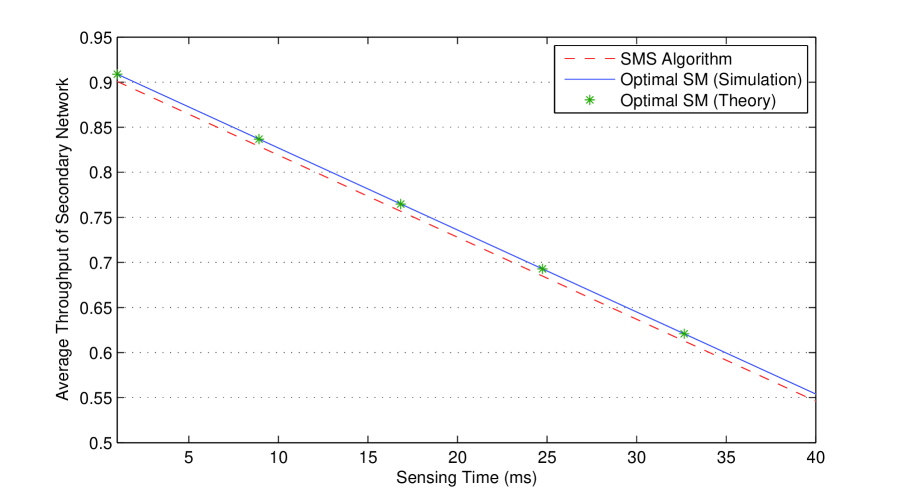
Figure 3: Average throughput versus sensing time for various sensing matrix selection schemes

Fig. 3 validates our analysis and depicts the average throughput (normalized to $R$) of the SUs versus the sensing time, for the optimal SM and the SM obtained based on SMS algorithm, for a error-free sensing case. For the optimal SM, both the theoretical and simulation results are provided. As it can be realized, the throughput linearly decreases by the sensing time. This is due to the fact that for the error-free case, there exists no error in the detection scheme and thus while the increase of sensing time does not have any positive impact on the correct detection, it linearly reduces the transmission time, as can be inferred from (2). Fig. 3 also verifies near-optimality of our proposed algorithm; while it imposes much less complexity burden than the optimum scheme. The relative difference between the average throughput obtained by the SMS algorithm and that obtained by the exhaustive search method is negligible and about $0.81\%$.

Fig. 4 compares the average throughputs of different SUs for a CRN with three SUs, again for a error-free sensing scheme. In this example, it is assumed that the number of primary channels, $N_{p}$, is $5$. The maximum relative difference between the SUs throughputs is $1.84\%$ which confirms the fairness among the SUs when using the proposed scheme. It is expected by running the simulation for more than $100$ times, the difference among the SUs’ throughputs disappears.

Fig. 5 demonstrates the energy efficiency of our proposed algorithm. This Fig. shows the average consumed energy versus the primary user occupation probability. The SUs consumes less average energy to find a transmission opportunity when sensing the channel based on the SM obtained by our proposed method compared to the optimal SM. It is worth noting that in both schemes, the consumed energies of the SUs increase when the PUs’ absence probability decreases; as the SUs have to sense more channels to find free ones.

Fig. 6 compares the average throughputs of various spectrum allocation schemes proposed in this paper. For the two MSMS and PMSMS schemes, a practical scenario with activity detection errors has been assumed. In general, as the sensing time increases, the detector senses the channels more accurately and finds more transmission opportunities. However, by the increase of the sensing time, less time remains for the transmission. Hence, there exist a tradeoff between average throughput and detector accuracy. As it is seen in Fig. 6, first the SUs’ throughput increases by $\tau$ (due to an accurate sensing); then after an optimum point, where $P_{md}$ and $P_{fa}$ are in acceptable levels, the throughput starts decreasing due to the reduction of the time left for the transmission. For a sensing time greater than a specific amount (optimum value), the false alarm and miss-detection probabilities of the detector becomes negligible, and the allocation procedure of the MSMS algorithm as well as its performance will be similar to those of the SMS algorithm, for which a error-free sensing has been assumed. In the MSMS scheme, the SUs sense channels with the probability of $\left(1-P_{fa}\right)$, and thus some transmission opportunities are lost as a result of false alarm. This is the reason that the average throughput of the SUs obtained by the MSMS algorithm is less than that of the SMS algorithm in which $P_{fa}$ is assumed to be zero. In the PMSMS algorithm, the applied p-persistent MAC protocol leads to loss transmission opportunities, and thus to less average throughput compared to the MSMS when the number of SUs is not too high.

Fig. 7 demonstrates the advantages of the exploited PMAC for the case that the number of primary channels are less than the number of SUs. This Fig. shows the average SUs’ throughput versus the probability of sensing an assigned channel (i.e., $p$ in MAC protocol). Note that the performance for $p=1$ is the same as that of the MSMS. As can be realized, for $N_{s}=8$ and $N_{P}=5$, the exploited PMAC protocol can increase the chance of transmission on the channels by reducing the contention level among the SUs. Therefore, the PMSMS scheme can offer higher throughput for the CRN than the MSMS scheme provided that the coordinator appropriately selects the value of $p$, which for the example considered it must be larger than $0.165$. Interestingly, for $p=0.46$, the improvement in the throughput when using the PMSMS scheme is about $48.8\%$ compared to the MSMS scheme.

VIII Conclusion

In this paper, the average throughput of a cognitive radio network (CRN) for a given sensing matrix (SM) has been derived, and an optimization problem has been formulated to find the optimal SM. In order to mitigate the challenges associated with the optimal solution, three novel centralized suboptimal algorithms have been proposed. More specifically, the SMS and MSMS schemes are proposed for error-free and non-perfect sensing cases, respectively, and then the PMSMS algorithm is developed by applying the conventional p-persistent MAC protocol in the MSMS scheme to strengthen the multiple access capability of the CRN. Besides offering throughput close to the maximum achievable one, the benefits of these proposed schemes are threefold. In addition to comparatively low computational complexities, they provide an acceptable level of fairness among secondary users. Further, they offer lower consumed energies compared to the optimum solution. The performance of the proposed schemes has been evaluated, and their efficiencies have been demonstrated through theoretical analysis as well as exhaustive simulation results.

TABLE I: Simulation Parameters

Parameter	Description	Value
$P_{d}^{\min}$	Minimum allowable detection probability	0.9
$P_{fa}^{\max}$	Maximum allowable false alarm probability	0.1
$f_{s}$	Receiver sampling frequency	6 MHz
$T$	Time-slot duration	200 ms
$\tau_{ho}$	Required time for handover	0.1 ms
$N_{p}$	Number of primary users	5
$N_{s}$	Number of primary users	3

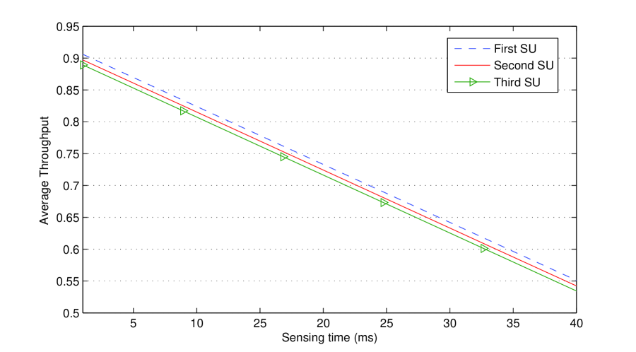
Figure 4: Average throughput versus sensing time for different secondary users

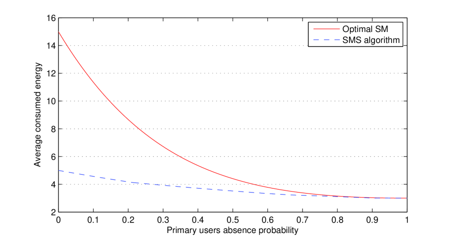
Figure 5: Average consumed energy versus the primary user absence probability

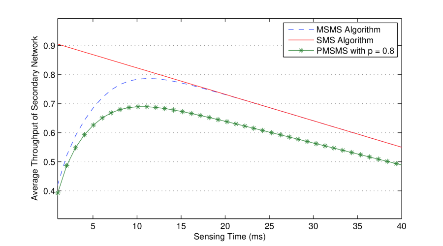
Figure 6: Average throughput of SUs versus sensing time for various proposed schemes.

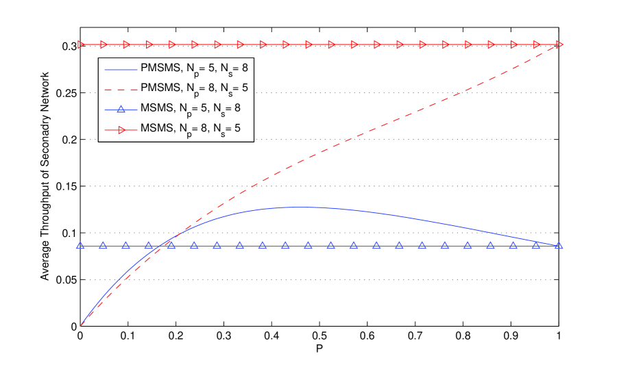
Figure 7: Advantages of exploiting PMAC.

References

- [1] C. Clancy, J. Hecker, E. Stuntebeck, and T. O Shea, “Applications of machine learning to cognitive radio networks,” IEEE Wireless. Commun., vol. 14, no. 4, pp. 47–52, August 2007.
- [2] P. Paysarvi-Hoseini and N. C. Beaulieu, “Optimal wideband spectrum sensing framework for cognitive radio systems,” accepted for publication on IEEE Trans. Signal Process., vol. 47, no. 1, pp. 130–138, Jan 2009.
- [3] Q. Zhao, L. Tong, A. Swami, and Y. Chen, ““decentralized cognitive mac for opportunistic spectrum access in ad hoc networks: A pomdp framework,” IEEE J. on Sel. Areas in Commun., vol. 25, no. 3, pp. 589–600, April 2007.
- [4] L. C. Wang, C. W. Wang, and F. Adachi, “Load-balancing spectrum decision for cognitive radio networks,” IEEE J. on Sel. Areas in Commun., vol. 29, no. 4, April 2011.
- [5] H. J. Liu, S. F. Li, Z. X. Wang, W. J. Hong, and M. Yi, “Strategy of dynamic spectrum access based-on spectrum pool,” IEEE International Conference on Wireless Communications, Networking and Mobile Computing (WiCOM), September 2008.
- [6] A. W. Min and K. G. Shin, “Exploiting multi-channel diversity in spectrum-agile networks,” IEEE International Conference on Computer Communications (INFOCOM), April 2008.
- [7] B. Hamdaoui, “Adaptive spectrum assessment for opportunistic access in cognitive radio networks,” IEEE Trans. Wireless Commun., vol. 8, no. 2, pp. 922–930, February 2009.
- [8] L. Lai, H. E. Gamal, H. Jiang, and H. V. Poor, “Optimal medium access control in cognitive radios: A sequential design approach,” IEEE ICASSP, pp. 2073–2076, March 2008.
- [9] A. Sabharwal, A. Khoshnevis, and E. Knightly, “Opportunistic spectral usage: Bounds and a multi-band csma/ca protocol,” IEEE/ACM Trans. Netw., vol. 15, no. 3, pp. 533–545, June 2007.
- [10] J. Jia, Q. Zhang, and X. S. Shen, ““hc-mac: A hardware-constrained cognitive mac for efficient spectrum management,” IEEE J. Sel. Areas Commun., vol. 26, no. 1, pp. 106–117, June 2008.
- [11] N. B. Chang and M. Liu, “Optimal channel probing and transmission scheduling for opportunistic spectrum access,” in Proc. 13th ACM Annu. Int. Conf. MobiCom, pp. 27–38, Sep. 2007.
- [12] Y. S. Chow, H. Robbins, and D. Siegmund, Great Expectations: The Theory of Optimal Stopping. Boston: Houghton Mifflin, 1971.
- [13] D. Zheng, W. Ge, and J. Zhang, “Distributed opportunistic scheduling for ad-hoc networks with random access: An optimal stopping approach,” IEEE Trans. Inf. Theory, vol. 55, no. 1, pp. 205–222, January 2009.
- [14] H. Kim and K. G. Shin, “Fast discovery of spectrum opportunities in cognitive radio networks,” IEEE DySPAN, October 2008.
- [15] ——, “Efficient discovery of spectrum opportunities with mac-layer sensing in cognitive radio networks,” IEEE Trans. Wireless Commun., vol. 7, no. 5, pp. 533–545, May 2008.
- [16] H. Jiang, L. Lai, R. Fan, and H. V. Poor, “Optimal selection of channel sensing order in cognitive radio,” IEEE Trans. Wireless Commun., vol. 8, no. 1, pp. 297–307, January 2009.
- [17] R. Fan and H. Jiang, “Channel sensing-order setting in cognitive radio networks: A two-user case,” IEEE Trans. Veh. Technol., vol. 58, no. 9, pp. 4997–5008, November 2009.
- [18] Y. C. Liang, Y. Zeng, E. C. Y. Peh, and A. T. Hoang, “Sensing-throughput tradeoff for cognitive radio networks,” IEEE Trans. Wireless Communication, vol. 7, no. 4, pp. 1326–1337, Apr. 2008.
- [19] C. R. Stevenson, G. Chouinard, W. H. Z. Lei, and S. J. Shellhammer, “IEEE 802.22: The first cognitive radio wireless regional area network standard,” IEEE Comm. Mag., vol. 47, no. 1, pp. 130–138, Jan 2009.