Non-Asymptotic Analysis of Tangent Space Perturbation

Abstract

Constructing an efficient parameterization of a large, noisy data set of points lying close to a smooth manifold in high dimension remains a fundamental problem. One approach consists in recovering a local parameterization using the local tangent plane. Principal component analysis (PCA) is often the tool of choice, as it returns an optimal basis in the case of noise-free samples from a linear subspace. To process noisy data samples from a nonlinear manifold, PCA must be applied locally, at a scale small enough such that the manifold is approximately linear, but at a scale large enough such that structure may be discerned from noise. Using eigenspace perturbation theory and non-asymptotic random matrix theory, we study the stability of the subspace estimated by PCA as a function of scale, and bound (with high probability) the angle it forms with the true tangent space. By adaptively selecting the scale that minimizes this bound, our analysis reveals an appropriate scale for local tangent plane recovery. We also introduce a geometric uncertainty principle quantifying the limits of noise-curvature perturbation for stable recovery. With the purpose of providing perturbation bounds that can be used in practice, we propose plug-in estimates that make it possible to directly apply the theoretical results to real data sets. manifold-valued data, tangent space, principal component analysis, subspace perturbation, local linear models, curvature, noise.
2000 Math Subject Classification: 62H25, 15A42, 60B20

1 Introduction and Overview of the Main Results

1.1 Local Tangent Space Recovery: Motivation and Goals

Large data sets of points in high-dimension often lie close to a smooth low-dimensional manifold. A fundamental problem in processing such data sets is the construction of an efficient parameterization that allows for the data to be well represented in fewer dimensions. Such a parameterization may be realized by exploiting the inherent manifold structure of the data. However, discovering the geometry of an underlying manifold from only noisy samples remains an open topic of research.

The case of data sampled from a linear subspace is well studied (see Johnstone ; Jung-Marron ; Nadler , for example). The optimal parameterization is given by principal component analysis (PCA), as the singular value decomposition (SVD) produces the best low-rank approximation for such data. However, most interesting manifold-valued data organize on or near a nonlinear manifold. PCA, by projecting data points onto the linear subspace of best fit, is not optimal in this case as curvature may only be accommodated by choosing a subspace of dimension higher than that of the manifold. Algorithms designed to process nonlinear data sets typically proceed in one of two directions. One approach is to consider the data globally and produce a nonlinear embedding. Alternatively, the data may be considered in a piecewise-linear fashion and linear methods such as PCA may be applied locally. The latter is the subject of this work.

Local linear parameterization of manifold-valued data requires the estimation of the local tangent space (“tangent plane”) from a neighborhood of points. However, sample points are often corrupted by high-dimensional noise and any local neighborhood deviates from the linear assumptions of PCA due to the curvature of the manifold. Therefore, the subspace recovered by local PCA is a perturbed version of the true tangent space. The goal of the present work is to characterize the stability and accuracy of local tangent space estimation using eigenspace perturbation theory.

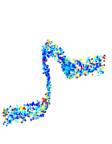
(a) small neighborhoods

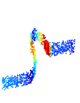
(b) large neighborhoods

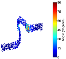
(c) adaptive neighborhoods

Figure 1: Angle between estimated and true tangent planes at each point of a noisy 2-dimensional data set embedded in $\operatorname{\mathbb{R}}^{3}$. The estimated tangent planes are (a) randomly oriented when computed from small neighborhoods within the noise; (b) misaligned when computed from large neighborhoods exhibiting curvature; and (c) properly oriented when computed from adaptively defined neighborhoods given by the analysis in this work.

The proper neighborhood for local tangent space recovery must be a function of intrinsic (manifold) dimension, curvature, and noise level; these properties often vary as different regions of the manifold are explored. However, local PCA approaches proposed in the data analysis and manifold learning literature often define locality via an a priori fixed number of neighbors or as the output of clustering and partitioning algorithms (e.g., LLE ; Zhang-Zha ; Kam-Leen ; Yang ). Other methods Brand ; Ohtake ; Lin-Tong adaptively estimate local neighborhood size but are not tuned to the perturbation of the recovered subspace. Our approach studies this perturbation as the size of the neighborhood varies to guide the definition of locality. On the one hand, a neighborhood must be small enough so that it is approximately linear and avoids curvature. On the other hand, a neighborhood must be be large enough to overcome the effects of noise. A simple yet instructive example of these competing criteria is shown in Figure 1. The tangent plane at every point of a noisy 2-dimensional data set embedded in $\operatorname{\mathbb{R}}^{3}$ is computed via local PCA. Each point is color coded according to the angle formed with the true tangent plane. Three different neighborhood definitions are used: a small, fixed radius (Figure 1a); a large, fixed radius (Figure 1b); and radii defined adaptively according to the analysis presented in this work (Figure 1c). As small neighborhoods may be within the noise level and large neighborhoods exhibit curvature, the figure shows that neither allows for accurate tangent plane recovery. In fact, because the curvature varies across the data, only the adaptively defined neighborhoods avoid random orientation due to noise (as seen in Figure 1a) and misalignment due to curvature (as seen in Figure 1b). Figure 1c shows accurate and stable recovery at almost every data point, with misalignment only in the small region of very high curvature that will be troublesome for any method. The present work quantifies this observed behavior in the high-dimensional setting.

We present a non-asymptotic, eigenspace perturbation analysis to bound, with high probability, the angle between the recovered linear subspace and the true tangent space as the size of the local neighborhood varies. The analysis accurately tracks the subspace recovery error as a function of neighborhood size, noise, and curvature. Thus, we are able to adaptively select the neighborhood that minimizes this bound, yielding the best estimate to the local tangent space from a large but finite number of noisy manifold samples. Further, the behavior of this bound demonstrates the non-trivial existence of such an optimal scale. We also introduce a geometric uncertainty principle quantifying the limits of noise-curvature perturbation for tangent space recovery.

An important technical matter that one needs to address when analyzing points that are sampled from a manifold blurred with Gaussian noise concerns the probability distribution of the noisy samples. Indeed, after perturbation with Gaussian noise, the probability density function of the noisy points can be expressed as the convolution of the probability density function of the clean points on the manifold with a Gaussian kernel. Geometrically, the points are diffused into a tube around the manifold, and the corresponding density of the points is thinned. This concept has been studied in great detail in Maggioni-MIT ; LittleThesisDuke as well as in Niyogi11 ; Genovese12b . The practical implication of these studies is that concentration of measure helps us to guarantee that the volume of noisy points in a ball centered on the clean manifold can be estimated from the volume of the corresponding ball of clean points, provided one applies a correction of the radius. We take advantage of these ideas in our analysis by replacing the ball of noisy points in the tube with a ball of similar volume extracted from the clean manifold, perturbed by Gaussian noise. We introduce the resulting, necessary modification to the radii in Section 5. A related issue concerns the determination of the point $x_{0}$ about which we estimate the tangent plane. From a practical perspective, one can only observe noisy samples, and it is therefore reasonable that the perturbation bound should account for the fact that the analysis cannot be centered around the clean manifold. The expected effect of this additional source of uncertainty has been explored in detail in Maggioni-MIT ; LittleThesisDuke . In this paper, we propose a different approach. We devise a plug-in method to estimate a clean point $x_{0}$ on the manifold using the observed noisy data. As a result, the theoretical analysis can proceed assuming that $x_{0}$ is given by an oracle. Our experiments confirm that the local origin $x_{0}$ on the manifold can be estimated from the noisy neighborhood of observed points and that the perturbation error can be accurately tracked in practice. In addition, we expect this novel denoising algorithm to provide a universal tool for the analysis of noisy point cloud data.

Our analysis is related to the very recent work of Tyagi, et al. Tyagi , in which neighborhood size and sampling density conditions are given to ensure a small angle between the PCA subspace and the true tangent space of a noise-free manifold. Results are extended to arbitrary smooth embeddings of the manifold model, which we do not consider. In contrast, we envision the scenario in which no control is given over the sampling and explore the case of data sampled according to a fixed density and corrupted by high-dimensional noise. Crucial to our results is a careful analysis of the interplay between the perturbation due to noise and the perturbation due to curvature. Nonetheless, our results can be shown to recover those of Tyagi in the noise-free setting. Our approach is also similar to the analysis presented by Nadler in Nadler , who studies the finite-sample properties of the PCA spectrum. Through matrix perturbation theory, Nadler examines the angle between the leading finite-sample-PCA eigenvector and that of the leading population-PCA eigenvector. As a linear model is assumed, perturbation results from noise only. Despite this difference, the two analyses utilize similar techniques to bound the effects of perturbation on the PCA subspace and our results recover those of Nadler in the curvature-free setting.

Application of multiscale PCA for geometric analysis of data sets has also been studied in Fukunaga-Olsen ; Froehling ; Wang-Marron ; Broomhead . In parallel to our work Kaslovsky11a ; Kaslovsky11b ; Meyer12b ; Kaslovsky12a , Maggioni and coauthors have developed results LittleThesisDuke ; Maggioni-long ; Maggioni-MIT addressing similar questions as those examined in this paper. These results are discussed above as well as in more detail in Section 5 and Section 6. Other recent related works include that of Singer and Wu Singer , who use local PCA to build a tangent plane basis and give an analysis for the neighborhood size to be used in the absence of noise. Using the hybrid linear model, Zhang, et al. Lerman assume data are samples from a collection of “flats” (affine subspaces) and choose an optimal neighborhood size from which to recover each flat by studying the least squares approximation error in the form of Jones’ $\beta$-number (see Jones and also Jones-new in which this idea is used for curve denoising). Finally, an analysis of noise and curvature for normal estimation of smooth curves and surfaces in $\mathbb{R}^{2}$ and $\mathbb{R}^{3}$ is presented by Mitra, et al. Guibas-normal-estimation with application to computer graphics.

1.2 Overview of the Results

We consider the problem of recovering the best approximation to a local tangent space of a nonlinear $d$-dimensional Riemannian manifold $\mathcal{M}$ from noisy samples presented in dimension $D>d$. Working about a reference point $x_{0}$, an approximation to the tangent space of $\mathcal{M}$ at $x_{0}$ is given by the span of the top $d$ eigenvectors of the centered data covariance matrix (where “top” refers to the $d$ eigenvectors or singular vectors associated with the $d$ largest eigenvalues or singular values). The question becomes: how many neighbors of $x_{0}$ should be used (or in how large of a radius about $x_{0}$ should we work) to recover the best approximation? We will often use the term “scale” to refer to this neighborhood size or radius.

To answer this question, we consider the perturbation of the eigenvectors spanning the estimated tangent space in the context of the “noise-curvature trade-off.” To balance the effects of noise and curvature (as observed in the example of the previous subsection, Figure 1), we seek a scale large enough to be above the noise level but still small enough to avoid curvature. This scale reveals a linear structure that is sufficiently decoupled from both the noise and the curvature to be well approximated by a tangent plane. At this scale, the recovered eigenvectors span a subspace corresponding very closely to the true tangent space of the manifold at $x_{0}$. We note that the concept of noise-curvature trade-off has been a subject of interest for decades in dynamical systems theory Froehling .

The main result of this work is a bound on the angle between the computed and true tangent spaces. Define $P$ to be the orthogonal projector onto the true tangent space and let $\widehat{P}$ be the orthogonal projector constructed from the $d$-dimensional eigenspace of the neighborhood covariance matrix. Then the distance $\|P-\widehat{P}\|_{F}^{2}$ corresponds to the sum of the squared sines of the principal angles between the computed and true tangent spaces and we use eigenspace perturbation theory to bound this norm. Momentarily neglecting probability-dependent constants to ease the presentation, the first-order approximation of this bound has the following form:

Informal Main Result.

$${\color[rgb]{0,0,0}\|P-\widehat{P}\|_{F}~{}\leq~{}\frac{\frac{2\sqrt{2}}{\sqrt{N}}\left[K^{(+)}r^{3}+\sigma\sqrt{d(D-d)}\left(\sigma+\frac{r}{\sqrt{d+2}}+\frac{\mathcal{K}^{1/2}r^{2}}{(d+2)\sqrt{2(d+4)}}\right)\right]}{\frac{r^{2}}{d+2}-\frac{\mathcal{K}r^{4}}{2(d+2)^{2}(d+4)}-\sigma^{2}\left(\sqrt{d}+\sqrt{D-d}\right)},}$$ (1)

where $r$ is the radius (measured in the tangent plane) of the neighborhood containing $N$ points, $\sigma$ is the noise level, and $K^{(+)}$ and $\mathcal{K}$ are functions of curvature.
To aid the interpretation, we note that $K^{(+)}$ corresponds to the Frobenius norm of the matrix of principal curvatures and $\mathcal{K}$ has size $2d(D-d)\kappa^{2}$ in the case where all principal curvatures are equal to $\kappa$. The quantities $N$, $r$, $\sigma$, $K^{(+)}$, and $\mathcal{K}$, as well as the sampling assumptions are more formally defined in Sections 2 and 3, and the formal result is presented in Section 3.

The denominator of this bound, denoted here by $\delta_{\text{informal}}$,

$${\color[rgb]{0,0,0}\delta_{\text{informal}}=\frac{r^{2}}{d+2}-\frac{\mathcal{K}r^{4}}{2(d+2)^{2}(d+4)}-\sigma^{2}\left(\sqrt{d}+\sqrt{D-d}\right)}$$ (2)

quantifies the separation between the spectrum of the linear subspace ($\approx r^{2}$) and the perturbation due to curvature ($\approx\mathcal{K}r^{4}$) and noise ($\approx\sigma^{2}(\sqrt{d}+\sqrt{D-d})$). Clearly, we must have $\delta_{\text{informal}}>0$ to approximate the appropriate linear subspace, a requirement made formal by Theorem 3.2 in Section 3. In general, when $\delta_{\text{informal}}$ is zero (or negative), the bound becomes infinite (or negative) and is not useful for subspace recovery. However, the geometric information encoded by (1) offers more insight. For example, we observe that a small $\delta_{\text{informal}}$ indicates that the estimated subspace contains a direction orthogonal to the true tangent space (due to the curvature or noise). We therefore consider $\delta_{\text{informal}}$ to be the condition number for subspace recovery and use it to develop our geometric interpretation for the bound.

The noise-curvature trade-off is readily apparent from (1). The linear and curvature contributions are small for small values of $r$. Thus for a small neighborhood ($r$ small), the denominator (2) is either negative or ill conditioned for most values of $\sigma$ and the bound becomes large. This matches our intuition as we have not yet encountered much curvature but the linear structure has also not been explored. Therefore, the noise dominates the early behavior of this bound and an approximating subspace may not be recovered from noise. As the neighborhood radius $r$ increases, the conditioning of the denominator improves, and the bound is controlled by the $1/\sqrt{N}$ behavior of the numerator. This again corresponds with our intuition: the addition of more points serves to overcome the effects of noise as the linear structure is explored. Thus, when $\delta_{\text{informal}}^{-1}$ is well conditioned, the bound on the angle may become smaller with the inclusion of more points. Eventually $r$ becomes large enough such that the curvature contribution approaches the size of the linear contribution and $\delta_{\text{informal}}^{-1}$ becomes large. The $1/\sqrt{N}$ term is overtaken by the ill conditioning of the denominator and the bound is again forced to become large. The noise-curvature trade-off, seen analytically here in (1) and (2), will be demonstrated numerically in Section 4.

Enforcing a well conditioned recovery bound (1) yields a geometric uncertainty principle quantifying the amount of curvature and noise we may tolerate. To recover an approximating subspace, we must have:

Geometric Uncertainty Principle.

$${\color[rgb]{0,0,0}\mathcal{K}\sigma^{2}~{}<~{}\frac{d+4}{2(\sqrt{d}+\sqrt{D-d})}}$$ (3)

By preventing the curvature and noise level from simultaneously becoming large, this requirement ensures that the linear structure of the data is recoverable. With high probability, the noise component normal to the tangent plane concentrates on a sphere with mean curvature $1/(\sigma\sqrt{D-d})$. As will be shown, this uncertainty principle expresses the intuitive notion that the curvature of the manifold must be less than the curvature of this noise-ball. Otherwise, the combined effects of noise and curvature perturbation prevent an accurate estimate of the local tangent space.

We note that the concept of a geometric uncertainty principle also appears in the context of the computation of the homology of the manifold $\mathcal{M}$ in Niyogi11 . As explained in detail in Section 3.2, the two principles are strikingly similar.

The remainder of the paper is organized as follows. Section 2 provides the notation, geometric model, and necessary mathematical formulations used throughout this work. Eigenspace perturbation theory is reviewed in this section. The main results are stated formally in Section 3. We demonstrate the accuracy of our results and test the sensitivity to errors in parameter estimation in Section 4. Section 5 presents the modifications that are needed to account for the sampling density of the noisy points, and introduces two plug-in estimates that can be used in practice to apply the theoretical results of Section 3 to a real data set. We conclude in Section 6 with a discussion of the relationship to previously established results and further algorithmic considerations. Technical results and proofs are presented in the appendices.

2 Mathematical Preliminaries

2.1 Geometric Data Model

A $d$-dimensional Riemannian manifold of codimension 1 may be described locally about a reference point $x_{0}$ by the surface $y=f(\ell_{1},\dots,\ell_{d})$, where $\ell_{i}$ is a coordinate in the tangent plane, ${T_{x_{0}}\negthinspace\mathcal{M}}$, to the manifold at $x_{0}$. After translating $x_{0}$ to the origin, we have

$$x_{0}=[0~{}0~{}\cdots~{}0]^{T},$$

and a rotation of the coordinate system can align the coordinate axes with the principal directions associated with the principal curvatures at $x_{0}$. Aligning the coordinate axes with the plane tangent to $\mathcal{M}$ at $x_{0}$ gives a local quadratic approximation to the manifold. Using this choice of coordinates, the manifold may be described locally Giaquinta by the Taylor series of $f$ at $x_{0}$:

$$y=f(\ell_{1},\dots,\ell_{d})=\frac{1}{2}(\kappa_{1}\ell_{1}^{2}+\dots+\kappa_{d}\ell_{d}^{2})+o\left(\ell_{1}^{2}+\dots+\ell_{d}^{2}\right),$$ (4)

where $\kappa_{1},\dots,\kappa_{d}$ are the principal curvatures of $\mathcal{M}$ at $x_{0}$. In this coordinate system, a point $x$ in a neighborhood of $x_{0}$ has the form

$$x=[\ell_{1}~{}\ell_{2}~{}\cdots~{}\ell_{d}~{}f(\ell_{1},\dots,\ell_{d})]^{T}.$$

Generalizing to a $d$-dimensional manifold of arbitrary codimension in $\mathbb{R}^{D}$, there exist $(D-d)$ functions

$$f_{i}(\ell)=\frac{1}{2}(\kappa^{(i)}_{1}\ell_{1}^{2}+\dots+\kappa^{(i)}_{d}\ell_{d}^{2})+o\left(\ell_{1}^{2}+\dots+\ell_{d}^{2}\right),$$ (5)

for $i=(d+1),\dots,D$, with $\kappa^{(i)}_{1},\dots,\kappa^{(i)}_{d}$ representing the principal curvatures in the $i$th normal direction at $x_{0}$. Then, given the coordinate system aligned with the principal directions, a point in a neighborhood of $x_{0}$ has coordinates $\left[\ell_{1},\dots,\ell_{d},f_{d+1},\dots,f_{D}\right]$. We truncate the Taylor expansion (5) and use the quadratic approximation

$$f_{i}(\ell)=\frac{1}{2}(\kappa^{(i)}_{1}\ell_{1}^{2}+\dots+\kappa^{(i)}_{d}\ell_{d}^{2}),$$ (6)

$i=(d+1),\dots,D$, to describe the manifold locally.

Consider now discrete samples from $\mathcal{M}$ obtained by uniformly sampling the first $d$ coordinates ($\ell_{1},\dots,\ell_{d})$ in the tangent space inside $B^{d}_{x_{0}}(r)$, the $d$-dimensional ball of radius $r$ centered at $x_{0}$, with the remaining $(D-d)$ coordinates given by (6). Because we are sampling from a noise-free linear subspace, the number of points $N$ captured inside $B^{d}_{x_{0}}(r)$ is a function of the sampling density $\rho$:

$$N=\rho v_{d}r^{d},$$ (7)

where $v_{d}$ is the volume of the $d$-dimensional unit ball. The sampled points are assumed to be in general linear position, a standard assumption when sampling from a linear subspace (see Remark 2.3).

Finally, we assume the sample points of $\mathcal{M}$ are contaminated with an additive Gaussian noise vector $e$ drawn from the $\operatorname{\mathcal{N}}\left(0,\sigma^{2}I_{D}\right)$ distribution. Each sample $x$ is a $D$-dimensional vector, and $N$ such samples may be stored as columns of a matrix $X\in\mathbb{R}^{D\times N}$. The coordinate system above allows the decomposition of $x$ into its linear (tangent plane) component $\ell$, its quadratic (curvature) component $c$, and noise $e$, three $D$-dimensional vectors

$$\ell =[\ell_{1}~{}\ell_{2}~{}\cdots~{}~{}\ell_{d}~{}~{}0~{}~{}~{}\cdots~{}~{}~{}0]^{T}$$ (8)

$$c =[0~{}~{}~{}~{}\cdots~{}~{}~{}~{}0~{}c_{d+1}~{}\cdots~{}c_{D}]^{T}$$ (9)

$$e =[e_{1}~{}e_{2}~{}\quad\quad\;\;\cdots\quad\quad\;\;e_{D}]^{T}$$ (10)

such that the last $(D-d)$ entries of $c$ are of the form $c_{i}=f_{i}(\ell)$, $i=(d+1),\dots,D$. We may store the $N$ samples of $\ell$, $c$, and $e$ as columns of matrices $L$, $C$, $E$, respectively, such that our data matrix is decomposed as

$$X=L+C+E.$$ (11)

The true tangent space we wish to recover is given by the PCA of $L$. Because we do not have direct access to $L$, we work with $X$ as a proxy, and instead recover a subspace spanned by the corresponding eigenvectors of $XX^{T}$. We will study how close this recovered invariant subspace of $XX^{T}$ is to the corresponding invariant subspace of $LL^{T}$ as a function of scale. Throughout this work, scale refers to the number of points $N$ in the local neighborhood within which we perform PCA. Given a fixed density of points, scale may be equivalently quantified as the radius $r$ about the reference point $x_{0}$ defining the local neighborhood.

Remark 2.1.

Of course it is unrealistic for the data to be observed in the described coordinate system. As noted, we may use a rotation to align the coordinate axes with the principal directions associated with the principal curvatures. Doing so allows us to write (6) as well as (11). Because we will ultimately quantify the norm of each matrix using the unitarily-invariant Frobenius norm, this rotation will not affect our analysis. We therefore proceed by assuming that the coordinate axes align with the principal directions.

Remark 2.2.

Equation (6) represents an exact quadratic embedding of $\mathcal{M}$. While it may be interesting to consider more general embeddings, as is done for the noise-free case in Tyagi , a Taylor expansion followed by rotation and translation will result in an embedding of the form (5). Noting that the numerical results of Tyagi indicate no loss in accuracy when truncating higher-order terms, proceeding with an analysis of (6) remains sufficiently general.

Remark 2.3.

In a non-pathological configuration (e.g., points observed in general linear position), only $d+1$ sample points are needed to ensure that the top $d$ eigenvectors of $LL^{T}$ span the true tangent space. It has been noted in the literature (e.g., Rudelson-Isotropic ; Vershynin-HowClose ) that $\mathcal{O}(d\log d)$ points should be sampled for the empirical covariance matrix to be close in norm to the population covariance, with high probability. Strictly enforcing this sampling condition is a very mild requirement for our setting, in which the sampling density $\rho$ (see equation (7)) is usually large and the extra logarithmic factor of $d$ is easily achieved. Further, this logarithmic factor is implicitly present in our analysis as a consequence of the lower bound on the smallest eigenvalue of $LL^{T}$ (see Appendix A.1). We also note that we do not intend to analyze the extremely small scales (very small $N$) where finite sample effects create instability and prevent a meaningful analysis.

2.2 Perturbation of Invariant Subspaces

Given the decomposition of the data (11), we have

$$XX^{T}~{}=~{}LL^{T}+CC^{T}+EE^{T}+LC^{T}+CL^{T}+LE^{T}+EL^{T}+CE^{T}+EC^{T}.$$ (12)

We introduce some notation to account for the centering required by PCA. Define the sample mean of $N$ realizations of random vector $m$ as

$$\overline{m}=\frac{1}{N}\sum_{i=1}^{N}m^{(i)},$$ (13)

where $m^{(i)}$ denotes the $i$th realization. Letting $\mathbf{1}_{N}$ represent the column vector of $N$ ones, define

$$\overline{M}=\overline{m}\mathbf{1}_{N}^{T}$$ (14)

to be the matrix with $N$ copies of $\overline{m}$ as its columns. Finally, let $\widetilde{M}$ denote the centered version of $M$:

$$\widetilde{M}~{}=~{}M-\overline{M}.$$ (15)

Then we have

$$\widetilde{X}\widetilde{X}^{T}~{}=~{}\widetilde{L}\widetilde{L}^{T}+\widetilde{C}\widetilde{C}^{T}+\widetilde{E}\widetilde{E}^{T}+\widetilde{L}\widetilde{C}^{T}+\widetilde{C}\widetilde{L}^{T}+\widetilde{L}\widetilde{E}^{T}+\widetilde{E}\widetilde{L}^{T}+\widetilde{C}\widetilde{E}^{T}+\widetilde{E}\widetilde{C}^{T}.$$ (16)

The problem may be posed as a perturbation analysis of invariant subspaces. Rewrite (12) as

$$\frac{1}{N}\widetilde{X}\widetilde{X}^{T}=\frac{1}{N}\widetilde{L}\widetilde{L}^{T}+\Delta,$$ (17)

where

$$\Delta=\frac{1}{N}(\widetilde{C}\widetilde{C}^{T}+\widetilde{E}\widetilde{E}^{T}+\widetilde{L}\widetilde{C}^{T}+\widetilde{C}\widetilde{L}^{T}+\widetilde{L}\widetilde{E}^{T}+\widetilde{E}\widetilde{L}^{T}+\widetilde{C}\widetilde{E}^{T}+\widetilde{E}\widetilde{C}^{T})$$ (18)

is the perturbation that prevents us from working directly with $\widetilde{L}\widetilde{L}^{T}$. The dominant eigenspace of $\widetilde{X}\widetilde{X}^{T}$ is therefore a perturbed version of the dominant eigenspace of $\widetilde{L}\widetilde{L}^{T}$. Seeking to minimize the effect of this perturbation, we look for the scale $N^{*}$ (equivalently $r^{*}$) at which the dominant eigenspace of $\widetilde{X}\widetilde{X}^{T}$ is closest to that of $\widetilde{L}\widetilde{L}^{T}$. Before proceeding, we review material on the perturbation of eigenspaces relevant to our analysis. The reader familiar with this topic is invited to skip directly to Theorem 2.4.

The distance between two subspaces of $\mathbb{R}^{D}$ can be defined as the spectral norm of the difference between their respective orthogonal projectors GVL . As we will always be considering two equidimensional subspaces, this distance is equal to the sine of the largest principal angle between the subspaces. To control all such principal angles, we state our results using the Frobenius norm of this difference. Our goal is therefore to control the behavior of $\|P-\widehat{P}\|_{F}$, where $P$ and $\widehat{P}$ are the orthogonal projectors onto the subspaces computed from $L$ and $X$, respectively.

The norm $\|P-\widehat{P}\|_{F}$ may be bounded by the classic $\sin\Theta$ theorem of Davis and Kahan Davis . We will use a version of this theorem presented by Stewart (Theorem V.2.7 of Stewart ), modified for our specific purpose. First, we establish some notation, following closely that found in Stewart . Consider the eigendecompositions

$$\frac{1}{N}\widetilde{L}\widetilde{L}^{T} =U\Lambda U^{T}=[U_{1}~{}U_{2}]~{}\begin{bmatrix}\Lambda_{1}&\\ &\Lambda_{2}\end{bmatrix}~{}[U_{1}~{}U_{2}]^{T},$$ (19)

$$\frac{1}{N}\widetilde{X}\widetilde{X}^{T} =\widehat{U}\widehat{\Lambda}\widehat{U}^{T}=[\widehat{U}_{1}~{}\widehat{U}_{2}]~{}\begin{bmatrix}\widehat{\Lambda}_{1}&\\ &\widehat{\Lambda}_{2}\end{bmatrix}~{}[\widehat{U}_{1}~{}\widehat{U}_{2}]^{T},$$ (20)

such that the columns of $U$ are the eigenvectors of $\frac{1}{N}\widetilde{L}\widetilde{L}^{T}$ and the columns of $\widehat{U}$ are the eigenvectors of $\frac{1}{N}\widetilde{X}\widetilde{X}^{T}$. The eigenvalues of $\frac{1}{N}\widetilde{L}\widetilde{L}^{T}$ are arranged in descending order as the entries of diagonal matrix $\Lambda$. The eigenvalues are also partitioned such that diagonal matrices $\Lambda_{1}$ and $\Lambda_{2}$ contain the $d$ largest entries of $\Lambda$ and the $(D-d)$ smallest entries of $\Lambda$, respectively. The columns of $U_{1}$ are those eigenvectors associated with the $d$ eigenvalues in $\Lambda_{1}$, the columns of $U_{2}$ are those eigenvectors associated with the $(D-d)$ eigenvalues in $\Lambda_{2}$, and the eigendecomposition of $\frac{1}{N}\widetilde{X}\widetilde{X}^{T}$ is similarly partitioned. The subspace we recover is spanned by the columns of $\widehat{U}_{1}$ and we wish to have this subspace as close as possible to the tangent space spanned by the columns of $U_{1}$. The orthogonal projectors onto the tangent and computed subspaces, $P$ and $\widehat{P}$ respectively, are given by

$$P =U_{1}U_{1}^{T}\quad\text{and}\quad\widehat{P}=\widehat{U}_{1}\widehat{U}_{1}^{T}.$$

Define $\lambda_{d}$ to be the $d$th largest eigenvalue of $\frac{1}{N}\widetilde{L}\widetilde{L}^{T}$, or the last entry on the diagonal of $\Lambda_{1}$. This eigenvalue corresponds to variance in a tangent space direction.

We are now in position to state the theorem. Note that we have made use of the fact that the columns of $U$ are the eigenvectors of $\widetilde{L}\widetilde{L}^{T}$, that $\Lambda_{1},\Lambda_{2}$ are Hermitian (diagonal) matrices, and that the Frobenius norm is used to measure distances. The reader is referred to Stewart for the theorem in its original form.

Theorem 2.4 (Davis & Kahan Davis , Stewart Stewart ).

Let

$$\delta=\lambda_{d}-\left\|U_{1}^{T}\Delta U_{1}\right\|_{F}-\left\|U_{2}^{T}\Delta U_{2}\right\|_{F}$$

and consider

• (Condition 1)  $\delta>0$

• (Condition 2)  $\left\|U_{1}^{T}\Delta U_{2}\right\|_{F}\left\|U_{2}^{T}\Delta U_{1}\right\|_{F}<\frac{1}{4}\delta^{2}$.

Then, provided that conditions 1 and 2 hold,

$$\left\|P-\widehat{P}\right\|_{F}~{}\leq~{}2\sqrt{2}~{}\frac{\left\|U_{2}^{T}\Delta U_{1}\right\|_{F}}{\delta}.\\$$ (21)

It is instructive to consider the perturbation $\Delta$ as an operator with range in $\mathbb{R}^{D}$ and quantify its effect on the existing invariant subspaces. Consider first the idealized case where $U_{1}$ is an invariant subspace of $\Delta$, i.e., $\Delta$ maps points from the column space of $U_{1}$ to the column space of $U_{1}$. Clearly, $U_{2}^{T}\Delta U_{1}=0$ in this case as the subspace spanned by $U_{1}$ remains invariant under the action of $\Delta$, and the perturbation angle is zero. In general, however, we cannot expect such an idealized restriction for the range of $\Delta$ and we therefore expect that $\Delta U_{1}$ will have a component that is normal to the tangent space. The numerator $\|U_{2}^{T}\Delta U_{1}\|_{F}$ of (21) measures this normal component, thereby quantifying the effect of the perturbation on the tangent space. Then $\|U_{1}^{T}\Delta U_{1}\|_{F}$ measures the component that remains in the tangent space after the action of $\Delta$. As this component does not contain curvature, $\|U_{1}^{T}\Delta U_{1}\|_{F}$ corresponds to the spectrum of the noise projected in the tangent space. Similarly, $\|U_{2}^{T}\Delta U_{2}\|_{F}$ measures the spectrum of the curvature and noise perturbation normal to the tangent space. Thus, when $\Delta$ leaves the column space of $U_{1}$ mostly unperturbed (i.e., $\|U_{2}^{T}\Delta U_{1}\|_{F}$ is small) and the spectrum of the tangent space is well separated from that of the noise and curvature, the estimated subspace will form only a small angle with the true tangent space. In the next section, we use the machinery of this classic result to bound the angle caused by the perturbation $\Delta$ and develop an interpretation of the conditions of Theorem 2.4 suited to the noise-curvature trade-off.

3 Main Results

Given the framework for analysis developed above, the terms appearing in the statement of Theorem 2.4 ($\left\|U_{1}^{T}\Delta U_{1}\right\|_{F}$, $\left\|U_{2}^{T}\Delta U_{2}\right\|_{F}$, $\left\|U_{2}^{T}\Delta U_{1}\right\|_{F}$, $\left\|U_{1}^{T}\Delta U_{2}\right\|_{F}$, and $\lambda_{d}$) must be controlled. We notice that $\Delta$ is a symmetric matrix, so that $\left\|U_{1}^{T}\Delta U_{2}\right\|_{F}=\left\|U_{2}^{T}\Delta U_{1}\right\|_{F}$. Using the triangle inequality and the geometric constraints

$$U_{1}^{T}C=0\quad\text{and}\quad U_{2}^{T}L=0,$$ (22)

the norms may be controlled by bounding the contribution of each term in the perturbation $\Delta$:

$$\left\|U_{1}^{T}\Delta U_{1}\right\|_{F} \leq 2\left\|U_{1}^{T}\frac{1}{N}\widetilde{L}\widetilde{E}^{T}U_{1}\right\|_{F}+\;\;\,\left\|U_{1}^{T}\frac{1}{N}\widetilde{E}\widetilde{E}^{T}U_{1}\right\|_{F},$$

$$\left\|U_{2}^{T}\Delta U_{2}\right\|_{F} \leq\;\;\,\left\|U_{2}^{T}\frac{1}{N}\widetilde{C}\widetilde{C}^{T}U_{2}\right\|_{F}+2\left\|U_{2}^{T}\frac{1}{N}\widetilde{C}\widetilde{E}^{T}U_{2}\right\|_{F}+\left\|U_{2}^{T}\frac{1}{N}\widetilde{E}\widetilde{E}^{T}U_{2}\right\|_{F},$$

$$\left\|U_{2}^{T}\Delta U_{1}\right\|_{F} \leq\;\;\,\left\|U_{2}^{T}\frac{1}{N}\widetilde{C}\widetilde{L}^{T}U_{1}\right\|_{F}+\;\;\,\left\|U_{2}^{T}\frac{1}{N}\widetilde{E}\widetilde{L}^{T}U_{1}\right\|_{F}+\,\left\|U_{2}^{T}\frac{1}{N}\widetilde{C}\widetilde{E}^{T}U_{1}\right\|_{F}+\,\left\|U_{2}^{T}\frac{1}{N}\widetilde{E}\widetilde{E}^{T}U_{1}\right\|_{F}.$$

Importantly, we seek control over each (right-hand side) term in the finite-sample regime, as we assume a possibly large but finite number of sample points $N$. Therefore, bounds are derived through a careful analysis employing concentration results and techniques from non-asymptotic random matrix theory. The technical analysis is presented in the appendix and proceeds by analyzing three distinct cases: the covariance of bounded random matrices, unbounded random matrices, and the interaction of bounded and unbounded random matrices. The eigenvalue $\lambda_{d}$ is bounded again using random matrix theory. In all cases, care is taken to ensure that bounds hold with high probability that is independent of the ambient dimension $D$.

Remark 3.1.

Other, possibly tighter, avenues of analysis may be possible for some of the bounds presented in the appendix. However, the presented analysis avoids large union bounds and dependence on the ambient dimension to state results holding with high probability. Alternative analyses are possible, often sacrificing probability to exhibit sharper concentration. We proceed with a theoretical analysis holding with the highest probability while maintaining accurate results.

3.1 Bounding the Angle Between Subspaces

We are now in position to apply Theorem 2.4 and state our main result. First, we make the following definitions involving the principal curvatures:

$$K_{i}=\sum_{n=1}^{d}\kappa_{n}^{(i)},\quad K=\left(\sum_{i=d+1}^{D}K_{i}^{2}\right)^{\frac{1}{2}},$$ (23)

$$K_{nn}^{ij}=\sum_{n=1}^{d}\kappa_{n}^{(i)}\kappa_{n}^{(j)},\quad K_{mn}^{ij}=\sum_{\begin{subarray}{c}m,n=1\\ m\neq n\end{subarray}}^{d}\kappa_{m}^{(i)}\kappa_{n}^{(j)},$$ (24)

and

$${\color[rgb]{0,0,0}\mathcal{K}=\left[\sum_{i=d+1}^{D}\sum_{j=d+1}^{D}\left[(d+1)K_{nn}^{ij}-K_{mn}^{ij}\right]^{2}\right]^{\frac{1}{2}}.}$$ (25)

The constant $K_{i}$ is the mean curvature (rescaled by a factor of $d$) in normal direction $i$, for $(d+1)\leq i\leq D$. The curvature of the local model is quantified by $K$, which is a natural result of our use of the Frobenius norm, and $\mathcal{K}$, which results from the expectation of the norm of the curvature covariance. Note that $K_{i}K_{j}=K_{nn}^{ij}+K_{mn}^{ij}$. We also define the constants

$$K_{i}^{(+)}=\left(\sum_{n=1}^{d}|\kappa_{n}^{(i)}|^{2}\right)^{\frac{1}{2}},\quad\text{and}\quad K^{(+)}=\left(\sum_{i=d+1}^{D}(K_{i}^{(+)})^{2}\right)^{\frac{1}{2}}$$ (26)

to be used when strictly positive curvature terms are required.

The main result is formulated in the appendix and makes the following benign assumptions on the number of sample points $N$ and the probability constants $\xi$ and $\xi_{\lambda}$:

$$N>4(\max(\sqrt{d},\sqrt{D-d})+\xi),\quad\xi<0.7\sqrt{d(D-d)},\quad\text{and}\quad\xi_{\lambda}<\frac{3}{\sqrt{d+2}}\sqrt{N},$$

in addition to the requirement that $N\geq\mathcal{O}(d\log d)$ for the points observed in general linear position (see Remark 2.3). We note that the assumptions are easily satisfied as we envision a sampling density such that $N$ is large (but finite). Further, the assumptions listed above are not crucial to the result but allow for a more compact presentation.

Theorem 3.2 (Main Result).

Let

$$\delta =\frac{r^{2}}{d+2}-\frac{\mathcal{K}r^{4}}{2(d+2)^{2}(d+4)}-\sigma^{2}\left(\sqrt{d}+\sqrt{D-d}\right)-\frac{1}{\sqrt{N}}\zeta_{\text{denom}}(\xi,\xi_{\lambda})$$ (27)

and

$$\beta =\frac{1}{\sqrt{N}}\left[K^{(+)}r^{3}\nu(\xi)+\sigma\sqrt{d(D-d)}\eta(\xi,\xi_{\lambda})+\frac{1}{\sqrt{N}}\zeta_{\text{numer}}(\xi)\right].$$ (28)

If the following conditions hold (in addition to the benign assumptions stated above):

• (Condition 1)  $\delta>0$,

• (Condition 2)  $\beta<\frac{1}{2}\delta$,

then

$$\left\|P-\widehat{P}\right\|_{F}\leq~{}\frac{2\sqrt{2}\beta}{\delta}~{}~{}=~{}~{}\frac{2\sqrt{2}\,\frac{1}{\sqrt{N}}\left[K^{(+)}r^{3}\nu(\xi)+\sigma\sqrt{d(D-d)}\eta(\xi,\xi_{\lambda})+\frac{1}{\sqrt{N}}\zeta_{\text{numer}}(\xi)\right]}{\frac{r^{2}}{d+2}-\frac{\mathcal{K}r^{4}}{2(d+2)^{2}(d+4)}-\sigma^{2}\left(\sqrt{d}+\sqrt{D-d}\right)-\frac{1}{\sqrt{N}}\zeta_{\text{denom}}(\xi,\xi_{\lambda})}$$ (29)

with probability greater than

$$1-2de^{-\xi_{\lambda}^{2}}-9e^{-\xi^{2}}$$ (30)

over the joint random selection of the sample points and random realization of the noise, where the following definitions have been made to ease the presentation:

• geometric and noise terms

  $$\nu(\xi) =\frac{1}{2}\frac{(d+3)}{(d+2)}p_{1}(\xi),$$ (linear–curvature)

  $$\eta_{1} =\sigma,$$ (noise)

  $$\eta_{2}(\xi_{\lambda}) =\frac{r}{\sqrt{d+2}}p_{2}(\xi_{\lambda}),$$ (linear–noise)

  $$\eta_{3}(\xi) =\frac{\mathcal{K}^{1/2}r^{2}}{(d+2)\sqrt{2(d+4)}}p_{5}(\xi),$$ (curvature–noise)

  $$\eta(\xi,\xi_{\lambda}) =p_{3}(\xi,\sqrt{d(D-d)})\bigg{[}\eta_{1}+\eta_{2}(\xi_{\lambda})+\eta_{3}(\xi)\bigg{]},$$

• finite sample correction terms (numerator)

  $$\zeta_{1}(\xi) =\frac{1}{2}K^{(+)}r^{3}p_{1}^{2}(\xi),$$ (linear–curvature)

  $$\zeta_{2}(\xi) =\sigma^{2}\sqrt{d(D-d)}p_{3}(\xi,\sqrt{d(D-d)})p_{4}(\xi,\sqrt{D-d}),$$ (noise)

  $$\zeta_{\text{numer}}(\xi) =\zeta_{1}(\xi)+\zeta_{2}(\xi),$$

• finite sample correction terms (denominator)

  $$\zeta_{3}(\xi_{\lambda}) =\frac{r^{2}}{d+2}\left[p_{0}(\xi_{\lambda})+\left(\frac{2}{\sqrt{N}}-\frac{1}{N^{3/2}}\right)\left(1-\frac{p_{0}(\xi_{\lambda})}{\sqrt{N}}\right)\right],$$ (linear)

  $$\zeta_{4}(\xi) =\frac{(K^{(+)})^{2}r^{4}}{4}\left(p_{1}(\xi)+\frac{1}{\sqrt{N}}p_{1}^{2}(\xi)\right),$$ (curvature)

  $$\zeta_{5}(\xi,\xi_{\lambda}) =2r\sigma\frac{d}{\sqrt{d+2}}p_{2}(\xi_{\lambda})p_{3}(\xi,d),$$ (linear–noise)

  $$\zeta_{6}(\xi) =2\mathcal{K}^{\frac{1}{2}}r^{2}\sigma\frac{(D-d)}{(d+2)\sqrt{2(d+4)}}p_{3}(\xi,D-d)p_{5}(\xi),$$ (curvature–noise)

  $$\zeta_{7}(\xi) =\frac{5}{2}\sigma^{2}\left[\sqrt{d}p_{4}(\xi,\sqrt{d})+\sqrt{D-d}p_{4}(\xi,\sqrt{D-d})\right],$$ (noise)

  $$\zeta_{\text{denom}}(\xi,\xi_{\lambda}) =\zeta_{3}(\xi)+\zeta_{4}(\xi)+\zeta_{5}(\xi,\xi_{\lambda})+\zeta_{6}(\xi)+\zeta_{7}(\xi),$$

  and

• probability-dependent terms (i.e., terms depending on the probability constants)

  $$p_{0}(\xi)=\xi\frac{\sqrt{8(d+2)}}{(1-\frac{1}{N})},\qquad p_{1}(\xi)=\left(2+\xi\sqrt{2}\right),\qquad p_{2}(\xi)=\left(1+\xi\frac{5\sqrt{d+2}}{\sqrt{N}}\right),$$

  $$p_{3}(\xi,\omega)=\left(1+\frac{6}{5}\frac{\xi}{\omega}\right),\qquad p_{4}(\xi,\omega)=\left(\omega+\xi\sqrt{2}\right),$$

  $$p_{5}(\xi)=\left(1+\frac{1}{\sqrt{N}}\frac{(K^{(+)})^{2}}{2\mathcal{K}}(d+2)^{2}(d+4)(p_{1}(\xi)+\frac{1}{\sqrt{N}}p_{1}^{2}(\xi))\right)^{1/2}.$$

Finally, we recall the relationship $N=\rho v_{d}r^{d}$ given by (7).

Proof 3.3.

Condition 2 is simplified from its original statement in Theorem 2.4 by noticing that $\Delta$ is a symmetric matrix so that $\left\|U_{1}^{T}\Delta U_{2}\right\|_{F}=\left\|U_{2}^{T}\Delta U_{1}\right\|_{F}$. Then, applying the norm bounds computed in the appendix to Theorem 2.4 and choosing the probability constants

$$\xi_{\lambda_{d}}=\xi_{\lambda_{1}}=\xi_{\lambda}\quad\text{and}\quad\xi_{cc}=\xi_{c\ell}=\xi_{e\ell}=\xi_{ce}=\xi_{e_{1}}=\xi_{e_{2}}=\xi_{e_{3}}=\xi_{c}=\xi$$ (31)

yields the result.

The bound (29) will be demonstrated in Section 4 to accurately track the angle between the true and computed tangent spaces at all scales. We experimentally observe that the bound is, in general, either decreasing (for the curvature-free case), increasing (for the noise-free case), or decreasing at small scales and increasing at large scales (for the general case). We therefore expect to be able to locate a scale at which the bound is minimized. Based on this observation, the optimal scale, $N^{*}$, for tangent space recovery may be selected as the $N$ for which (29) is minimized (an equivalent notion of the optimal scale may be given in terms of the neighborhood radius $r$). Note that the constants $\xi$ and $\xi_{\lambda}$ need to be selected to ensure that this bound holds with high probability. For example, setting $\xi=2$ and $\xi_{\lambda}=2.75$ yields probabilities of 0.81, 0.80, and 0.76 when $d=3,10,$ and $50$, respectively. We also note that the probability given by (30) is more pessimistic than we expect in practice.

As introduced in Section 1.2, we may interpret $\delta^{-1}$ as the condition number for tangent space recovery. Noting that the denominator in (29) is a lower bound on $\delta$, we analyze the condition number via the bounds for $\lambda_{d}$, $\|U_{1}^{T}\Delta U_{1}\|_{F}$, and $\|U_{2}^{T}\Delta U_{2}\|_{F}$. Using these bounds in the Main Result (29), we see that when $\delta^{-1}$ is small, we recover a tight approximation to the true tangent space. Likewise, when $\delta^{-1}$ becomes large, the angle between the computed and true subspaces becomes large. The notion of an angle loses meaning as $\delta^{-1}$ tends to infinity, and we are unable to recover an approximating subspace.

Condition 1, requiring that the denominator be bounded away from zero, has an important geometric interpretation. As noted above, the conditioning of the subspace recovery problem improves as $\delta$ becomes large. Condition 1 imposes that the spectrum corresponding to the linear subspace ($\lambda_{d}$) be well separated from the spectra of the noise and curvature perturbations encoded by $\|U_{1}^{T}\Delta U_{1}\|_{F}+\|U_{2}^{T}\Delta U_{2}\|_{F}$. In this way, condition 1 quantifies our requirement that there exists a scale such that the linear subspace is sufficiently decoupled from the effects of curvature and noise. When the spectra are not well separated, the angle between the subspaces becomes ill defined. In this case, the approximating subspace contains an eigenvector corresponding to a direction orthogonal to the true tangent space. Condition 2 is a technical requirement of Theorem 2.4. Provided that condition 1 is satisfied, we observe that a sufficient sampling density will ensure that Condition 2 is met. Further, we numerically observe that the Main Result (29) accurately tracks the subspace recovery error even in the case when condition 2 is violated. In such a case, the bound may not remain as tight as desired but its behavior at all scales remains consistent with the subspace recovery error tracked in our experiments.

Before numerically demonstrating our main result, we quantify the separation needed between the linear structure and the noise and curvature with a geometric uncertainty principle.

3.2 Geometric Uncertainty Principle for Subspace Recovery

Condition 1 indeed imposes a geometric requirement for tangent space recovery. Solving for the range of scales for which condition 1 is satisfied and requiring the solution to be real yields the geometric uncertainty principle (3) stated in Section 1.2. We note that this result is derived using $\delta_{\text{informal}}$, defined in equation (2), as the full expression for $\delta$ does not allow for an algebraic solution.

The geometric uncertainty principle (3) expresses a natural requirement for the subspace recovery problem, ensuring that the perturbation to the tangent space is not too large. Recall that, with high probability, the noise orthogonal to the tangent space concentrates on a sphere with mean curvature $1/(\sigma\sqrt{D-d})$. We therefore expect to require that the curvature of the manifold be less than the curvature of this noise-ball. To compare the curvature of the manifold to that of the noise-ball, consider the case where all principal curvatures of the manifold are equal, and denote them by $\kappa$. Then (3) requires that

$$\kappa<\frac{1}{\sigma\sqrt{D-d}}\sqrt{\frac{d+4}{4d\left(\sqrt{d}+\sqrt{D-d}\right)}}.$$ (32)

Noting that, for $d\geq 1$, we have

$$\frac{d+4}{4d\left(\sqrt{d}+\sqrt{D-d}\right)}<1,$$

we see that the uncertainty principle (3) indeed requires that the mean curvature of the manifold be less than that of the perturbing noise-ball.

Intuitively, we might expect that the uncertainty principle would be of the form

$$\text{(curvature)}\times(\text{noise-ball radius})<1.$$

However, (3) is, in fact, more restrictive than our intuition, as illustrated by (32). As only finite-sample corrections have been neglected in $\delta_{\text{informal}}$, (3) is of the correct order. Interestingly, this more restrictive requirement for tangent space recovery is only accessible through the careful perturbation analysis presented above and an estimate obtained by a more naive analysis would be too lax. The authors in Niyogi11 present an algorithm to compute the homology of a manifold from a data set of noisy points. The authors assume that the data are clean samples from a manifold perturbed with $(D-d)$-dimensional Gaussian noise along the normal fibers. In the context of our model, this is equivalent to removing the first $d$ components of the noise vector. The authors prove that the algorithm computes, with high probability, the correct homology of $\mathcal{M}$, provided that the noise variance $\sigma^{2}$ satisfies

$$\frac{1}{\mathscr{R}}<\frac{1}{\sigma\sqrt{D-d}}\;c\frac{\sqrt{9}-\sqrt{8}}{9\sqrt{8}}\quad\text{with $c<1$}.$$ (33)

The parameter $1/\mathscr{R}$ is an upper bound on all the principal curvatures ($\mathscr{R}$ is also known as the reach Federer59 ). This condition is almost identical to (32). The geometric uncertainty principle (3) is clearly not an artifact of our analysis, but is deeply rooted in the geometric and topological understanding of noisy manifolds.

4 Experimental Results I: Validating the Theory

In this section we present an experimental study of the tangent space perturbation results given above. In particular, we demonstrate that the bound presented in the Main Result (Theorem 3.2) accurately tracks the subspace recovery error at all scales. As this analytic result requires no decompositions of the data matrix, our analysis provides an efficient means for obtaining the optimal scale for tangent space recovery. We first present a practical use of the Main Result, demonstrating its accuracy when the intrinsic dimensionality, curvature, and noise level are known. We then experimentally test the stability of the bound when these parameters are only imprecisely available, as is the case when they must be estimated from the data. Finally, we demonstrate the accurate estimation of the noise level and local curvature.

4.1 Subspace Tracking and Recovery

We generate a data set sampled from a 3-dimensional manifold embedded in $\mathbb{R}^{20}$ according to the local model (6) by uniformly sampling $N=1.25\times 10^{6}$ points inside a ball of radius $1$ in the tangent plane. Curvature and the standard deviation $\sigma$ of the added Gaussian noise will be specified in each experiment. We compare our bound with the true subspace recovery error. The tangent plane at reference point $x_{0}$ is computed at each scale $N$ via PCA of the $N$ nearest neighbors of $x_{0}$. The true subspace recovery error $\|P-\widehat{P}\|_{F}$ is then computed at each scale. Note that computing the true error requires $N$ SVDs. A “true bound” is computed by applying Theorem 2.4 after measuring each perturbation norm directly from the data. While no SVDs are required, this true bound utilizes information that is not practically available and represents the best possible bound that we can hope to achieve. We will compare the mean of the true error and mean of the true bound over 10 trials (with error bars indicating one standard deviation) to the bound given by our Main Result in Theorem 3.2, holding with probability greater than 0.8.

For the experiments in this section, the bound (29) is computed with full knowledge of the necessary parameters. In our experience, we observe in practice (results not shown) that the deviation of the empirical eigenvalue $\lambda_{d}$ from its expectation is insignificant over the entire range of relevant scales and therefore neglect its correction term (derived using a Chernoff bound in Appendix A.1) for the experiments. We further note that knowledge of $d$ provides an exact expression for this expectation as no additional geometric information is encoded by $\lambda_{d}$. As the principle curvatures are known, we compute a tighter bound for $\|U_{2}^{T}CL^{T}U_{1}\|_{F}$ using $\mathcal{K}$ in place of $K^{(+)}$. Doing so only affects the height of the curve; its trend as a function of scale is unchanged. In practice, the important information is captured by tracking the trend of the true error regardless of whether it provides an upper bound to any random fluctuation of the data. In fact, the numerical results indicate that an accurate tracking of error is possible even when condition 2 of Theorem 3.2 is violated.

Table 1: Principal curvatures of the manifold for Figures 2b and 2c.

$\kappa_{i}^{(j)}$	$i=1$	$i=2$	$i=3$
$j=4,\dots,6$	3.0000	1.5000	1.5000
$j=7,\dots,20$	1.6351	0.1351	0.1351

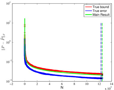
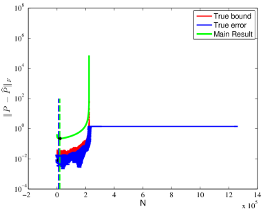
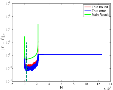
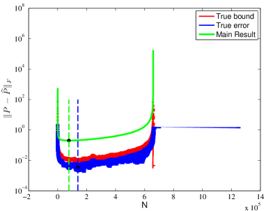
Figure 2: Norm of the perturbation using tangent plane radius $r$: (a) flat manifold with noise, (b) curved (tube-like) manifold with no noise, (c) curved (tube-like) manifold with noise, (d) curved manifold with noise. Dashed vertical lines indicate minima of the curves. Note the logarithmic scale on the Y-axes. See text for discussion.

The results are displayed in Figure 2. Panel (a) shows the noisy $(\sigma=0.01)$ curvature-free (linear subspace) result. As the only perturbation is due to noise, we expect the error to decay as $1/\sqrt{N}$ as the scale increases. The curves are shown on a logarithmic scale (for the Y-axis) and decrease monotonically, indicating the expected decay. Our bound (green) accurately tracks the behavior of the true error (blue) and is nearly identical to the true bound (red). Panel (b) shows the results for a noise-free manifold with principal curvatures given in Table 1 such that $K=12.6025$. Notice that three of the normal directions exhibit high curvature while the others are flatter, giving a tube-like structure to the manifold. In this case, perturbation is due to curvature only and the error increases monotonically (ignoring the slight numerical instability at extremely small scales), as predicted in the discussion of Sections 1.2 and 3.1. Eventually, a scale is reached at which there is too much curvature and the bounds blow up to infinity. This corresponds exactly to where the true error plateaus at its maximum value, indicating that the computed subspace is now orthogonal to the true tangent space. In this case, condition 1 of Theorem 3.2 is violated as there is no longer separation between the linear and curvature spectra, $\delta^{-1}$ becomes large, and our analysis predicts that the computed eigenspace contains a direction orthogonal to the true tangent space.

Figure 2c shows the results for a noisy ($\sigma=0.01$) version of the manifold used in panel (b). Note that the error is large at small scales due to noise and large at large scales due to curvature. At these scales the bounds are accordingly ill conditioned and track the behavior of the true error when well conditioned. Figure 2d shows the results for a manifold again with $K=12.6025$, but with the principal curvatures equal in all normal directions ($\kappa_{i}^{(j)}=1.0189$ for $i=1,\dots,3$ and $j=4,\dots,20$), and noise ($\sigma=0.01$) is added. We observe the same general behavior as seen in panel (c), but both the true error and the bounds remain well conditioned at larger scales. This is explained by the fact that higher curvature is encountered at smaller scales for the manifold corresponding to panel (c) but is not encountered until larger scales in panel (d). Similar results are shown in Figure 3 for a 2-dimensional, noise-free saddle ($\kappa_{1}^{(3)}=3,\kappa_{2}^{(3)}=-3$) embedded in $\operatorname{\mathbb{R}}^{3}$, demonstrating an accurate bound for the case of principle curvatures of mixed signs.

The true bound (red) tightly tracks the true error (blue) and is tighter than our bound (green) in all cases except for the curvature-free setting, where a difference on the order of $10^{-3}$ is observed. This curvature-free bound may be understood by observing that the noise analysis is more precise than that for the curvature (see appendices) and that the height of the bound is controlled by the probability-dependent constants, which have been fixed across all plots for consistency. In fact, it is possible to choose the probability-dependent constants much larger for the curvature-free setting without violating Condition 2. Doing so increases the height of the bound (green) to match the height of the “true bound” (red) curve (result not shown). Note that a similar increase for nonzero curvature results in a curve that violates Condition 2.

In all of the presented experiments, the bound accurately tracks the behavior of the true error. In fact, the curves are shown to be parallel on a logarithmic scale, indicating that they differ only by multiplicative constants. These observations further indicate that the triangle inequalities used in bounding the norms $\|U_{m}^{T}\Delta U_{n}\|_{F}$, $m,n=\{1,2\},$ are reasonably tight. As no matrix decompositions are needed to compute our bounds, we have efficiently tracked the tangent space recovery error. The dashed vertical lines in Figure 2 indicate the locations of the minima of the true error curve (dashed blue) and the Main Result bound (dashed green). In general, we see agreement of the locations at which the minima occur, indicating the scale that will yield the optimal tangent space approximation. The minimum of the Main Result bound falls within a range of scales at which the true recovery error is stable. In particular, we note that when the location of the bound’s minimum does not correspond with the minimum of the true error (such as in panel (d)), the discrepancy occurs at a range of scales for which the true error is quite flat. In fact, in panel (d), the difference between the error at the computed optimal scale and the error at the true optimal scale is on the order of $10^{-2}$. Thus the angle between the computed and true tangent spaces will be less than half of a degree and the computed tangent space is stable in this range of scales. For a large data set it is impractical to examine every scale and one would instead most likely use a coarse sampling of scales. The true optimal scale would almost surely be missed by such a coarse sampling scheme. Our analysis indicates that despite missing the exact true optimum, we may recover a scale that yields an approximation to within a fraction of a degree of the optimum.

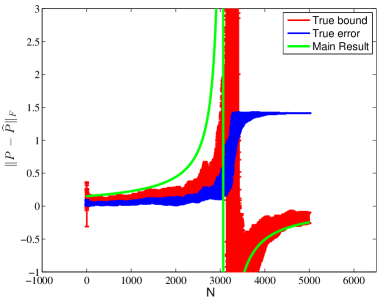
Figure 3: Bounds for a 2-dimensional saddle (noise free) with $\kappa_{1}^{(3)}=3$ and $\kappa_{2}^{(3)}=-3$.

4.2 Sensitivity to Error in Parameters

As is often the case in practice, parameters such as intrinsic dimension, curvature, and noise level are unknown and must be estimated from the data. It is therefore important to experimentally test the sensitivity of tangent space recovery to errors in parameter estimation. In the following experiments, we test the sensitivity to each parameter by tracking the optimal scale as one parameter is varied with the others held fixed at their true values. For consistency across experiments, the optimal scale is reported in terms of neighborhood radius and denoted by $r^{*}$. The relationship between neighborhood radius $r$ and number of sample points $N$ is defined by equation (7). In all experiments, we generate data sets sampled from a 4-dimensional manifold embedded in $\operatorname{\mathbb{R}}^{10}$ according to the local model (6).

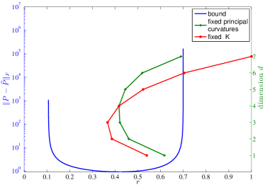
(a) $\kappa_{j}^{(i)}=2$, $\sigma=0.01$

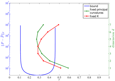
(b) $\kappa_{j}^{(i)}=3$, $\sigma=0.01$

Figure 4: The optimal radius is shown to be sensitive to error in estimates of $d$. The Main Result bound (blue) tracks the subspace recovery error (left ordinate). The green and red curves show the computed optimal radii for varying $d$ (right ordinate) with fixed $\kappa_{j}^{(i)}$ and fixed $K$, respectively. See text for details.

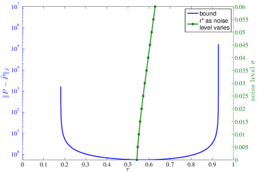
(a) $\kappa_{j}^{(i)}=1.5$, $\sigma=0.025$

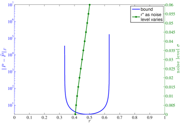
(b) $\kappa_{j}^{(i)}=2$, $\sigma=0.05$

Figure 5: The sensitivity to error in estimates of $\sigma$ is shown to be mild. The Main Result bound (blue) tracks the subspace recovery error (left ordinate) and the optimal radius is computed (green) for varying values of $\sigma$ (right ordinate). See text for details.

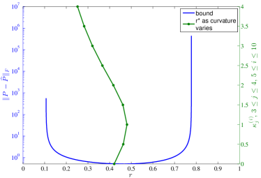
(a) $K=12.25$, $\sigma=0.01$

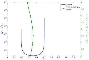
(b) $K=19.6$, $\sigma=0.025$

Figure 6: The sensitivity to error in estimates of curvature is shown to be mild. The Main Result bound (blue) tracks the subspace recovery error and the optimal radius is computed (green) for varying values of $\kappa_{3}^{(i)}$ and $\kappa_{4}^{(i)}$ with $\kappa_{1}^{(i)}$ and $\kappa_{2}^{(i)}$ held fixed. See text for details.

Figure 6 shows that the optimal scale $r^{*}$ is sensitive to errors in the intrinsic dimension $d$. A data set is sampled from a noisy, bowl-shaped manifold with equal principal curvatures in all directions. We set the noise level $\sigma=0.01$ and the principal curvatures $\kappa_{j}^{(i)}=2$ in panel (a) and $\kappa_{j}^{(i)}=3$ in panel (b). Noting that the true intrinsic dimension is $d=4$, we test the sensitivity of $r^{*}$ as $d$ is varied. There are three axes in each panel of Figure 6: the neighborhood radius $r$ on the abscissa; the angle $\|P-\widehat{P}\|_{F}$ on the left ordinate; and the values used for the dimension $d$ on the right ordinate. Our Main Result bound is shown in blue and tracks the subspace recovery error (angle, on the left ordinate) as a function of neighborhood radius $r$ for the true values of $d$, $\sigma$ and $\kappa_{j}^{(i)}$. Holding the noise and curvature fixed, we then compute $r^{*}$ using incorrect values for $d$ ranging from $d=1$ to $d=7$. The green and red curves show the computed $r^{*}$ for each value of $d$ (on the right ordinate) according to the two ways to fix curvature while varying $d$: (1) hold the value of each $\kappa_{j}^{(i)}$ fixed, thereby allowing $K$ to change with $d$ (shown in green); or (2) hold $K$ fixed, necessitating that the $\kappa_{j}^{(i)}$ change with $d$ (shown in red). The Main Result bound (blue) indicates an optimal radius of $r^{*}\approx 0.45$ in (a) and $r^{*}\approx 0.30$ in (b). However, the $r^{*}$ computed using inaccurate estimates of $d$ show great variation, ranging between a radius close to the optimum and a radius close to the size of the entire manifold. These experimental results indicate the importance of properly estimating the intrinsic dimension of the data.

Next, the sensitivity to error in the estimated noise level is shown to be mild in Figure 6. A data set is sampled from a noisy, bowl-shaped manifold with equal principal curvatures in all directions. The true values for the parameters are: $d=4$, $\kappa_{j}^{(i)}=1.5$, and $\sigma=0.025$ in 6a; and $d=4$, $\kappa_{j}^{(i)}=2$, and $\sigma=0.05$ in 6b. Our Main Result bound (blue) tracks the subspace recovery error (left ordinate) as a function of $r$ (abscissa) using the true parameter values and indicates an optimal radius of $r^{*}\approx 0.55$ and $r^{*}\approx 0.5$ for (a) and (b), respectively. Holding the dimension and curvature constant, we then compute $r^{*}$ using incorrect values for $\sigma$ ranging from $\sigma=0$ to $\sigma=0.06$. The green curve shows the computed $r^{*}$ for each value of $\sigma$ (on the right ordinate). In both 6a and 6b, the computed $r^{*}$ remain close to the optimum as the noise level varies and are within the range of radii where the recovery is stable (as indicated by the Main Result bound in blue). This behavior is in agreement with our experimental observations (not shown) indicating that increasing the noise level reduces the range for stable recovery but leaves the minimum of the Main Result bound relatively unaltered. We note that the range for stable recovery is smaller in (b) as is expected in the higher curvature and noise setting.

Finally, Figure 6 shows mild sensitivity to error in estimated curvature. A data set is sampled from a noisy manifold with two large principal curvatures ($\kappa_{1}^{(i)}$ and $\kappa_{2}^{(i)}$) and two small principal curvatures ($\kappa_{3}^{(i)}$ and $\kappa_{4}^{(i)}$) in each normal direction $i$. This tube-like geometry provides more insight for sensitivity to error in curvature by avoiding the more stable case where all principal curvatures are equal. The true values for the parameters are: $d=4$, $\sigma=0.01$, $\kappa_{1}^{(i)}=\kappa_{2}^{(i)}=2$, and $\kappa_{3}^{(i)}=\kappa_{4}^{(i)}=0.5$ for $5\leq i\leq 10$ in (a); and $d=4$, $\sigma=0.025$, $\kappa_{1}^{(i)}=\kappa_{2}^{(i)}=3$, and $\kappa_{3}^{(i)}=\kappa_{4}^{(i)}=1$ for $5\leq i\leq 10$ in (b). Our Main Result bound (blue) tracks the subspace recovery error (left ordinate) as a function of $r$ (abscissa) using the true parameter values and indicates an optimal radius of $r^{*}\approx 0.45$ and $r^{*}\approx 0.35$ for (a) and (b), respectively. Holding the dimension, noise level, and large principal curvatures $\kappa_{1}^{(i)}$ and $\kappa_{2}^{(i)}$ constant, we then compute the $r^{*}$ using incorrect values for the smaller principal curvatures $\kappa_{3}^{(i)}$ and $\kappa_{4}^{(i)}$, $5\leq i\leq 10$. The green curve shows the $r^{*}$ computed for values of $\kappa_{3}^{(i)}=\kappa_{4}^{(i)}$ indicated on the right ordinate, $5\leq i\leq 10$. The computed $r^{*}$ remain within the range of radii where the recovery is stable (as indicated by the Main Result bound in blue) in both (a) and (b). We observe less variation in the higher curvature and higher noise case shown in 6b. In this case, the larger principal curvatures anchor the bound, leaving $r^{*}$ less sensitive to error in the estimated smaller principal curvatures. As can be expected, experimental results (not shown) indicate that $r^{*}$ is sensitive to perturbations of these anchoring, large principal curvatures.

5 Practical Application & Experimental Results II

With the purpose of providing perturbation bounds that can be used in practice, we provide in this section the algorithmic tools that make it possible to directly apply the theoretical results of Section 3 to a real dataset.

The first tool is a “translation rule” to compare distances measured in the tangent plane ${T_{x_{0}}\negthinspace\mathcal{M}}$ and distances in $\operatorname{\mathbb{R}}^{D}$: given a point $x$ at a distance $R$ from the origin, we provide an estimate, $\hat{r}(R)$, of the distance of the projection of $x$ in ${T_{x_{0}}\negthinspace\mathcal{M}}$ to the origin $x_{0}$. The second tool is a plug-in method to compute a “clean estimate”, $\hat{x}_{0}$, of the point $x_{0}$ on $\mathcal{M}$ that serves as the origin of the coordinate system in our analysis. Equipped with these two tools, the practitioner can compute the perturbation bound as a function of the radius $R$ measured from $\hat{x}_{0}$ in the ambient space $\operatorname{\mathbb{R}}^{D}$.

5.1 Effective Distance in the Tangent Plane ${T_{x_{0}}\negthinspace\mathcal{M}}$

Our Main Result, Theorem 3.2, is presented in terms of the radius $r$ corresponding to the distance from the origin $x_{0}$ of a point’s noise-free tangential component. Because $r$ cannot be observed in practice, we provide an estimate $\hat{r}(R)$ of $r$ for any point $x$ at distance $R$ from the origin. In the presentation that follows, we assume oracle knowledge of the local origin $x_{0}\in\mathcal{M}$; recovery of this origin is addressed in the next section.

As previously introduced, a point $x$ in a neighborhood of $x_{0}$ may be decomposed as $x=x_{0}+\ell+c+e$ and we recognize $r^{2}=\|\ell\|^{2}$. To explore the relationship between $r$ and $R$, we compute

$$R^{2}=\|x-x_{0}\|^{2}=\|x_{0}+\ell+c+e-x_{0}\|^{2}=r^{2}+\|c\|^{2}+\|e\|^{2}+2\langle\ell+c,e\rangle,$$ (34)

where we use that $\langle\ell,c\rangle=0$. The terms on the right hand side depend on the realizations of the sample point $x$ and noise $e$. To understand their sizes, we compute in expectation,

$$\mathbb{E}[\|c\|^{2}]=\gamma r^{4},\quad\mathbb{E}[\|e\|^{2}]=\sigma^{2}D,\quad\text{and}\quad\mathbb{E}[\langle\ell+c,e\rangle]=0,$$

where

$$\gamma=\frac{\sum_{i=d+1}^{D}3K_{nn}^{ii}+K_{mn}^{ii}}{2(d+2)(d+4)}.$$ (35)

Injecting these terms into (34), we solve for positive and real $r$ and arrive at an approximation $\hat{r}(R)$ of the (tangent plane) radius $r$ given the observable (ambient) radius $R$:

$$\hat{r}(R)=\sqrt{\frac{1}{2\gamma}\left(-1+\sqrt{1+4\gamma(R^{2}-\sigma^{2}D)}\right)}.$$ (36)

Remark 5.1.

Another approach to determine the relationship between $r$ and $R$ proceeds as follows. We calculate the volume of the $d$-dimensional ball $B^{d}_{x_{0}}(r)$ given by the pre-image of the points in the ball $B^{D}_{x_{0}}(R)$ of radius $R$ in $\operatorname{\mathbb{R}}^{D}$, and use this volume to derive an effective radius $r$.

In the noise-free case, we can get some insight into this problem using a result from Gray Gray74 that gives the volume of a geodesic ball $B^{\mathcal{M}}_{x_{0}}(\omega)$ on $\mathcal{M}$ centered at $x_{0}$ as a function of the radius $\omega$ measured along the manifold. We have

$$V(B^{\mathcal{M}}_{x_{0}}(\omega))=\omega^{d}v_{d}\left(1-\frac{S(x_{0})}{6(n+2)}\omega^{2}+o(\omega^{2})\right),$$

where $S(x_{0})$ is the scalar curvature of the manifold at $x_{0}$ and $v_{d}$ is the volume of the $d$-dimensional unit ball. Let $r$ be the radius of the smallest ball that encloses the pre-image of $B^{\mathcal{M}}_{x_{0}}(\omega)$ in the tangent plane ${T_{x_{0}}\negthinspace\mathcal{M}}$,

$$\forall\ell=(\ell_{1},\ldots,\ell_{d})\in B^{d}_{x_{0}}(r),\quad x=\begin{bmatrix}\ell_{1}&\cdots&\ell_{d}&f_{d+1}(\ell)&f_{D}(\ell)\end{bmatrix}\in B^{\mathcal{M}}_{x_{0}}(\omega).$$

In our coordinate system, $B^{d}_{x_{0}}(r)$ is the smallest ball that encloses the projection of $B^{\mathcal{M}}_{x_{0}}(\omega)$ in the tangent plane ${T_{x_{0}}\negthinspace\mathcal{M}}$, and therefore the volume of $B^{d}_{x_{0}}(r)$ is smaller than the volume of $B^{\mathcal{M}}_{x_{0}}(\omega)$. Finally, we note that $V(B^{\mathcal{M}}_{x_{0}}(\omega))$ corresponds to the volume of an “effective ball” in $\operatorname{\mathbb{R}}^{d}$ of radius $r_{eff}$,

$$r_{eff}=\omega\left(1-\frac{S(x_{0})}{6(d+2)}\omega^{2}+o(\omega^{2})\right)^{1/d}.$$ (37)

Because $V(B^{d}_{x_{0}}(r))\leq V(B^{\mathcal{M}}_{x_{0}}(\omega))=V(B^{d}_{x_{0}}(r_{eff}))$, we have $r\leq r_{eff}$. We note that if $\omega$ is small, we can approximate the chordal distance $R$ with the geodesic distance $\omega$. If we use $r_{eff}$ as an estimate for $r$, we obtain

$$r\approx R\left(1-\frac{S(x_{0})}{6(d+2)}R^{2}\right)^{1/d}\approx R\left(1-\frac{S(x_{0})}{6d(d+2)}R^{2}\right).$$ (38)

The computation of the sectional curvature in our coordinate system yields the following expression,

$$S(x_{0})=\sum_{\begin{subarray}{c}m,n=1\\ m\neq n\end{subarray}}^{d}~{}\sum_{i=d+1}^{D}\kappa^{(i)}_{m}\kappa^{(i)}_{n}=\sum_{i=d+1}^{D}K^{ii}_{mn},$$ (39)

using the notation defined in (24). We finally obtain the following estimate of $r$,

$$R\left(1-\frac{\sum_{i=d+1}^{D}K^{ii}_{mn}}{6d(d+2)}R^{2}\right).$$ (40)

In comparison, the estimate $\hat{r}(R)$ given by (36) is approximately equal to

$$R\left(1-\frac{\sum_{i=d+1}^{D}3K_{nn}^{ii}+K_{mn}^{ii}}{4(d+2)(d+4)}R^{2}\right),$$ (41)

for small values of $R$. The two estimates, which capture the effect of curvature on the relationship between $r$ and $R$, are indeed very similar, confirming the general form of the approximation given by (36).

Remark 5.2.

In a manner similar to the previous derivation, we can estimate the effect of the noise on the volume a ball $B^{D}_{x_{0}}(R)$ of noisy samples centered around $x_{0}$. We define the normal space ${N_{x_{0}}\negthinspace\mathcal{M}}$ to be the orthogonal complement of ${T_{x_{0}}\negthinspace\mathcal{M}}$ in $\operatorname{\mathbb{R}}^{D}$. When $D$ is sufficiently large, we expect that the Gaussian noise will concentrate on the surface of a sphere of radius $\sigma\sqrt{D}$. The probability density function of the noisy samples is given by the convolution of the uniform distribution on the manifold (seen as a distribution in $\operatorname{\mathbb{R}}^{D}$ localized on $\mathcal{M}$) with the Gaussian kernel. If the manifold is flat, the probability density function of the noisy samples points $X$ becomes uniform in the tube

$$\mathcal{M}_{\sigma}=\left\{x=y+u,y\in\mathcal{M},u\in{N_{x_{0}}\negthinspace\mathcal{M}},\|u\|\leq\sigma\sqrt{D}\right\}.$$ (42)

Because the noisy points are spread uniformly in $\mathcal{M}_{\sigma}$, the measure of the set of noisy points in the ball centered at $x_{0}$ of radius $R$, $B^{D}_{x_{0}}(R)$, is given by

$$\frac{V_{D}(B^{D}_{x_{0}}(R)\cap\mathcal{M}_{\sigma})}{(2\sigma\sqrt{D})^{D-d}},$$ (43)

where the factor $1/(2\sigma\sqrt{D})^{D-d}$ accounts for the uniform distribution of the noisy points in $\mathcal{M}_{\sigma}$ along the direction ${N_{x_{0}}\negthinspace\mathcal{M}}$. We can approximate the set $B^{D}_{x_{0}}(R)\cap\mathcal{M}_{\sigma}$ by a smaller enclosed cylinder

$$B^{d}_{x_{0}}(\sqrt{R^{2}-d\sigma^{2}D})\oplus[-\sigma\sqrt{D},\sigma\sqrt{D}]^{D-d}$$

as soon as the radius $R$ extends beyond the tube $\mathcal{M}_{\sigma}$ in the direction ${N_{x_{0}}\negthinspace\mathcal{M}}$. This yields the following estimate for the volume of $V_{D}(B^{D}_{x_{0}}(R)\cap\mathcal{M}_{\sigma})$,

$$v_{d}(R^{2}-d\sigma^{2}D)^{d/2}(2\sigma\sqrt{D})^{D-d}.$$ (44)

We conclude that the set of noisy point in $B^{D}_{x_{0}}(R)$ has a measure given by

$$v_{d}(R^{2}-d\sigma^{2}D)^{d/2}=v_{d}\left[R\sqrt{1-\frac{d\sigma^{2}D}{R^{2}}}\;\right]^{d}$$ (45)

This measure corresponds to an effective radius $r$ in the tangent plane given by

$$r=R\sqrt{1-\frac{d\sigma^{2}D}{R^{2}}}.$$ (46)

Because we compute a lower bound on the measure of the set of noisy points in $B^{D}_{x_{0}}(R)$, the effective radius (46) introduces a correction $d\sigma^{2}D$ to $R^{2}$ that is $d$ times larger than the correction obtained in (36), $\sigma^{2}D$. While a more precise computation of $V_{D}(B^{D}_{x_{0}}(R)\cap\mathcal{M}_{\sigma})$ can remove the dependency on the dimension $d$, this computation confirms that the effect of noise can be accounted for by a simple subtraction of a term of the form $\sigma^{2}D$ from $R^{2}$, as indicated in the less formal calculation that leads to (36).

The same line of argument can be followed when the manifold is not flat. The authors in Genovese12 prove that when the noise is uniformly distributed along the normal fibers, then the probability distribution of the noisy points is still approximately uniform. The authors in Genovese12 bound the departure from the uniform distribution using geometric constants analogous to $\gamma$ or the scalar curvature $S$. Because the Gaussian will lead to a uniform distribution in the tube $\mathcal{M}_{\sigma}$, quantitatively similar result can be obtained when the noise a Gaussian, as confirmed by the thorough analysis performed in Maggioni-MIT ; LittleThesisDuke . While a more accurate estimate of $r$, which would account for curvature and noise, could be obtained using this route, our experiments in the next section indicate that the rough approximation provided by (36) accurately tracks the true $r$.

Let us examine the quality of the approximation of $r$ given by $\hat{r}(R)$ in (36) using the two data sets from Section 4 that correspond to Figures 2(c) and 2(d). The first data set consists of noisy ($\sigma=0.01$) points sampled from a 3-dimensional manifold embedded in $\mathbb{R}^{20}$, where the principal curvatures of the manifold are equal in all normal directions (“bowl geometry”). The second data set consists of noisy ($\sigma=0.01$) points sampled from a 3-dimensional manifold embedded in $\mathbb{R}^{20}$ where the principal curvatures (given in Table 1) are such that three of the normal directions exhibit significantly greater curvature than the others (“tube geometry”). Figure 7 shows the radius $r$ measured in the tangent plane (blue) and its estimate $\hat{r}(R)$ (black) given by (36). The radius $R$ measured in the ambient space, from which the estimate $\hat{r}(R)$ is computed, is shown in green for reference. The bowl geometry is shown in Figure 7(a) and the tube geometry is shown in Figure 7(b). We see that for both geometries, $r$ and $\hat{r}(R)$ are nearly indistinguishable over all relevant scales (the disagreement at the largest scales for the tube geometry occurs well after the computed tangent plane becomes orthogonal to the true tangent plane). The results shown in this figure indicate that $\hat{r}(R)$ can be used to reliably estimate $r$ from the observed $R$ and, therefore, to compute the Main Result bound (29) from quantities that are observable in practice.

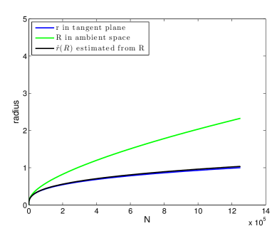
(a) bowl geometry

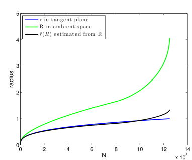
(b) tube geometry

Figure 7: The tangent plane radius $r$ (blue) and its approximation $\hat{r}(R)$ (black) given by equation (36) are shown to be indistinguishable over all relevant scales for two different geometries. The ambient radius $R$ from which the estimate $\hat{r}(R)$ is computed is shown in green. See text for discussion.

5.2 Subspace Tracking and Recovery using the Ambient Radius

We now repeat the experiments of Section 4.1 by recomputing the subspace recovery error and subspace recovery bounds using the radius in the ambient space, $R$, in place of the tangent plane radius, $r$. We demonstrate that, after converting the ambient radius $R$ to its corresponding tangent plane radius $\hat{r}(R)$, the bound presented in the Main Result Theorem 3.2 accurately tracks the subspace recovery error. The presented results demonstrate that the Main Result may be used for tangent space recovery in the practical setting where only the ambient radius is available.

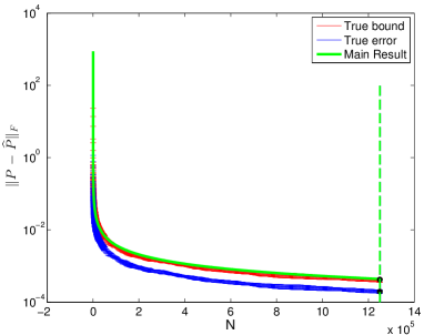
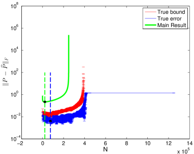
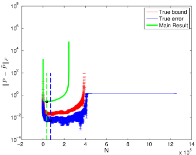
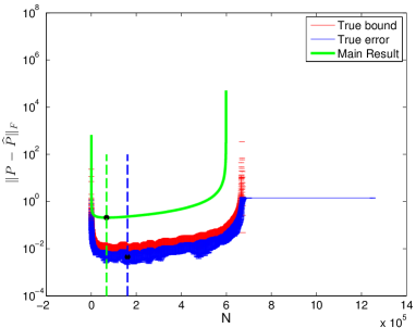
Figure 8: Norm of the perturbation using the ambient radius $R$: (a) flat manifold with noise, (b) curved (tube-like) manifold with no noise, (c) curved (tube-like) manifold with noise, (d) curved (bowl-like) manifold with noise. Dashed vertical lines indicate minima of the curves. Note the logarithmic scale on the Y-axes. Compare with Figure 2 and see text for discussion.

We begin by generating 3-dimensional data sets embedded in $\mathbb{R}^{20}$ according to the specifications given in Section 4.1. The curvature is chosen such that $K=12.6025$ for all manifolds (excluding the linear subspace example). The tube geometry is implemented by choosing principal curvatures as given in Table 1 and the bowl geometry has all principal curvatures set to 1.0189. All but the noise-free data set have Gaussian noise added with standard deviation $\sigma=0.01$.

For each experiment, the ambient radius $R$ is measured from the data and used to approximate the corresponding tangent plane radius $\hat{r}(R)$ by equation (36), from which we compute our bound (29). We then compare this bound with the true subspace recovery error. Mimicking the experiments of Section 4.1, the tangent plane at the local origin $x_{0}$ is computed at each scale $N$ via PCA of the $N$ nearest neighbors of $x_{0}$, where the distance from $x_{0}$ (the radius $R$) is now measured in the ambient space $\mathbb{R}^{D}$. The true subspace recovery error $\|P-\widehat{P}\|_{F}$ is then computed at each scale. The “true bound” is again computed by applying Theorem 2.4 after measuring each perturbation norm directly from the data. We recall that this “true bound” requires no SVDs and utilizes information that is not practically available to represent the best possible bound that we can hope to achieve. We will compare the mean of the true error and mean of the true bound over 10 trials (with error bars indicating one standard deviation) to the bound given by our Main Result in Theorem 3.2, holding with probability greater than 0.8. We note that for these experiments, the local origin $x_{0}$ is given by oracle information and we will consider its recovery in a separate set of experiments.

The results are shown in Figure 8 and should be compared with those shown in Figure 2. Panel (a) shows the noisy curvature-free (linear subspace) result and we observe that the behaviors of the true error (blue), true bound (red), and main result bound (green) match the behaviors of their counterparts in Figure 2(a) that were computed using $r$. In particular, the error in Figure 8(a) decays as $1/\sqrt{N}$ (note the logarithmic scale of the Y-axis). Our bound (green) accurately tracks the true error (blue) and is nearly indistinguishable from the true bound (red). Panel (b) shows the result for a noise-free manifold with tube geometry such that three of the normal directions exhibit high curvature while the others are flatter. We see that, much like in Figure 2(b), the main result bound (green) increases monotonically (ignoring the slight numerical instability at extremely small scales) to match the general behavior of the true error (blue) and true bound (red). Panel (c) shows the results for the noisy version of the manifold used in panel (b). We observe that our bound (green) now exhibits blow up at small scales due to noise and blow up at large scales due to curvature, matching the behavior of the true error. Finally, panel (d) shows the results for the noisy manifold with bowl geometry where all principal curvatures are equal, and indicates that our bound tracks the error at all scales. The dashed vertical lines in Figure 8 indicate the locations of the minima of the true error curves (dashed blue) and the Main Result bounds (dashed green). We see that the location of the minimum of the Main Result bound is, in general, close to the minimum of the true error curve and falls within a range of scales for which the error is quite flat.

We observe that the results using $R$ in Figure 8 are similar to those seen in Figure 2 using $r$, while noting that the true error for the tube geometry remains stable at larger scales in Figure 8 than the true error in Figure 2. To understand this observation, we examine the effect of geometry on the radii $R$ and $r$. Figure 9 shows the radius $R$ in green for the bowl geometry (left) and for the tube geometry (right). This radius corresponds to the norm of each point $x$ collected as a ball is grown in the ambient space. Shown in red is the ambient radius of each point $x$ collected as the tangent plane radius, $r$, is grown. This curve corresponds to the collection of points according to the norm of their tangential projection. Figure 9 shows that these radii exhibit different behaviors depending on the geometry of the manifold. When all principal curvatures are equal (bowl geometry), each normal direction exerts the same amount of influence on a point’s norm and curvature does not impact the order in which the points are discovered. Thus, the radii are shown to be identical for the bowl geometry in Figure 9(a), with the green curve sitting exactly on top of the red curve. However, the tube geometry allows for curvature in certain normal directions to exert more influence on the norm than others. In this situation, growing a ball in the ambient space will necessarily discover points exhibiting greater curvature at the larger scales. In contrast, the ball grown in the tangent space may discover such points at much smaller scales, as the radius measures the norm of only the tangential components. Thus, at a given scale $r$ of the ball in the tangent plane, we will have collected points exhibiting different amounts of curvature in the unbalanced tube geometry setting. This is seen in Figure 9(b), where the ambient radius of the collected points is much larger at a given scale when growing a ball in the tangent plane (red curve) than when growing a ball in the ambient space (green curve). These observations imply that the true tangent space recovery error is sensitive to the balance, or lack thereof, of the geometry. Finally, due to this sensitivity to the strongly anisotropic tube geometry, we notice that the true error indicates orthogonality at scales larger than indicated by our bound. The minimum of our bound therefore remains within the range of scales that provide stable recovery.

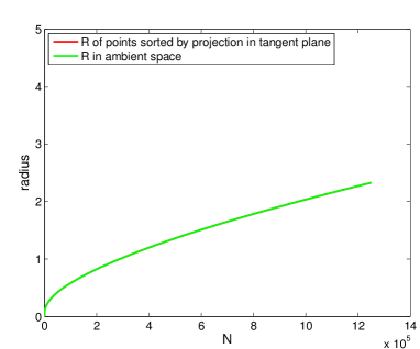
(a) bowl geometry

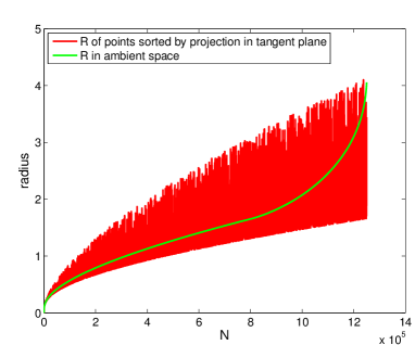
(b) tube geometry

Figure 9: The radius $R$ is shown sorted according to the order in which points are discovered in the ambient space (green) and according to the order in which points are discovered when projected in the tangent plane (red). The ordering is identical for the bowl geometry (left), where the green curve is on top of the red curve, because all principal curvatures are equal. The ordering is very different for the tube geometry (right) where some directions exhibit greater curvature than others. See text for discussion.

We conclude this experimental section by noting that equation (36) provides only an approximation to $r$ and we therefore expect that tighter results are possible. This avenue should be the subject of future investigation. Nonetheless, the experimental results presented in this section indicate that our Main Result Theorem 3.2 may be used, with suitable modification according to (36), to track the tangent space recovery error in the practical setting where only the ambient radius $R$ is available to the user.

Having demonstrated the utility of the Main Result Theorem 3.2, we now turn our attention to the recovery of the unknown local origin.

5.3 Finding the Local Origin

As explained previously, here we propose a “plug-in” to compute a “clean estimate”, $\hat{x}_{0}$, of the point $x_{0}$ on $\mathcal{M}$ that serves as the origin of the coordinate system in our analysis. At first glance, it might seem that a useful perturbation bound should assume that the analysis is centered around a noisy point and account for this additional source of uncertainty. We advocate that this is an unnecessarily pessimistic perspective, and we therefore offer an alternate approach: we show that a reliable estimate, $\hat{x}_{0}$, of $x_{0}$ can be computed from a noisy data set. Using $\hat{x}_{0}$, the reader can directly apply the theoretical bounds found in Section 3 to analyze a noisy set of points. The algorithm to compute $\hat{x}_{0}$ is simple and computationally inexpensive (requiring no matrix decompositions), and makes use of the geometric information encoded in the trajectory of the points’ center of mass over several scales. It is worth mentioning that we expect the proposed algorithm to be a universal first step for a local, multiscale analysis of the type presented in this paper. Further intuition, details, and experiments are presented below.

It is important to clearly state the role of $x_{0}$ in the practical implementation of this work: given a noisy point $y\in\mathbb{R}^{D}$ selected by the user, $x_{0}$ is the closest point on the “clean” manifold $\mathcal{M}$ around which we want to estimate the tangent plane ${T_{x_{0}}\negthinspace\mathcal{M}}$. Since we assume that $\mathcal{M}$ is smooth, there exists a neighborhood about $x_{0}$ where the manifold is described by the model (6), and $x_{0}$ is the origin of this model. Because $x_{0}$ is the projection of $y$ on $\mathcal{M}$, $y-x_{0}$ is normal to ${T_{x_{0}}\negthinspace\mathcal{M}}$, and the points $y$ and $x_{0}$ therefore have the same coordinates in the tangential directions. Rotating the coordinate system to align the axes with these directions, our goal is to move from $y$ to $x_{0}$ in the directions normal to the tangent plane. Figure 10 provides an illustration of this framework. We remark that the rotation of the coordinate axes is merely for notational convenience and will be discussed below.

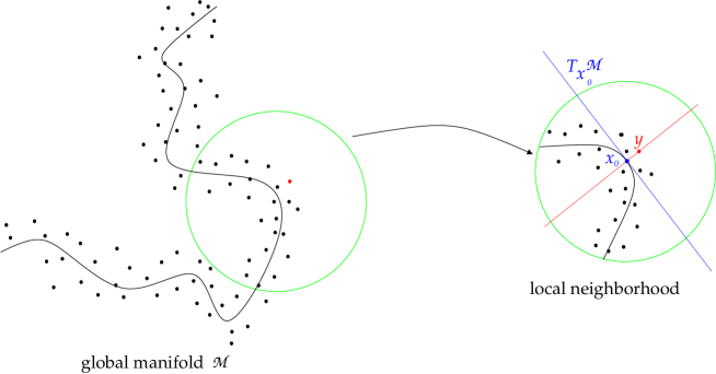
Figure 10: Left: the user selects a noisy point $y$ (in red) close to the smooth manifold $\mathcal{M}$. Right: a local neighborhood is extracted. The point $x_{0}$ (blue) that is closest to $y$ on the manifold becomes the point at which we compute ${T_{x_{0}}\negthinspace\mathcal{M}}$ (blue). The local coordinate system is defined by the tangent plane ${T_{x_{0}}\negthinspace\mathcal{M}}$ (blue) and the normal space ${N_{x_{0}}\negthinspace\mathcal{M}}$ (red). Neither the computation of the perturbation bound nor the estimation of $x_{0}$ require that the unknown rotation be estimated.

Our strategy will be to compute the center of mass $\overline{X}$ about $y$ and track the trajectory of each coordinate of $\overline{X}$ as the radius about $y$ grows from small to large scales. We use the term “trajectory” to refer to the coordinate(s) of the sequence of sample means $\overline{X}$ computed over growing radii. As we will see, these trajectories contain all of the geometric information necessary to recover $x_{0}$ and is robust to the presence of noise. The steps for recovering $x_{0}$ are given below as Algorithm 1.

Algorithm 1 Recovering the Local Origin $x_{0}$

Input: Noisy points $X=\{x^{(i)}\}_{i=1}^{N}$, reference point $y\in\mathbb{R}^{D}$, scale intervals $\{\mathcal{I}^{(m)}\}_{m=1}^{M}$ such that $\mathcal{I}^{(m)}=[R^{(m,1)},R^{(m,2)}]$ with $R^{(m,1)}<R^{(m,2)}~{}\forall m$ and $\begin{cases}R^{(p,1)}\leq R^{(q,1)}\\ R^{(p,2)}\leq R^{(q,2)}\end{cases}$ for $p>q$
Outpt: Estimate $\widehat{x}_{0}$ of the local origin $x_{0}\in\mathcal{M}$

FOR each scale interval $\mathcal{I}^{(m)},m=1,\dots,M$:

1. Center a ball at $y$ and compute $\overline{X}=\frac{1}{N_{B}}\sum_{i=1}^{N_{B}}x^{(i)}$, the mean of the points inside the ball $B^{D}_{y}(R_{y})$, $\forall R_{y}\in\mathcal{I}^{(m)}$, where $N_{B}=|B^{D}_{y}(R_{y})|$.

2. FOR each coordinate $j=1,\dots,D$:

   1. Fit (in the least squares sense) the trajectory of $\overline{X}_{j}$ to the model

      $$q_{y}(R_{y})=\beta_{2}R_{y}^{2}+\beta_{0},$$

      over the range of scales in $\mathcal{I}^{(m)}$, explicitly requiring a zero first derivative at $R_{y}=0$

   2. Set $\widehat{x}_{0_{j}}^{(m)}=\beta_{0}$

3. END

4. Set $y=\widehat{x}_{0}^{(m)}$

END

Return $\widehat{x}_{0}=\widehat{x}_{0}^{(M)}$ as the estimate of the local origin

The trajectory of each coordinate of $\overline{X}$ will be noisy and unreliable at very small scales. However, due to the averaging process, the uncertainty from both the noise and the random sampling is overcome at large scales. Thus, the large scale trajectory reaches a “steady state behavior” that is essentially free of uncertainty and encodes information about the initial state, i.e., the noise-free trajectory very close to $x_{0}$.

Remark 5.3.

The algorithm described in this section can be understood in the context of the estimation of the center location of the probability density associated with the clean point $x_{0}$ on $\mathcal{M}$. Indeed, our model assumes that a noisy point $x$ is obtained by perturbing a clean point $\ell+c$ by adding Gaussian noise. The probability distribution of the noisy points is thus given by the convolution of a $D$-dimensional Gaussian density $G_{\sigma}$ with the $D$-dimensional probability density $f_{\mathcal{M}}$ of the clean points, which is supported solely on $\mathcal{M}$,

$$f_{\mathcal{M}}\ast G_{\sigma}(x).$$

The goal of the algorithm is to recover the clean point $x_{0}$ around which $f_{\mathcal{M}}$ is localized, given some noisy realizations $X$ sampled from the probability density $f_{\mathcal{M}}\ast G_{\sigma}(x)$. This can be achieved by removing the effect of the blurring (a process known as deconvolution Genovese12b ) caused by $G_{\sigma}$, and computing a “sharp” estimate of the density $f_{\mathcal{M}}$ around $x_{0}$. There exists an expansive literature on such deblurring problems. A very successful approach consists in reversing the heat equation associated with the blurring at increasing scales (e.g., Perona90 ; Osher90 ). This idea is the essence of our algorithm. By tracking the centroid of a ball of decreasing size, we can extrapolate this trajectory in the limit where the ball has radius zero, and effectively compute $\lim_{\sigma\rightarrow 0}f_{\mathcal{M}}\ast G_{\sigma}(x_{0})$. This process yields the initial origin with very little uncertainty even for very high noise and high curvature.

Let us now provide further intuition for why such a procedure will work. The reader is asked to be mindful that we will only provide an overview of the results and that a rigorous development of the convergence properties is left for future work.

5.3.1 Center of Mass Trajectory

Following the local model (6) with origin $x_{0}$, a neighboring point $x$ has coordinates of the form

$$x=x_{0}+\ell+c+e=\begin{bmatrix}x_{0_{1}}\\ \\ \\ \vdots\\ \\ \\ x_{0_{D}}\end{bmatrix}+\begin{bmatrix}\ell_{1}\\ \vdots\\ \ell_{d}\\ \\ 0\\ \vdots\\ 0\end{bmatrix}+\begin{bmatrix}0\\ \vdots\\ 0\\ \\ c_{d+1}\\ \vdots\\ c_{D}\end{bmatrix}+\begin{bmatrix}e_{1}\\ \\ \\ \vdots\\ \\ \\ e_{D}\end{bmatrix},$$ (47)

and coordinate $j$ of $\overline{X}$ is of the form

$$\overline{X}_{j}=\frac{1}{N}\sum_{i=1}^{N}x^{(i)}_{j}=\begin{cases}x_{0_{j}}+\frac{1}{N}\sum_{i=1}^{N}\ell^{(i)}_{j}+\frac{1}{N}\sum_{i=1}^{N}e^{(i)}_{j},&j\leq d\\ x_{0_{j}}+\frac{1}{N}\sum_{i=1}^{N}c^{(i)}_{j}+\frac{1}{N}\sum_{i=1}^{N}e^{(i)}_{j},&j>d.\end{cases}$$ (48)

The sample mean $\overline{X}_{j}=\frac{1}{N}\sum_{i=1}^{N}x^{(i)}_{j}$ approximates $\mathbb{E}[x_{j}]$ with the uncertainty decaying as $1/\sqrt{N}$. More precisely, by the Hoeffding inequality and the Gaussian tail bound, we have the following intervals for coordinate $j$ at scale $N$:

$$\overline{X}_{j}\in\begin{cases}\Big{[}x_{0_{j}}-\frac{\sqrt{2}\xi}{\sqrt{N}}(r+\sigma),\;x_{0_{j}}+\frac{\sqrt{2}\xi}{\sqrt{N}}(r+\sigma)\Big{]},&j\leq d\\[8.0pt] \Big{[}\left(x_{0_{j}}+\frac{K_{j}r^{2}}{2(d+2)}\right)-\frac{\sqrt{2}\xi}{\sqrt{N}}\left(\frac{\sqrt{d}K_{j}^{(+)}r^{2}}{2}+\sigma\right),\;\left(x_{0_{j}}+\frac{K_{j}r^{2}}{2(d+2)}\right)+\frac{\sqrt{2}\xi}{\sqrt{N}}\left(\frac{\sqrt{d}K_{j}^{(+)}r^{2}}{2}+\sigma\right)\Big{]},&j>d\end{cases}$$ (49)

with probability greater than $1-6e^{-\xi^{2}}$. We see that while the coordinates exhibit variation about their means at small scales, they reach their average (steady state) behavior with high probability at large scales. Thus, the large scale coordinate trajectories are controlled with little uncertainty for densely sampled data.

Remark 5.4.

More generally, we expect to observe data in a rotated coordinate system. Consider the setting in $\mathbb{R}^{2}$ for a 1-dimensional manifold after applying a rotation to our conventional coordinate system. The observed coordinates will be of the form

$$\begin{pmatrix}\overline{X}_{1}\\ \overline{X}_{2}\end{pmatrix} =\begin{pmatrix}x_{0_{1}}\\ x_{0_{2}}\end{pmatrix}+\begin{pmatrix}Q_{11}&Q_{12}\\ Q_{21}&Q_{22}\end{pmatrix}\begin{pmatrix}\frac{1}{N}\sum_{i=1}^{N}\ell^{(i)}_{1}+\frac{1}{N}\sum_{i=1}^{N}e^{(i)}_{1}\\ \frac{1}{N}\sum_{i=1}^{N}c^{(i)}_{2}+\frac{1}{N}\sum_{i=1}^{N}e^{(i)}_{2}\end{pmatrix}$$

$$=\begin{pmatrix}x_{0_{1}}+Q_{11}\mathbb{E}[\ell]+Q_{12}\mathbb{E}[c]+(Q_{11}+Q_{12})\mathbb{E}[e]\pm\mathcal{O}\left(\frac{1}{\sqrt{N}}\right)\\ x_{0_{2}}+Q_{21}\mathbb{E}[\ell]+Q_{22}\mathbb{E}[c]+(Q_{21}+Q_{22})\mathbb{E}[e]\pm\mathcal{O}\left(\frac{1}{\sqrt{N}}\right)\end{pmatrix}\quad\text{(w.h.p.)}$$ (50)

$$=\begin{pmatrix}x_{0_{1}}+Q_{12}\frac{K_{2}r^{2}}{2(d+2)}\pm\mathcal{O}\left(\frac{1}{\sqrt{N}}\right)\\ x_{0_{2}}+Q_{22}\frac{K_{2}r^{2}}{2(d+2)}\pm\mathcal{O}\left(\frac{1}{\sqrt{N}}\right),\end{pmatrix}$$

where $Q=\left(\begin{smallmatrix}Q_{11}&Q_{12}\\ Q_{21}&Q_{22}\end{smallmatrix}\right)$ is a unitary matrix. We see that all coordinates have the same form as coordinates $j>d$ in (49) with the slight modification introduced by the $Q_{mn}$ terms. In general, we will observe a linear combination of all coordinates with weights $Q_{mn}<1$. In particular, all coordinates will be of leading order $r^{2}$ with a constant intercept (the origin), and all other orders of $r$ appear as finite sample uncertainty terms that decay as $1/\sqrt{N}$. Because an arbitrary rotation leaves all coordinates with the same form as that of the coordinates $j>d$ in equation (49), we proceed with the analysis of these coordinates without loss of generality.

Continuing from (49), we use a calculation similar to (34) to show that $r^{2}\approx R^{2}$ for small $r$. We therefore expect the coordinate trajectories ($j>d$) to be quadratic functions of the observed radius $R$ with intercept $x_{0}$ and zero first derivative at $R=0$. Fitting the observed trajectory of each coordinate to the model

$$q(R)=\beta_{2}R^{2}+\beta_{0}$$ (51)

provides the least squares estimate of the origin $\widehat{x}_{0_{j}}=\beta_{0}$. By explicitly enforcing the zero first derivative condition, the model (51) should be robust to uncertainty in the observed data at small scales. Moreover, initial estimates of $\widehat{x}_{0_{j}}$ may be obtained from the stable, large scale trajectories to anchor the small scale estimate using (51). We now examine this procedure in more detail.

5.3.2 Estimating $x_{0}$

Equation (49) confirms our intuition that the large scale trajectory, smoothed from the averaging process, is very stable due to the $1/\sqrt{N}$ decay of the finite sample uncertainty terms. We must now cast this trajectory in terms of an observable radius $R_{y}$, the radius of a ball in $\mathbb{R}^{D}$ centered about the point $y$ in the presence of noise. Recall that the intent of the following discussion is to informally derive the correct order for all terms, with complete rigor reserved for future work.

Consider first the effect of measuring the radius about a point other than $x_{0}$. Let $\tau$ denote the offset vector,

$$\tau=y-x_{0}=\Big{[}0~{}\cdots~{}0~{}~{}\tau_{d+1}\cdots~{}\tau_{D}\Big{]}^{T},$$

since $y$ and $x_{0}$ only differ in their normal components. A calculation similar to (34) shows

$$R_{y}^{2}=\|x-y\|^{2}=\|x_{0}+\ell+c-\tau-x_{0}\|^{2}=\|\ell\|^{2}+\|c-\tau\|^{2}\leq r^{2}+\gamma r^{4}+\|\tau\|^{2}.$$ (52)

Solving for $r^{2}$ and injecting into (49) yields the following expression for $\overline{X}_{j}$ (coordinates $j>d$) at scale $N$, holding with high probability:

$$\overline{X}_{j}\in\Bigg{[}a_{1}R_{y}+(x_{0_{j}}-a_{0})-\frac{\sqrt{2}\xi}{\sqrt{N}}a_{-1}\;,\;a_{1}R_{y}+(x_{0_{j}}-a_{0})+\frac{\sqrt{2}\xi}{\sqrt{N}}a_{-1}\Bigg{]},$$ (53)

$$\text{for}\;R_{y}>\sqrt{\|\tau\|^{2}+\frac{1}{4\gamma}},$$ (54)

where

$$a_{1}=\frac{K_{j}}{2(d+2)\sqrt{\gamma}},\quad a_{0}=\frac{K_{j}}{4(d+2)\gamma}+\mathcal{O}\left(\frac{1}{R_{y}}\right),$$ (55)

with uncertainty term

$$a_{-1}=\frac{1}{2}\sqrt{\frac{d}{\gamma}}K_{j}^{(+)}R_{y}-\frac{1}{4}\frac{\sqrt{d}}{\gamma}K_{j}^{(+)}+\mathcal{O}\left(\frac{1}{R_{y}}\right).$$ (56)

Next, reasoning in a manner similar to (34), we introduce the following correction for the presence of the noise, enlarging the radius $R_{y}$ in (53) by $\sigma\sqrt{D}$ :

$$R_{y}\leftarrow R_{y}+\sigma\sqrt{D}.$$

We finally rewrite (53) to yield the expression for $X_{j}$ (coordinates $j>d$) at scale $N$, holding with high probability:

$$\overline{X}_{j}\in\Bigg{[}a_{1}R_{y}+\left(x_{0_{j}}-a_{0}+a_{1}\sigma\sqrt{D}\right)-\frac{\sqrt{2}\xi}{\sqrt{N}}a_{-1}\;,\;a_{1}R_{y}+\left(x_{0_{j}}-a_{0}+a_{1}\sigma\sqrt{D}\right)+\frac{\sqrt{2}\xi}{\sqrt{N}}a_{-1}\Bigg{]},$$ (57)

$$\text{for}\;R_{y}>\sqrt{\|\tau\|^{2}+\frac{1}{4\gamma}},$$

with $a_{1}$ and $a_{0}$ as given by (55) and uncertainty term $a_{-1}$ now taking the form

$$a_{-1}=\frac{1}{2}\sqrt{\frac{d}{\gamma}}K_{j}^{(+)}R_{y}+\frac{1}{2}\sqrt{\frac{d}{\gamma}}K_{j}^{(+)}\sigma\sqrt{D}-\frac{1}{4}\frac{\sqrt{d}}{\gamma}K_{j}^{(+)}+\sigma+\mathcal{O}\left(\frac{1}{R_{y}}\right).$$ (58)

While (57) indicates that the large scale trajectory is linear in $R_{y}$, all of the necessary geometric information for Algorithm 1 to succeed is encoded in this trajectory. To see this, we proceed momentarily by taking a path slightly different from that of the proposed algorithm. Consider fitting the large scale trajectory to the model

$$q_{y}^{linear}(R_{y})=\alpha_{1}R_{y}+\alpha_{0}$$ (59)

over the range of scale $\mathcal{I}^{(m)}=[R_{y}^{(m,1)},R_{y}^{(m,2)}]$. Let $R_{y}^{(m,1)}$ correspond to $N^{(m,1)}$ points, $R_{y}^{(m,2)}$ correspond to $N^{(m,2)}$ points, $N^{(m,1)}<N^{(m,2)}$, and let $\widetilde{N^{(m)}}=(N^{(m,1)}+N^{(m,2)})/2$. The least squares fit of the large scale $\overline{X}_{j}$ trajectory to (59) yields the coefficients

$$\alpha_{1}\in\Bigg{[}a_{1}-\frac{\xi}{\sqrt{\widetilde{N^{(m)}}}}\sqrt{\frac{d}{2\gamma}}K_{j}^{(+)}\;,\;a_{1}+\frac{\xi}{\sqrt{\widetilde{N^{(m)}}}}\sqrt{\frac{d}{2\gamma}}K_{j}^{(+)}\Bigg{]}$$ (60)

$$\alpha_{0}\in\Bigg{[}\left(x_{0_{j}}-a_{0}+a_{1}\sigma\sqrt{D}\right)-\frac{\sqrt{2}\xi}{\sqrt{\widetilde{N^{(m)}}}}\left(\sigma+\frac{1}{2}\sqrt{\frac{d}{\gamma}}K_{j}^{(+)}\left(\sigma\sqrt{D}-\frac{1}{2\sqrt{\gamma}}\right)\right)\;,\\ \;\left(x_{0_{j}}-a_{0}+a_{1}\sigma\sqrt{D}\right)+\frac{\sqrt{2}\xi}{\sqrt{\widetilde{N^{(m)}}}}\left(\sigma+\frac{1}{2}\sqrt{\frac{d}{\gamma}}K_{j}^{(+)}\left(\sigma\sqrt{D}-\frac{1}{2\sqrt{\gamma}}\right)\right)\Bigg{]}.$$ (61)

Noting that the (rescaled) mean curvature $K_{j}$ is encoded in $a_{1}$ and $a_{0}$, we may recover a large scale estimate of $x_{0_{j}}$ by setting

$$\widehat{x}_{0_{j}}^{(m)}=\alpha_{0}-\alpha_{1}\sigma\sqrt{D}+\alpha_{1}^{2}\frac{(d+2)}{K_{j}}.$$ (62)

Then we have

$$\left|x_{0_{j}}-\widehat{x}_{0_{j}}^{(m)}\right|~{}\leq~{}\frac{\sqrt{2}\xi}{\sqrt{\widetilde{N^{(m)}}}}\left(\sigma+\frac{\sqrt{d}}{2\gamma}K_{j}^{(+)}\right)+\frac{\xi^{2}}{\widetilde{N^{(m)}}}\frac{d(d+2)}{2\gamma}\frac{(K_{j}^{(+)})^{2}}{|K_{j}|},$$ (63)

with high probability.

Remark 5.5.

The $k$th point of the $\overline{X}_{j}$ trajectory has an uncertainty term that decays as $1/\sqrt{k}$. For convenience, we have replaced the point-by-point uncertainty decay with a constant factor of $1/\sqrt{\widetilde{N^{(m)}}}$ above, where $\widetilde{N^{(m)}}$ is the number of points in the middle of the current interval. A more rigorous analysis would account for the heteroskedasticity of the sequence of sample means $\overline{X}_{j}$ and use, e.g., a weighted least squares fit to the model.

We may use these calculations to understand the initial large scale exploration performed by Algorithm 1. The estimate produced by the algorithm may be seen as the result of replacing the trajectory with a linear function of $R_{y}$ as given by (57). Then, discarding the data, we work only with this linear approximation over all $R_{y}$. By doing so, we are discarding the quadratic behavior expected at small scales near $x_{0}$, as this part of the trajectory is damaged by the noise. We then recover the expected quadratic behavior by fitting the linear approximation to the following quadratic model,

$$q_{y}^{quad}(R_{y})=\beta_{2}R_{y}^{2}+\beta_{0},$$ (64)

where the zero first derivative condition is explicitly enforced. The estimate for coordinate $j$ of $x_{0}$ has the form

$$\widehat{x}_{0_{j}}=\alpha_{0}+\alpha_{1}\mathscr{F}(\mathcal{I}^{(m)}),$$ (65)

where

$$\mathscr{F}(\mathcal{I}^{(m)})=\frac{(R_{y}^{(m,2)})^{2}+4R_{y}^{(m,2)}R_{y}^{(m,1)}+(R_{y}^{(m,1)})^{2}}{6(R_{y}^{(m,2)}+R_{y}^{(m,1)})}$$ (66)

is a function of the scale interval. Comparing to (62), this estimate is equivalent to the previous large scale procedure when we choose

$$\mathscr{F}(\mathcal{I}^{(m)})=\frac{\alpha_{1}(d+2)}{K_{j}}-\sigma\sqrt{D}.$$ (67)

This choice also can be shown to minimize the error of the estimate in (65). In summary, if we could very carefully select the range of scales to satisfy (67), which requires a priori knowledge of curvature, we could compute an estimate of $x_{0}$ in one step. While we cannot expect to choose exactly the right interval to satisfy (67), we observe in practice (see Section 5.3.3) that the decreasing sequence of intervals used by Algorithm 1 will contain a proxy that allows for an accurate estimate.

The result of this procedure is an estimate $\widehat{x}_{0}^{(m)}$ over scale interval $\mathcal{I}^{(m)}$ that is very close to the true $x_{0}$. Setting $y=\widehat{x}_{0}^{(m)}$, we are left with only a very small offset vector $\tau$:

$$\|\tau\|^{2}=\frac{2\xi^{2}}{\widetilde{N^{(m)}}}\left(\sigma^{2}D+\frac{\sigma\sqrt{d}}{\gamma}\sum_{j=1}^{D}K_{j}^{(+)}+\frac{d}{4\gamma^{2}}(K^{(+)})^{2}\right)+\mathcal{O}\left(\frac{1}{(\widetilde{N^{(m)}})^{3/2}}\right).$$ (68)

The trajectories $X_{j}$ may now be recomputed by centering a ball about $y=\widehat{x}_{0}^{(m)}$ and the fitting procedure is repeated over scale interval $\mathcal{I}^{(m+1)}$. The error bound (68) shows that if we keep the number of points sufficiently large (given a dense enough sampling), even at small scales, we can decrease the uncertainty on the estimate of $x_{0}$. The accurate estimation of $x_{0}$ by Algorithm 1 is demonstrated in the next section.

5.3.3 Experimental Results

In this section, we test the performance of Algorithm 1 on several data sets over a range of parameters and tabulate the results. MATLAB code implementing Algorithm 1 is available for download at http://www.danielkaslovsky.com/code.

Data sets of $N=50,000$ points sampled from $d$-dimensional manifolds embedded in $\mathbb{R}^{D}$ were generated according to the local model (6) in the same manner as for all other experiments (see Section 4.1). For each data set, the local origin $x_{0}\in\mathbb{R}^{D}$ was chosen by sampling each coordinate from $\mathcal{U}[-10,10]$, where $\mathcal{U}[a,b]$ is the uniform distribution supported on $[a,b]$. An initial reference point $y\in\mathbb{R}^{D}$ was chosen as specified in Table 2 and a random rotation was applied to both the data set and $y$. Seven different experiments were performed with parameters as listed in Table 2. For each experiment, Algorithm 1 was used to recover the local origin of 10 data sets starting from the randomly initialized reference point $y$. The $\ell^{\infty}$ error ($\max_{j}|x_{0_{j}}-\widehat{x}_{0_{j}}|$) and mean squared error ($\sum_{j=1}^{D}(x_{0_{j}}-\widehat{x}_{0_{j}})^{2}/D$) of each trial were recorded, with the mean and standard deviation over the 10 trials reported in Table 2. The scale intervals were fixed across all experiments to be: $\mathcal{I}^{(1)}=[0.5N,0.75N]$, $\mathcal{I}^{(2)}=[1,0.4N]$, $\mathcal{I}^{(3)}=[1,0.3N]$, and $\mathcal{I}^{(4)}=[1,0.25N]$.

Table 2: Parameters for the data sets used to test Algorithm 1 with the $\ell^{\infty}$ error and MSE reported over 10 trials (mean $\pm$ standard deviation).

			$\kappa_{n}^{(i)}$
			$(d+1)\leq i\leq D$		$\tau_{j}=y_{j}-x_{0_{j}}$
Experiment	$d$	$D$	$1\leq n\leq d$	$\sigma$	$(d+1)\leq j\leq D$	$\ell^{\infty}$ error	MSE
Baseline						0.01646	6.1321e-5
(bowl)	3	20	1.0189	0.05	$\mathcal{N}(0,4\sigma^{2})$	$\pm$0.00418	$\pm$2.5291e-5
						0.01171	3.0669e-5
Tube	3	20	Table 1	0.05	$\mathcal{N}(0,4\sigma^{2})$	$\pm$0.00261	$\pm$1.0460e-5
						0.01658	5.8716e-5
Saddle	3	20	$\mathcal{U}[-2,2]$	0.05	$\mathcal{N}(0,4\sigma^{2})$	$\pm$0.00680	$\pm$4.5841e-5
High Curvature						0.06031	0.00106
Saddle	3	20	$\mathcal{U}[-5,5]$	0.05	$\mathcal{N}(0,4\sigma^{2})$	$\pm$0.02006	$\pm$0.00076
High-Dimensional						0.08005	0.00095
Saddle	20	100	$\mathcal{U}[-2,2]$	0.05	$\mathcal{N}(0,4\sigma^{2})$	$\pm$0.00772	$\pm$0.00012
						0.05541	0.00074
High Noise	3	20	1.0189	0.15	$\mathcal{N}(0,4\sigma^{2})$	$\pm$0.00545	$\pm$0.00013
Large						0.01021	2.2915e-5
Initial Offset	3	20	1.0189	0.05	$(-1)^{j}\times 0.75$	$\pm$0.00224	$\pm$9.2499e-6

The results in Table 2 show that Algorithm 1 was able to accurately locate the true origin for all of the tested settings: bowl, tube, and saddle geometries; high noise; high curvature; high dimension; and large initial offset. As expected, the largest errors occurred in the high noise and high curvature settings. The high-dimensional setting also produced a comparatively large error. However, this is not unexpected, as the noise level and curvature values are quite large for the $\mathbb{R}^{100}$ ambient space. We see that Algorithm 1 is quite robust over a very large range of parameters and at relatively high noise levels. We expect that the quality of approximation will be improved beyond these accurate initial results by using a careful choice of scale intervals $\mathcal{I}^{(m)}$ rather than hard-coded intervals for all data sets. In particular, the $\mathcal{I}^{(m)}$ should be data-driven functions of dimension, noise, and curvature.

Figure 11 shows the convergence of five example coordinates for a “Baseline” data set (parameters given in Table 2) with $\tau_{j}$ drawn from the $\mathcal{N}(0,\sigma^{2})$ distribution. The difference between the coordinates of the initial center $y$ and the true origin $x_{0}$ are shown at iteration 0. The error of the estimate $\widehat{x}_{0_{j}}^{(m)}$ computed at scale interval $\mathcal{I}^{(m)}$ for each subsequent iteration $m$ is shown to decrease for $m>1$. The example results shown in the figure indicate that Algorithm 1 converges in very few iterations.

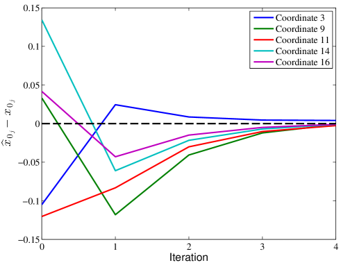
Figure 11: Error of the estimate $\widehat{x}_{0_{j}}^{(m)}$ (for five example coordinates) at iteration $m$ of Algorithm 1 for a “Baseline” data set (see Table 2) with $\tau_{j}\sim\mathcal{N}(0,\sigma^{2})$.

6 Discussion and Conclusion

6.1 Consistency with Previously Established Results

Local PCA of manifold-valued data has received attention in several recent works (for example, those referenced in Section 1). In particular, the analyses of Maggioni-long and Singer , after suitable translation of notation and assumptions, demonstrate growth rates for the PCA spectrum that match those computed in the present work. The focus of our analysis is the perturbation of the eigenspace recovered from the local data covariance matrix. We therefore confirm our results with those most similar from the literature. The most closely related results are those of Nadler , in which matrix perturbation theory is used to study the PCA spectrum; Tyagi , where neighborhood size and sampling conditions are given to ensure an accurate tangent space estimate from noise-free manifold-valued data; and Maggioni-MIT , where theory is developed for the implementation of multiscale PCA to detect the intrinsic dimension of a manifold.

In Nadler , a finite-sample PCA analysis assuming a linear model is presented. Keeping $N$ and $D$ fixed, the noise level $\sigma$ is considered to be a small parameter. Much like the analysis of the present paper, the results are derived in the non-asymptotic setting. However, the bound on the angle between the finite-sample and population eigenvectors is summarized in Nadler for the asymptotic regime where $N$ and $D$ become large. The result, restated here in our notation, takes the form:

$$\sin\theta_{\widehat{U}_{1},U_{1}}~{}\lesssim~{}\frac{\sigma}{\sqrt{\lambda_{d}}}\sqrt{\frac{D}{N}}+\mathcal{O}(\sigma^{2}).$$

We note that the main results of Nadler are stated for $N\leq D$ and that our analysis expects the opposite in general, although it is not explicitly required. Nonetheless, by setting curvature terms to zero, our results recover the reported leading behavior following the same asymptotic regime as Nadler , where terms $\mathcal{O}(1/\sqrt{N})$ are neglected and $\sigma$ is treated as a small parameter. After setting all curvature terms to zero, we assume condition 1 holds such that the denominator $\delta$ is sufficiently well conditioned and we may drop all terms other than $\lambda_{d}$. Then our Main Result has the form:

$$\sin\theta_{\widehat{U}_{1},U_{1}}~{}\lesssim~{}\frac{1}{\sqrt{N}}\frac{1}{\lambda_{d}}\sigma\sqrt{d(D-d)}\left[\frac{r}{\sqrt{d+2}}+\sigma\right]=\frac{\sigma}{\sqrt{\lambda_{d}}}\frac{\sqrt{d(D-d)}}{\sqrt{N}}+\mathcal{O}(\sigma^{2}).$$

Setting $d=1$ to match the analysis in Nadler recovers its curvature-free result.

Next, Tyagi presents an analysis of local PCA differing from ours in two crucial ways. First, the analysis of Tyagi does not include high-dimensional noise perturbation and the data points are assumed to be sampled directly from the manifold. Second, the sampling density is not fixed, whereas the neighborhood size determines the number of sample points in our analysis. In fact, a goal of the analysis in Tyagi is to determine a sampling density that will yield an accurate tangent space estimate.

Allowing for a variable sampling density has the effect of decoupling the condition number $\delta^{-1}$ from the norm $\|U_{2}^{T}\Delta U_{1}\|_{F}$ measuring the amount of “lift” in directions normal to the tangent space due to the perturbation. The analysis of Tyagi proceeds by first determining the optimal neighborhood radius $r^{*}$ in the asymptotic limit of infinite sampling, $N\rightarrow\infty$. This approach yields the requirement that the spectra associated with the tangent space and curvature be sufficiently separated. Translating to our notation, setting noise terms to zero, and assuming the asymptotic regime of Tyagi such that we may neglect finite-sample correction terms, we recover condition 1 of our Main Result Theorem 3.2:

$$\lambda_{d}-\|U_{2}^{T}\Delta U_{2}\|_{F}=\lambda_{d}-\|U_{2}^{T}\frac{1}{N}CC^{T}U_{2}\|_{F}>0.$$ (69)

Thus, Theorem 1 of Tyagi requires that $r$ be chosen such that the subspace recovery problem is well conditioned in the same sense that we require by condition 1. Substituting the expectations for each term in (69) yields

$$\frac{r^{2}}{(d+2)}-\frac{K^{2}r^{4}(d+1)}{2(d+2)^{2}(d+4)}>0,$$

implying the choice $r<c/K$ (for a constant $c>0$), in agreement with the analysis of Tyagi . Once the proper neighborhood size has been selected, the decoupling assumed in Tyagi allows a choice of sampling density large enough to ensure a small angle. Again translating to our result (29), once $r$ is selected so that the denominator $\delta$ is well conditioned, the density may be chosen such that the $1/\sqrt{N}$ decay of the numerator $\|U_{2}^{T}\Delta U_{1}\|_{F}$ allows for a small recovery angle. Thus, we see that in the limit of infinite sampling and absence of noise, our results are consistent with those of Tyagi in the fixed density setting.

Finally, the recent work Maggioni-MIT studies multiscale PCA and the growth of the corresponding spectrum to detect the intrinsic dimension of a manifold (or, more generally, a point cloud of random samples from a distribution concentrated around a low-dimensional manifold). The authors prove, under appropriate conditions, that the empirical covariance of noisy points localized in a Euclidean ball about a noisy center is close to the population covariance of the underlying distribution, with high probability. In particular, the authors’ very detailed analysis shows that one may estimate the population covariance from the empirical covariance of noisy points that are localized before noise is added. Then, following the work in LittleThesisDuke , further effort in Maggioni-MIT examines the effect of centering the multiscale analysis about a noisy origin.

Given an appropriate translation of the assumptions, the key results in Maggioni-MIT are of the same order as those in the present work. Using our notation, Maggioni-MIT proceeds with an analysis of the geometric terms contained in the covariance $\frac{1}{N}\widetilde{X}\widetilde{X}^{T}$ and bounds the difference from the population covariance by controlling the perturbation due to the noisy center and the localization process. In both the present analysis and that of Maggioni-MIT , the empirical covariance $\frac{1}{N}\widetilde{X}\widetilde{X}^{T}$, computed from points localized before adding noise, provides the leading order terms that drive the behavior of $\|P-\widehat{P}\|_{F}$. By moving the analysis from $r$ to $R$ in Section 5, we allow both curvature and noise to affect the localization of points and experimentally verify that $\|P-\widehat{P}\|_{F}$ is consistent with our Main Result. Indeed, the results in Section 5 experimentally test and confirm that the perturbation caused by such localization is small, as is theoretically derived in Maggioni-MIT . The effect of centering about a noisy origin is addressed in Maggioni-MIT through a rescaling of the observable radius, and conditions are given that allow for the covariance of the set of points localized about a noisy origin to be close to the covariance of the points localized about the true origin. The algorithm introduced in the present work, Algorithm 1 of Section 5, provides a simple method for recovering the true origin that may be used in practice. Through a very different framework than that of the analysis in Maggioni-MIT , our method uses the geometric information encoded in the center of mass to compute the true origin of the local neighborhood. Our results therefore offer an algorithmic companion to the analysis presented in Maggioni-MIT .

6.2 Algorithmic Considerations

6.2.1 Parameter Estimation

Practical methods must be developed to recover parameters such as dimension, curvature, and noise. Such parameters are necessary for any analysis or algorithm and should be recovered directly from the data rather than estimated by a priori fixed values. The experimental results presented above suggest the particular importance of accurately estimating the intrinsic dimension $d$, for which there exist several algorithms. Fukunaga introduced a local PCA-based approach for estimating $d$ in Fukunaga-Olsen . The recent work in Maggioni-long presents a multiscale approach that estimates $d$ in a pointwise fashion. Performing an SVD at each scale, $d$ is determined by examining growth rate of the multiscale singular values. It would be interesting to investigate if this approach remains robust if only a coarse exploration of the scales is performed, as it may be possible to reduce the computational cost through an SVD-update scheme. Another scale-based approach is presented in Wang-Marron and the problem was studied from a dynamical systems perspective in Froehling .

There exist statistical methods for estimating the noise level present in a data set that should be useful in the context of this work (see, for example, Broomhead ; Donoho2 ). We experimentally obtain a reliable estimate of the noise level from the median of the smallest singular values over several small neighborhoods (results not shown). In Maggioni-long , the smallest multiscale singular values are used as an estimate for the noise level and a scale-dependent estimate of noise variance is suggested in Jones-new for curve-denoising. Methods for estimating curvature (e.g., Williams-curvature ; Kresk-curvature ) have been developed for application to computer vision and extensions to the high-dimensional setting should be explored. Further, if one is willing to perform many SVDs of large matrices, our method of tracking the center of mass presented in Section 5 combined with the growth rates for the PCA spectrum presented in Maggioni-long might yield the individual principal curvatures.

6.2.2 Sampling

For a tractable analysis, assumptions about sampling must be made. In this work we have assumed uniform sampling in the tangent plane. This is merely one choice and we have conducted initial experiments uniformly sampling the manifold rather than the tangent plane. Results suggest that for a given radius, sampling the manifold yields a smaller curvature perturbation than that from sampling the tangent plane. While more rigorous analysis and experimentation is needed, it is clear that consideration must be given to the sampling assumptions for any practical algorithm.

6.2.3 From Tangent Plane Recovery to Data Parameterization

The tangent plane recovered by our approach may not provide the best approximation over the entire neighborhood from which it was derived. Depending on a user-defined error tolerance, a smaller or larger sized neighborhood may be parameterized by the local chart. If high accuracy is required, one might only parameterize a neighborhood of size $N<N^{*}$ to ensure the accuracy requirement is met. Similarly, if an application requires only modest accuracy, one may be able to parameterize a larger neighborhood than that given by $N^{*}$.

Finally, we may wish to use tangent planes recovered from different neighborhoods to construct a covering of a data set. There exist methods for aligning local charts into a global coordinate system (for example Brand ; Roweis-Global ; Zhang-Zha , to name a few). Care should be taken to define neighborhoods such that a data set may be optimally covered.

Funding

This work was supported by the National Science Foundation [DMS-0941476 to F.G.M. and D.N.K., ACI-1226362 and DGE-0801680 to D.N.K.]; and the Department of Energy [DE-SC0004096 to F.G.M.].

Appendix

Technical calculations are presented in this appendix. In particular, the norm of each random matrix contributing to the perturbation term $\Delta$, defined in equation (18), is bounded with high probability. The analysis is divided between three cases: (1) norms of products of bounded random matrices; (2) norms of products of unbounded random matrices; and (3) norms of products of bounded and unbounded random matrices.

Each case requires careful attention to derive a tight result that avoids large union bounds and ensures high probability that is independent of the ambient dimension $D$. The analysis proceeds by bounding the eigenvalues of the covariance matrices of $(L-\overline{L})$, $(C-\overline{C})$, and $(E-\overline{E})$ using results from random matrix theory and properties of the spectral norm. A detailed analysis of each of the three cases follows.

Before we start the proofs, one last comment is in order. The reader will notice that we sometimes introduce benign assumptions about the number of samples $N$ or the dimensions $d$ or $D$ in order to provide bounds that are simpler to interpret. These assumptions are not needed to derive any of the results; they are merely introduced to help us simplify a complicated expression, and introduce upper bounds that hold under these fairly benign assumptions. This should help the reader interpret the size of the different terms.

Notation

We often vectorize matrices by concatenating the columns of a matrix. If $M=[m^{(1)}|\cdots|m^{(N)}]$, then we define

$$\overrightarrow{m}=\text{vec}\left(M\right)=\begin{bmatrix}m^{(1)}\\ \vdots\\ m^{(N)}\end{bmatrix}.$$

We denote the largest and smallest eigenvalue of a square matrix $M$ by

$$\lambda_{\max}(M)\quad\text{and}\quad\lambda_{\min}(M),$$

respectively. In the main body of the paper, we use the standard notation $\overline{X}$ to denote the sample mean of $N$ columns from the matrix $X$. In this appendix, we introduce a second notation to denote the same concept,

$$\widehat{\operatorname{\mathbb{E}}}[X]=\overline{X}=\frac{1}{N}\sum_{n=1}^{N}x^{(n)}.$$

Finally, we denote by $\operatorname{\mathbb{E}}[X]$ the expectation of the random matrix $X$ and by the probability of event $\mathscr{E}$.

Appendix A Eigenvalue Bounds

A.1 Linear Eigenvalues

We seek a bound on the maximum and minimum (nonzero) eigenvalue of the matrix

$$\frac{1}{N}(L-\overline{L})(L-\overline{L})^{T}=\frac{1}{N}\sum_{k=1}^{N}(\ell^{(k)}-\overline{\ell})(\ell^{(k)}-\overline{\ell})^{T}.$$ (70)

As only the nonzero eigenvalues are of interest, we proceed by considering only the nonzero upper-left $d\times d$ block of the matrix in (70), or equivalently, by ignoring the trailing zeros of each realization $\ell^{(k)}$. Thus, momentarily abusing notation, we consider the matrix in (70) to be of dimension $d\times d$. The analysis utilizes the following theorem found in Tropp .

Theorem A.1 (Matrix Chernoff II, Tropp ).

Consider a finite sequence $\{X_{k}\}$ of independent, random, self adjoint matrices that satisfy

$$X_{k}\succcurlyeq 0\qquad\text{and}\qquad\lambda_{\max}(X_{k})\leq\lambda_{\infty}\quad\text{almost surely}.$$

Compute the minimum and maximum eigenvalues of the sum of expectations,

$$\mu_{\min}:=\lambda_{\min}\left(\sum_{k=1}^{N}\operatorname{\mathbb{E}}{\color[rgb]{0,0,0}[}X_{k}{\color[rgb]{0,0,0}]}\right)\quad\text{and}\quad\mu_{\max}:=\lambda_{\max}\left(\sum_{k=1}^{N}\operatorname{\mathbb{E}}{\color[rgb]{0,0,0}[}X_{k}{\color[rgb]{0,0,0}]}\right).$$

Then

$$\mathbb{P}\left[\lambda_{\min}\left(\sum_{k=1}^{N}X_{k}\right)\leq(1-\delta)\mu_{\min}\right]\leq d\left[\frac{e^{-\delta}}{(1-\delta)^{(1-\delta)}}\right]^{\mu_{\min}/\lambda_{\infty}},\quad\text{for }\delta\in[0,1],\text{ and}$$

$$\mathbb{P}\left[\lambda_{\max}\left(\sum_{k=1}^{N}X_{k}\right)\geq(1+\delta)\mu_{\max}\right]\leq d\left[\frac{e^{\delta}}{(1+\delta)^{(1+\delta)}}\right]^{\mu_{\max}/\lambda_{\infty}},\quad\text{for }\delta\geq 0.$$

We apply this result to

$$X_{k}=\frac{1}{N}(\ell^{(k)}-\overline{\ell})(\ell^{(k)}-\overline{\ell})^{T}.$$

Clearly $X_{k}$ is a symmetric positive semi-definite matrix and we have $X_{k}\succcurlyeq 0$. Next,

$$\lambda_{\max}(X_{k})=\left\|\frac{1}{N}(\ell^{(k)}-\overline{\ell})(\ell^{(k)}-\overline{\ell})^{T}\right\|_{2}{\color[rgb]{0,0,0}=}\frac{1}{N}\left\|\ell^{(k)}-\overline{\ell}\right\|^{2}\leq\frac{1}{N}\left(\|\ell\|+\|\overline{\ell}\|\right)^{2}\leq\frac{4r^{2}}{N}$$

and we set $\lambda_{\infty}=4r^{2}/N$. Simple computations yield

$$\lambda_{\max}\left(\sum_{k=1}^{N}\operatorname{\mathbb{E}}[X_{k}]\right)=\frac{r^{2}}{d+2}\left[1-\frac{1}{N}\right]^{2},\quad\text{and}\quad\lambda_{\min}\left(\sum_{k=1}^{N}\operatorname{\mathbb{E}}[X_{k}]\right)=\frac{r^{2}}{d+2}\left[1-\frac{1}{N}\right]^{2},$$

and we set

$$\mu_{\max}=\mu_{\min}=\mu=\frac{r^{2}}{d+2}\left[1-\frac{1}{N}\right]^{2}.$$

By Theorem A.1 and using standard manipulations, we have the following result bound for the smallest eigenvalue, $\lambda_{d}$ in our notation,

$$\lambda_{d}>\frac{r^{2}}{d+2}\left[1-\frac{1}{N}\right]^{2}\left[1-\xi_{\lambda_{d}}\frac{1}{\sqrt{N}}\frac{\sqrt{8(d+2)}}{(1-\frac{1}{N})}\right]$$

with probability greater than $1-de^{-\xi_{\lambda_{d}}^{2}}$. Similarly, the following result holds for the largest eigenvalue, $\lambda_{1}$ in our notation:

$$\lambda_{1}\leq\frac{r^{2}}{d+2}\left[1+\xi_{\lambda_{1}}\frac{5\sqrt{d+2}}{\sqrt{N}}\right]$$ (71)

with probability greater than $1-de^{-\xi_{\lambda_{1}}^{2}}$, as soon as $N>3$. We define the last upper bound as

$$\lambda_{\text{bound}}(\xi)=\frac{r^{2}}{d+2}\left[1+\xi\frac{5\sqrt{d+2}}{\sqrt{N}}\right],$$ (72)

and we can use this bound to control the size of all the eigenvalues of the matrix $\frac{1}{N}(L-\overline{L})(L-\overline{L})^{T}$,

(73)

Now that we have computed the necessary bounds for all nonzero linear eigenvalues, we return to our standard notation for the remainder of the analysis: each $\ell^{(k)}$ is of length $D$ with $\ell_{j}^{(k)}=0$ for $d+1\leq j\leq D$ and $L=[\ell^{(1)}|\ell^{(2)}|\cdots|\ell^{(N)}]$ is a $D\times N$ matrix.

A.2 Curvature Eigenvalues

To bound the largest eigenvalue, $\gamma_{1}$, of $\frac{1}{N}(C-\overline{C})(C-\overline{C})^{T}$ we note that the spectral norm is bounded by the Frobenius norm and we use the bound on the Frobenius norm derived in Section B.1. We can use this bound to control the size of all the eigenvalues of the matrix $\frac{1}{N}(C-\overline{C})(C-\overline{C})^{T}$,

(74)

where

$$\gamma_{\text{bound}}(\xi)=\frac{r^{4}}{2(d+4)(d+2)^{2}}\sqrt{\sum_{i,j=d+1}^{D}\negthickspace\negthickspace[(d+1)K_{nn}^{ij}-K_{mn}^{ij}]^{2}}+\frac{(K^{(+)})^{2}r^{4}}{4\sqrt{N}}\left[(2+\xi\sqrt{2})+\frac{(2+\xi\sqrt{2})^{2}}{\sqrt{N}}\right].$$ (75)

The proof of the bound on the Frobenius norm is delayed until Section B.1.

Remark A.2.

A different (possibly tighter) bound may be derived using Theorem A.1. However, such a bound would hold with a probability that becomes small when the ambient dimension $D$ is large. We therefore proceed with the bound (75) above, noting that we sacrifice no additional probability by using it here since it is required for the analysis in Section B.1.

A.3 Noise Eigenvalues

We may control the eigenvalues of $\frac{1}{N}(E-\overline{E})(E-\overline{E})^{T}$ using standard results from random matrix theory. In particular, let $s_{\min}(E)$ and $s_{\max}(E)$ denote the smallest and largest singular value of matrix $E$, respectively. The following result (Corollary 5.35 of Vershynin ) gives a tight control on the size of $s_{\min}(E)$ and $s_{\max}(E)$ when $E$ has Gaussian entries.

Theorem A.3 (Vershynin ; Edelman88 ).

Let $A$ be a $D\times N$ matrix whose entries are independent standard normal random variables. Then for every $t\geq 0$, with probability at least $1-2\exp(-t^{2}/2)$ one has

$$\sqrt{N}-\sqrt{D}-t~{}\leq~{}s_{\min}(A)~{}\leq~{}s_{\max}(A)~{}\leq~{}\sqrt{N}+\sqrt{D}+t.$$ (76)

Define

$$\alpha=\left(\sigma\sqrt{1-\frac{1}{N}}\right)^{-1}$$ (77)

and note that the entries of $Z=\alpha(E-\overline{E})$ are independent standard normal random variables. This normalization by $\alpha$ allows us to use Theorem A.3 and we divide by $\alpha^{2}$ to recover the result for $(E-\overline{E})(E-\overline{E})^{T}$. Let us partition the Gaussian vector $e$ into the first $d$ coordinates, $e_{1}$, and last $D-d$ coordinates, $e_{2}$,

$$e=\begin{bmatrix}e_{1}&|&e_{2}\end{bmatrix}^{T},$$ (78)

and observe that the matrix $U_{1}^{T}\frac{1}{N}(E-\overline{E})(E-\overline{E}^{T})U_{1}$ only depends on the realizations of $e_{1}$. Similarly, the matrix $U_{2}^{T}\frac{1}{N}(E-\overline{E})(E-\overline{E}^{T})U_{2}$ only depends on the realizations of $e_{2}$. By Theorem A.3, we have

$$\lambda_{\max}\left(\frac{1}{N}U_{1}^{T}(E-\overline{E})(E-\overline{E}^{T})U_{1}\right)\leq{\color[rgb]{0,0,0}\sigma^{2}\left(1+\frac{5}{2\sqrt{N}}(\sqrt{d}+\xi_{e_{1}})\right)}$$ (79)

with probability at least $1-e^{-\xi_{e_{1}}^{2}}$ over the random realization of $e_{1}$, as soon as $N>4(\sqrt{d}+\xi_{e_{1}})$, a condition easily satisfied for any reasonable sampling density. Similarly,

$$\lambda_{\max}\left(\frac{1}{N}U_{2}^{T}(E-\overline{E})(E-\overline{E}^{T})U_{2}\right)\leq{\color[rgb]{0,0,0}\sigma^{2}\left(1+\frac{5}{2\sqrt{N}}(\sqrt{D-d}+\xi_{e_{2}})\right)}$$ (80)

with probability at least $1-e^{-\xi_{e_{2}}^{2}}$ over the random realization of $e_{2}$, as soon as $N>4(\sqrt{D-d}+\xi_{e_{2}})$.

Appendix B Products of Bounded Random Matrices

B.1 Curvature Term: $CC^{T}$

Begin by recalling the notation used for the curvature constants,

$$K_{i}=\sum_{n=1}^{d}\kappa_{n}^{(i)},\quad K=\left(\sum_{i=d+1}^{D}K_{i}^{2}\right)^{\frac{1}{2}}\negthickspace,\quad K_{nn}^{ij}=\sum_{n=1}^{d}\kappa_{n}^{(i)}\kappa_{n}^{(j)},\quad K_{mn}^{ij}=\sum_{\begin{subarray}{c}m,n=1\\ m\neq n\end{subarray}}^{d}\kappa_{m}^{(i)}\kappa_{n}^{(j)}.$$ (81)

The constant $K_{i}$ quantifies the curvature in normal direction $i$, for $i=(d+1),$ $\dots,D$. The overall compounded curvature of the local model is quantified by $K$ and is a natural result of our use of the Frobenius norm. We note that $K_{i}K_{j}=K_{nn}^{ij}+K_{mn}^{ij}$. We also recall the positive constants

$$K_{i}^{(+)}=\left(\sum_{n=1}^{d}|\kappa_{n}^{(i)}|^{2}\right)^{\frac{1}{2}},\quad\text{and}\quad K^{(+)}=\left(\sum_{i=d+1}^{D}(K_{i}^{(+)})^{2}\right)^{\frac{1}{2}}.$$ (82)

Our strategy for bounding the matrix norm $\|U_{2}^{T}\frac{1}{N}(C-\overline{C})(C-\overline{C})^{T}U_{2}\|_{F}$ begins with the observation that $\frac{1}{N}(C-\overline{C})(C-\overline{C})^{T}$ is a sample mean of $N$ covariance matrices of the vectors $(c^{(k)}-\overline{c})$, $k=1,\dots,N$. That is,

$$\frac{1}{N}(C-\overline{C})(C-\overline{C})^{T}=\widehat{\operatorname{\mathbb{E}}}[(c-\widehat{\operatorname{\mathbb{E}}}[c])(c-\widehat{\operatorname{\mathbb{E}}}[c])^{T}].$$ (83)

We therefore expect that $\frac{1}{N}(C-\overline{C})(C-\overline{C})^{T}$ converges toward the centered covariance matrix of $c$. We will use the following result of Shawe-Taylor and Cristianini shawe to bound, with high probability, the norm of the difference between this sample mean and its expectation.

Theorem B.1.

(Shawe-Taylor & Cristianini, shawe ). Given $N$ realizations of a random matrix $Y$ distributed with probability distribution , we have

(84)

The constant $R=\sup_{\begin{subarray}{c}\text{supp}(\prob{}_{Y})\end{subarray}}\|Y\|_{F}$, where supp$($ is the support of distribution .

We note that the original formulation of the result involves only random vectors, but since the Frobenius norm of a matrix is merely the Euclidean norm of its vectorized version, we formulate the theorem in terms of matrices. We also note that the choice of $R$ in (LABEL:eq:shawe-taylor) need not be unique. Our analysis will proceed by using upper bounds for $\|Y\|_{F}$ which may not be suprema. Let

$$R_{c}=\sup_{{\color[rgb]{0,0,0}c}}\|U_{2}^{T}c\|_{F}.$$

Using Theorem B.1 and modifying slightly the proof of Corollary 6 in shawe , which uses standard inequalities, we arrive at

$$\bigg{|}\left\|\operatorname{\mathbb{E}}[U_{2}^{T}(c-\operatorname{\mathbb{E}}[c])(c-\operatorname{\mathbb{E}}[c])^{T}U_{2}]\right\|_{F}-\left\|\widehat{\operatorname{\mathbb{E}}}[U_{2}^{T}(c-\widehat{\operatorname{\mathbb{E}}}[c])(c-\widehat{\operatorname{\mathbb{E}}}[c])^{T}U_{2}]\right\|_{F}\bigg{|}$$

$$\leq\left\|\operatorname{\mathbb{E}}[U_{2}^{T}cc^{T}U_{2}]-\widehat{\operatorname{\mathbb{E}}}[U_{2}^{T}cc^{T}U_{2}]\right\|_{F}\negthickspace+\left\|\operatorname{\mathbb{E}}[U_{2}^{T}c]-\widehat{\operatorname{\mathbb{E}}}[U_{2}^{T}c]\right\|_{F}^{2}\leq\frac{R_{c}^{2}}{\sqrt{N}}\left(2+\xi_{c}\sqrt{2}\right) +\frac{R_{c}^{2}}{N}\left(2+\xi_{c}\sqrt{2}\right)^{2}$$

with probability greater than $1-2e^{-\xi_{c}^{2}}$ over the random selection of the sample points. To complete the bound we must compute $R_{c}$ and $\left\|\operatorname{\mathbb{E}}[U_{2}^{T}(c-\operatorname{\mathbb{E}}[c])(c-\operatorname{\mathbb{E}}[c])^{T}U_{2}]\right\|_{F}$. A simple norm calculation shows

$$\|U_{2}^{T}c\|_{F}^{2}=\frac{1}{4}\sum_{i=d+1}^{D}\left(\kappa_{1}^{(i)}\ell_{1}^{2}+~{}\dots~{}+\kappa_{d}^{(i)}\ell_{d}^{2}\right)^{2}\leq\frac{r^{4}}{4}\sum_{i=d+1}^{D}\left(K_{i}^{(+)}\right)^{2}=\frac{(K^{(+)})^{2}r^{4}}{4},$$

and we set $R_{c}=K^{(+)}r^{2}/2$. Next, the expectation takes the form

$$\Big{\|}\operatorname{\mathbb{E}}[U_{2}^{T}(c-\operatorname{\mathbb{E}}[c])(c-\operatorname{\mathbb{E}}[c])^{T}U_{2}]\Big{\|}_{F}~{}=~{}\Big{\|}\operatorname{\mathbb{E}}[U_{2}^{T}cc^{T}U_{2}]-\operatorname{\mathbb{E}}[U_{2}^{T}c]\operatorname{\mathbb{E}}[c^{T}U_{2}]\Big{\|}_{F}.$$

We calculate

$$\operatorname{\mathbb{E}}[c_{i}c_{j}]=\frac{\left[3K_{nn}^{ij}+K_{mn}^{ij}\right]r^{4}}{4(d+2)(d+4)},\quad\text{and}\quad\operatorname{\mathbb{E}}[c_{i}]\operatorname{\mathbb{E}}[c_{j}]=\frac{\left[K_{nn}^{ij}+K_{mn}^{ij}\right]r^{4}}{4(d+2)^{2}}$$

and compute the norm

$$\Big{\|}\operatorname{\mathbb{E}}[U_{2}^{T}(c-\operatorname{\mathbb{E}}[c])(c-\operatorname{\mathbb{E}}[c])^{T}U_{2}]\Big{\|}_{F}=\frac{r^{4}}{2(d+2)^{2}(d+4)}\sqrt{\sum_{i,j=d+1}^{D}\left[(d+1)K_{nn}^{ij}-K_{mn}^{ij}\right]^{2}}.$$

Finally, putting it all together, we conclude that

$$\left\|U_{2}^{T}\frac{1}{N}(C-\overline{C})(C-\overline{C})^{T}U_{2}\right\|_{F}\leq~{} \frac{r^{4}}{2(d+2)^{2}(d+4)}\sqrt{\sum_{i,j=d+1}^{D}\left[(d+1)K_{nn}^{ij}-K_{mn}^{ij}\right]^{2}}$$

$$+\frac{1}{\sqrt{N}}\frac{(K^{(+)})^{2}r^{4}}{4}\left[\left(2+\xi_{c}\sqrt{2}\right)+\frac{1}{\sqrt{N}}\left(2+\xi_{c}\sqrt{2}\right)^{2}\right]$$

with probability greater than $1-2e^{-\xi_{c}^{2}}$ over the random selection of the sample points.

B.2 Curvature-Linear Cross-Terms: $CL^{T}$

Our approach for bounding the matrix norm $\|U_{2}^{T}\frac{1}{N}(C-\overline{C})(L-\overline{L})^{T}U_{1}\|_{F}$ mirrors that of Section B.1. Here, we use that $\operatorname{\mathbb{E}}[\ell_{i}]=0$ for $1\leq i\leq d$ and proceed as follows. We have

$$R_{\ell}=\sup_{\ell}\|\ell^{T}U_{1}\|_{F}=r.$$

Reasoning as in the previous section, we have

$$\bigg{|}\left\|\operatorname{\mathbb{E}}[U_{2}^{T}(c-\operatorname{\mathbb{E}}[c])(\ell-\operatorname{\mathbb{E}}[\ell])^{T}U_{1}]\right\|_{F}-\left\|\widehat{\operatorname{\mathbb{E}}}[U_{2}^{T}(c-\widehat{\operatorname{\mathbb{E}}}[c])(\ell-\widehat{\operatorname{\mathbb{E}}}[\ell])^{T}U_{1}]\right\|_{F}\bigg{|}$$

$$\leq\left\|\operatorname{\mathbb{E}}[U_{2}^{T}c\ell^{T}U_{1}]-\widehat{\operatorname{\mathbb{E}}}[U_{2}^{T}c\ell^{T}U_{1}]\right\|_{F}+\left\|\widehat{\operatorname{\mathbb{E}}}[\ell^{T}U_{1}]-\operatorname{\mathbb{E}}[\ell^{T}U_{1}]\right\|_{F}\bigg{(}\left\|\widehat{\operatorname{\mathbb{E}}}[U_{2}^{T}c]-\operatorname{\mathbb{E}}[U_{2}^{T}c]\right\|_{F}+ \left\|\operatorname{\mathbb{E}}[U_{2}^{T}c]\right\|_{F}\bigg{)}$$

$$\leq\frac{R_{c}R_{\ell}}{\sqrt{N}}\left(2+\xi_{c\ell}\sqrt{2}\right)+\frac{R_{\ell}}{\sqrt{N}}\left(2+\xi_{\ell}\sqrt{2}\right)\bigg{[}\frac{R_{c}}{\sqrt{N}}\left(2+\xi_{c}\sqrt{2}\right)+\left\|\operatorname{\mathbb{E}}[U_{2}^{T}c]\right\|_{F}\bigg{]}$$

with probability greater than $1-e^{-\xi_{c\ell}^{2}}-e^{-\xi_{\ell}^{2}}-e^{-\xi_{c}^{2}}$ over the random selection of the sample points. Finally, we set $\xi_{\ell}=\xi_{c\ell}$ and conclude

$$\left\|U_{2}^{T}\frac{1}{N}(C-\overline{C})(L-\overline{L})^{T}U_{1}\right\|_{F}\leq\frac{K^{(+)}r^{3}}{2\sqrt{N}}\left[\frac{d+3}{d+2}\left(2+\xi_{c\ell}\sqrt{2}\right)+\frac{1}{\sqrt{N}}\left(2+\xi_{c}\sqrt{2}\right)\left(2+\xi_{c\ell}\sqrt{2}\right)\right]$$

with probability greater than $1-2e^{-\xi_{c\ell}^{2}}-e^{-\xi_{c}^{2}}$ over the random selection of the sample points.

Appendix C Products of Unbounded Random Matrices: $EE^{T}$

We seek bounds for the matrix norms of the form

$$\left\|U_{n}^{T}\frac{1}{N}(E-\overline{E})(E-\overline{E})^{T}U_{m}\right\|_{F}\quad\text{for $(n,m)=(1,1),(2,2)$, and $(2,1)$}.$$ (85)

Because $E$ is composed of $N$ columns of independent realizations of a $D$-dimensional Gaussian vector, the matrix $A$ defined by

$$A=\frac{1}{N-1}\frac{1}{\sigma^{2}}(E-\overline{E})(E-\overline{E})^{T}=\frac{\alpha^{2}}{N}(E-\overline{E})(E-\overline{E})^{T}$$

is Wishart $W_{D}\left(N-1,\frac{1}{N-1}I_{D}\right)$, where $\alpha=\left(\sigma\sqrt{1-\frac{1}{N}}\right)^{-1}\negthickspace$. As a result, we can quickly compute bounds on the terms (85) since they can be expressed as the norm of blocks of $A$. Indeed, let us partition $A$ as follows

$$A=\begin{bmatrix}A_{11}&A_{12}\\ A_{21}&A_{22}\end{bmatrix},$$

where $A_{11}$ is $d\times d$, $A_{22}$ is $(D-d)\times(D-d)$. We now observe that $A_{nm}$ is not equal to $\frac{\alpha^{2}}{N}U_{n}^{T}(E-\overline{E})(E-\overline{E})^{T}U_{m}$, but both matrices have the same Frobenius norm. Precisely, the two matrices differ only by a left and a right rotation, as explained in the next few lines.

Since only the first $d$ entries of each column in $U_{1}$ are nonzero, we can define two matrices $P_{1}$ and $Q_{1}$ that extract the first $d$ entries and apply the rotation associated with $U_{1}$, respectively, as follows

$$U_{1}=\begin{bmatrix}&&\\ &Q_{1}&\\ &&\\ 0&&0\\ \vdots&&\vdots\\ 0&&0\end{bmatrix}=\begin{bmatrix}1&&0\\ &\diagdown&\\ 0&&1\\ 0&&0\\ \vdots&&\vdots\\ 0&&0\end{bmatrix}Q_{1}=P_{1}Q_{1}.$$

We define similar matrices $P_{2}$ and $Q_{2}$ such that $U_{2}=P_{2}Q_{2}$. We conclude that

$$\left\|U_{n}^{T}(E-\overline{E})(E-\overline{E})^{T}U_{m}\right\|_{F}=\left\|P_{n}^{T}(E-\overline{E})(E-\overline{E})^{T}P_{m}\right\|_{F}=\frac{N}{\alpha^{2}}\left\|A_{nm}\right\|_{F}.$$

In summary, we can control the size of the norms (85) by controlling the norm of the sub-matrices of a Wishart matrix. We first estimate the size of $\|A_{11}\|_{F}$ and $\|A_{22}\|_{F}$. This is a straightforward affair, since we can apply Theorem A.3 with $P_{1}{\color[rgb]{0,0,0}(E-\overline{E})}$ and $P_{2}{\color[rgb]{0,0,0}(E-\overline{E})}$, respectively, to get the spectral norm of $A_{11}$ and $A_{22}$. We then apply a standard inequality between the spectral and the Frobenius norm of a matrix $M$,

$$\|M\|_{F}\leq\sqrt{\text{rank}\left(M\right)}\|M\|_{2}.$$ (86)

This bound is usually quite loose and equality is achieved only for the case where all singular values of matrix $A$ are equal. It turns out that this special case holds in expectation for the matrices in the analysis to follow, and thus (86) provides a tight estimate of the Frobenius norm. Using (79) and (86), we have the following bound

$$\left\|U_{1}^{T}\frac{1}{N}(E-\overline{E})(E-\overline{E})^{T}U_{1}\right\|_{F}\leq\sigma^{2}\sqrt{d}\left[1+\frac{5}{2}\frac{1}{\sqrt{N}}(\sqrt{d}+\xi_{e_{1}}\sqrt{2})\right]$$

with probability greater than $1-e^{-\xi_{e_{1}}^{2}}$ over the random realization of the noise. By (80), we also have

$$\left\|U_{2}^{T}\frac{1}{N}(E-\overline{E})(E-\overline{E})^{T}U_{2}\right\|_{F}\leq\sigma^{2}\sqrt{D-d}\left[1+\frac{5}{2}\frac{1}{\sqrt{N}}(\sqrt{D-d}+\xi_{e_{2}}\sqrt{2})\right]$$

with probability greater than $1-e^{-\xi_{e_{2}}^{2}}$ over the random realization of the noise.

It remains to bound $\|A_{21}\|$. Here we proceed by conditioning on the realization of the last $D-d$ coordinates of the noise vectors in the matrix $E$; in other words, we freeze $P_{2}E$. Rather than working with Gaussian matrices, we prefer to vectorize the matrix $A_{21}$ and define

$$\overrightarrow{a_{21}}=\text{vec}\left(A^{T}_{21}\right).$$

Note that here we unroll the matrix $A_{21}$ row by row to build $\overrightarrow{a_{21}}$. Because the Frobenius norm of $A_{21}$ is the Euclidean norm of $\overrightarrow{a_{21}}$, we need to find a bound on $\|\overrightarrow{a_{21}}\|$. Conditioning on the realization of $P_{2}E$, we know (Theorem 3.2.10 of Muirhead ) that the distribution of $\overrightarrow{a_{21}}$ is a multivariate Gaussian variable $\mathcal{N}(\overrightarrow{0},S)$, where $\overrightarrow{0}$ is the zero vector of dimension $d(D-d)$ and $S$ is the $d(D-d)\times d(D-d)$ block diagonal matrix containing $d$ copies of $\frac{1}{N}A_{22}$

$$S=\frac{1}{N}\begin{bmatrix}A_{22}&&&\\ &A_{22}&&\\ &&\ddots&\\ &&&A_{22}\end{bmatrix}.$$

Let $S^{\dagger}$ be a generalized inverse of $S$ (such that $SS^{\dagger}S=S$), then (see e.g. Theorem 1.4.4 of Muirhead )

$$\overrightarrow{a_{21}}^{T}S^{\dagger}\overrightarrow{a_{21}}\sim\chi^{2}(\text{rank}\left(S\right)).$$

Now, using only the bound for the smallest singular value in Theorem A.3, $A_{22}$ has full rank, $(D-d)$, with probability $1-e^{-(\sqrt{N}-\sqrt{D-d})^{2}/2}$, and therefore $S$ has full rank, $d(D-d)$, with the same probability. In the following, we derive an upper bound on the size of $\|\overrightarrow{a_{21}}\|$ when $A_{22}$ has full rank. A similar – but tighter – bound can be derived when $S$ is rank deficient; we only need to replace $(D-d)$ by the rank of $A_{22}$ in the bound that follows. Because the bound derived when $A_{22}$ is full rank will hold when $A_{22}$ is rank deficient (an event which happens with very small probability, anyway), we only worry about this case in the following. In this case, $S^{\dagger}=S^{-1}$ and

$$\overrightarrow{a_{21}}^{T}S^{-1}\overrightarrow{a_{21}}\sim\chi^{2}(d(D-d)).$$

Finally, using a corollary of Laurant and Massart (immediately following Lemma 1 of LaurantMassart ), we get that,

$$\overrightarrow{a_{21}}^{T}S^{-1}\overrightarrow{a_{21}}\leq d(D-d)+2\xi_{e_{3}}\sqrt{d(D-d)}+2\xi_{e_{3}}^{2}$$ (87)

with probability greater than $1-e^{-\xi_{e_{3}}^{2}}$. In the following, we assume that $\xi_{e_{3}}\leq 0.7\sqrt{d(D-d)}$, which happens as soon as $d$ or $D$ have a moderate size. Under this mild assumption we have

$$\sqrt{d(D-d)+2\xi_{e_{3}}\sqrt{d(D-d)}+2\xi_{e_{3}}^{2}}\leq\sqrt{d(D-d)}\left(1+\frac{6}{5}\frac{\xi_{e_{3}}}{\sqrt{d(D-d)}}\right).$$

In order to compare $\|\overrightarrow{a_{21}}\|^{2}$ to $\overrightarrow{a_{21}}^{T}S^{-1}\overrightarrow{a_{21}}$, we compute the eigendecomposition of $S$,

$$S=O~{}\varPi~{}O^{T},$$

where $O$ is a unitary matrix and $\varPi$ contains the eigenvalues of $\frac{1}{N}A_{22}$, repeated $d$ times. Letting $\lambda_{\max}\left(\frac{1}{N}A_{22}\right)$ be the largest eigenvalue of $\frac{1}{N}A_{22}$, we get the following upper bound,

$$\|\overrightarrow{a_{21}}\|^{2}\leq\lambda_{\max}\left(\frac{1}{N}A_{22}\right)\overrightarrow{a_{21}}^{T}\;O^{T}\varPi^{-1}O\;\overrightarrow{a_{21}}=\lambda_{\max}\left(\frac{1}{N}A_{22}\right)\overrightarrow{a_{21}}^{T}S^{-1}\overrightarrow{a_{21}}.$$

We conclude that, conditioned on a realization of the last $D-d$ entries of $E$, we have

(88)

To derive a bound on $\|\overrightarrow{a_{21}}\|$ that holds with high probability, we consider the event

$$\mathscr{E}_{\varepsilon,\xi}=\left\{\|\overrightarrow{a_{21}}\|\leq\frac{\sqrt{d(D-d)}}{\sqrt{N}}\left(1+\frac{\sqrt{D-d}+\varepsilon}{\sqrt{N}}\right)\left[1+\frac{6}{5}\frac{\xi}{\sqrt{d(D-d)}}\right]\right\}.$$

As we will see in the following, the event $\mathscr{E}_{\varepsilon,\xi}$ happens with high probability. This event depends on the random realization of the top $d$ coordinates, $e_{1}$, of the Gaussian vector $e$ (see (78)). Let us define a second likely event, which depends only on $e_{2}$ (the last $D-d$ coordinates of $e$),

$$\mathscr{E}_{e_{2}}=\left\{\sqrt{\lambda_{\max}\left(\frac{1}{N}A_{22}\right)}\leq\frac{1}{\sqrt{N}}\left(1+\frac{\sqrt{D-d}+\varepsilon}{\sqrt{N}}\right)\right\}.$$

Theorem A.3 tells us that the event $\mathscr{E}_{e_{2}}$ is very likely, and . We now show that the probability of $\mathscr{E}_{\varepsilon,\xi}^{c}$ is also very small,

Problem 11

In order to bound the first term, we condition on $e_{2}$,

Problem 16

Now the two conditions,

$$\begin{cases}\|\overrightarrow{a_{21}}\|>\sqrt{d(D-d)}\frac{1}{\sqrt{N}}\left(1+\frac{\sqrt{D-d}+\varepsilon}{\sqrt{N}}\right)\left[1+\frac{6}{5}\frac{\xi}{\sqrt{d(D-d)}}\right]\\ \frac{1}{\sqrt{N}}\left(1+\frac{\sqrt{D-d}+\varepsilon}{\sqrt{N}}\right)\geq\sqrt{\lambda_{\max}\left(\frac{1}{N}A_{22}\right)}\end{cases}$$

imply that

$$\|\overrightarrow{a_{21}}\|>\sqrt{d(D-d)}\sqrt{\lambda_{\max}\left(\frac{1}{N}A_{22}\right)}\left[1+\frac{6}{5}\frac{\xi}{\sqrt{d(D-d)}}\right],$$

and thus

Problem 18

Because of (LABEL:conditioned-wishart) the probability on the right-hand side is less than $e^{-\xi^{2}}$, which does not depend on $e_{2}$. We conclude that

Problem 20

Finally, since

$$\left\|U_{2}^{T}\frac{1}{N}(E-\overline{E})(E-\overline{E})^{T}U_{1}\right\|_{F}=\sigma^{2}\left(1-\frac{1}{N}\right)\|A_{21}\|_{F}=\sigma^{2}\left(1-\frac{1}{N}\right)\|\overrightarrow{a_{21}}\|,$$

we have

$$\left\|\frac{1}{N}U_{2}^{T}(E-\overline{E})(E-\overline{E})^{T}U_{1}\right\|_{F}\leq\frac{\sigma^{2}\sqrt{d(D-d)}}{\sqrt{N}}\left(\negthinspace 1+\frac{\sqrt{D-d}+\xi_{e_{2}}\sqrt{2}}{\sqrt{N}}\right)\negthickspace\left[1+\frac{6}{5}\frac{\xi_{e_{3}}}{\sqrt{d(D-d)}}\right]$$

with probability greater than $1-{\color[rgb]{0,0,0}e^{-\xi_{e_{2}}^{2}}}-e^{-\xi_{e_{3}}^{2}}$ over the realization of the noise.

Appendix D Products of Bounded and Unbounded Random Matrices

D.1 Linear-Noise Cross-Terms: $EL^{T}$

Our goal is to bound the matrix norm $\frac{1}{N}\|U_{m}^{T}(E-\overline{E})(L-\overline{L})^{T}U_{1}\|_{F}$, with high probability, for $m=\{1,2\}$. We detail the analysis for the case where $m=1$ and note that the analysis for $m=2$ is identical up to the difference in dimension. Using the decomposition of the matrix $U_{1}=P_{1}Q_{1}$ defined in the previous section, we have

$$\frac{1}{N}\left\|U_{1}^{T}(E-\overline{E})(L-\overline{L})^{T}U_{1}\right\|_{F}=\frac{1}{N}\left\|P_{1}^{T}(E-\overline{E})(L-\overline{L})^{T}P_{1}\right\|_{F}.$$ (89)

Before proceeding with a detailed analysis of this term, let us derive a bound, which will prove to be very precise, using a back of the envelope analysis. The entry $(i,j)$ in the matrix $\frac{1}{N}P_{1}^{T}(E-\overline{E})(L-\overline{L})^{T}P_{1}$ is given by

$$\frac{1}{N}\sum_{k=1}^{N}(e^{(k)}_{i}-\overline{e}_{i})(\ell^{(k)}_{j}-\overline{\ell}_{j}),$$

and it measures the average correlation between coordinate $i\leq d$ of the (centered) noise term and coordinate $j\leq d$ of the linear tangent term. Clearly, this empirical correlation has zero mean, and an upper bound on its variance is given by

$$\frac{1}{N}\sigma^{2}\lambda_{1},$$

where the top eigenvalue $\lambda_{1}$ measures the largest variance of the random variable $\ell$, measured along the first column of $U_{1}$. Since the matrix $P_{1}^{T}(E-\overline{E})(L-\overline{L})^{T}P_{1}$ is $d\times d$, we expect

$$\frac{1}{N}\left\|P_{1}^{T}(E-\overline{E})(L-\overline{L})^{T}P_{1}\right\|_{F}\approx\frac{1}{\sqrt{N}}\sigma\sqrt{\lambda_{1}}d.$$

We now proceed with the rigorous analysis. The singular value decomposition of $P_{1}^{T}(L-\overline{L})$ is given by

$$P_{1}^{T}(L-\overline{L})=Q_{1}\Sigma V^{T},$$ (90)

where $\Sigma$ is the $d\times d$ matrix of the singular values, and $V$ is a matrix composed of $d$ orthonormal column vectors of size $N$. Injecting the SVD of $P_{1}^{T}(L-\overline{L})$ we have

$$\frac{1}{N}\left\|P_{1}^{T}(E-\overline{E})(L-\overline{L})^{T}P_{1}\right\|_{F} =\frac{1}{N}\left\|P_{1}^{T}(E-\overline{E})V\Sigma Q^{T}_{1}\right\|_{F}=\frac{1}{N}\left\|P_{1}^{T}(E-\overline{E})V\Sigma\right\|_{F}$$

$$\leq\frac{\sqrt{\lambda_{1}}}{\sqrt{N}}\left\|P_{1}^{T}(E-\overline{E})V\right\|_{F}.$$ (91)

Define

$$Z_{1}=\alpha P_{1}^{T}(E-\overline{E})V.$$

Each row of $Z_{1}$ is formed by the projections of the corresponding row of $\alpha P_{1}^{T}(E-\overline{E})$ onto the $d$-dimensional subspace of $R^{N}$ formed by the columns of $V$. As such, the projected row is a $d$-dimensional Gaussian vector, the norm of which scales like $\sqrt{d}$ with high probability.

The only technical difficulty involves the fact that the columns of $V$ change with the different realizations of $L$. We need to check that this random rotation of the vectors in $V$ does not affect the size of the norm of $Z_{1}$. Proceeding in two steps, we first freeze a realization of $L$, and compute a bound on $\left\|P_{1}^{T}(E-\overline{E})V\right\|_{F}$ that does not depend on $L$. We then remove the conditioning on $L$, and compute the probability that $\|Z_{1}\|_{F}$ is very close to $d$.

Instead of working with $Z_{1}$, we define the $d^{2}$-dimensional vector

$$\overrightarrow{z_{1}}=\text{vec}\left(Z_{1}^{T}\right).$$

Consider the $N\!d$-dimensional Gaussian vector

$$\overrightarrow{g_{1}}=\alpha\;\text{vec}\left(P_{1}^{T}(E-\overline{E})\right)\sim\mathcal{N}(0,I_{N\!d}).$$

In the next few lines, we construct an orthogonal projector $\mathscr{P}$ such that $\vec{z}_{1}=\mathscr{P}\vec{g}_{1}$. As a result, we will have that $\overrightarrow{z_{1}}\sim\mathcal{N}(0,I_{d^{2}})$, and using standard results on the concentration of the Gaussian measure, we will get an estimate of $\|P_{1}^{T}(E-\overline{E})V\|_{F}=\alpha^{-1}\|\vec{z}_{1}\|$.

First, consider the following $d^{2}\times Nd$ matrix

$$\mathscr{V}=\begin{bmatrix}V^{T}&&&\\ &V^{T}&&\\ &&\ddots&\\ &&&V^{T}\end{bmatrix},$$

formed by stacking $d$ copies of $V^{T}$ in a block diagonal fashion with no overlap (note that $V^{T}$ is not a square matrix). We observe that because no overlap exists between the blocks, the rows of $\mathscr{V}$ are orthonormal and $\mathscr{V}$ is an orthogonal projector from $\operatorname{\mathbb{R}}^{N\negthinspace d}$ to $\operatorname{\mathbb{R}}^{d^{2}}$.

Now, we consider the $N\!d\times N\!d$ permutation matrix $\Omega$ constructed as follows. We first construct the $d\times Nd$ matrix $\Omega_{1}$ by interleaving blocks of zeros of size $d\times(N-1)$ between the columns vectors of the $d\times d$ identity matrix,

$$\Omega_{1}=\begin{bmatrix}\begin{vmatrix}1\\ 0\\ \vdots\\ 0\end{vmatrix}\begin{matrix}0&\cdots&0\\ 0&\cdots&0\\ \vdots\\ 0&\cdots&0\\ \end{matrix}\begin{vmatrix}0\\ 1\\ \vdots\\ 0\end{vmatrix}\begin{matrix}0&\cdots&0\\ 0&\cdots&0\\ \vdots\\ 0&\cdots&0\\ \end{matrix}\quad\cdots\quad\begin{vmatrix}0\\ 0\\ \vdots\\ 1\end{vmatrix}\begin{matrix}0&\cdots&0\\ 0&\cdots&0\\ \vdots\\ 0&\cdots&0\\ \end{matrix}\end{bmatrix}.$$

Now consider the matrix $\Omega_{2}$ obtained by performing a circular shift of the columns $\Omega_{1}$ to the right by one index,

$$\Omega_{2}=\begin{bmatrix}\begin{matrix}0\\ 0\\ \vdots\\ 0\end{matrix}\begin{vmatrix}1\\ 0\\ \vdots\\ 0\end{vmatrix}\begin{matrix}0&\cdots&0\\ 0&\cdots&0\\ &\vdots&\\ 0&\cdots&0\\ \end{matrix}\begin{vmatrix}0\\ 1\\ \vdots\\ 0\end{vmatrix}\begin{matrix}0&\cdots&0\\ 0&\cdots&0\\ \vdots\\ 0&\cdots&0\\ \end{matrix}\quad\cdots\quad\begin{matrix}0\\ 0\\ \vdots\\ 0\\ \end{matrix}\begin{vmatrix}0\\ 0\\ \vdots\\ 1\end{vmatrix}\begin{matrix}0&\cdots\\ 0&\cdots\\ \vdots\\ 0&\cdots\\ \end{matrix}\end{bmatrix}.$$

We can iterate this process $N-1$ times and construct $N$ such matrices, $\Omega_{1},\ldots,\Omega_{N}$. Finally, we stack these $N$ matrices to construct the $N\!d\times N\!d$ permutation matrix

$$\Omega=\begin{bmatrix}&&\Omega_{1}&&\\ &&\vdots&&\\ &&\Omega_{N}&&\\ \end{bmatrix}.$$

By construction, $\Omega$ only contains a single nonzero entry, equal to one, in every row and every column, and therefore is a permutation matrix. Finally, the matrix $\Omega$ allows to move the action of $V$ from the right of $E$ to the left, and we have

$$\overrightarrow{z_{1}}=\mathscr{V}\Omega\overrightarrow{g_{1}}.$$ (92)

Putting everything together, we conclude that the matrix defined by

$$\mathscr{P}=\mathscr{V}\Omega$$ (93)

is an orthogonal projector, and therefore $\overrightarrow{z_{1}}\sim\mathcal{N}(0,I_{d^{2}})$. Using again the previous bound (87) on the norm of a Gaussian vector, we have

(94)

To conclude the proof, we remove the conditioning on $L$, and using (LABEL:z1-conditioned) we have

Problem 22

Since $\|P_{1}^{T}(E-\overline{E})V\|_{F}=\alpha^{-1}\|\overrightarrow{z_{1}}\|$, we have

(95)

Finally, combining (72), (LABEL:eig-linear-prob), (89), (91), and (LABEL:norm-z1) we conclude that

$$\left(\frac{1}{N}\left\|U_{1}^{T}(E-\overline{E})(L-\overline{L})^{T}U_{1}\right\|_{F}\leq\frac{\sigma\sqrt{\lambda_{\text{bound}}(\xi)}}{\sqrt{N}}\sqrt{1-\frac{1}{N}}\left(d+\frac{6}{5}\varepsilon\right)\right)$$

$$\geq(1-e^{-\varepsilon^{2}})(1-de^{-\xi^{2}})$$ (96)

which implies

$$\left(\frac{1}{N}\left\|U_{1}^{T}(E-\overline{E})(L-\overline{L})^{T}U_{1}\right\|_{F}\leq\frac{\sigma\;r}{\sqrt{N}\sqrt{d+2}}\left[1+\xi\frac{5\sqrt{d+2}}{\sqrt{N}}\right]\left(d+\frac{6}{5}\varepsilon\right)\right)$$

$$\geq(1-e^{-\varepsilon^{2}/2})(1-de^{-\xi^{2}}).$$

A similar bound holds for $\left\|U_{2}^{T}\frac{1}{N}(E-\overline{E})(L-\overline{L})^{T}U_{1}\right\|_{F}$. Indeed, we define

$$Z_{2}=\alpha P_{2}^{T}(E-\overline{E})V,\quad\quad\overrightarrow{z_{2}}=\text{vec}\left(Z_{2}\right),\quad\text{and}\quad\overrightarrow{g_{2}}=\alpha\;\text{vec}\left(P_{2}^{T}(E-\overline{E})\right).$$ (97)

Again, we can construct an orthogonal projector $\mathscr{P^{\prime}}$ with size $d(D-d)\times N(D-d)$ so that

$$\overrightarrow{z_{2}}=\mathscr{P^{\prime}}\overrightarrow{g_{2}}.$$ (98)

By combining (92) and (98), we can control the concatenated vector $\begin{bmatrix}\overrightarrow{z_{1}}&\overrightarrow{z_{2}}\end{bmatrix}^{T}$ by estimating the norm of $\begin{bmatrix}\overrightarrow{g_{1}}&\overrightarrow{g_{2}}\end{bmatrix}^{T}$. We conclude that

$$\begin{bmatrix}\\ \|U_{1}^{T}\frac{1}{N}(E-\overline{E})(L-\overline{L})^{T}U_{1}\|_{F}\\ \\ \|U_{2}^{T}\frac{1}{N}(E-\overline{E})(L-\overline{L})^{T}U_{1}\|_{F}\\ \\ \end{bmatrix}\leq\frac{\sigma\;r}{\sqrt{N}\sqrt{d+2}}\left[1+\xi_{\lambda_{1}}\frac{5\sqrt{d+2}}{\sqrt{N}}\right]\begin{bmatrix}\\ d&+&\frac{6}{5}\xi_{e\ell}\\ \\ \sqrt{d(D-d)}&+&\frac{6}{5}\xi_{e\ell}\\ \\ \end{bmatrix}$$ (99)

with probability greater than $(1-de^{-\xi_{\lambda_{1}}^{2}})(1-e^{-\xi_{e\ell}^{2}})$ over the joint random selection of the sample points and random realization of the noise.

D.2 Curvature-Noise Cross-Terms: $CE^{T}$

The analysis to bound the matrix norm

$$\frac{1}{N}\left\|U_{2}^{T}(C-\overline{C})(E-\overline{E})^{T}U_{m}\right\|_{F}=\frac{1}{N}\left\|U_{m}^{T}(E-\overline{E})(C-\overline{C})^{T}U_{2}\right\|_{F}$$

for $m=\{1,2\}$ proceeds in an identical manner to that for the bound on $\|\frac{1}{N}U_{m}^{T}(E-\overline{E})(L-\overline{L})^{T}U_{1}\|_{F}$. We therefore give only a brief outline here. Mimicking the reasoning that leads to (96), we get

$$\left(\frac{1}{N}\left\|U_{1}^{T}(E-\overline{E})(C-\overline{C})^{T}{\color[rgb]{0,0,0}U_{2}}\right\|_{F}\leq\frac{\sigma\sqrt{\gamma_{\text{bound}}(\xi)}}{\sqrt{N}}\sqrt{1-\frac{1}{N}}\left(\sqrt{d(D-d)}+\frac{6}{5}\varepsilon\right)\right)$$

$$\geq(1-e^{-\varepsilon^{2}})(1-de^{-\xi^{2}}),$$

where $\gamma_{\text{bound}}(\xi)$ is the bound on all the eigenvalues of $\frac{1}{N}U_{2}^{T}(C-\overline{C})(C-\overline{C})^{T}U_{2}$ defined in (75). This leads to a bound similar to (99) for the tangential and curvature components of the noise,

$$\begin{bmatrix}\\ \|U_{2}^{T}\frac{1}{N}(C-\overline{C})(E-\overline{E})^{T}U_{1}\|_{F}\\ \\ \|U_{2}^{T}\frac{1}{N}(C-\overline{C})(E-\overline{E})^{T}U_{2}\|_{F}\\ \\ \end{bmatrix}\leq\frac{\sigma\sqrt{\gamma_{\text{bound}}(\xi_{c})}}{\sqrt{N}}\begin{bmatrix}\\ \sqrt{d(D-d)}&+&\frac{6}{5}\xi_{ce}\\ \\ (D-d)&+&\frac{6}{5}\xi_{ce}\\ \\ \end{bmatrix}$$ (100)

with probability greater than $(1-2e^{-\xi_{c}^{2}})(1-e^{-\xi_{ce}^{2}})$ over the joint random selection of the sample points and random realization of the noise.

List of Figures

1. 1 Angle between estimated and true tangent planes at each point of a noisy 2-dimensional data set embedded in $\operatorname{\mathbb{R}}^{3}$. The estimated tangent planes are (a) randomly oriented when computed from small neighborhoods within the noise; (b) misaligned when computed from large neighborhoods exhibiting curvature; and (c) properly oriented when computed from adaptively defined neighborhoods given by the analysis in this work.
2. 2 Norm of the perturbation using tangent plane radius $r$: (a) flat manifold with noise, (b) curved (tube-like) manifold with no noise, (c) curved (tube-like) manifold with noise, (d) curved manifold with noise. Dashed vertical lines indicate minima of the curves. Note the logarithmic scale on the Y-axes. See text for discussion.
3. 3 Bounds for a 2-dimensional saddle (noise free) with $\kappa_{1}^{(3)}=3$ and $\kappa_{2}^{(3)}=-3$.
4. 4 The optimal radius is shown to be sensitive to error in estimates of $d$. The Main Result bound (blue) tracks the subspace recovery error (left ordinate). The green and red curves show the computed optimal radii for varying $d$ (right ordinate) with fixed $\kappa_{j}^{(i)}$ and fixed $K$, respectively. See text for details.
5. 7 The tangent plane radius $r$ (blue) and its approximation $\hat{r}(R)$ (black) given by equation (36) are shown to be indistinguishable over all relevant scales for two different geometries. The ambient radius $R$ from which the estimate $\hat{r}(R)$ is computed is shown in green. See text for discussion.
6. 8 Norm of the perturbation using the ambient radius $R$: (a) flat manifold with noise, (b) curved (tube-like) manifold with no noise, (c) curved (tube-like) manifold with noise, (d) curved (bowl-like) manifold with noise. Dashed vertical lines indicate minima of the curves. Note the logarithmic scale on the Y-axes. Compare with Figure 2 and see text for discussion.
7. 9 The radius $R$ is shown sorted according to the order in which points are discovered in the ambient space (green) and according to the order in which points are discovered when projected in the tangent plane (red). The ordering is identical for the bowl geometry (left), where the green curve is on top of the red curve, because all principal curvatures are equal. The ordering is very different for the tube geometry (right) where some directions exhibit greater curvature than others. See text for discussion.
8. 10 Left: the user selects a noisy point $y$ (in red) close to the smooth manifold $\mathcal{M}$. Right: a local neighborhood is extracted. The point $x_{0}$ (blue) that is closest to $y$ on the manifold becomes the point at which we compute ${T_{x_{0}}\negthinspace\mathcal{M}}$ (blue). The local coordinate system is defined by the tangent plane ${T_{x_{0}}\negthinspace\mathcal{M}}$ (blue) and the normal space ${N_{x_{0}}\negthinspace\mathcal{M}}$ (red). Neither the computation of the perturbation bound nor the estimation of $x_{0}$ require that the unknown rotation be estimated.
9. 11 Error of the estimate $\widehat{x}_{0_{j}}^{(m)}$ (for five example coordinates) at iteration $m$ of Algorithm 1 for a “Baseline” data set (see Table 2) with $\tau_{j}\sim\mathcal{N}(0,\sigma^{2})$.

List of Tables

1. 1 Principal curvatures of the manifold for Figures 2b and 2c.
2. 2 Parameters for the data sets used to test Algorithm 1 with the $\ell^{\infty}$ error and MSE reported over 10 trials (mean $\pm$ standard deviation).

References

- (1) Brand, M. (2003) Charting a Manifold. in Adv. Neural Inf. Process. Syst. 15, pp. 961–968. MIT Press.
- (2) Broomhead, D. & King, G. (1986) Extracting Qualitative Dynamics From Experimental Data. Phys. D, 20(2-3), 217–236.
- (3) Chen, G., Little, A., Maggioni, M. & Rosasco, L. (2011) Some Recent Advances in Multiscale Geometric Analysis of Point Clouds. in Wavelets and Multiscale Analysis: Theory and Applications, ed. by J. Cohen, & A. Zayed, pp. 199–225. Springer.
- (4) Davis, C. & Kahan, W. (1970) The Rotation of Eigenvectors by a Perturbation III. SIAM J. Numer. Anal., 7, 1–46.
- (5) Donoho, D. & Johnstone, I. (1995) Adapting to Unknown Smoothness via Wavelet Shrinkage. J. Amer. Statist. Assoc., 90, 1200–1224.
- (6) Edelman, A. (1988) Eigenvalues and Condition Numbers of Random Matrices. SIAM J. Matrix Anal. Appl., 9(4), 543–560.
- (7) Feiszli, M. & Jones, P. (2011) Curve Denoising by Multiscale Singularity Detection and Geometric Shrinkage. Appl. Comput. Harmon. Anal., 31, 392–409.
- (8) Federer, H. (1959) Curvature measures. Transactions of the American Mathematical Society, 93(3), 418–491.
- (9) Froehling, H., Crutchfield, J., Farmer, D., Packard, N. & Shaw, R. (1981) On Determining the Dimension of Chaotic Flows. Phys. D, 3, 605–617.
- (10) Fukunaga, K. & Olsen, D. (1971) An Algorithm for Finding Intrinsic Dimensionality of Data. IEEE Trans. Comput., c-20(2), 176–183.
- (11) Genovese, C. R., Perone-Pacifico, M., Verdinelli, I. & Wasserman, L. (2012) Minimax manifold estimation. Journal of Machine Learning Research, 13, 1263–1291.
- (12) Genovese, C. R., Perone-Pacifico, M., Verdinelli, I. & Wasserman, L. (2012a) Manifold estimation and singular deconvolution under Hausdorff loss. The Annals of Statistics, 40(2), 941–963.
- (13) Giaquinta, M. & Modica, G. (2009) Mathematical Analysis: An Introduction to Functions of Several Variables. Springer.
- (14) Gray, A. (1974) The volume of a small geodesic ball of a Riemannian manifold.. The Michigan Mathematical Journal, 20(4), 329–344.
- (15) Golub, G. & Loan, C. V. (1996) Matrix Computations. JHU Press.
- (16) Johnstone, I. (2001) On the Distribution of the Largest Eigenvalue in Principal Component Analysis. Ann. Statist., 29, 295–327.
- (17) Jones, P. (1990) Rectifiable sets and the Traveling Salesman Problem. Invent. Math., 102, 1–15.
- (18) Jung, S. & Marron, J. (2009) PCA Consistency in High Dimension, Low Sample Size Context. Ann. Statist., 27, 4104–4130.
- (19) Kambhatla, N. & Leen, T. (1997) Dimension Reduction by Local Principal Component Analysis. Neural Comput., 9, 1493–1516.
- (20) Kaslovsky, D. & Meyer, F. (2011) Image Manifolds: Processing Along the Tangent Plane. in 7th International Congress on Industrial and Applied Mathematics - ICIAM 2011.
- (21) (2011) Optimal Tangent Plane Recovery from Noisy Manifold Samples. http://arxiv.org/abs/1111.4601v1.
- (22) (2012) Overcoming Noise, Avoiding Curvature: Optimal Scale Selection for Tangent Plane Recovery. in Proc. IEEE Workshop on Statistical Signal Processing, pp. 904–907. http://dx.doi.org/10.1109/SSP.2012.6319851.
- (23) Krsek, P., Lukacs, G. & Martin, R. R. (1998) Algorithms for Computing Curvatures from Range Data. in The Mathematics of Surfaces VIII, Information Geometers, pp. 1–16.
- (24) Laurant, B. & Massart, P. (2000) Adaptive Estimation of a Quadratic Functional by Model Selection. Ann. Statist., 28(5), 1302–1338.
- (25) Lin, T. & Zha, H. (2008) Riemannian Manifold Learning. IEEE Trans. Pattern Anal. Mach. Intell., 30, 796–809.
- (26) Little, A. V. (2011) Estimating the Intrinsic Dimension of High-Dimensional Data Sets: A Multiscale, Geometric Approach. Ph.D. thesis, Duke University.
- (27) Little, A. V., Maggioni, M. & Rosasco, L. (2012) Multiscale Geometric Methods for Data Sets I: Multiscale SVD, Noise and Curvature. Discussion Paper MIT-CSAIL-TR-2012-029, Massachusetts Institute of Technology.
- (28) Meyer, F., Kaslovsky, D. & Wohlberg, B. (2012) Analysis of Image Patches: A Unified Geometric Perspective. SIAM Conference on Imaging Science (IS12).
- (29) Mitra, N., Nguyen, A. & Guibas, L. (2004) Estimating Surface Normals in Noisy Point Cloud Data. Internat. J. Comput. Geom. Appl., 14(4–5), 261–276.
- (30) Muirhead, R. (1982) Aspects of Multivariate Statistical Theory. Wiley.
- (31) Nadler, B. (2008) Finite Sample Approximation Results for Principal Component Analysis: A Matrix Perturbation Approach. Ann. Statist., 36, 2792–2817.
- (32) Niyogi, P., Smale, S. & Weinberger, S. (2011) A topological view of unsupervised learning from noisy data. SIAM Journal on Computing, 40(3), 646–663.
- (33) Ohtake, Y., Belyaev, A. & Seidel, H.-P. (2006) A Composite Approach to Meshing Scattered Data. Graph. Models, 68, 255–267.
- (34) Roweis, S. & Saul, L. (2000) Nonlinear Dimensionality Reduction by Locally Linear Embedding. Science, 290, 2323–2326.
- (35) Osher, S. & Rudin, L. I. (1990) Feature-oriented image enhancement using shock filters. SIAM Journal on Numerical Analysis, 27(4), 919–940.
- (36) Perona, P. & Malik, J. (1990) Scale-space and edge detection using anisotropic diffusion. Pattern Analysis and Machine Intelligence, IEEE Transactions on, 12(7), 629–639.
- (37) Roweis, S., Saul, L. & Hinton, G. (2002) Global Coordination of Locally Linear Models. in Adv. Neural Inf. Process. Syst. 14, pp. 889–896. MIT Press.
- (38) Rudelson, M. (1999) Random Vectors in the Isotropic Position. J. Funct. Anal., 164(1), 60–72.
- (39) Shawe-Taylor, J. & Cristianini, N. (2003) Estimating the Moments of a Random Vector with Applications. in Proc. of GRETSI 2003 Conference, pp. 47–52.
- (40) Singer, A. & Wu, H.-T. (2012) Vector Diffusion Maps and the Connection Laplacian. Comm. Pure Appl. Math., 64, 1067–1144.
- (41) Stewart, G. & Sun, J. (1990) Matrix Perturbation Theory. Academic Press.
- (42) Tropp, J. (2011) User-Friendly Tail Bounds for Sums of Random Matrices. Found. Comput. Math., 12(4), 389–434.
- (43) Tyagi, H., Vural, E. & Frossard, P. (2013) Tangent Space Estimation for Smooth Embeddings of Riemannian Manifolds. Information and Inference, 2(1), 69–114.
- (44) Vershynin, R. (2012) How Close is the Sample Covariance Matrix to the Actual Covariance Matrix. J. Theoret. Probab., 25(3), 655–686.
- (45) Vershynin, R. (2012) Introduction to the Non-Asymptotic Analysis of Random Matrices. in Compressed Sensing, Theory and Applications, ed. by Y. Eldar, & G. Kutyniok, pp. 210–268. Cambridge.
- (46) Wang, X. & Marron, J. (2008) A Scale-based Approach to Finding Effective Dimensionality in Manifold Learning. Electron. J. Stat., 2, 127–148.
- (47) Williams, D. & Shah, M. (1992) A Fast Algorithm for Active Contours and Curvature Estimation. Comput. Vis. Image Und., 55(1), 14–26.
- (48) Yang, L. (2008) Alignment of Overlapping Locally Scaled Patches for Multidimensional Scaling and Dimensionality Reduction. IEEE Trans. Pattern Anal. Mach. Intell., 30, 438–450.
- (49) Zhang, T., Szlam, A., Wang, Y. & Lerman, G. (2010) Randomized Hybrid Linear Modeling by Local Best-fit Flats. in CVPR, pp. 1927–1934.
- (50) Zhang, Z. & Zha, H. (2004) Principal Manifolds and Nonlinear Dimensionality Reduction via Tangent Space Alignment. SIAM J. Sci. Comput., 26, 313–338.