Large-Scale Kinematics, Astrochemistry and Magnetic Field Studies of Massive Star-forming Regions through HC₃N, HNC and C₂H Mappings

Abstract

We have mapped 27 massive star-forming regions associated with water masers using three dense gas tracers: HC₃N 10-9, HNC 1-0 and C₂H 1-0. The FWHM sizes of HNC clumps and C₂H clumps are about 1.5 and 1.6 times higher than those of HC₃N, respectively, which can be explained by the fact that HC₃N traces more dense gas than HNC and C₂H. We found evidence for increase in optical depth of C₂H with ‘radius’ from center to outer regions in some targets, supporting the chemical model of C₂H. The C₂H optical depth is found to decline as molecular clouds evolve to later stage, suggesting that C₂H might be used as “chemical clock” for molecular clouds. Large-scale kinematic structure of clouds was investigated with three molecular lines. All these sources show significant velocity gradients. The magnitudes of gradient are found to increase towards the inner region, indicating differential rotation of clouds. Both the ratio of rotational to gravitational energy and specific angular momentum seem to decrease toward the inner region, implying obvious angular momentum transfer, which might be caused by magnetic braking. The average magnetic field strength and number density of molecular clouds is derived using the uniformly magnetic sphere model. The derived magnetic field strengths range from 3 to 88 $\mu$G, with a median value of 13 $\mu$G. The mass-to-flux ratio of molecular cloud is calculated to be much higher than critical value with derived parameters, which agrees well with numerical simulations.

1 Introduction

Massive stars play an important role in the evolution of the Universe as the principal source of heavy elements and UV radiation and profoundly affect the physical, chemical and morphological structure of galaxies (e.g., Zinnecker et al. 2007). Understanding the formation of massive stars is also crucial to an improved understanding of galaxy formation. However, limited by distance, complexity, and the rapid evolution of young stars, our knowledge of the massive star formation process is still crude, in both observational and theoretical aspects. It is generally accepted that giant molecular clouds (GMC) are birthplace of massive stars, thus studies of GMCs are vital to our understanding of the physical and chemical conditions where massive star-formation occurs. Molecular line observations could provide plenty of information about temperature, density, mass, kinematics, magnetic field and so on. Molecular lines are not only important diagnostic of the chemistry and physics of molecular clouds, studies of molecular lines themselves are also of astro-chemical importance since the time dependence of the chemical composition of GMC provides potential means to infer the evolutionary timescales of those sources (e.g., van Dishoeck 1998; Gwenlan et al. 2000 ).

Interstellar cyanoacetylene (HC₃N), which was discovered by Turner (1971), is an excellent dense gas tracer (Morris et al. 1976, 1977; Chung et al. 1991; Bergin et al. 1996). This molecule belongs to an important group of interstellar molecules - the cyanopolyynes, HC_2n+1N. It has high electric dipole moments ($\mu$ = 3.72 Debye), thus it traces high density regions. Though the abundance of HC₃N is high enough that this molecule is easily detected in many sources, the lines above J = 5-4 are usually optically thin, which enables us to study the inner detailed structure of molecular clouds (Chung et al. 1991). Observations of the Orion A GMC complex show that the [HC₃N]/[CN] abundance ratio varies from values of $\sim$ 10^-3 for the ionization fronts surrounding the H II regions, to 100 for the hot core in Orion, indicating that HC₃N might be easily destroyed by ultraviolet (UV) photons from central ionizing sources, thus the [HC₃N]/[CN] abundance ratio is proposed to be an excellent tracer of photon-dominated regions (PDRs) and hot cores within regions of massive star formation (Rodriguez-Franco et al. 1998). In addition, the fractional abundances of large massive dense cores seem to be smaller than that of low mass dense core, supporting the destruction of HC₃N by UV photons (Chung et al. 1991). However, observations of a large size of star-forming regions are still needed to investigate the effect of ultraviolet (UV) photons on HC₃N.

The ethynyl radical (C₂H) was first detected in interstellar clouds by Tucker et al. (1974). It is an important molecule for probing chemical evolution of molecular clouds, since it is a crucial intermediate molecular in the interstellar chemistry leading to long chain carbon compounds (Padovani et al. 2009). C₂H is of special interest because the rotational transitions are splited into hyper-fine structure components. At 3 mm, six components with line strengths varying by over an order of magnitude could be observed, and their relative intensities could be compared extremely precisely, which allows for a precise determination of optical depth (Padovani et al. 2009). Observations indicate that C₂H is almost omnipresent toward evolutionary stages from infrared dark clouds (IRDC) via high-mass protostellar objects (HMPO) to ultracompact HII regions (UCHII) (Huggins et al. 1984; Beuther et al. 2008; Padovani et al. 2009; Walsh et al. 2010). Beuther et al. (2008) proposed that C₂H is abundant from the onset of massive star formation, but later it is rapidly transformed to other molecules in the core center. In the outer regions the abundance of C₂H remains high due to constant replenishment of elemental carbon from CO being dissociated by the interstellar UV photons. However, only a few mapping observations have been carried out and more observations are required to study the large-scale spatial distribution and chemical evolution of C₂H in massive star-forming regions.

The extensive velocity information contained in spectral line maps provides good opportunity to analyze kinematics of molecular clouds, and the presence of rotation has been found in many molecular clouds in this way (e.g. Zheng et al. 1985; Arquilla et al. 1986; Goodman et al. 1993; Philips 1999; Liu et al. 2010; Pirogov et al. (2003); Higuchi et al. (2010); Zhang et al. (2011)). Previous studies have demonstrated that angular momentum of rotating molecular cloud is many orders of magnitude higher than that of the stars that eventually form in this cloud (e.g., Spitzer 1978). Star-formation models must account for this and several mechanisms are proposed, e.g., magnetic braking or magnetocentrifugally driven outflows (e.g., Weise et al. 2010). However, it is still unclear whether there is one dominant process for dispersing angular momentum during the entire star-formation process. To solve this problem it is necessary to measure kinematic structure of a large sample of molecular clouds in both small and large scales. Previous studies have come primarily from observations of a single species. Systematic studies with different molecular tracers are required to characterize the large scale dynamical structure of molecular clouds and to investigate the angular momentum problem of molecular clouds. HNC, one of the most commonly used dense gas tracer (n${}_{crit}>10^{4}$ cm^-3), could be observed simultaneously with HC₃N 10-9 within 1 GHz band. Thus the HNC 1-0 transition was also observed to investigate the kinematic structure of molecular clouds by combining with observations of HC₃N and C₂H.

In this paper we present mapping observations of HC₃N, HNC and C₂H of 27 massive star-forming regions with the Purple Mountain Observatory 13.7m telescope. The influence of HII region on HC₃N, optical depth of C₂H  kinematic structure and magnetic field of GMC are investigated. We first introduce the observations and data reductions in § 2. In § 3, we present the observational results. The analysis and discussion of the results are presented in § 4, followed by a summary in § 5.

2 OBSERVATIONS AND DATA REDUCTION

2.1 PMO 14m Observations

We performed mapping observations of HC₃N 10-9 (90978.99 MHz), HNC 1-0 (90663.59 MHz) and C₂H 1-0 (87317.05 MHz) with the Purple Mountain Observatory 13.7m telescope (PMO 14m) located in Delingha, China in May and June, 2010. Position-switch mode was used for all the mapping observations. The main beam size is about 55″, corresponding to spatial resolution between 0.015 and 0.24 pc for all sources. The pointing accuracy is estimated to be better than 9″. A cooled SIS receiver working in the 80-115 GHz band was employed. A fast Fourier transform spectrometer (FFTS) of 16,384 channels with bandwidth of 1 GHz was used, supplying a velocity resolution of about 0.21 km s^-1. HC₃N 10-9 and HNC 1-0 were observed simultaneously. Typical system temperature was around 150-350 K, depending on the weather conditions. Typical on source time for each position is about 3 minutes, resulting in rms noise level of about 0.1$\sim$0.2 K (T${}_{A}^{*}$) per channel (0.21 km s^-1). The mapping step is 30″ for all observations. The mapping size was extended to about one fifth of the peak strength.

Most objects in our sample come from Shirley et al. (2003) of massive star-forming cores associated with water masers. We first searched for HC₃N 10-9 emission toward the whole sample of Shirley et al. (2003). HC₃N emission was detected above 0.5 K in 25 sources ($\sim$41%). Then we conducted mapping observations of HC₃N, HNC and C₂H toward these sources. The observing center was the water maser position from the catalog of Cesaroni et al. (1988). These sources have been mapped with CS and HCN transitions, as well as dust emission (Shirley et al. 2003; Mueller et al. 2002; Wu et al. 2010). All of the objects mapped are listed in Table 1, where we give the source name in column (1), the ($\alpha$, $\delta$) coordinates in column (2) and (3), the distance $D$ in column (4), the reference of distance in column (5), and the galactocentric distance $D_{g}$ in column (6). To enlarge the sample, we also included three more massive star-forming regions (sources below the blank line in Table 1). The distances were determined from an extensive literature search. Trigonometric parallax distances were used if available. The galactocentric distance, $D_{g}$, is derived by adopting a distance of 8.5 kpc to the solar circle.

The data processing was conducted using Gildas. Linear baseline subtractions were used for most spectra, while sin baseline subtractions were used for spectra showing obvious standing wave components. The line parameters (central velocity, width, and peak intensity) are obtained by Gaussian fitting. The data are presented in the unit of antenna temperature (T${}_{A}^{*}$).

2.2 VLA Archive Data

To characterize the evolution stage of the molecular clouds, continuum data at X or C band, have been gathered from NRAO DATA Archive System. Table 2 summarizes the detailed information of VLA archive data, including observing date in column (2), observing configuration in column (3), observing frequency in column (4), the synthesized beam in column (5), and project code in column (6). The data processing was conducted using AIPS. Depending on source intensities, the integration times of observations range from several minutes to several hours. The resulted rms noise levels range from 0.01 to 50 mJy beam^-1.

3 RESULTS

3.1 Molecular Line Results

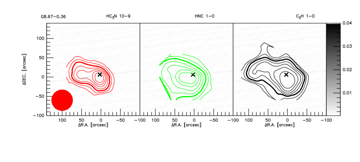
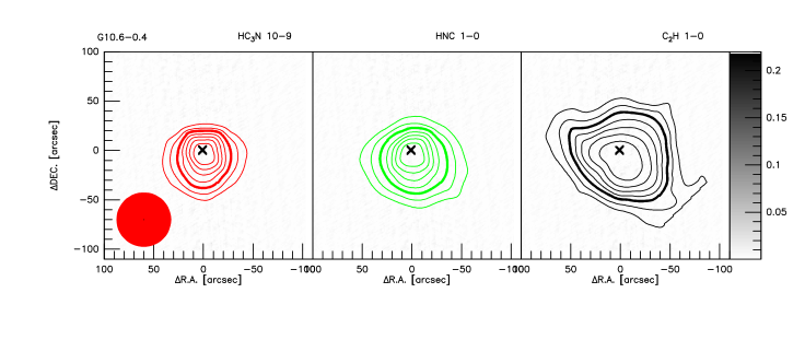
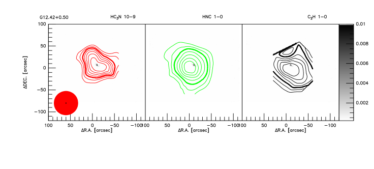
Figure 2: Contour maps of HC₃N 10-9 (left pannel), HNC 1-0 (middle pannel) and C₂H 1-0 (F = 3/2, 2 $\rightarrow$ 1/2, 1) (right pannel) integrated intensity superimposed on its 8.4 or 4.8 GHz continuum map in gray scale. The contour levels are 30%, 40%, 50%, 60%, 70%, 80% and 90% of the map peak, reported in Table 3 (see col. [3] for HC₃N, col. [7] for HNC, and col. [11] for C₂H). The heavy lines represent 50% of the map peak. The FWHM beam size for molecular lines (red big circle) and continuum emission (black small ellipse) observations are shown at the lower left of left map. The water maser is at (0, 0). Crosses are used to mark position of HII region in case that the HII regions are too small to be recognized in the figure. The gray scale range indicated in the wedge is in Jy/beam. (A color version of this figure is available in the online journal.)

Figure 1 shows spectra of HC₃N 10-9, HNC 1-0 and C₂H 1-0 (J = 3/2 $\rightarrow$ 1/2, F = 2 $\rightarrow$ 1) in the observing center for four sources. The line profiles of HC₃N and C₂H could be well fitted with a single Gaussian. The line profiles of HNC could be fitted with a single Gaussian in about half sources. Blue asymmetric structure, named ‘blue profiles’, a combination of a double peak with a brighter blue peak or a skewed single blue peak in optically thick lines (Mardones et al. 1997), has been found in HNC lines in five sources: Cep A, W33cont, W75OH, G121.30+0.66 and W44. Three of these sources have been identified as infalling candidates by Sun et al. (2009) except for W33cont and G121.30+0.66. ‘Red profiles’ are found in source G14.33-0.64, G35.20-0.74, S87 and ON2S. The origin of ‘red profile’ remains unclear, which might be caused by outward motion or rotation. Figure 2 - 10 show contour maps of HC₃N 10-9, HNC 1-0 and C₂H 1-0 (J = 3/2 $\rightarrow$ 1/2, F = 2 $\rightarrow$ 1) imposed on continuum images in gray-scale for 27 clumps. The contours are between 30% and 90% of the peak, in steps of 20% of the peak intensity. The heavy lines in contour maps indicate the half-peak contours. The clumps show various morphologies. Most of them have single peaks, similar to previous CS and HCN observations (Shirley et al. 2005; Wu et al. 2010). The peak antenna temperature (T${}_{A}^{*}$), integrated line intensity ($\int$T${}_{A}^{*}$d$\nu$), LSR velocity, and full-width half-maximum (FWHM) linewidth of HC₃N 10-9, HNC 1-0 and C₂H 1-0 (J = 3/2 $\rightarrow$ 1/2, F = 2 $\rightarrow$ 1) at the central (0, 0) position of the massive dense cores are present in Table 3. All the results are obtained by Gaussian fitting. It should be noted that a single-gaussian fit is insufficient for the optical thick molecular lines of HNC in some sources. Sources that can not be fitted well with a single gaussian are marked with ‘$*$’ in Table 3. HC₃N 10-9 maps of DR21S and S140 have also been observed by Chung et al. (1991) with Nobeyama 45m telescope. Despite the different beam sizes of the Nobeyama 45m and PMO 14m telescope, the morphology and size from two observations are quite consistent. C₂H 2-1 emission of DR21S have been observed by Tucker & Kutner (1978) with NRAO 11m telescope, while C₂H 2-1 and HC₃N 10-9 maps of Cep A have been obtained by Bergin et al. (1996, 1997) with 14m FACRO telescope. The morphology and size from these observations are also consistent with our observations.

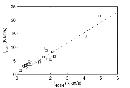
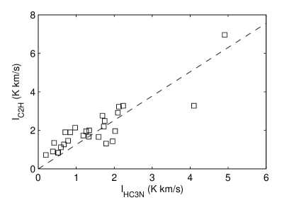
Figure 11: Left: Plot of integrated intensity of HNC averaged over the entire regions versus those of HC₃N. Right: same for C₂H vs. HC₃N. The dashed lines represent the least-square fitting results, with slopes of 3.8 and 1.3.

Figure 11 shows comparison of integrated intensities averaged over the entire regions for three species. A tight correlation between HC₃N and HNC (r=0.92) was found. The result given by least-squares fitting is:

I(HNC) = (3.8 $\pm$ 0.4) $\times$ I(HC₃N).

A very high correlation coefficiency (r=0.88) was also found for average integrated intensities of C₂H and HC₃N (Figure 11). The result given by least-squares fitting is:

I(C₂H) = (1.3 $\pm$ 0.2) $\times$ I(HC₃N).

The tight correlation of intensities between HC₃N, HNC and C₂H imply correlation of the abundance of three species in the early evolutionary stage of massive star-formation.

The size of clouds is characterized using beam deconvolved angular diameter and linear radius of a circle with the same area as the half peak intensity:

$$\theta_{transition}=2(\frac{A_{1/2}}{\pi}-\frac{\theta_{beam}^{2}}{4})^{1/2},$$ (1)

$$R_{transition}=D(\frac{A_{1/2}}{\pi}-\frac{\theta_{beam}^{2}}{4})^{1/2},$$ (2)

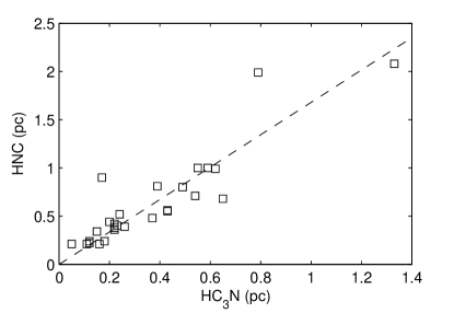
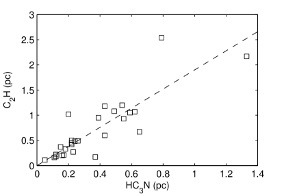
Figure 12: Plot of FWHM size of HNC versus HC₃N (left) and C₂H versus HC₃N (right), and the dashed line represents the least-squares fit result to C₂H vs. HC₃N.

where $A_{1/2}$ is the area within the contour of half peak intensity, $\theta_{beam}$ is the FWHM beam size, and $D$ is the distance of the source. The centroid of velocity-integrated intensity maps, the linear FWHM size and angular FWHM size of clouds for three species are tabulated in Table 4. The radius of HC₃N ranges from 0.05 to 1.33 pc, with a median value of 0.24 pc. Nearly half of cloud sizes derived from HC₃N are smaller than the telescope beam size. The radius of HNC ranges from 0.21 to 2.08 pc, with a median value of 0.44 pc. The FWHM sizes of HNC are well above the beam size. The radius of C₂H clouds ranges from 0.11 to 2.17 pc, with a median value of 0.49 pc. Nearly all the FWHM sizes of C₂H are well above the beam size. Figure 12 shows comparison of FWHM size of three species. Tight correlation was found between FWHM sizes of HNC and HC₃N (r=0.93), as well as between the sizes of C₂H and HC₃N (r=0.85). Results given by least-squares fitting are:

R(HNC) = (1.68 $\pm$ 0.17) $\times$ R(HC₃N),

R(C₂H) = (1.90 $\pm$ 0.18) $\times$ R(HC₃N).

The FWHM sizes shrink as excitation requirements increase, indicating that the clumps are centrally condensed, with either a smooth decrease in density with increasing radius, or an increased fraction of the volume filled by dense “raisins” (Mueller et al. 2002; Wu et al. 2010).

The FWHM linewidths of HC₃N, HNC and C₂H at (0, 0) range from 1.82 to 9.84 km s^-1, 2.07 to 9.96 km s^-1, and 1.07 to 8.68 km s^-1, with median values of 3.18, 4.07 and 3.75 km s^-1, respectively. The largest value of linewidths, 9.96 km s^-1, comes from HNC observation of W51M, while the smallest value, 1.07 km s^-1, comes from C₂H observations of AFGL 490. The linewidths of HNC lines are about 1.2 times larger than those of HC₃N, which should be caused by large optical depth of HNC. The linewidth of HC₃N is larger than that of C₂H or HNC in sources such as G8.67-0.36, G10.6-0.4 and W51M, indicating more violent turbulence in HC₃N emission region than the outward.

3.2 Radio Continuum Emission

In Table 5, we list the peak intensity $S_{p}$ in column (2), flux density $S_{\nu}$ in column (3), the deconvolved size in column (4), position angle in column (5), linear size in column (6), and classification of HII regions in column (7). All the parameters are obtained by fitting one single Gaussian component to the strongest emission peak with AIPS task IMFIT, and the linear size of HII region is calculated using the fitting results of major axis. No prominent continuum emission was detected in G14.33-0.64 ($\sigma\sim$ 0.04 mJy), G59.78+0.06 ($\sigma\sim$ 0.008 mJy) and W75OH ($\sigma\sim$ 0.4 mJy), suggesting that these sources are in early evolutionary phase.

Based on the 2 cm size measurements and densities, stellar ionized regions regions are usually classified as hyper-compact (HCHII) ($\leq$ 0.01 pc), ultra-compact (UCHII) ($\leq$0.1 pc), compact (CHII) ($\leq$0.5 pc) and extended HII regions ($>$0.5 pc or clearly associated with a classical HII regions) (Wood & Churchwell 1989; Kurtz 2000, 2002; Churchwell 2002), which probably represents an evolutionary sequence. It should be noted that the morphology of HII regions is strongly dependent upon the UV-coverage (e.g., long baselines are not sensitive to the extended emission), which makes the classification of HII regions ambiguous. Previous classification is always adopted if available. Most of our sample are classified as UCHII regions, and three sources (S231, S235 and S76E) are classified as extended HII regions.

3.3 Individual Targets

Comparison with previous CS, HCN and 350 $\mu$m dust continuum emission (Mueller et al. 2002; Shirley et al. 2003; Wu et al. 2010) indicates that molecular lines observed here exhibit similar morphologies to CS and HCN for most sources. The molecular emission morphology has a very centrally condensed structure for about half of the sample, with emission peak near to the HII region and the maxima of dust continuum emission. Such a simple structure suggests simple density gradient increasing from the edge of the dense core to the center. Sources with distinctive distributions are discussed below.

W42: The radio continuum map consists of a UCHII and a CHII region. All the molecular line emissions except C₂H peak towards the UCHII region (Shirley et al. 2003; Wu et al. 2010). Both the HNC and C₂H exhibit a single core elongating from southeast to northwest in velocity-integrated intensity maps, while the HC₃N emission is seen to avoid the CHII region. The different spatial distribution of three species around HII regions can be explained by the destruction of HC₃N by UV photons.

W44: The radio continuum map consists of a UCHII region and a supernova remnant. Molecular line emissions peak toward the UCHII region. HNC, C₂H, HCN and CS maps show weak tails toward supernova remnant (Wu et al. 2010).

S76E: An extended HII region is shown in VLA map of S76E. There is a single core in spectral line maps. The molecular line emissions have an offset from peak of the radio continuum emission, which might be caused by relative motion between young stellar objects and molecular clouds. It is also possible that the HII region is not associated with molecular cloud.

G35.20-0.74: Molecular line emissions exhibit similar centrally condensed structure. HC₃N and HNC emissions peak toward CHII region, while C₂H and CS emissions peak to the southeast of CHII region (Shirley et al. 2003; Wu et al. 2010).

W51M: High-resolution centimeter observations reveal several compact continuum components in W51M (e.g., Gaume et al. 1993; Shi et al. 2010). HNC, high J transitions of CS and HCN and dust emission reveal two cores, with the southeast core associated with water masers (Shirley et al. 2003; Wu et al. 2010; Mueller et al. 2002). HC₃N, C₂H and CS emissions peak towards the southeast core, while HNC and HCN peak toward the northwest core. The HC₃N linewidth is widest among all our sample, indicating rather violent turbulence in this source.

G59.78+0.06: No radio continuum emission was detected in this source. Both HC₃N and C₂H emissions are relatively weak in G59.78+0.06. HNC shows similar morphology to HCN and CS emission (Wu et al. 2010), with a single peak away from water masers.

S87: VLA maps of S87 HII region reveal a radio continuum source consisting of a compact core and a fan-shaped tail extending to the southeast (Bally & Predmore 1983; Barsony 1989). There are single core elongated from northeast to southwest in spectral line maps. The peak molecular line emissions obviously offset from both the maxima of radio continuum emission and dust continuum emission (Mueller et al. 2002).

ON2S: The map consists of two molecular clouds. The northern molecular cloud (ON2N) contains the G75.78+0.34 UCHII region excited by an early B star, and the southern cloud (ON2S) contains the G75.77+0.35 HII region excited by an O star (e.g., Matthews & Spoelstra 1983; Dent et al. 1988). Molecular line emissions show similar morphology, with emission peaks slightly offset from UCHII region and the maxima of dust continuum emission (Mueller et al. 2002). It should be noted that the peculiar morphology of C₂H map is mainly caused by the low signal-to-noise ratio (SNR).

DR 21S: The DR 21S massive star-forming region contains two cometary HII regions, aligned nearly perpendicular to each other on the sky. The molecular line emissions peak to the south of HII regions. HC₃N has the most compact emission morphology, while the C₂H has the most extended emission.

W75OH: We did not detect prominent radio continuum emission associated with this source. HC₃N, HNC, CS and HCN emissions show similar morphology, with filaments structure consisting of two cores extending from south to north in spectral line maps (Shirley et al. 2003; Wu et al. 2010). C₂H emission differs significantly from other species, with integrated intensities varying slowly with position, which agrees well with observations of Tucker & Kutner (1978). They attributed it to that C₂H emission is produced almost entirely in the extended molecular clouds containing the rich molecular cores, with little or no emission arising from the dense cores themselves.

W3(OH): Molecular line emissions show similar morphology. Obvious offset between HC₃N emission peak emission and HII regions was found, while other molecular line emissions peak near to HII regions.

S231: The high resolution VLA observation seems to resolve the extended emission, so we adopt it as an extended HII region, following the classification of Israel & Felli (1978). There are single cores in spectral line maps, with emission peak near to HII region and maxima of dust continuum emission (Mueller et al. 2002).

S235: This is an extended HII region. The spectral line maps offset significantly from peak radio continuum emission, which might be caused by the relative motion between young stellar embedded in HII regions and their molecular clouds. The relative motions have been proposed while inspecting the velocity difference between HII regions and molecular clouds, which are found to range from 0.5 to 10 km s^-1 (Zuckerman 1973; Churchwell et al. 2010). The radio recombination line (RRL) of S235 is observed to be -23.07 km s^-1 (Quireza et al. 2006), thus the radial velocity difference between HII region and HC₃N cloud is 6.28 km s^-1, implying possibility of relative motion. Separation between HC₃N centroid and peak emission of HII regions is 28″. At the assumed distances of 1.6 kpc, the separation correspond to 0.22 pc. Adopting a proper motion velocity of 1 km s^-1, we could obtain a timescale of 2$\times$10⁵ yr, which is consistent with the evolution timescale of UCHII regions (e.g., Mellema et al. 2006). The molecular line emissions peak near to the maxima of dust continuum emission (Mueller et al. 2002).

S255: There are single cores elongated from northwest to southeast in spectral line maps. The HC₃N and HNC emissions peak toward UCHII region, which is 60″ north of water masers. CS and HCN peak close to water masers, while the maxima of C₂H emission lies in between water masers and UCHII region.

S140: There are single cores elongated from northeast to southwest in molecular line maps. HC₃N and HNC emission peak toward radio continuum emission and water masers, but slightly offset from the maxima of dust continuum emission (Wu et al. 2010). C₂H emission peak offset from HII region and water masers by about half beam.

Previous observations suggest that HC₃N is easily destroyed by UV photons (e.g., Rodriguez-Franco et al. 1998; Gwenlan et al. 2000). Though angular resolution seems too coarse to investigate this issue, observations present here could give us some hints, e.g., separations larger than $\theta_{mb}/2$ are found between the maxima of radio continuum emission and HC₃N emission in S87 and S235. Different spatial distribution between HC₃N and other molecular lines in W42 also support that point.

4 DISCUSSIONS

4.1 Central Depletion of C₂H

We can use the hyperfine components to obtain the C₂H optical depth. In Figure 13 we show an example of a C₂H spectra for Cep A. The spectra are averaged over the entire emitting region. As is shown in the figure, C₂H 1-0 has six hyperfine components (J = 3/2 $\rightarrow$ 1/2, F = 1 $\rightarrow$ 1; J = 3/2 $\rightarrow$ 1/2, F = 2 $\rightarrow$ 1; J = 3/2 $\rightarrow$ 1/2, F = 1 $\rightarrow$ 0; J = 1/2 $\rightarrow$ 1/2, F = 1 $\rightarrow$ 1; J = 1/2 $\rightarrow$ 1/2, F = 0 $\rightarrow$ 1; J = 1/2 $\rightarrow$ 1/2, F = 1 $\rightarrow$ 0). If the C₂H 1-0 line is optically thin and the hyperfine levels are populated according to LTE, the line ratios between the six hyperfine components approximate 1:10:5:5:2:1. The intrinsic relative intensities of the hyperfine components are taken from Tucker et al. (1974). We estimated the optical depth of C₂H 1-0 (J = 3/2 $\rightarrow$ 1/2, F = 2 $\rightarrow$ 1) by fitting the lines using METHOD HFS of the CLASS program, which is part of the GILDAS package. This method assumes that all the hyperfine components have the same excitation temperature and broadening with fixed separation according to the laboratory value. Note that CLASS HFS METHOD could only provide correct fitting results for optical depth larger than 0.1.

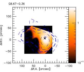
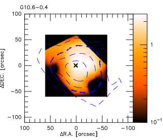
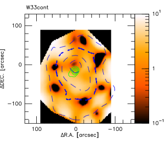
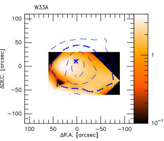
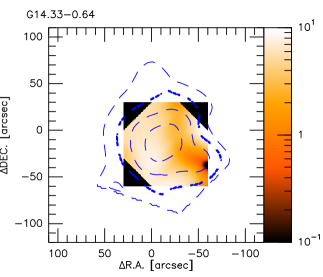
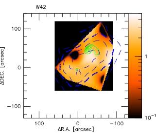
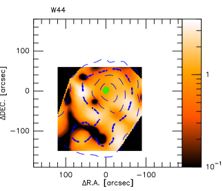
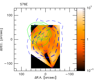
Figure 14: Contour maps C₂H 1-0 (J = 3/2$\rightarrow$1/2, F = 2$\rightarrow$1) (dashed line) integrated intensity and radio continuum emission (solid line) superimposed on the optical depth of C₂H 1-0 (J = 3/2$\rightarrow$1/2, F = 2$\rightarrow$1) in gray scale. Dashed lines represent contour levels of 30%, 50%, 70% and 90% of the peak intensity of C₂H emission, reported in Table 3. Solid lines represent contour levels of 30%, 50%, 70% and 90% of the peak intensity of radio continuum emission, reported in Table 5. Crosses are used to mark position of HII regions in case that the HII regions are too small to be recognized in the figure. (A color version of this figure is available in the online journal.)

In Table 6, we list optical depth of spectral line averaging over the whole emitting region $\tau_{aver}$ in column (2), optical depth of spectral line at (0, 0) $\tau_{0,0}$ in column (3), maximum optical depth $\tau_{max}$ in column (4), and offset of spectral line with $\tau_{max}$ in column (5). Note that results present here are optical depth of the main hyperfine line. $\tau_{aver}$ ranges from 0.10 to 5.37, with a median value of 1.16. $\tau_{0,0}$ is smaller than $\tau_{aver}$ for source W33cont, ON1, DR21S, S140 and NGC2264. For most sources the offset of $\tau_{max}$ is different from C₂H centroid. Such trend is also reflected in the opacity maps. Figure 14 - 16 show velocity integrated contour maps of C₂H 1-0 (F = 3/2, 2 $\rightarrow$ 1/2, 1) superimposed on opacity maps of C₂H 1-0 (J = 3/2 $\rightarrow$ 1/2, F = 2 $\rightarrow$ 1) in gray-scale. The optical depth has obvious dip toward the emission peak of C₂H in eight sources, such as DR21S, Cep A, W51M, ON1 and NGC2264. Since optical depth is a direct measurement of column density, thus the C₂H column density should decrease toward the centroid for these sources, which is well consistent with chemical model of C₂H (Beuther et al. 2008; Padovani et al. 2009; Walsh et al. 2010). However, some sources donot show signature of C₂H depletion toward hot cores or HII regions, such as G14.33-0.64, G8.67-0.36, W33A. Limited by low resolution (FWHP$\sim$55″) and high rms noise level ($\sim$0.2 K with velocity resolution of $\sim$0.21 km s^-1) of our observations, it is hard to tell whether this is intrinsic to these sources or not.

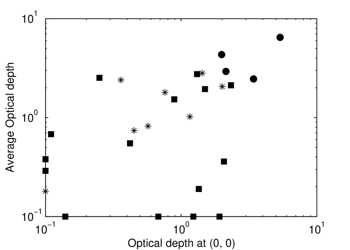
Figure 17: Plot of optical depth for C₂H 1-0 main line at (0, 0) versus optical depth of C₂H 1-0 main line averaging over the whole emitting regions. Sources not associated with a detectable HII regions and sources associated with HCHII regions are plotted as circles. Sources associated with UCHII regions are plotted as squares, while sources associated with CHII or extended HII regions are shown in stars. (A color version of this figure is available in the online journal.)

Figure 17 shows $\tau_{(0,0)}$ versus $\tau_{aver}$ for observing sources. Sources in which no radio continuum emission has been detected and those associated with HCHII regions are plotted as circles. Sources associated with UCHII region are shown in squares, while sources associated with CHII or HII region are plotted as star. One could see clearly from the figure that those “young” molecular clouds that associate with HCHII or not associated with detectable HII regions have larger optical depth than “elder” molecular clouds that associated with UCHII, CHII or extended HII regions. The optical depth of our sample is much smaller than two prestellar cores observed by Padovani et al. (2009), in which the total optical depth ($\tau_{total}=\frac{\tau_{main}}{0.4167}$) ranges from 13.5 to 29.4. These results suggest that C₂H abundance decreases as molecular clouds evolve from hot cores to extended HII regions. Thus C₂H might be used as “chemical clock” for molecular clouds.

4.2 Large-Scale Kinematic Structure of Molecular Clouds

4.2.1 Velocity Gradient

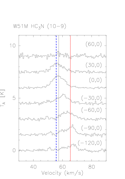
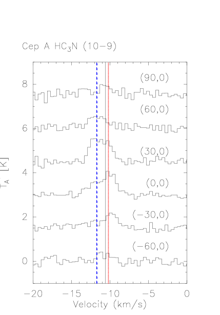
Figure 18: Left: Spectra of HC₃N (10-9) at the offset position of $\triangle Dec=0$ for W51M. The blue dashed line mark centroid velocity for spectra line at (30, 0), while the solid line marks centroid velocity of spectral line at (0, 0), and the red dotted line marks centroid velocity for spectra line at (-120, 0). Right: Spectra of HC₃N (10-9) at the offset position of $\triangle Dec=0$ for Cep A. The blue dashed line mark centroid velocity of spectra line at (60, 0), while the solid line marks centroid veloicty of spectra line at (0, 0), and the red dotted line marks centroid velocity of spectra line at (-30, 0). Centroid velocities are derived from Gaussian fit. (A color version of this figure is available on line.)

Molecular line observations of different density tracers provide good opportunity to analyze the kinematic structure of GMC. Figure 18 shows spectra of HC₃N (10-9) at the offset position of $\triangle Dec=0$ for W51M and Cep A. The dashed lines, solid lines and dotted lines are used to mark centroid velocities for spectral lines at different offset in right ascension. The centroid velocity shifts are about 9.3 km s^-1 and 1.5 km s^-1 for W51M and Cep A, respectively, implying presence of large-scale rotation in molecular clouds (Mardones et al. 1997). We obtain velocity gradients with the gradient calculation method formulated in Goodman et al. (1993) by fitting the function:

$$v_{LSR}=v_{0}+a\vartriangle\alpha+b\vartriangle\beta,$$ (3)

where $v_{LSR}$ represents an intensity-weighted average velocity along the line of sight through the cloud, $v_{0}$ is the systematic velocity of the cloud, with respect to the local standard of rest, $\vartriangle\alpha$ and $\vartriangle\beta$ represent offsets in right ascension and declination in radians, and a and b are the projections of the gradient per radian on the $\alpha$ and $\beta$ axis. The magnitude of the velocity gradient, in a cloud at distance $D$, is

$$Grad=\frac{(a^{2}+b^{2})^{1/2}}{D},$$ (4)

and its direction (the direction of increasing velocity, measured east of north) is given by

$$\theta=tan^{-1}\frac{a}{b}.$$ (5)

Only points with integrated intensities above 3$\sigma$ levels are used in the calculation. As is stated in Goodman et al. (1993), maps with fewer than nine detections could not be fitted reliably, so we excluded results of any fits to fewer than nine points. Result of gradient fitting for three species, including magnitude of velocity gradient ($Grad$), direction of velocity gradient ($\theta$), ratio of rotation kinetic energy to gravitation energy ($\beta$), and specific angular momentum ($J/M$) are tabulated in Table 7. Significant gradients ($Grad\geq 3\sigma_{Grad}$) were detected in 17, 26 and 18 sources for HC₃N, HNC and C₂H, respectively. Note that only significant gradient ($Grad\geq 3\sigma_{Grad}$) are used in the following discussions. Fewer detections in HC₃N are mainly caused by small size of HC₃N maps, some of which donot have enough data points. This is also the case for HNC map of ON2S and ON2N. The high detection rate with HNC ($\sim$100%) suggests that rotation should be quite common and present in nearly all molecular clouds.

The derived gradients of HC₃N range from 0.24 to 6.03 km s^-1 pc^-1, with a median value of 1.43 km s^-1 pc^-1. The detected gradients of HNC range from 0.13 to 3.58 km s^-1 pc^-1, with a median value of 0.76 km s^-1 pc^-1. The detected gradients of C₂H range from 0.25 to 3.70 km s^-1 pc^-1, with a median value of 0.85 km s^-1 pc^-1. Velocity gradients in some of our targets have already been detected in previous studies, such as S235, S140, AFGL490 (Higuchi et al. 2010), G10.6-0.4 (e.g., Keto et al. 1987; Liu et al. 2010) and W75OH (Schneider et al. 2010). The velocity gradients derived using Nobeyama 45m observations of H¹³CO⁺ range from 0.5 km s^-1 pc^-1 to 4.3 km s^-1 pc^-1 (Higuchi et al. 2010), which are in agreement with results present here.

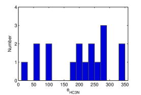
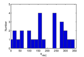
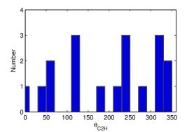
Figure 19: Distribution of gradient direction ($Grad\geq 3\sigma_{Grad}$) for HC₃N, HNC and C₂H.

Figure 19 shows distribution of direction of detected gradients. The gradient directions show no signature of alignment with the overall direction of Galactic rotation, which is consistent with observations of early-type stars and field Ap stars, in which random orientation of rotational axes are observed (eg., Fleck & Clark 1981; Imara & Blitz 2011). The result supports the idea that the initial cloud angular momentum is unlikely to come from Galactic rotation.

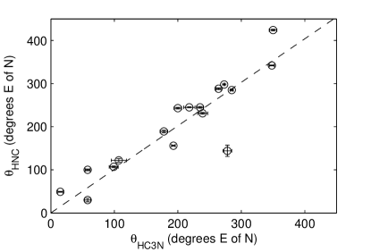
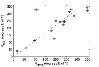
Figure 20: Comparison of gradient direction for HC₃N and HNC (left), HC₃N and C₂H (right). The dashed lines indicate the best-fit relation, with slope of 1.01$\pm$0.12 and 1.10$\pm$0.23, respectively.

Figure 20 shows comparison of gradient direction between HNC and HC₃N, as well as C₂H and HC₃N. Results of least-squares fitting and calculated correlation coefficients ($r$) are as follows:

$\theta_{HNC}$ = (1.01$\pm$0.12)$\times\theta_{HC_{3}N}$, $r$ = 0.91,

$\theta_{C_{2}H}$ = (1.10$\pm$0.23)$\times\theta_{HC_{3}N}$, $r$ = 0.80.

Since HC₃N traces inner denser region, results above indicate than the gradients orientation are preserved over a range of density and these tracers are indeed mapping out a real physical entity. This is consistent with results of Goodman et al. (1993).

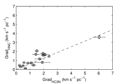
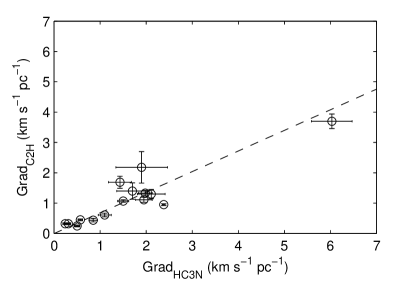
Figure 21: Comparison of gradient magnitude for HC₃N and HNC (left), HC₃N and C₂H (right). The dashed lines indicate the best-fit relation, with slope of 0.63$\pm$0.08 and 0.68$\pm$0.10.

Figure 21 shows comparison of gradient magnitude of HNC, HC₃N and C₂H. Tight correlation between three species were found and the least-squares fitting results and correlation coefficients are as follows:

$Grad_{HNC}$ = (0.63$\pm$0.08)$\times Grad_{HC_{3}N}$, $r$ = 0.89,

$Grad_{C_{2}H}$ = (0.68$\pm$0.10)$\times Grad_{HC_{3}N}$, $r$ = 0.91.

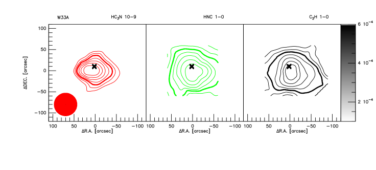
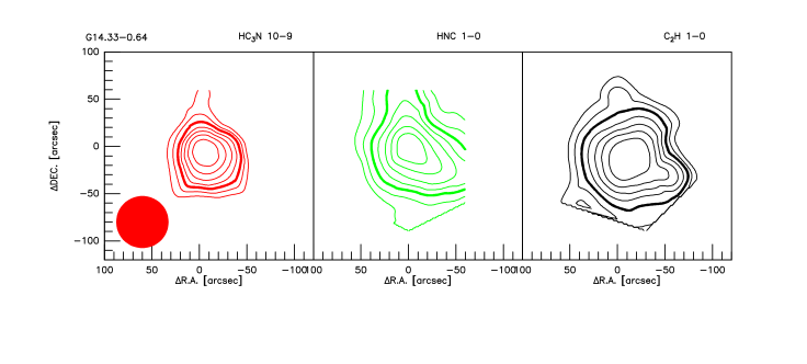
Figure 3: Contour maps of HC₃N 10-9 (left pannel), HNC 1-0 (middle pannel) and C₂H 1-0 (F = 3/2, 2 $\rightarrow$ 1/2, 1) (right pannel) integrated intensity superimposed on its 8.4 or 4.8 GHz continuum map in gray scale. (A color version of this figure is available in the online journal.)

It is evident that the magnitude of gradient increase toward the inner region, $\omega\propto\frac{1}{R}$, thus most of those molecular clouds should experience differential rotation, rather than rigid-body rotation ($\omega$ constant). In addition, the rotation velocity $v$ remains constant. These results are opposite of what is expected based on angular momentum conservation. It seems to be well consistent with MHD simulation of Mellon & Li (2009). They studied the effects of ambipolar diffusion on magnetic braking and disk formation and evolution during the main accretion phase of star formation. Their results show that rotation velocity $v$ is nearly constant in the region $6\times 10^{15}$ cm $\leq r\leq 1\times 10^{17}$ cm (see Figure 3 of Mellon & Li 2009) because of angular momentum loss caused by magnetic braking. The specific angular momentum was computed in Section 4.2.3 to better illustrate this point.

4.2.2 Ratio of Rotation Kinetic Energy to Gravitational Energy

The parameter $\beta$, which is defined as the ratio of rotational energy to the gravitational potential energy, is always used to quantify the dynamical role of rotation in a cloud. It could be written as (Goodman et al. 1993):

$$\beta=\frac{(1/2)I\omega^{2}}{qGM^{2}/R}=\frac{1}{2}\frac{p}{q}\frac{\omega^{2}R^{3}}{GM},$$ (6)

where I is the moment of inertia, which is given by $I=pMR^{2}$ for the particular shape and density distribution of the cloud, and $qGM^{2}/R$ represents the gravitational potential energy of mass $M$ within radius $R$. For a uniform density sphere, $q=\frac{3}{5}$ and $p=\frac{2}{5}$, thus $p/q=\frac{2}{3}$. For a sphere with an density profile of $r^{-2}$, $p/q=0.22$, which reduces $\beta$ for fixed $M$, $\omega$ and $R$, by a factor of 3 comparing with the uniform density case.

For a sphere with constant density $\rho_{0}$, it could be written as (Goodman et al. 1993):

$$\beta=\frac{1}{4\pi G\rho_{0}}\omega^{2}=\frac{1}{4\pi G\rho_{0}}\frac{Grad^{2}}{sin^{2}i},$$ (7)

where sin i is assumed to be 1 in our calculation. The density of clouds are calculated using virial mass (e.g., Shirley et al. 2005). The virial mass of the clouds with power-law density distribution is given by

$$M_{Vir}(R)=\frac{5R\triangle v^{2}}{8a_{1}a_{2}Gln2}=209\frac{(R/1pc)(\triangle v/1kms^{-1})}{a_{1}a_{2}}M_{\odot};$$ (8)

$$a_{1}=\frac{1-p/3}{1-2p/5},p<2.5,$$ (9)

where $a_{1}$ is the correction for power-law density distribution and $a_{2}$ is the correction for a nonspherical shape (Bertoldi & McKee 1992). For aspect ratios less than 2, $a_{2}\sim$ 1 and can be ignored for our sample. An average $p$ value of 1.77 from Mueller et al. (200) is adopted to calculate $a_{1}$ for all clouds. The FWHM linewidth of clouds, $\triangle v$, are determined from a Gaussian fitting to the average spectra over regions of half power contour.

The calculated $\beta$ for three species are listed in Table 7. $\beta_{HC_{3}N}$ range from 0.0006 to 0.028, with a median value of 0.011, $\beta_{HNC}$ range from 0.0001 to 0.067, with a median value of 0.018, and $\beta_{C_{2}H}$ range from 0.0012 to 0.032, with a median value of 0.012. Results presented here seem to be consistent with previous observations of NH₃, in which molecular clouds were observed to have $\sim$2% rotational energy against gravitational energy (Goodman et al. 1993). $\beta_{C_{2}H}$ seem to be smaller than $\beta_{HNC}$, implies that C₂H should arise from more extended and diffuse components, which is consistent with observations of Tucker & Kutner (1978). It is noted that Goodman et al. (1993) have pointed out that gradients determined using low-density tracers can be contaminated by gas at the size scale most populated by that tracer, and thus can give inappropriate estimate of $\beta$, a result also suggested by the analysis in Arquilla & Goldsmith (1986).

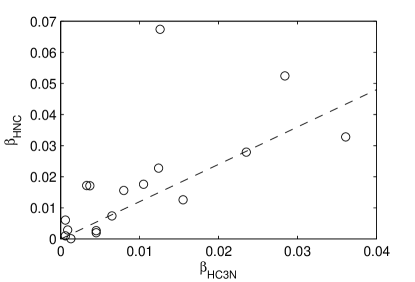
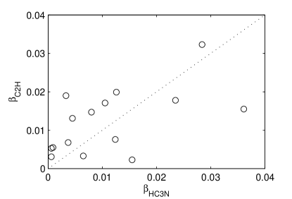
Figure 22: Comparison of ratio of rotational energy to gravitational energy $\beta$ for HC₃N and HNC (left), HC₃N and C₂H (right). The dashed line in the left figure indicate the best-fit relation, with slopes of 1.48$\pm$0.52. The slope of the dotted line in the right figure is 1.

Goodman et al. (1993) found that $\beta$ is roughly independent of size in their analysis of NH₃ observations, but they caution that it is necessary to measure $\beta$ using several density tracers in individual cores in order to avoid density selection effects. In Figure 22 we show comparison of $\beta$ among three molecular lines. Correlation coefficient between $\beta_{HNC}$ and $\beta_{HC_{3}N}$ is 0.62. We also carried out least-squares fitting to data of HNC and HC₃N:

$\beta_{HNC}$ = (1.48$\pm$0.52)$\times$ $\beta_{HC_{3}N}$.

Correlation coefficient between $\beta_{C_{2}H}$ and $\beta_{HC_{3}N}$ is only 0.52, so we did not carry out least-square fitting. A dotted line with a slope of 1 is plotted for reference (Figure 22 (right)). We can see from the figure that $\beta_{C_{2}H}$ is larger than $\beta_{HC_{3}N}$ for 10 sources (67%). Thus we conclude that the ratio of rotational kinetic energy to gravitational energy does depend on size and decreases toward the center. These results indicate that the dynamical importance of rotation decreases toward the central core.

4.2.3 Specific Angular Momentum

The specific angular momentum $J/M$ is calculated using $\frac{J}{M}=p\omega$R², $p=\frac{2}{5}$ for a uniform density sphere. The decrease of $J/m$ from large to small scales has been found in protostellar sources (Goodman et al. 1993; Ohashi et al. 1997; Liu et al. 2010). However, most of these studies are derived using single tracers and careful examination of a large sample of clouds are required to characterize the evolution of $J/M$ within single cores.

The calculated $J/M$ for three species are listed in Table 7. $J/M$ of HC₃N range from 0.0072 to 1.68 km s^-1 pc^-1, with a median value of 0.16 km s^-1 pc^-1, corresponding to 5.1$\times$ 10²² cm${}^{2}~{}$s^-1; $J/M$ of HNC range from 0.0024 to 2.50 km s^-1 pc^-1, with a median value of 0.28 km s^-1 pc^-1, corresponding to 8.5$\times$ 10²² cm² s^-1; and $J/M$ of C₂H range from 0.014 to 1.8 km s^-1 pc^-1, with a median value of 0.24 km s^-1 pc^-1, corresponding to 7.5$\times$ 10²² cm² s^-1. Results presented here are an order of magnitude larger than previous results (Goodman et al. 1993; Caselli et al. 2002). Since most of sources in Goodman et al. (1993) are low-mass dense cores, massive star-forming regions seem to have larger specific angular momentum. Seven objects of our sample, including G121.3+0.66, W3(OH), AFGL 490, S231, NGC 2264, W75OH and S140, have been observed in N₂H⁺ 1-0 transition by Pirogov et al. (2003). Velocity gradients, ratio of rotation to gravitational energy and specific angular momentum of these objects were derived with N₂H⁺ observations. Their results are not exactly the same as results present here since N₂H⁺ and HC₃N, HNC and C₂H trace different gas, and the beam size of their observations are also different from our observations. However, they all have same trends.

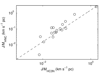
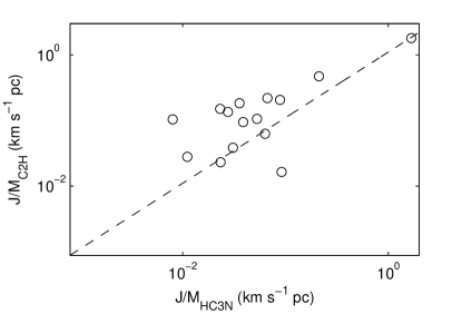
Figure 23: Comparison of specific angular momentum $J/M$ for HC₃N and HNC (left), HC₃N and C₂H (right). The dashed lines indicate the best-fit relation, with slopes of 1.54$\pm$0.17 and 1.10$\pm$0.13, respectively.

Figure 23 shows comparison of J/M between three species. Correlation coefficient between $J/M$ of HNC and HC₃N is 0.92. Least-Squares fitting result is as follows:

$J/M_{HNC}$ = (1.54$\pm$0.17)$\times$ $J/M_{HC_{3}N}$.

Correlation coefficient between $J/M$ of C₂H and HC₃N is 0.92. Least-Squares fitting result is as follows:

$J/M_{C_{2}H}$ = (1.10$\pm$0.13)$\times$ $J/M_{HC_{3}N}$.

These results imply obvious decline of $J/M$ toward central regions from $\sim$2 pc to $\sim$ 0.1 pc. Thus the angular momentum transfer not only occurs at small scale ($<$ 0.1 pc) (Liu et al. 2010), but also occurs at large scale. Magnetic braking and outflow are thought to be possible mechanism for angular momentum transfer (e.g., Mouschovias & Paleologou 1979; Fleck & Clark 1981; Mestel & Paris 1984; Rosolowsky et al. 2003). Since outflow is unlikely to be responsible to angular momentum transfer in large scale, magnetic braking, in which magnetic field lines anchoring molecular cloud to the ambient interstellar matter provide the tension necessary to slow down rotation, seems to be the most possible explanation for the decrease of specific angular momentum. Results present here allow us to put some constraints on the magnetic field strength. Numerical simulation indicates that whether the evolution of a collapsing core is regulated by the centrifugal forces or by magnetic forces depends on the value of the rotation velocity and magnetic field strength $\omega/B$ (Machida et al. 2005; Girart et al. 2009). If the measured $\omega/B$ is larger than $\frac{\omega_{st}}{B}_{crit}=1.69\times 10^{-7}\times(\frac{c_{s}}{0.19km/s})^{-1}$ year${}^{-1}\mu$ G^-1, where $c_{s}$ is the sound speed and $\omega$ is the angular velocity, the centrifugal forces dominate the dynamics. Otherwise the magnetic forces regulate the dynamics. The median velocity gradient derived using HC₃N is 1.43 km s^-1 pc^-1, corresponding to $1.45\times 10^{-6}$ year^-1. For $c_{s}$=0.19 km s^-1, we found a critical magnetic field strength of 9$\mu$G. Thus, the magnetic field should be larger than several $\mu$G to dominate the dynamics of the collapse.

4.3 Implication for Magnetic Field of Molecular Clouds

Magnetic field is believed to play an important role in the evolution of molecular clouds and star formation. Magnetic fields appear to provide the only viable mechanism for transporting excess angular momentum from collapsing cores, thus allowing continuous accretion, and they may play a significant role in the physics of bipolar outflows and jets that accompany protostar formation (e.g., Falgarone et al. 2008; Girart et al. 2009). The magnetic field of a cloud is probably its most difficult property to obtain. For many years observational studies of magnetic fields in molecular clouds are restricted to probe the line-of-sight component via the Zeeman effect of molecular lines (eg., HI, OH, CN), or the plane of sky component via polarization measurements of the thermal radiation emitted by magnetically aligned aspherical dust grains. All these measurements require observations with both high stability and high signal to noise ratio, and are therefore quite difficult and time consuming (e.g., Bourke & Goodman 2004; Bergin & Tafalla 2007).

The idea that interstellar magnetic fields may be coupled to gas motions was first discussed by Alfv$\acute{e}$n (1943) and Fermi (1949). When the interstellar medium contains a well-coupled magnetic field, disturbances should propagate at the Alfv$\acute{e}$n velocity, $V_{A}=B/(4\pi mn)^{1/2}$, where $B$ represents the mean magnetic field strength, $m$ represents the mean molecular mass (2.33 amu), and $n$ represents the number density. Myers & Goodman (1988) develops a uniformly magnetic sphere model to derive magnetic field strength and number density of the dense cores from the FWHM linewidth. In this model, the supersonic linewidth is attributed to magnetic motions, and the upper limit of the magnetic field could be estimated via comparing the nonthermal contribution of a cloud’s velocity dispersion, $\sigma_{NT}$, to its Alfv$\acute{e}$n velocity. The model cloud is a uniform self-gravitating sphere of mass $M$, radius $R$, number density $n$, temperature $T$, and mean magnetic field strength $B$. It is surrounded by a medium of negligible kinetic and magnetic pressure. It is in virial equilibrium between self-gravity, magnetic energy and its internal random motions,

$$3nkT+\frac{B^{2}}{4\pi}-\frac{3GMmn}{5R}=0,$$ (10)

where $m$ is the mean molecular weight. Equation above could also be written as:

$$\frac{GM}{5R}=\sigma_{T}^{2}+\sigma_{NT}^{2}.$$ (11)

This relation models the virial equilibrium trend reported by Larson (1981). The nonthermal velocity dispersion is taken to be the difference between the observed velocity dispersion and the thermal component:

$$\sigma_{NT}^{2}=\sigma_{obs}^{2}-\sigma_{T}^{2}=\frac{\triangle V_{obs}^{2}}{8ln2}-\frac{kT}{\mu_{obs}},$$ (12)

where $\triangle V_{obs}$ is the FWHM linewidth of the observed molecule, $\mu_{obs}$ is the molecule’s mass, and $T$ is the kinetic temperature of the gas. The nonthermal kinetic energy density is assumed to be equal to the magnetic energy density, as given by Spitzer (1978):

$$\sigma_{NT}^{2}=\frac{2}{3}\frac{B^{2}}{8\pi mn}=\frac{v_{A}^{2}}{3}.$$ (13)

Finally, magnetic field strength and number density could be obtained by solving equations above:

$$B=\frac{3\sigma_{NT}}{R}[\frac{5}{G}(\sigma_{T}^{2}+\sigma_{NT}^{2})]^{1/2}.$$ (14)

$$n=\frac{15}{4}\frac{1}{\pi GR^{2}m}(\sigma_{T}^{2}+\sigma_{NT}^{2}).$$ (15)

Zheng & Huang (1996) derived the magnetic field strength of the dense cores in the Orion B molecular cloud from the FWHM linewidth based on the model of a uniformly magnetic sphere. Average magnetic field strength of 110 $\mu$G is obtained, which is agreed closely to those derived from observations of Zeeman splitting of HI and OH. They also obtained an average number density of 8$\times 10^{4}$ cm^-3, which agreed with those derived using observations of NH₃. They suggested that this method could be applicable to the cores of R$>$0.2 pc.

Optically thick lines should be avoided to obtain the true velocity dispersion from the linewidth, thus only HC₃N observations are suitable to derive the magnetic field strength and number density. Rotation could also contribute to the observed linewidth for rotating clouds. For a cloud at a distance of $D$, a 55″ beam would give $\sigma_{rot}=D\times\frac{55}{60\times 60}\times\frac{\pi}{180}\times Grad$. The rotation line broadening is calculated to range from 0.14 to 3.43 km s^-1, with a median value of 0.76 km s^-1. The rotational line broadening and rotational energy should be taken into account for clouds in which velocity gradients are detected. Thus Equation (10), (11) and (12) should be written as:

$$3nkT+\frac{B^{2}}{4\pi}-\frac{3GMmn}{5R}+2\times\frac{\frac{1}{2}I\omega^{2}}{V}=3nkT+\frac{B^{2}}{4\pi}-\frac{3GMmn}{5R}+\frac{2mnR^{2}\omega^{2}}{5}=0,$$ (16)

$$\frac{GM}{5R}-\frac{2R^{2}\omega^{2}}{15}=\sigma_{T}^{2}+\sigma_{Turb}^{2},$$ (17)

$$\sigma_{Turb}^{2}=\sigma_{obs}^{2}-\sigma_{T}^{2}-\sigma_{rot}^{2}=\frac{\triangle V_{obs}^{2}}{8ln2}-\frac{kT}{\mu_{obs}}-\sigma_{rot}^{2},$$ (18)

where $\sigma_{Turb}$ represents turbulent line broadening.

Magnetic field strength and number density could be obtained by solving Equation (16), (17) and (18):

$$B=\frac{3\sigma_{Turb}}{R}[\frac{5}{G}(\sigma_{T}^{2}+\sigma_{Turb}^{2}+\frac{2}{15}R^{2}\omega^{2})]^{1/2}.$$ (19)

$$n=\frac{15}{4}\frac{1}{\pi GR^{2}m}(\sigma_{T}^{2}+\sigma_{Turb}^{2}+\frac{2}{15}R^{2}\omega^{2}).$$ (20)

Single-dish ammonia observations of water maser sources reveal molecular gas temperature of 10-20 K (Codella et al. 1997). Zheng & Huang (1996) found that both the magnetic field strength and number density are insensitive to temperature. For a dense core with R = 0.25 pc, $\delta$ v = 1.5 km s^-1, the difference is only 8% for magnetic field strength derived using 20K and 10K, while the difference is only 5% for number densities derived using 20K and 10K. Thus a temperature of 20 K was adopted here. Gradients derived using HC₃N are adopted if available, otherwise Gradients derived using HNC will be used. Table 8 presents the rotation line broadening $\sigma_{rot}$ in column (2), turbulence broadening $\sigma_{Turb}$ in column (3), derived magnetic field strength in column (4), and number density in column (5). The magnetic field strength ranges from 3 $\mu$G to 88 $\mu$G, with a median value of 13 $\mu$G. Falgarone et al. (2008) carried out CN Zeeman measurements toward 14 star-forming regions and obtained a median value of 560 $\mu$G. It is no wonder that results derived here are much smaller, since it is averaged over the FWHM contours. The major uncertainty comes from the volume filling factor, which makes it difficult to unambiguously determine source radius R. Thus B and n are probably under estimate of actual values. The strongest magnetic field comes from W51M, which has been indicated in previous polarization observations of water maser and thermal dust emission of this region (Lepp$\ddot{a}$nen et al. 1998; Lai et al. 2001). This source would be an excellent candidate for future Zeeman measurements of CN or C₂H. The derived number densities range from 2.4$\times$10⁴ to 1.2$\times$10⁶ cm^-3, with a median value of 1$\times$10⁵ cm^-3, which agrees closely with critical density of HC₃N 10-9 (Chung et al. 1991).

The mass-to-flux ratio $M/\phi_{B}$ is a quantitative measure of whether the molecular cloud is magnetically supercritical (i.e., the magnetic field cannot resist the gravitational collapse) or subcritical (i.e., the magnetic field could resist the gravitational collapse) (e.g., Crutcher et al. 1996, 1999). The critical value of ratio, $M/\phi_{B}=c_{\phi}/\sqrt{G}$, with $c_{\phi}=0.126$ for disks with only thermal support along field lines, was derived by Mouschovias & Spitzer (1976). Tomisaka et al. (1988) found a $c_{\phi}$ of 0.12 from extensive numerical calculations. The mass-to-flux ratio $M/\phi_{B}$, in units of the critical value of $M/\phi_{B}$, is $10^{-20}\times N(H_{2})/|B|$ cm${}^{2}\mu$ G, where $N(H_{2})$ is the average column density and could be written as $(4/3)Rn$. Due to difficulties in magnetic field strength measurements, $M/\phi_{B}$ is still uncertain. Many cores have only lower limits. The uniformly magnetic sphere model appears to provide a reasonable estimate of $M/\phi_{B}$ as it gives the average magnetic field strength and number density. $M/\phi_{B}$ is calculated to be 72 times critical with the median magnetic field strength of 13 $\mu$G, median number density of 1$\times$10⁵ cm^-3 and median radius of 0.24 pc. This means that the molecular clouds are strongly supercritical and magnetic fields alone are insufficient to support clouds against gravity. V$\acute{a}$zquez-Semadeni et al. (2011) have recently found that clouds formed by supercritical inflow streams proceed directly to collapse, while clouds formed by subcritical streams first contract and then re-expand, oscillating on the scale of tens of Myr. Their simulations with initial magnetic field strength of several $\mu$G also show that only supercritical lead to reasonable star forming rates. This result is not altered by the inclusion of ambipolar diffusion. Thus we could see that both magnetic field strength and number density derived using the uniformly magnetic sphere model are not in contradiction with observations and numerical simulations, indicating possible magnetic field origin of turbulence, as is suggested by Zeeman measurements of magnetic field strengths (Crutcher et al. 1999; Falgarone et al. 2008). Turbulence is another important support against gravity besides magnetic field, understanding of the origin of turbulence is critical to our understanding of massive star-formation. More observations are needed to further investigate the relationship between magnetic field and the origin of turbulence.

4.4 Galactic Trends

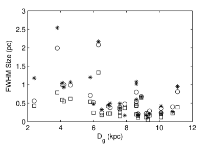
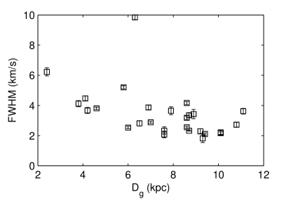
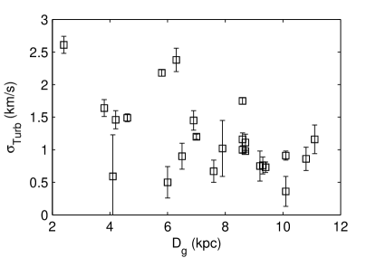
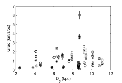
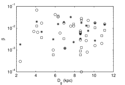
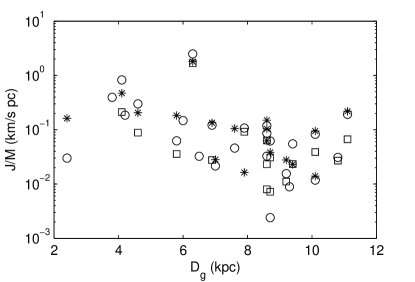
Figure 24: Plot of FWHM sizes, linewidths, $\sigma_{Turb}$, velocity gradients, $\beta$ and specific angular momentum $J/M$ versus galactocentric distance for HC₃N (square), HNC (circle) and C₂H (star).

The FWHM size, linewidth, velocity gradient, $\beta$ and $J/M$ are plotted versus Galactic radius in Figure 24. There is little evidence for any trend in velocity gradient (r=0.13, 0.07 and 0.26 for HC₃N, HNC and C₂H), $\beta$ (r=-0.13, -0.24 and 0.09 for HC₃N, HNC and C₂H). There may be weak anti-correlations of $J/M$ (r=-0.30, -0.26 and -0.29 for HC₃N, HNC and C₂H). Possible anti-correlations are found for FWHM size (r=-0.48, -0.51 and -0.57 for HC₃N, HNC and C₂H), FWHM linewidth of HC₃N (r=-0.50), as well as $\sigma_{Turb}$ (r=-0.53). We just plot FWHM linewidth and $\sigma_{Turb}$ for HC₃N since only HC₃N emission is optically thin among three molecular line emissions, thus only line profile of HC₃N avoids being affected by self-absorption. The large spike in FWHM linewidth near $D_{g}=6.4kpc$ is due to observations of W51M. These results suggest decline of turbulence and dense gas abundance toward outer Galaxy. Our results seem to be inconsistent with observations of CS, in which few trends with galactocentric distance was found (e.g., Zinchenko 1995, 1998; Shirley et al. 2003). Observations of larger samples are needed to support these results.

5 SUMMARY

We conducted mapping observations toward 27 massive star-forming regions associated with water masers with the PMO 14m telescope in the HC₃N 10-9, HNC 1-0 and C₂H 1-0 lines. Maps of HC₃N 10-9, HNC 1-0 and C₂H 1-0 main lines are presented in this paper. The radio continuum emission is searched to characterize the evolutionary stage of molecular clouds. The optical depth of C₂H 1-0 main line is derived using its hyperfine structure. The opacity maps of C₂H 1-0 main line are also presented. The large-scale kinematic structure of molecular clouds is investigated with three species. Velocity gradients, ratios of gravitational energy to gravitational energy, specific angular momentums are calculated. The uniform magnetic field sphere model is inspected and average magnetic field strength of molecular clouds is derived. Our main results are summarized as follows.

The integrated intensities of HC₃N, HNC and C₂H correlate well with each other, implying abundance correlation of three species in massive star-forming regions. Comparison of deconvolved FWHM sizes indicate that HC₃N traces dense gas, while C₂H trace extended gas.

The derived optical depth of C₂H main line range from 0.1 to 6.5. Obvious central depletion is observed in C₂H opacity maps, which is consistent with chemical model of C₂H. Abundance decline of C₂H as molecular clouds evolve is noticed, implying significant destruction of C₂H by UV photons. These results suggest that C₂H is a potential “chemical clock” for molecular clouds.

Velocity gradients are detected in nearly all the sources, implying that rotation is a common feature of molecular clouds. The direction of velocity gradients are nearly the same for three species, and the magnitude of velocity gradients increase toward the center, implying differential rotation rather than rigid-body rotation.

Both the ratio of rotational energy and specific angular momentum are found to decrease toward the center for most clouds, implying effective angular momentum transfer in large scale. The angular momentum transfer is possiblly caused by magnetic braking. Magnetic field strength of several $\mu$G was obtained to regulate rotation and dominate the dynamics of molecular clouds, which is consistent with Zeeman measurements of magnetic field in molecular clouds.

The magnetic field strength and density of molecular clouds are derived from the observed radius and FWHM linewidth based on the uniformly magnetic field sphere model. An average magnetic field strength of 13 $\mu$G and average density of 1 $\times$10⁵ cm^-3 are obtained. The dense cores are calculated to be supercritical with derived parameters, which is consistent with numerical simulations. These results suggest a magnetic field origin of turbulence.

No trends in velocity gradient, or ratio of rotational kinetic energy to gravitational energy with galactocentric radius are apparent. Weak decrease in FWHM sizes, linewidth, and specific angular momentum with galactocentric distance are observed. These results suggest decrease of turbulence and dense gas abundance toward outer Galaxy.

Table 1: Source List

Source Name	RA(J2000)	DEC(J2000)	D	Ref.	Dg
			(kpc)		(kpc)
G8.67-0.36	18:06:18.87	-21:37:37.9	4.5	1	4.1
G10.6-0.4	18:10:28.70	-19:55:48.7	6.5	2	2.4
G12.42+0.50	18:10:51.80	-17:55:55.9	2.1	3	6.5
W33cont	18:14:13.67	-17:55:25.2	4.1	2	4.6
W33A	18:14:39.30	-17:52:11.3	4.5	4	4.2
G14.33-0.64	18:18:54.71	-16:47:49.7	2.6	1	6.0
W42	18:36:12.46	-07:12:10.1	9.1	5	3.8
W44	18:53:18.50	01:14:56.7	3.7	2	5.8
S76E	18:56:10.43	07:53:14.1	2.1	6	7.0
G35.20-0.74	18:58:12.73	01:40:36.5	1.99	7	6.9
W51M	19:23:43.86	14:30:29.4	5.41	8	6.3
G59.78+0.06	19:43:11.55	23:43:54.0	2.2	6	7.6
S87	19:46:20.45	24:35:34.4	1.9	9	7.6
ON1	20:10:09.14	31:31:37.4	2.57	10	7.9
ON2S	20:21:41.02	37:25:29.5	5.5	6	8.9
W75N	20:38:36.93	42:37:37.5	3.0	11	8.6
DR21S	20:39:00.80	42:19:29.8	3.0	11	8.6
W75OH	20:39:01.01	42:22:49.9	3.0	11	8.6
Cep A	22:56:18.14	62:01:46.3	0.55	7	8.7
G121.30+0.66	00:36:47.51	63:29:02.1	1.2	6	9.2
W3(OH)	02:27:04.69	61:52:25.5	3.42	7	11.1
S231	05:39:12.91	35:45:54.1	2.3	12	10.8
S235	05:40:53.32	35:41:48.8	1.6	12	10.1
S255	06:12:53.72	17:59:22.0	1.59	10	10.1
S140	22:19:19.140	63:18:50.30	0.76	13	8.7
AFGL490	03:27:38.80	58:47:00.0	1	14	9.3
NGC2264	06:41:09.80	09:29:32.0	0.950	15	9.4

Notes: -Columns are (1) Source Name, (2) Right ascension, (3) declination, (4) distance D, (5) references for D, (6) galactocentric distance D_g.
References: (1) Val’tts et al. 2000; (2) Solomon et al. 1987; (3) Zinchenko et al. 1994; (4) Braz & Epchtein 1983; (5) Downes et al. 1980; (6) Plume et al. 1992; (7) Reid et al. 2009; (8) Sato et al. 2010; (9) Brand & Blitz 1993; (10) Rygl et al. 2010; (11) Genzel & Downes 1977; (12) Blitz et al. 1982; (13) Hirota et al. 2008; (14) Snell et al. 1984; (15) Baxter et al. (2009).

Table 2: Observing Information for VLA Archive Data

Source	Observing Date	Configuration	Frequency	Synthesized Beam	Project
			(GHz)	(″$\times$ ″, ∘)
G8.67-0.36	Apr 27, 1986	VLA:A:1	4.8	0.7$\times$0.6, -14	AW158
G10.6-0.4	Jan 2, 2005	VLA:A:1	8.4	0.8$\times$0.7, -6.7	AS824
G12.42+0.50	May 22, 2007	VLA:D:1	8.4	2.3$\times$2.0, 5.6	TLS30
W33cont	Aug 13, 1992	VLA:D:1	8.4	14$\times$8, 20	AB642
W33A	Apr 18, 1990	VLA:A:1	8.4	0.2$\times$0.1, -26	AH391
G14.33-0.64	July 30, 1989	VLA:BC:1	4.8	8.6$\times$4.2, -20	AH361
W42	Jun 23, 1989	VLA:BC:1	4.8	5.2$\times$3.8, -8	AB544
W44	Dec 16, 1997	VLA:D:1	8.4	12$\times$9, -23	AD406
S76E	Nov 21, 1997	VLA:D:1	8.4	14.4$\times$8.7, 50	AR390
G35.20-0.74	Mar 31, 1991	VLA:D:1	8.4	9.7$\times$7.9, -0.3	AB601
W51M	Mar 16, 1993	VLA:B:1	8.4	1.2$\times$1, 70	AM374
G59.78+0.06	Mar 6, 2005	VLA:B:1	8.4	0.9$\times$0.7, 72	AS831
S87	Dec 13, 1998	VLA:C:1	8.4	2.3$\times$2.1, 6	AK477
ON1	Mar 25, 2005	VLA:B:1	8.4	0.7$\times$0.6, -20	AS830
ON2N	Jan 12, 1993	VLA:A:1	8.4	0.6$\times$0.4, -84	AR283
W75N	Nov 24, 1992	VLA:A:1	8.4	0.3$\times$0.3, -88	AT141
DR21S	Aug 20, 1996	VLA:D:1	8.4	8.8$\times$7.2, 89	AW443
W75OH	Sep 16, 2004	VLA:A:1	8.4	0.5$\times$0.5, 80	AP480
Cep A	May 4, 1991	VLA:D:1	8.4	8.8$\times$6.6, -22	AH429
G121.30+0.66	Oct 31, 1993	VLA:D:1	8.4	10.4$\times$8.2, 62.5	AH497
W3(OH)	Nov 15, 1996	VLA:A:1	8.4	0.5$\times$0.4, -57	AR363
S231	Jun 21, 2003	VLA:A:1	8.4	0.4$\times$0.3, 76	AR513
S235	Feb 27, 2004	VLA:BC:1	4.8	4.7$\times$4.2, -8.5	AM786
S255	Jun 15, 2003	VLA:A:1	8.4	1.6$\times$1.3, 71	AH819
S140	Nov 24, 1992	VLA:A:1	8.4	0.6$\times$0.4, 87	AT141
AFGL490	Jun 3, 1985	VLA:B:1	15	0.65$\times$0.5, 90	AC110
NGC2264	Mar 4, 2002	VLA:A:1	8.4	0.30$\times$0.29, -58	AR465

Notes: -Columns are (1) Source name, (2) observing date, (3) observing configuration, (4) observing frequency, (5) synthesized beam, (6) project code.

Table 3: Observational results of HC₃N10-9, HNC 1-0 and C₂H 1-0 (J = 3/2$\rightarrow$1/2, F = 2$\rightarrow$1) Transitions at (0, 0).

Source	HC3N 10-9				HNC 1-0				C2H 1-0
	T${}_{A}^{*}$	$\int$T${}_{A}^{*}$d$\nu$	VLSR	FWHM	T${}_{A}^{*}$	$\int$T${}_{A}^{*}$d$\nu$	VLSR	FWHM	T${}_{A}^{*}$	$\int$T${}_{A}^{*}$d$\nu$	VLSR	FWHM
	(K)	(Kkms-1)	(kms-1)	(kms-1)	(K)	(Kkms-1)	(kms-1)	(kms-1)	(K)	(Kkms-1)	(kms-1)	(kms-1)
G8.67-0.36	1.2(.1)	5.7 (.2)	34.97(.06)	4.47(.16)	2.0(.2)	8.2(.3)	33.69(.06)	3.93(.18)	0.7(.2)	3.6(.3)	35.01(.18)	4.94(.56)
G10.6-0.4	1.3(.2)	8.9 (.3)	-2.93(.11)	6.23(.27)	4.0(.2)	29.3(.3)	-3.11(.04)	6.94(.10)	1.1(.2)	6.5(.3)	-2.74(.14)	5.52(.36)
G12.42+0.50	0.7(.1)	2.1 (.1)	17.76(.08)	2.81(.18)	2.3(.1)	8.8(.1)	17.66(.03)	3.58(.07)	0.8(.2)	2.2(.2)	18.06(.15)	2.67(.32)
W33cont	2.4(.1)	9.8 (.2)	34.99(.03)	3.81(.08)	3.7(.1)	23.0(.2)	34.86(.03)	5.81(.08)	2.1(.3)	9.5(.4)	34.91(.08)	4.35(.22)
W33A	0.9(.1)	3.5 (.2)	37.07(.08)	3.67(.20)	1.2(.1)	7.6(.3)	36.35(.08)	5.85(.28)	0.6(.2)	3.9(.3)	36.65(.19)	5.72(.57)
G14.33-0.64	1.5(.1)	3.9 (.1)	22.11(.03)	2.53(.08)	1.8(.1)	6.0(.2)	23.82(.04)	3.13(.11)	0.6(.2)	2.5(.2)	22.36(.18)	3.93(.44)
W42	0.8(.1)	3.7 (.1)	110.2(.07)	4.12(.20)	1.4(.1)	7.2(.2)	111.1(.05)	4.76(.16)	0.6(.1)	2.7(.2)	110.7(.15)	4.04(.42)
W44	1.5(.1)	8.3 (.1)	58.42(.04)	5.20(.10)	4.4(.1)	16.7(.2)	56.53(.02)	3.58(.04)	1.5(.2)	6.1(.2)	57.53(.07)	3.84(.19)
S76E	1.5(.1)	4.5 (.1)	32.65(.03)	2.88(.07)	3.0(.1)	9.5(.1)	33.12(.02)	2.97(.04)	1.3(.2)	3.4(.2)	33.01(.06)	2.53(.15)
G35.20-0.74	1.1(.1)	4.6 (.2)	33.92(.07)	3.87(.15)	2.0(.1)	12.3(.2)	33.97(.05)	5.85(.10)	0.8(.2)	3.5(.2)	33.91(.13)	4.02(.30)
W51M	1.1(.1)	11.7 (.2)	57.22(.07)	9.84(.15)	3.2(.1)	34.0(.2)	56.90(.03)	9.96(.06)	1.4(.3)	12.(.5)	56.88(.17)	8.68(.36)
G59.78+0.06	0.5(.1)	1.2 (.1)	22.43(.09)	2.08(.22)	2.0(.1)	5.6(.1)	22.64(.03)	2.58(.07)	0.4(.2)	1.8(.4)	22.40(.3)	3.76(1.27)
S87	0.7(.1)	1.7 (.1)	23.39(.09)	2.32(.26)	2.2(.1)	9.4(.1)	22.82(.03)	4.03(.07)	1.1(.2)	4.2(.2)	22.64(.10)	3.6(.22)
ON1	0.5(.1)	2.0 (.1)	11.46(.11)	3.65(.27)	1.5(.1)	8.4(.2)	12.22(.05)	5.36(.13)	0.5(.2)	3.0(.2)	11.23(.21)	5.33(.52)
ON2S	0.6(.1)	2.0 (.2)	-1.50(.14)	3.43(.31)	1.2(.1)	6.5(.2)	-1.30(.08)	5.03(.16)	0.5(.2)	2.4(.2)	1.62 (.20)	4.11(.52)
W75N	1.0(.1)	3.4 (.1)	9.46(.05)	3.18(.13)	2.6(.1)	12.5(.2)	9.53(.03)	4.56(.07)	0.9(.2)	3.5(.2)	9.30(.11)	3.45(.30)
DR21S	2.1(.1)	5.7 (.1)	-2.12(.03)	2.55(.07)	3.1(.1)	13.9(.2)	-2.32(.03)	4.19(.07)	2.0(.2)	6.0(.3)	-2.28(.59)	2.90(.15)
W75OH	1.6(.1)	7.0 (.1)	-3.23(.04)	4.16(.10)	2.5(.1)	16.5(.2)	-3.20(.03)	6.32(.07)	1.6(.2)	8.0(.3)	-3.14(.10)	4.68(.23)
Cep A	0.9(.1)	3.1 (.1)	-10.55(.07)	3.35(.15)	2.0(.1)	10.5(.2)	-10.84(.04)	4.84(.06)	1.0(.2)	3.6(.2)	-10.62(.10)	3.56(.22)
G121.30+0.66	0.7(.1)	1.7 (.1)	-17.58(.07)	2.29(.16)	2.5(.1)	7.3(.1)	-17.87(.03)	2.76(.07)	0.7(.1)	2.1(.1)	-17.48(.09)	2.65(.21)
W3(OH)	0.6(.1)	2.3 (.1)	-47.28(.08)	3.62(.19)	2.0(.1)	8.8(.1)	-47.58(.03)	4.17(.07)	1.0(.2)	4.1(.2)	-47.36(.11)	3.88(.28)
S231	0.7(.1)	2.0 (.1)	-16.56(.07)	2.72(.16)	2.0(.1)	8.5(.1)	-16.58(.03)	4.07(.06)	0.7(.1)	3.0(.2)	-16.56(.12)	3.75(.25)
S235	0.6(.1)	1.4 (.1)	-16.79(.06)	2.21(.13)	2.3(.1)	6.2(.1)	-16.91(.02)	2.53(.05)	1.1(.2)	3.3(.2)	-16.81(.07)	2.80(.17)
S255	1.0(.1)	2.3 (.1)	7.15(.03)	2.16(.08)	2.6(.1)	7.6(.1)	7.10(.01)	2.77(.03)	1.7(.2)	4.2(.2)	7.25(.05)	2.33(.12)
S140	2.0(.1)	4.8 (.1)	-6.83(.01)	2.32(.03)	5.1(.1)	15.1(.1)	-6.77(.06)	2.79(.01)	1.9(.1)	5.4(.1)	-6.90(.01)	2.69(.03)
AFGL490	0.4(.1)	0.8 (.1)	-13.32(.12)	1.82(.28)	1.4(.1)	3.0(.1)	-13.20(.04)	2.07(.09)	0.8(.2)	1.0(.1)	-13.23(.08)	1.07(.20)
NGC2264	1.6(.1)	3.5 (.1)	8.143(.03)	2.11(.07)	4.0(.1)	14.5(.1)	7.90(.01)	3.39(.03)	1.6(.2)	4.7(.3)	8.10(.07)	2.86(.18)

Note: -Columns are (1) Source name, (2) intensities of HC₃N, (3) integrated intensities of HC₃N, (4) centroid velocities of HC₃N, (5) FWHM linewidth of HC₃N, (6) intensities of HNC, (7) integrated intensities of HNC, (8) centroid velocities of HNC, (9) FWHM linewidth of HNC, (10) intensities of C₂H, (11) integrated intensities of C₂H, (12) centroid velocities of C₂H, (13) FWHM linewidth of C₂H.

Table 4: The Centroid and FWHM Sizes of Clouds for HC₃N 10-9, HNC 1-0 and C₂H 1-0 (J = 3/2$\rightarrow$1/2, F = 2$\rightarrow$1) Transitions.

Source	Centroid	R${}_{(HC_{3}N)}$	$\theta_{(HC_{3}N)}$	Centroid	R(HNC)	$\theta_{(HNC)}$	Centroid	R${}_{(C_{2}H)}$	$\theta_{(C_{2}H)}$
	(″)	(pc)	(″)	(″)	(pc)	(″)	(″)	(pc)	(″)
G8.67-0.36	(0,0)	0.59	54.4	(+30,0)	$\geq$1.00	$\geq$91.8	(0,0)	1.05	96.1
G10.6-0.4	(0,0)	0.43	27.5	(0,0)	0.56	35.5	(0,0)	1.18	75.0
G12.42+0.50	(0,0)	0.18	35.0	(0,0)	0.24	47.3	(0,0)	$\geq$0.33	$\geq$65.7
W33cont	(0,0)	0.62	62.7	(+30,0)	$\geq$0.99	$\geq$99.2	(0,0)	1.07	107.4
W33A	(0,0)	0.55	50.2	(0,0)	$\geq$1.00	$\geq$92.0	(0,0)	0.93	85.4
G14.33-0.64	(0,0)	0.24	38.4	(0,0)	$\geq$0.52	$\geq$82.3	(0,-30)	0.48	76.8
W42	(0,0)	0.79	35.9	(0,0)	1.99	90.1	(-30,+30)	2.54	114.9
W44	(0,0)	0.54	59.8	(0,0)	0.71	79.1	(0,0)	1.20	133.3
S76E	(0,0)	0.22	43.7	(0,-30)	0.38	74.9	(0,0)	0.50	98.5
G35.20-0.74	(0,0)	0.22	45.3	(0,0)	0.42	87.7	(0,-30)	0.45	92.1
W51M	(0,0)	1.33	101.4	(0,0)	2.08	158.5	(0,0)	2.17	166.1
G59.78+0.06	(0,0)	0.15	27.5	(-30,0)	$\geq$0.34	$\geq$64.5	(0,+30)	$\geq$0.37	$\geq$70.3
S87	(+30,+30)	0.26	56.6	(+30,+30)	0.39	83.6	(+30,+30)	0.49	105.9
ON1	(0,0)	0.37	58.9	(0,0)	0.48	76.5	(0,0)	0.17	27.5
ON2S	(-30,-30)	0.65	89.8	(-30,-30)	0.68	93.0	(0,-30)	$\geq$0.67	$\geq$92.3
W75N	(0,0)	0.43	59.3	(0,0)	0.55	75.7	(0,0)	0.60	82.0
DR21S	(0,0)	0.20	27.5	(0,0)	0.44	60.6	(0,-30)	1.02	140.1
W75OH	(0,-30)	0.49	67.7	(0,0)	0.80	110.6	(0,0)	1.08	148.8
Cep A	(+30,0)	0.11	84.9	(0,0)	0.21	156.1	(0,-30)	0.16	120.7
G121.30+0.66	(0,0)	0.12	41.5	(0,0)	0.22	75.6	(0,0)	$\geq$0.18	$\geq$61.4
W3(OH)	(0,-30)	0.39	47.2	(0,-30)	0.81	97.7	(0,0)	0.95	115
S231	(0,0)	0.23	41.5	(0,0)	0.40	71.2	(0,0)	0.27	48.1
S235	(0,0)	0.12	29.8	(0,0)	$\geq$0.24	$\geq$62.1	(0,0)	0.22	55.7
S255	(0,+60)	0.22	57.5	(0,+60)	0.36	94.0	(0,30)	0.42	109.4
S140	(0,0)	0.16	88.7	(0,0)	0.21	116.2	(30,0)	0.20	106.3
AFGL490	(0,0)	0.05	20.3	(0,0)	$\geq$0.21	$\geq$87.1	(0,0)	$\geq$0.11	$\geq$46.5
NGC2264	(0,0)	0.17	75.3	(0,0)	0.29	130.4	(+30,0)	0.21	95.3

Note: -Columns are (1) Source name, (2) centroids of HC₃N clouds, (3) FWHM linear radius of HC₃N clouds, (4) FWHM angular radius of HC₃N clouds, (5) centroids of HNC clouds, (6) FWHM linear radius of HNC clouds, (7) FWHM angular radius of HNC clouds, (8) centroids of C₂H clouds, (9) FWHM linear radius of C₂H clouds, (10) FWHM angular radius of C₂H clouds.

Table 5: Results of Radio Continuum Emission.

Source	Sp	Sν	Deconvolved Size	P.A.	Linear Size	Classfication
	(mJyB-1)	(mJy)	(″$\times$ ″)	(∘)	(pc)
G8.67-0.36	34.6(.5)	426(6)	1.82(.02)$\times$1.60(.02)	22(4)	0.0397(.0004)	UCHII
G10.6-0.4	190(2)	1645(16)	2.59(.02)$\times$1.56(.02)	134(1)	0.0816(.0006)	CHII
G12.42+0.50	12.0(.1)	15.8(.2)	1.73(.03)$\times$0.59(.06)	42(1)	0.0176(.0003)	UCHII
W33cont	8689(48)	18598(142)	12.2(.1)$\times$8.3(.13)	110(1)	0.243(.002)	UCHII
W33A	0.59(.03)	0.97(0.08)	0.38(.03)$\times$0.21(.02)	154(7)	0.0083(.0007)	HCHIIa,b
G14.33-0.64	$<$0.2	-	-	-	-	-
W42	33(1)	39(2)	3.4(.2)$\times$0.53	165(4)	0.150(.009)	UCHII
W44	2051(3)	2512(5)	6.0(.1)$\times$2.9(.1)	96(1)	0.108(.002)	CHII
S76E	133(1)	2437(28)	49.9(.5)$\times$43.4(.4)	49(2)	0.5080(.0051)	HII
G35.20-0.74	6.77(.08)	13.4(0.2)	15.8(.2)$\times$2.1(.3)	1(1)	0.153(.002)	CHII
W51M	208(4)	9206(174)	7.9(.1)$\times$6.7(.1)	99(3)	0.207(.003)	CHII
G59.78+0.06	$<$0.04	-	-	-	-	-
S87	43.7(.5)e	54(1)	1.49(.04)$\times$0.57(.07)	13(2)	0.0137(.0004)	UCHII
ON1	99.6(.2)	148.8(.5)	0.529(.002)$\times$0.364(.003)	103(1)	0.0066(.0001)	UCHIIc
ON2N	1.60(.04)e	4.6(.1)	0.89(.02)$\times$0.51(.02)	86(2.)	0.0129(.0003)	CHII
W75N	5.6(.2)	6.7(.3)	0.17(.02)$\times$0.06	160(9)	0.0025(.0003)	UCHIId
DR21S	5781(6)	13932(19)	11.1(.1)$\times$7.7(.1)	133(1)	0.161(.002)	UCHII
W75OH	$<$2	-	-	-	-	-
Cep A	4.81(.05)	10.3(.1)	11.0(.1)$\times$5.2(.2)	121(1)	0.0293(.0003)	UCHII
G121.30+0.66	0.63(.03)	0.83(.07)	8.4(.9)$\times$2.6(1.0)	57(7)	0.049(.005)	UCHII
W3(OH)	11.54(.06)	122.6(.7)	1.71(.01)$\times$1.12(.01)	69(1)	0.0282(.0002)	UCHII
S231	0.49(.06)	0.48(.10)	0.45(.05)$\times$0.24(.03)	72(8)	0.005	HIId
S235	4.01(.03)	36.0(.3)	13.1(.1)$\times$12.0(.1)	171(3)	0.1016(.0008)	HII
S255	10.6(.2)	27.9(.6)	2.81(.04)$\times$1.00(.03)	75(1)	0.0217(.0003)	UCHII
S140	5.5(.2)	8.3(.4)	0.54(.02)$\times$0.09	44(3)	0.0020(.0001)	UCHII
AFGL490	0.59(.09)	1.9(.2)	1.0(.2)$\times$2.0(.3)	105(10)	0.010(.002)	UCHII
NGC2264	0.360(0.009)	0.62(.02)	0.40(.01)$\times$0.14(0.02)	117(3)	0.0018(.0001)	UCHII

Notes: -Columns are (1) Source name, (2) peak intensities S_p, (3) flux densities S_ν, (4) deconvolved size, (5) position angle, (6) linear size, (7) classification of HII regions.
a: van der Tak & Menten et al. 2005; b: Rengarajan & Ho 1996; c: Zheng et al. 1985; d: Hunter et al. 1994; d: Israel & Felli 1978; e: no flux scaling

Table 6: Optical Depth of C₂H 1-0 (J = 3/2$\rightarrow$1/2, F = 2$\rightarrow$1).

Source	$\tau_{aver}$	$\tau_{(0,0)}$	$\tau_{max}$	Offset${}_{\tau_{max}}$
G8.67-0.36	0.25(0.003)	2.52(1.03)	2.52(1.03)	(0, 0)
G10.6-0.4	0.36(0.52)	2.40(0.32)	2.40(0.32)	(0, 0)
G12.42+0.50	0.10(20.92)	0.29(2.29)	2.28(2.98)	(+30, 0)
W33cont	2.07(0.26)	0.36(0.47)	11.63(3.74)	(-60, +60)
W33A	2.14(0.59)	2.93(0.99)	3.72(1.45)	(+30, 0)
G14.33-0.64	5.37(0.76)	6.46(1.36)	11.33(7.30)	(-60, 0)
W42	1.50(0.39)	1.94(1.14)	3.93(1.24)	(-30, +30)
W44	1.16(0.21)	1.02(0.58)	3.78(1.25)	(+60, 0)
S76E	2.01(0.31)	2.06(0.75)	13.61(7.88)	(+60, -60)
G35.20-0.74	1.43(0.36)	2.81(0.98)	4.78(1.64)	(-30, 0)
W51M	0.57(0.03)	0.82(0.36)	26.93(24.41)	(-150, -30)
G59.78+0.06	3.42(1.42)	2.46(3.19)	2.46(3.19)	(0, 0)
S87	0.10(0.53)	0.38(0.69)	2.04(1.68)	(0, +90)
ON1	1.92(0.76)	0.10(0.95)	6.08(3.76)	(+30, 0)
ON2S	0.76(0.47)	1.80(1.76)	-	-
W75N	0.89(0.31)	1.53(0.80)	4.00(1.38)	(-30, +30)
DR21S	1.23(0.18)	0.10(0.02)	4.83(2.61)	(-90, +60)
W75OH	1.99(0.15)	4.33(0.24)	4.69(0.92)	(-30, +120)
Cep A	1.31(0.22)	2.75(0.99)	6.33(2.10)	(-60, -60)
G121.30+0.66	2.33(0.79)	2.12(1.14)	8.68(1.05)	(0, -30)
W3(OH)	0.42(0.27)	0.55(0.75)	3.46(1.78)	(-30, -60)
S231	0.10(0.59)	0.18(0.79)	2.65(2.18)	(-30, 0)
S235	0.45(0.31)	0.74(0.73)	8.54(6.06)	(0, -90)
S255	0.14(0.01)	0.10(18.81)	4.88(3.27)	(-60, +60)
S140	0.68(0.11)	0.10(0.001)	2.58(0.53)	(+90, 0)
AFGL490	0.11(6.65)	0.68(1.82)	-	-
NGC2264	1.35(0.21)	0.19(0.21)	3.02(0.77)	(+60, 0)

Notes: -Columns are (1) Source name, (2) optical depth of spectral line averaging over the whole emitting region $\tau_{aver}$, (3) optical depth of spectral line at (0, 0), (4) maximum optical depth $\tau_{max}$, (5) offset of spectral line with $\tau_{max}$.

Table 7: Results of Gradient Fitting for HC₃N 10-9, HNC 1-0 and C₂H 1-0 main lines.

Source	HC3N 10$\rightarrow$ 9				HNC 1$\rightarrow$ 0				C2H 1 $\rightarrow$ 0
	$G$	$\theta$	$\beta$	$J/M$	$G$	$\theta$	$\beta$	$J/M$	$G$	$\theta$	$\beta$	$J/M$
	(km s-1 pc-1)	(deg)		(km s-1 pc)	(km s-1 pc-1)	(deg)		(km s-1 pc)	(km s-1 pc-1)	(deg)		(km s-1 pc)
G8.67-0.36	1.50(0.12)	58(4)	0.013	0.21	2.06(0.10)	100(2)	0.067	0.83	1.07(0.04)	60(5)	0.020	0.47
G10.6-0.4	0.26(0.22)∗	296(36)	-	-	0.24(0.05)	1(7)	0.0003	0.030	0.29(0.07)	10(9)	0.0018	0.16
G12.42+0.50	-	-	-	-	1.40(0.20)	28(6)	0.0060	0.032	1.08(0.61)∗	9(25)	-	-
W33cont	0.57(0.05)	193(3)	0.0037	0.089	0.77(0.02)	156(1)	0.017	0.30	0.45(0.03)	124(3)	0.0068	0.21
W33A	-	-	-	-	0.46(0.11)	278(10)	0.0065	0.19	0.02(0.17)∗	87(321)	-	-
G14.33-0.64	0.22(0.18)∗	157(35)	-	-	1.37(0.11)	158(4)	0.042	0.15	0.29(0.23)∗	128(33)	-	-
W42	0.11(0.09)∗	205(34)	-	-	0.25(0.04)	326(6)	0.0071	0.40	0.11(0.06)∗	289(21)	-	-
W44	0.31(0.05)	350(6)	0.0006	0.036	0.31(0.02)	64(2)	0.0010	0.062	0.32(0.03)	321(4)	0.0031	0.18
S76E	0.40(0.17)∗	139(17)	-	-	0.37(0.05)	62(5)	0.0012	0.022	0.28(0.09)	52(12)	0.0012	0.028
G35.20-0.74	1.43(0.25)	99(7)	0.0033	0.028	1.68(0.08)	107(2)	0.017	0.12	1.69(0.20)	112(4)	0.019	0.13
W51M	2.38(0.03)	273(1)	0.036	1.7	1.45(0.01)	298(1)	0.033	2.5	0.95(0.03)	331(1)	0.016	1.80
G59.78+0.06	-	-	-	-	0.97(0.10)	166(4)	0.012	0.046	2.21(0.78)∗	176(14)	-	-
S87	1.95(0.18)	15(4)	0.028	0.053	1.79(0.06)	49(1)	0.052	0.11	1.11(0.08)	39(3)	0.032	0.11
ON1	1.70(0.34)	239(8)	0.016	0.092	1.18(0.04)	231(2)	0.013	0.11	1.40(0.27)	245(8)	0.0023	0.016
ON2S	-	-	-	-	-	-	-	-	-	-	-	-
W75N	0.85(0.09)	264(4)	0.0065	0.063	0.71(0.03)	288(2)	0.0074	0.086	0.44(0.06)	313(6)	0.0033	0.063
DR21S	0.50(0.06)	178(6)	0.0009	0.0080	0.42(0.03)	189(3)	0.0029	0.033	0.25(0.03)	181(4)	0.0055	0.10
W75OH	0.24(0.05)	218(9)	0.0006	0.023	0.46(0.02)	245(1)	0.0061	0.12	0.32(0.03)	242(3)	0.0053	0.15
Cep A	6.03(0.44)	285(2)	0.024	0.03‘	3.58(0.18)	285(2)	0.028	0.062	3.70(0.24)	284(3)	0.018	0.038
G121.30+0.66	1.90(0.56)	107(12)	0.0045	0.011	0.80(0.08)	122(4)	0.0027	0.016	2.18(0.52)	328(10)	0.013	0.028
W3(OH)	1.10(0.14)	235(5)	0.0080	0.067	0.74(0.03)	245(2)	0.016	0.19	0.61(0.06)	224(4)	0.015	0.22
S231	1.26(0.17)	58(5)	0.0045	0.027	0.49(0.05)	30(4)	0.0020	0.031	0.40(0.17)∗	350(19)	-	-
S235	-	-	-	-	0.51(0.09)	153(7)	0.0016	0.012	0.75(0.18)	116(9)	0.0027	0.014
S255	1.98(0.15)	348(4)	0.011	0.039	1.57(0.04)	342(1)	0.018	0.083	1.33(0.09)	342(3)	0.017	0.095
S140	0.67(0.11)	278(7)	0.0013	0.0072	0.13(0.04)	144(13)	0.0001	0.0024	0.14(0.13)∗	98(40)	-	-
AFGL490	-	-	-	-	0.50(0.16)	306(12)	0.0008	0.0089	-	-	-	-
NGC2264	2.11(0.30)	200(6)	0.012	0.023	1.65(0.07)	243(2)	0.023	0.055	1.30(0.15)	246(5)	0.0076	0.023

Notes: -^∗: Gradients with G/$\sigma_{G}<$ 3.
Columns are (1) Source name, (2) velocity gradients $G$ of HC₃N clouds, (3) directions of velocity gradient $\theta$ of HC₃N clouds, (4) ratio of rotation kinetic energy to gravitation energy $\beta$ of HC₃N clouds, (5) specific angular momentum $J/M$ of HC₃N clouds, (6) $G$ of HNC clouds, (7) $\theta$ of HNC clouds, (8) $\beta$ of HNC clouds, (9) $J/M$ of HNC clouds, (10) $G$ of C₂H clouds, (11) $\theta$ of C₂H clouds, (12) $\beta$ of C₂H clouds, (13) $J/M$ of C₂H clouds.

Table 8: Results of Uniformly Magnetic Sphere Model Fitting

Source	$\sigma_{rot}$	$\sigma_{Turb}$	Magnetic Field	Number Density
	(km s-1)	(km s-1)	($\mu$G)	(cm-3)
G8.67-0.36	1.80(.14)	0.59(0.64)	10	5.0$\times$104
G10.6-0.4	0.66(.14)∗	2.61(0.13)	61	1.8$\times$105
G12.42+0.50	0.78(.11)∗	0.90(0.20)	10	2.1$\times$105
W33cont	0.62(.05)	1.49(0.06)	21	3.3$\times$104
W33A	0.55(.13)∗	1.46(0.14)	20	3.9$\times$104
G14.33-0.64	0.95(.08)∗	0.50(0.24)	5	9.6$\times$104
W42	0.61(.10)∗	1.64(0.13)	25	2.4$\times$104
W44	0.31(.05)	2.18(0.05)	43	8.1$\times$104
S76E	0.21(.03)∗	1.20(0.04)	13	1.5$\times$105
G35.20-0.74	0.76(.13)	1.45(0.15)	21	2.7$\times$105
W51M	3.43(.04)	2.38(0.18)	88	4.8$\times$104
G59.78+0.06	0.57(.06)∗	0.67(0.17)	5	1.7$\times$105
S87	0.99(.09)	-	-	6.9$\times$104
ON1	1.16(.23)	1.02(0.43)	14	8.4$\times$104
ON2S	-	1.45(0.13)	19	2.4$\times$104
W75N	0.68(.07)	1.16(0.10)	14	4.8$\times$104
DR21S	0.40(.05)	1.00(0.05)	10	1.4$\times$105
W75OH	0.19(.04)	1.75(0.05)	27	6.3$\times$104
Cep A	0.88(.06)	1.11(0.13)	14	8.1$\times$105
G121.30+0.66	0.61(.18)	0.75(0.23)	6	3.2$\times$105
W3(OH)	1.00(.13)	1.16(0.22)	16	7.5$\times$104
S231	0.77(.10)	0.86(0.18)	9	1.2$\times$105
S235	0.22(.04)∗	0.91(0.07)	8	2.9$\times$105
S255	0.84(.06)	0.36(0.23)	3	8.4$\times$104
S140	0.14(.02)	0.98(0.02)	9	1.8$\times$105
AFGL490	0.13(.04)∗	0.76(0.13)	5	1.2$\times$106
NGC2264	0.51(.07)	0.73(0.08)	6	1.3$\times$105

Notes: -Columns are (1) Source name, (2) the rotation line broadening $\sigma_{rot}$, (3) turbulence broadening $\sigma_{Turb}$, (4) derive magnetic field strength, (5) derived number densities.
^∗: calculated using gradients of HNC.

Figure 1: Spectra of HC₃N 10-9, HNC 1-0 and C₂H 1-0 (J = 3/2$\rightarrow$1/2, F = 2$\rightarrow$1) at the offset (0, 0) for W33cont, W44, G14.33-0.64 and G35.20-0.74. The identification of the transitions is given to the right of each lines.

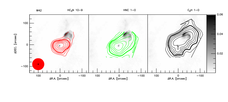
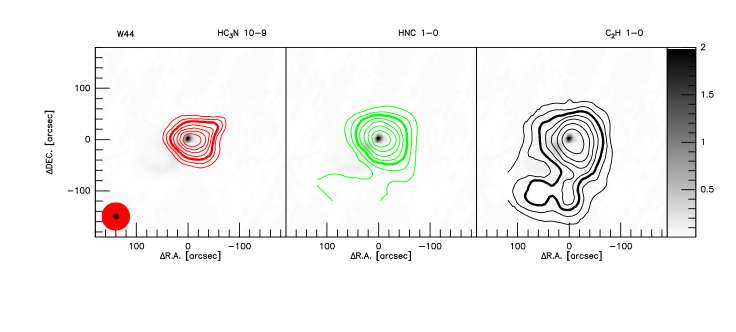
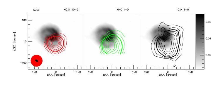
Figure 4: Contour maps of HC₃N 10-9 (left pannel), HNC 1-0 (middle pannel) and C₂H 1-0 (F = 3/2, 2 $\rightarrow$ 1/2, 1) (right pannel) integrated intensity superimposed on its 8.4 or 4.8 GHz continuum map in gray scale. (A color version of this figure is available in the online journal.)

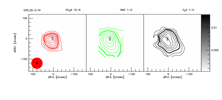
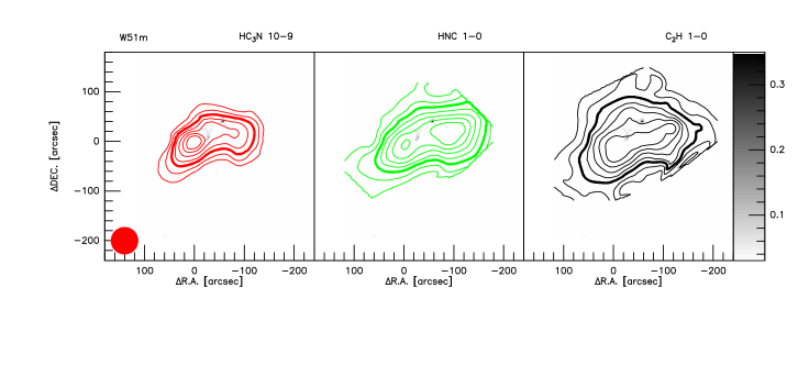
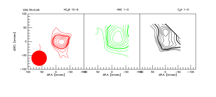
Figure 5: Contour maps of HC₃N 10-9 (left pannel), HNC 1-0 (middle pannel) and C₂H 1-0 (F = 3/2, 2 $\rightarrow$ 1/2, 1) (right pannel) integrated intensity superimposed on its 8.4 or 4.8 GHz continuum map in gray scale. (A color version of this figure is available in the online journal.)

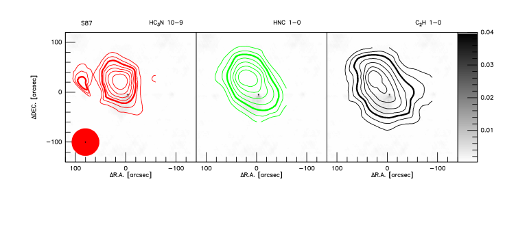
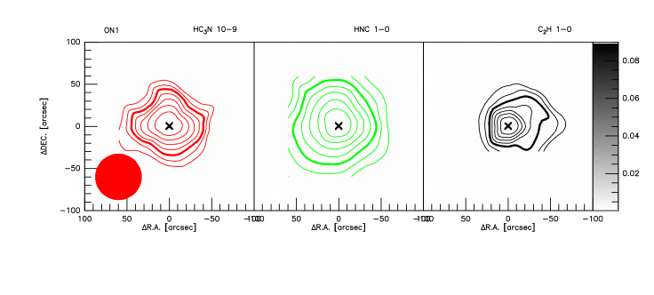
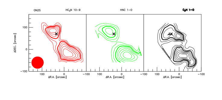
Figure 6: Contour maps of HC₃N 10-9 (left pannel), HNC 1-0 (middle pannel) and C₂H 1-0 (F = 3/2, 2 $\rightarrow$ 1/2, 1) (right pannel) integrated intensity superimposed on its 8.4 or 4.8 GHz continuum map in gray scale. (A color version of this figure is available in the online journal.)

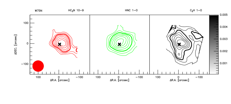
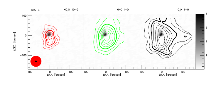
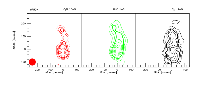
Figure 7: Contour maps of HC₃N 10-9 (left pannel), HNC 1-0 (middle pannel) and C₂H 1-0 (F = 3/2, 2 $\rightarrow$ 1/2, 1) (right pannel) integrated intensity superimposed on its 8.4 or 4.8 GHz continuum map in gray scale. (A color version of this figure is available in the online journal.)

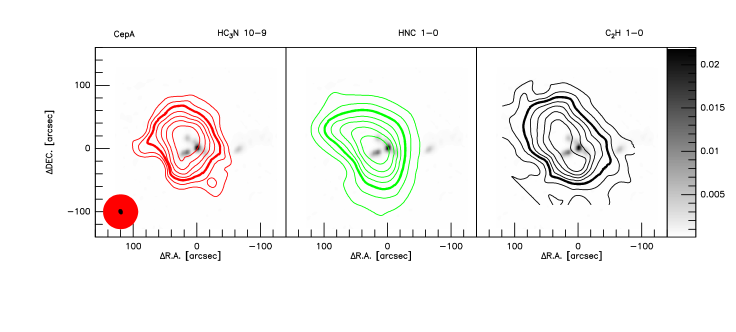
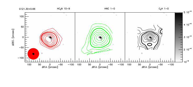
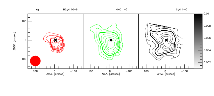
Figure 8: Contour maps of HC₃N 10-9 (left pannel), HNC 1-0 (middle pannel) and C₂H 1-0 (F = 3/2, 2 $\rightarrow$ 1/2, 1) (right pannel) integrated intensity superimposed on its 8.4 or 4.8 GHz continuum map in gray scale. (A color version of this figure is available in the online journal.)

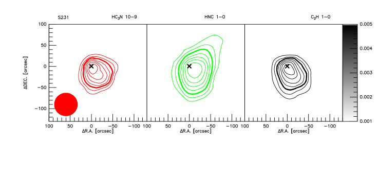
Figure 9: Contour maps of HC₃N 10-9 (left pannel), HNC 1-0 (middle pannel) and C₂H 1-0 (F = 3/2, 2 $\rightarrow$ 1/2, 1) (right pannel) integrated intensity superimposed on its 8.4 or 4.8 GHz continuum map in gray scale. (A color version of this figure is available in the online journal.)

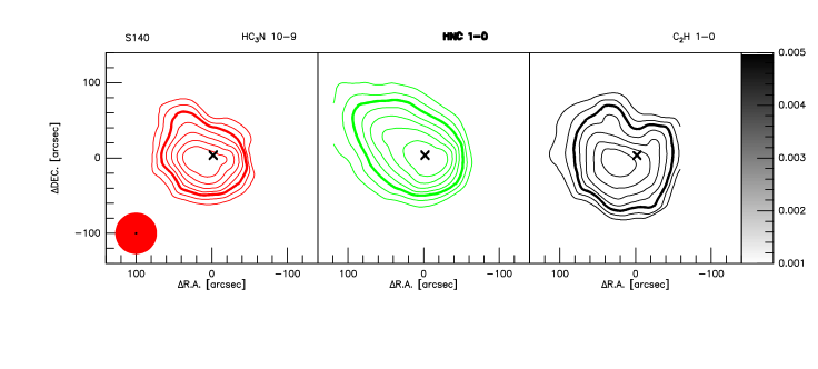
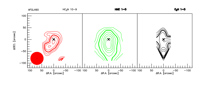
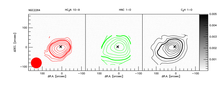
Figure 10: Figure 2 continued. (A color version of this figure is available in the online journal.)

Figure 13: Observed spectra of C₂H 1-0 toward Cep A, averaged over the whole emitting region.

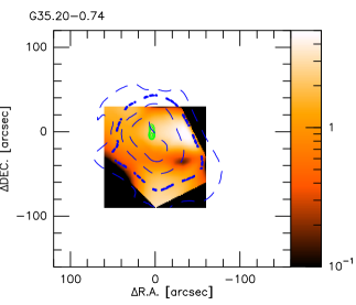
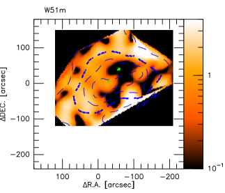
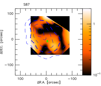
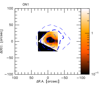
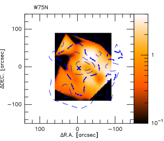
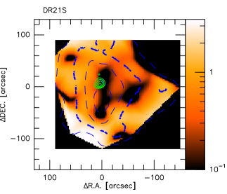
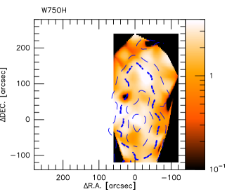
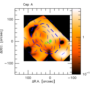
Figure 15: Contour maps C₂H 1-0 (J = 3/2$\rightarrow$1/2, F = 2$\rightarrow$1) (dashed line) integrated intensity and radio continuum emission (solid line) superimposed on the optical depth of C₂H 1-0 (J = 3/2$\rightarrow$1/2, F = 2$\rightarrow$1) in gray scale. (A color version of this figure is available in the online journal.)

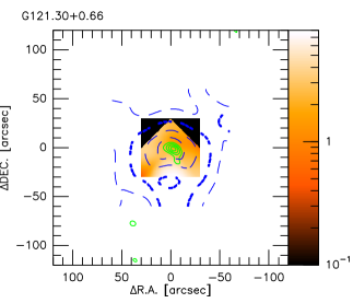
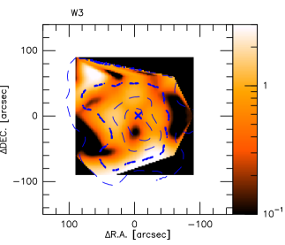
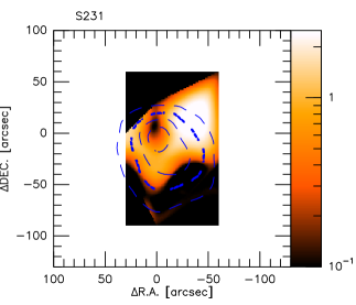
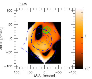
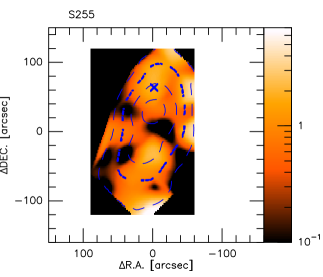
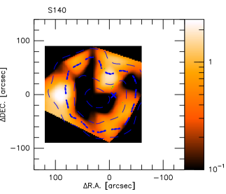
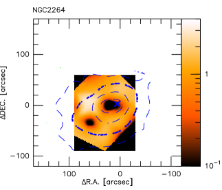
Figure 16: Contour maps C₂H 1-0 (J = 3/2$\rightarrow$1/2, F = 2$\rightarrow$1) (dashed line) integrated intensity and radio continuum emission (solid line) superimposed on the optical depth of C₂H 1-0 (J = 3/2$\rightarrow$1/2, F = 2$\rightarrow$1) in gray scale. (A color version of this figure is available in the online journal.)

References

- Alfven (1943) Alfvn, H. 1943, Ark.Mat.Astr.och.Fys., 29B, 2
- Arquilla et al. (1986) Arquilla, R. & Goldsmith, P. F. 1986, ApJ, 303, 356
- Bally et al. (1983) Bally, J. & Predmore, R. 1983, ApJ, 265, 778
- Barsony (1989) Barsony, M. 1989, ApJ, 345, 268
- Baxter (2009) Baxter, E. J., Covey, K. R., Muench, A. A. et al. 2009, AJ, 138, 963
- Bergin et al. (1996) Bergin, E. A., Snell, R. L. & Goldsmith, P. F. 1996, ApJ, 460, 343
- Bergin et al. (1997) Bergin, E. A., Ungerechts, H. & Goldsmith, P. F. 1997, ApJ, 482, 267
- Bergin et al. (2007) Bergin, E. A. & Tafalla, M. 2007, ARA&A, 45, 339
- Bertoldi et al. (1992) Bertoldi, F. & McKee, C. F. 1992, ApJ, 395, 140
- Blitz et al. (1982) Blitz, L., Fich, M. & Stark, A. A. 1982, ApJS, 49, 183
- Blitz et al. (1993) Blitz, L. 1993, in Protostars & Planets III, ed. E. H. Levy & J. I. Lunine (Tucson: Univ. Arizona Press), 125
- Brand et al. (1993) Brand, J. & Blitz, L. 1993, A&A, 275, 67
- Braz et al. (1983) Braz, M. A. & Epchtein, N. 1983, A&A, 54, 167
- Bourke et al. (2004) Bourke, T. L. & Goodman, A. A. 2004, IAUS, 221, 83
- Beuther et al. (2008) Beuther, H., Semenov, D., Henning, T. & Linz, H. 2008, ApJ, 675, L33
- Caselli et al. (2002) Caselli, P., Benson, P. J., Myers, P. C. & Tafalla, M., 2002, ApJ, 572, 238
- Cesaroni et al. (1988) Cesaroni, R., Palagi,, F., Felli, M. et al. 1988, A&AS, 76, 445
- Chung et al. (1991) Chung, H. S., Kameya, O. & Morimoto, M. 1991, JKAS, 24, 217
- Churchwell et al. (2002) Churchwell, E. 2002, ARA&A, 40, 27
- Churchwell et al. (2010) Churchwell, E., Sievers, A. & Thum, C. 2010, A&A, 513, 9
- Crutcher et al. (1996) Crutcher, R. M., Roberts, D. A., Mehringer, D. M. & Troland, T. H. 1996, ApJ, 462, L79
- Crutcher et al. (1999) Crutcher, R. M. 1999, ApJ, 520, 706
- Codella et al. (1997) Codella, C., Test, L. & Cesaroni, R. 1997, 325, 282
- Cygnowski et al. (2003) Cygnowski, C. J., Reid, M. J., Fish, V. L. & Ho, P. T. P. 2003, ApJ, 596, 344
- Dent et al. (1988) Dent, W. R. F., Macdonald, G. H. & Andersson, M. 1988, MNRAS, 235, 1397
- Downes et al. (1980) Downes, D., Wilson, T. L., Bieging, J. & Wink, J. 1980, A&A, 91, 186
- Falgarone et al. (2008) Falgarone, E., Troland, T. H., Crutcher, R. M. & Paubert, G. 2008, A&A, 487, 247
- Fermi et al. (1949) Fermi, E. 1949, PhysRev., 75, 1169
- Fleck et al. (1981) Fleck, R. C., Jr., & Clark, F. O. 1981, ApJ, 245, 898
- Gao et al. (2004a) Gao, Y., & Solomon, P. M. 2004a, ApJ, 606, 271
- Gao et al. (2004b) Gao, Y. & Solomon, P. M. 2004b, ApJS, 152, 63
- Gaume et al. (1993) Gaume, R. A., Johnston, K. J. & Wilson, T. L. 1993, ApJ, 417, 645
- Genzel et al. (1977) Genzel, R. & Downes, D. 1977, A&AS, 30, 145
- Girart et al. (2009) Girart, J. M., Beltran, M. T., Zhang, Q. Z., Rao, R. & Estalella, R. 2009, Science, 324, 1408
- Goodman et al. (1993) Goodman, A. A., Benson, P. J., Fuller, G. A. & Myers, P. C. 1993, ApJ, 406, 528
- Gwenlan et al. (2000) Gwenlan, C., Ruffle, D. P., Viti, S. et al. 2000, A&A, 354, 1127
- Higuchi et al. (2010) Higuchi, A. E., Kurono, Y., Saito, M. & Kawabe, R. 2010, ApJ, 719, 1813
- Hirota et al. (2008) Hirota, T., Ando, K., Bushimata, T. et al. 2008, PASJ, 60, 961
- Huggins et al. (1984) Huggins, P. J., Carlson, W. J. & Kinney, A. L. 1984, A&A, 133, 347
- Hunter et al. (1994) Hunter, T. R., Taylor, G. B., Felli, M. & Tofani, G. 1994, A&A, 284, 215
- Imara et al. (2011) Imara, N. & Blitz, L. 2011, ApJ, 732, 78
- Israel et al. (1978) Israel, F. P. & Felli, M. 1978, A&A, 63, 325
- Keto et al. (1987) Keto, E. R., Ho, P. T. P. & Haschick, A. D. 1987, ApJ, 318, 712
- Kurtz (2000) Kurtz, S. E. 2000, Rev. Mexicana Astron. Astrofits. Ser. Conf., 9, 169
- Kurtz (2002) Kurtz, S. E. & Franco, J. 2002, Rev. Mexicana Astron. Astrofits. Ser. Conf., 12, 16
- Lai (2001) Lai, S. P., Crutcher, R. M., Girart, J. M. & Rao, R. 2001, ApJ, 561, 864
- Larson (1981) Larson, R. B. 1981, MNRAS, 194, 809
- Leppanen (1998) Leppnen, K., Liljestrm, T. & Diamond, P. 1998, ApJ, 507, 909
- Liu (2010) Baobab Liu, H., Ho, P. T. P., Zhang, Q., Keto, E., Wu, J. W. & Liu, H. B. 2010, ApJ, 722, 262
- Machida (2005) Machida, M. N., Matsumoto, T., Tomisaka, K. & Hanawa, T. 2005, MNRAS, 362, 369
- Mardones et al. (1997) Mardones, D., Myers, P. C., Tafalla, M. et al. 1997, ApJ, 489, 719
- Matthews et al. (1983) Matthews, H. E. & Spoelstra, T. A. T. 1983, A&A, 126, 433
- Meier et al. (2005) Meier, D. S., & Turner, J. L. 2005, ApJ, 618, 259
- Mellema et al. (2006) Mellema, G., Arthur, S. J., Henney, W. J., Iliev, I. T. & Shapiro, P. R. 2006, ApJ, 647, 397
- Mellon et al. (2009) Mellon, R. & Li, Z. Y. 2009, ApJ, 698, 922
- Mestel et al. (1984) Mestel, L., & Paris, R. B. 1984, A&A, 136, 98
- Meyer et al. (1988) Meyer, P . C. & Goodman, A. A. 1988, ApJ, 329, 392
- Morris et al. (1975) Morris, M., Turner, B. E., Palmer, P. & Zuckerman, B. 1976, ApJ, 205, 82
- Morris et al. (1976) Morris, M., Snell, R. L. & Vanden Bout, P. 1977, ApJ, 216, 738
- Mouschovias et al. (1976) Mouschovias, T. Ch. & Spitzer, L. Jr. 1976, ApJ, 210, 326
- Mouschovias et al. (1979) Mouschovias, T. Ch. & Paleologou, E. V. 1979, ApJ, 230, 204
- Mueller et al. (2002) Mueller, K. E., Shirley, Y. L., Evans, N. J. II, & Jacobson, H. R. 2002, ApJS, 143, 469
- Padovani et al. (2009) Padovani, M., Walmsley, C. M., Tafalla, M. et al. 2009, A&A, 505, 1199
- Pardo et al. (2004) Pardo, J. R., Cernicharo, J. & Goicoechea, J. R. 2004, ApJ, 615, 495
- Philips et al. (1979) Philips, T. G., Huggins, P. J., Wannier, P. G. & Scville, N. Z. 1979, ApJ, 231, 720
- Philips (1999) Philips, J. P., 1999, A&AS, 134, 241
- Pirogov (2003) Pirogov, L., Zinchenko, I., Caselli, P. et al. 2003, A&A, 405, 639
- Plume (1992) Plume, R., Jaffe, D. T. & Evans II, N. J. 1992, ApJS, 78, 505
- Quireza et al. (2006) Quireza, C., Rood, R. T., Balser, D. S. & Bania, T. M. 2006, ApJS, 165, 338
- Reid et al. (2010) Reid, M. J., Menten, K. M., Zheng, X. W. et al. 2009, ApJ, 700, 137
- Rengarajan et al. (1996) Rengarajan, T. N. & Ho, P. T. P. 1996, ApJ, 465, 363
- Rodriguez et al. (1998) Rodriguez-Franco, A., Martin-Pintado, J. & Fuente, A. 1998, A&A, 329, 1097
- Rosolowsky et al. (2003) Rosolowsky, E., Engargiola, G., Plambeck, R., & Blitz, L. 2003, ApJ, 599, 258
- Rygl et al. (2010) Rygl, K. L. J., Brunthalaer, A., Reid, M. J. et al. 2010, A&A, 511, A2
- Sato et al. (2010) Sato, M., Reid, M. J., Brunthaler & Menten, K. M. 2010, ApJ, 720, 1055
- Schneider et al. (2010) Schneider, N., Csengeri, T., Bontemps, S. et al. 2010, A&A, 520, 49
- Shi et al. (2010) Shi, H., Zhao, J. H. & Han, J. L. 2010, ApJ, 710, 843
- Shirley et al. (2003) Shirley, Y. L., Evans, N. J., Young, K. S., Knez, C. & Jaffe, D. T., 2003, ApJS, 149, 375
- Snell et al. (1984) Snell, R. L., Scoville, N. Z., Sanders, D. B., & Erickson, N. R. 1984, ApJ, 284, 176
- Solomon et al. (1987) Solomon, P. M., Rivolo, A. R., Barret, J. & Yahil, A. 1987, ApJ, 319, 370
- Spitzer (1978) Spitzer, L. Jr. 1978, Physical Processes in the Interstellar Medium (New York: John Wiley and Sons)
- Sun et al. (2009) Sun, Y. & Gao, Y. 2009, MNRAS, 392, 170
- Tak et al. (2005) van der Tak, F. F. S. & Menten K. M. 2005, A&A, 437, 947
- Tomisaka et al. (1988) Tomisaka, K., Ikeuchi, S. & Nakamura, T. 1988, ApJ, 335, 239
- Tucker et al. (1974) Tucker, K. D., Kutner, M. L., & Thaddeus, P. 1974, ApJ, 193, L115
- Tucker et al. (1978) Tucker, K. D. & Kutner, M. L. 1978, ApJ, 222, 859
- Turner et al. (1971) Turner, B. E. 1971, ApJ, 163, L35
- van dishoeck et al. (1998) van Dishoeck, E. F. & Blake, G. A. 1998, ARA&A, 36, 317
- valtts et al. (2000) Val’tts, I. E., Ellingsen, S. P., Slysh, V. I., Kalenskii, S. V., Otrupcek, R. & Larionov, G. M. 2000, MNRAS, 317, 315
- vazquez et al. (2011) Vzquez-Semadeni, E., Banerjee, R., Gmez, G. C. et al. 2011, MNRAS, 414, 2511
- Walsh et al. (2010) Walsh, A. J., Thorwirth, S., Beuther, H., & Burton, M. G. 2010, MNRAS, 404, 1396
- Weise et al. (2010) Weise, P., Launhardt, R., Setiawan, J. & Henning, T. 2010, A&A, 517, 88
- Wood et al. (1989) Wood, D. O. S. & Churchwell, E. 1989, ApJS, 69, 831
- Wyrowski et al. (2003) Wyrowski, F., Schilke, P., Thorwirth, S., Menten, K. M. & Winnewisser, G. 2003, ApJ, 586, 344
- Wu et al. (2010) Wu, J. W., Evans, N. J., Shirley, Y. L. & Knez, C. 2010, ApJS, 188, 313
- Zhang et al. (2011) Zhang, S. B., Yang, J., Xu, Y. et al. 2011, ApJS, 193, 10
- Zheng et al. (1985) Zheng, X. W., Ho, P. T. P., Reid, M. J. & Schneps, M. H. 1985, ApJ, 293, 522
- Zheng et al. (1996) Zheng, X. W. & Huang, Y. F. 1996, Acta Astrophys. Sin., 16, 271
- Zinchenko (1994) Zinchenko, I., Forsstroem, V., Lapinov, A. & Mattila, K. 1994, A&A, 288, 601
- Zinchenko (1995) Zinchenko, I. 1995, A&A, 3033, 554
- Zinchenko et al. (1998) Zinchenko, I., Pirogov, L., Toriseva, M. 1998, A&AS, 133, 337
- Zinnecker et al. (2007) Zinnecker, H. & Yorke, H. W. 2007, ARA&A, 45, 481
- zuckerman (1973) Zuckerman, B. 1973, ApJ, 183, 863