∎
22email: zhangzk@lsec.cc.ac.cn
Sobolev seminorm of quadratic functions with applications to derivative-free optimization ††thanks: Partially supported by Chinese NSF grants 10831006, 11021101, and CAS grant kjcx-yw-s7.
Abstract
This paper studies the Sobolev seminorm of quadratic functions. The research is motivated by the least-norm interpolation that is widely used in derivative-free optimization. We express the seminorm of a quadratic function explicitly in terms of the Hessian and the gradient when the underlying domain is a ball. The seminorm gives new insights into least-norm interpolation. It clarifies the analytical and geometrical meaning of the objective function in least-norm interpolation. We employ the seminorm to study the extended symmetric Broyden update proposed by Powell. Numerical results show that the new thoery helps improve the performance of the update. Apart from the theoretical results, we propose a new method of comparing derivative-free solvers, which is more convincing than merely counting the numbers of function evaluations.
Keywords:
Sobolev seminorm Least-norm interpolation Derivative-free optimization Extended symmetric Broyden updateMSC:
90C56 90C30 65K051 Motivation and Introduction
Consider an unconstrained derivative-free optimization problem
| (1) |
where is a real-valued function whose derivatives are unavailable. Problems of this type have numerous applications. For instance, they have been employed to solve the helicopter rotor blade design problem booker1998managing ; booker1998optimization ; booker1999rigorous , the ground water community problems hemker2006derivative ; fowler2008comparison , and the problems in biomedical imaging oeuvray2005trust ; oeuvray2007new .
Many algorithms have been developed for problem (1). For example, direct search methods (see Wright wright1996direct , Powell powell1998direct , Lewis, Torczon, and Trosset lewis2000direct , and Kolda, Lewis, and Torczon kolda2003optimization for reviews), line search methods without derivatives (see Stewart stewart1967modification for a quasi-Newton method using finite difference; see Gilmore and Kelley gilmore1995implicit , Choi and Kelley choi2000superlinear , and Kelley kelley2002brief ; kelley2011implicit for Implicit Filtering method, a hybrid of quasi-Newton and grid-based search; see Diniz-Ehrhardt, Martínez, and Raydán diniz2008derivative for a derivative-free line search technique), and model-based methods (for instance, a method by Winfield winfield1973function , COBYLA by Powell COBYLA , DFO by Conn, Scheinberg, and Toint CoScTo97a ; Conn97recentprogress ; Conn98DFOPractice , UOBYQA by Powell Powell2000uobyqa , a wedge trust region method by Marazzi and Nocedal marazzi2002wedge , NEWUOA and extensions by Powell Powell2004newuoa ; Powell2008NEWUOAdev ; powell2009bobyqa ; powell2012beyond , CONDOR by Vanden Berghen and Bersini berghen2005condor , BOOSTERS by Oeuvray and Bierlaire oeuvray2008derivative , ORBIT by Wild, Regis, and Shoemaker wild2008orbit , MNH by Wild SMW08MNH , and a recent algorithm using sparse low degree model by Bandeira, Scheinberg, and Vicente bandeira2010computation ). We refer the readers to the book by Brent brent1973algorithms , the one by Kelley kelley1999iterative , and the one by Conn, Scheinberg, and Vicente Conn:2009:IntroDFO for extensive discussions and the references therein.
Multivariate interpolation has been acting as a powerful tool in the design of derivative-free optimization methods. The following quadratic interpolation plays an important role in Conn and Toint CoTo96a , Conn, Scheinberg, and Toint CoScTo97a ; Conn97recentprogress ; Conn98DFOPractice , Powell PowellLFNU ; Powell2004newuoa ; Powell2008NEWUOAdev ; powell2009bobyqa ; powell2012beyond , and Custódio, Rocha, and Vicente custodio2010incorporating :
| (2) |
where is the linear space of polynomials with degree at most two in variables, is a specific point in , is a nonnegative constant, is a finite set of interpolation points in , and is a function111Notice that is not always equal to the objective function , which is the case in Powell PowellLFNU ; Powell2004newuoa ; Powell2008NEWUOAdev ; powell2009bobyqa ; powell2012beyond . See Section 2 for details. on . We henceforth refer to this type of interpolation as least-norm interpolation.
The objective function of problem (2) is interesting. It is easy to handle, and practice has proved it successful. The main purpose of this paper is to provide a new interpretation of it. Our tool is the Sobolev seminorm, which is classical in PDE theory but may be rarely noticed in nonlinear optimization. We will give new insights into some basic questions about the objective function in (2). For example, what is the exact analytical and geometrical meaning of this objective? Why to combine the Frobenius norm of the Hessian and the -norm of the gradient? What is the meaning of the parameters and ?
This paper is organized as follows. Section 2 introduces the applications of least-norm interpolation in derivative-free optimization. Section 3 presents the main theoretical results. We first study the seminorm of quadratic functions, and then employ the seminorm to investigate least-norm interpolation. The questions listed above are answered in Section 3. Section 4 applies the theory obtained in Section 3 to study the extended symmetric Broyden update proposed by Powell powell2012beyond . We show an easy and effective way to improve the performance of the update. Section 5 concludes our discussion.
The main contributions of the paper lie in Section 3 and Section 4. Besides the theoretical results, the numerical experience in Section 4 is also a highlight. We propose a new method of testing derivative-free solvers by introducing statistics into the numerical experiments. See Subsection 4.3 for details.
A remark on notation. We use the notation
| (3) |
for the bilevel programming problem
| (4) |
2 Least-Norm Interpolation in Derivative-Free Optimization
Least-norm interpolation has successful applications in derivative-free optimization, especially in model-based algorithms. These algorithms typically follow trust-region methodology conn2000tr ; powell2003trust . On each iteration, a local model of the objective function is constructed, and then it is minimized within a trust-region to generate a trial step. The model is usually a quadratic polynomial constructed by solving an interpolation problem
| (5) |
where, as stated in problem (1), is the objective function, and is an interpolation set. To determine a unique quadratic polynomial by problem (5), the size of needs to be at least , which is prohibitive when is big. Thus we need to consider underdetermined quadratic interpolation. In that case, a classical strategy to take up the remaining freedom is to minimize some functional subject to the interpolation constraints, that is to solve
| (6) |
being some functional on . Several existing choices of lead to least-norm interpolation, directly or indirectly. Here we give some examples.
Conn and Toint CoTo96a suggests the quadratic model that solves
| (7) |
where is a specific point in (the center of the trust-region they use). Problem (7) is a least-norm interpolation problem with .
Conn, Scheinberg, and Toint CoScTo97a ; Conn97recentprogress ; Conn98DFOPractice builds a quadratic model by solving
| (8) |
It is considered as the best general strategy for the DFO algorithm to select a unique model from the pool of the possible interpolation models Conn98DFOPractice . Wild SMW08MNH also works with the model defined by (8). Problem (8) is a least-norm interpolation problem with . Conn, Scheinberg, and Vicente Conn:2009:IntroDFO explains the motivation for (8) by the following error bounds of quadratic interpolants.
Theorem 2.1
Conn:2009:IntroDFO Suppose that the interpolation set () is contained in a ball (), and the matrix
| (9) |
has rank . If is continuously differentiable on , and is Lipschitz continuous on with constant , then for any quadratic function satisfying the interpolation constraints (5), it holds that
| (10) |
and
| (11) |
In light of Theorem 2.1, minimizing some norm of will help improve the approximation of gradient and function value. Notice that appears in (10–11) with 2-norm rather than Frobenius norm.
Powell PowellLFNU ; Powell2004newuoa ; Powell2008NEWUOAdev introduce the symmetric Broyden update to derivative-free optimization, and it is proposed to solve
| (12) |
to obtain a model for the current iteration, provided that is the quadratic model used in the previous iteration. Problem (12) is essentially a least-norm interpolation problem about . The symmetric Broyden update is motivated by least change secant updates dennis1979least in quasi-Newton methods. One particularly interesting advantage of the update is that, when is a quadratic function, approximates better than unless , being the model obtained by the update PowellLFNU ; Powell2004newuoa ; Powell2008NEWUOAdev .
Powell powell2012beyond proposes the extended symmetric Broyden update by adding a first-order term to the objective function of problem (12), resulting in
| (13) |
and being specifically selected parameters, nonnegative. Again, (13) can be interpreted as a least-norm interpolation about . Powell powell2012beyond motivates (13) by an algebraic example for which the symmetric Broyden update does not behave satisfactorily. We will study the extended symmetric Broyden update in Section 4.
Apart from model-based methods, least-norm interpolation also has applications in direct search methods. Custódio, Rocha, and Vicente custodio2010incorporating incorporates models defined by (8) and (12) into direct search. The authors attempt to enhance the performance of direct search methods by taking search steps based on these models. It is reported that (8) works better for their method, and their procedure provides significant improvements to direct search methods of directional type.
For more discussions about least-norm interpolation in derivative-free optimization, we refer the readers to Chapters 5 and 11 of Conn, Scheinberg, and Vicente Conn:2009:IntroDFO .
3 The Sobolev Seminorm of Quadratic Functions
In Sobolev space theory adams1975sobolev ; evans1998partial , the seminorm of a function over a domain is defined as
| (14) |
In this section, we give an explicit formula for the seminorm of quadratic functions when is a ball, and accordingly present a new understanding of least-norm interpolation. We prove that least-norm interpolation essentially seeks the quadratic interpolant with minimal seminorm over a ball. Theorem 3.1, Theorem 3.2, and Theorem 3.3 are the main theoretical results of this paper.
3.1 The Seminorm of Quadratic Functions
The seminorm of a quadratic function over a ball can be expressed explicitly in terms of its coefficients. We present the formula in the following theorem.
Theorem 3.1
Let be a point in , be a positive number, and
| (15) |
Then for any ,
| (16) |
where is the volume of the unit ball in .
Proof
Without loss of generality, we assume that . Let
| (17) |
Then
| (18) |
Because of symmetry, the integral of is zero. Besides,
| (19) |
Thus we only need to find the integral of . Now we assume that is diagonal (if not, apply a rotation). Denote the -th diagonal entry of by , and the -th coordinate of by . Then
| (20) |
To finish the proof, we show that
| (21) |
It suffices to justify (21) for the case and . First,
| (22) |
and, similarly,
| (23) |
Second, integration by parts shows that
| (24) |
Theorem 3.1 tells us that the seminorm of a quadratic function over a ball is closely related to a combination of and , being the center of , and the combination coefficients being determined by the radius of . This result is interesting for two reasons. First, it enables us to measure the overall magnitude of the gradient over a ball. This is nontrivial for a quadratic function, since its gradient is not constant. Second, it clarifies the analytical and geometrical meaning of combining the Frobenius norm of the Hessian and the 2-norm of the gradient, and enables us to select the combination coefficients according to the geometrical meaning.
3.2 New Insights into Least-Norm Interpolation
The seminorm provides a new angle of view to understand least-norm interpolation. For convenience, we rewrite the least-norm interpolation problem here and call it the problem :
| () |
We assume that the interpolation system
| (25) |
is consistent on , namely
| (26) |
With the help of Theorem 3.1, we see that the problem is equivalent to the problem
| () |
in some sense. The purpose of this subsection is to clarify the equivalence.
When , the equivalence is easy and we state it as follows.
It turns out that the least-norm interpolation problem with positive essentially seeks the interpolant with minimal seminorm over a ball. The geometrical meaning of and is clear now: is the center of the ball, and is the radius.
Now we consider the least-norm interpolation problem with . This case is particularly interesting, because it appears in several practical algorithms Conn98DFOPractice ; Powell2004newuoa ; SMW08MNH . Since may have multiple solutions when , we modify the definition of : from now on, is defined to be the bilevel least-norm interpolation problem
| () |
The new definition is reasonable, because the following proposition holds after the modification.
Proposition 1
Proof
The uniqueness of the solution is simple. First, the uniqueness of the Hessian and gradient is guaranteed by the convexity of the objective functional(s); then with the help of any one of the interpolation constraints, we find that the constant term is also unique.
In light of the uniqueness stated above, the convergence of is a corollary of the classical penalty function theory in nonlinear optimization (see, for instance, Theorem 12.1.1 of Fletcher Fletcher:1987:PMO ). ∎
Note that Proposition 2 implies the problem has a unique solution for each positive . Now we can state the relation between the problems and .
Theorem 3.3 indicates that, when , the least-norm interpolation problem seeks the interpolant with minimal seminorm over in the sense of limit. Thus Theorem 3.3 is the extension of Theorem 3.2 to the case .
The questions listed in Section 1 can be answered now. The meaning of the objective function in least-norm interpolation is to minimize the seminorm of the interpolant over a ball. The reason to combine the Frobenius norm of the Hessian and the 2-norm of the gradient is to measure the seminorm of the interpolant. The parameters and determines the ball where the seminorm is calculated, being the center and being the radius. When , we can interprete least-norm interpolation in the sence of limit.
4 On the Extended Symmetric Broyden Update
In this section, we employ the seminorm to study the extended symmetric Broyden update proposed by Powell powell2012beyond . As introduced in Section 2, the update defines to be the solution of
| (27) |
being the objective function, and being the model used in the previous trust-region iteration. When , it is the symmetric Broyden update studied by Powell PowellLFNU ; Powell2004newuoa ; Powell2008NEWUOAdev . We focus on the case . In Subsection 4.1, we interpret the update with the seminorm. In Subsection 4.2, we discuss the choices of and in the update, and show how to choose and according to their geometrical meaning. In Subsection 4.3, we test our choices of and through numerical experiments. It is worth mentioning that, the numerical experiments in Subsection 4.3 are designed in a special way in order to reduce the influence of computer rounding errors and obtain more convincing results.
4.1 Interpret the Update with the Seminorm
According to Theorem 3.2, problem (27) is equivalent to
| (28) |
where
| (29) |
Thus the extended symmetric Broyden update seeks the closest quadratic model to subject to the interpolation constraints, distance being measured by the seminorm .
Similar to the symmetric Broyden update, the extended symmetric Broyden update enjoys a very good approximation property when is a quadratic function, as stated in Proposition 2.
Proposition 2
Proof
Let , being any real number. Then is a quadratic function interpolating on , as is quadratic and interpolates it. The optimality of implies that the function
| (31) |
attains its minimum when is zero. Expanding , we obtain
| (32) |
Hence
| (33) |
Then we obtain (30) by considering .∎
In light of Theorem 3.1, equation (30) is equivalent to equation (1.9) of Powell powell2012beyond . Notice that equation (30) implies
| (34) |
In other words, approximates on better than unless .
4.2 Choices of and
Now we turn our attention to the choices of and in the update. Recall that the purpose of the update is to construct a model for a trust-region subproblem. As in classical trust-region methods, the trust region is available before the update is applied, and we suppose it is
| (35) |
the point being the trust-region center, and the positive number being the trust-region radius.
Powell powell2012beyond chooses and by exploiting the Lagrange functions of the interpolation problem (27). Suppose that , then the -th () Lagrange function of problem (27) is defined to be the solution of
| (36) |
being the Kronecker delta. In the algorithm of Powell powell2012beyond , is maintained in a way so that interpolates on except one point, say without loss of generality. Then the interpolation constraints can be rewritten as
| (37) |
Therefore the solution of problem (27) is
| (38) |
Hence plays a central part in the update. Thus Powell powell2012beyond chooses and by examining . Powell shows that, in order to make sure behaves well, the ratio should not be much larger than one, therefore is set to be throughout the calculation. The choice of is a bit complicated. The basic idea is to balance and . Thus is set to , where and are estimates of the magnitudes of and , respectively. See Powell powell2012beyond for details.
In Subsection 4.1, we have interpreted the extended symmetric Broyden update with the seminorm. The new interpretation enables us to choose and in a geometrical way. According to problem (28), choosing and is equivalent to choosing the ball . Let us think about the role that plays in the update. First, is the region where the update tries to preserve information from , by minimizing the change with respect to the seminorm . Second, is the region where the update tends to improve the model, as suggested by the facts (30) and (34) for quadratic objective function. Thus we should choose to be a region where the behavior of the new model is important to us. It may seem adequate to pick to be the trust region (35). But we prefer to set it bigger, because the new model will influence its successors via the least change update, and thereby influence subsequent trust-region iterations. Thus it is myopic to consider only the current trust region, and a more sensible choice is to let be the ball , being a positive number bigger than one333Since the trust-region radii of the subsequent iterations vary dynamically according to the degree of success, there should be more elaborate ways to define the domain adaptively. The definition given here might be the simplest one, and is enough for our experiment.. Moreover, we find in practice that it is helpful to require . Thus our choice of is
| (39) |
where
| (40) |
Consequently, we set
| (41) |
Therefore our choice of coincides with Powell’s, but the choice of is different.
4.3 Numerical Results
With the help of the seminorm, we have proposed a new method of choosing for the extended symmetric Broyden update. In this subsection we test the new through numerical experiments, and make comparison with the one by Powell powell2012beyond .
Powell powell2012beyond implements a trust-region algorithm based on the extended symmetric Broyden update in Fortran 77. We modify this code to get two solvers as follows for comparison.
-
a.)
ESYMBP: is chosen according to Powell powell2012beyond , as described in the second paragraph of Subsection 4.2.
- b.)
In the code of Powell powell2012beyond , the size of the interpolation set is kept unchanged throughout the computation, and the user can set it to be any integer between and . We chose as recommended. The terminate criterion of this code is determined by a parameter named RHOEND. RHOEND acts as the final trust-region radius in the code, and its magnitude usually agrees with the precision of the computational solution. We tested ESYMBPand ESYMBSwith RHOEND , and , to observe the performance of the solvers under different requirements of solution precision. The code of Powell powell2012beyond is capable of solving problems with box constraints. We set the bounds to infinity since we are focusing on unconstrained problems.
We assume that evaluating the objective function is the most expensive part for optimization without derivatives. Thus we might compare the performance of different derivative-free solvers by simply counting the numbers of function evaluations they use until termination, provided that they have found the same minimizer to high accuracy. However, this is inadequate in practice, because, according to our numerical experiences, computer rounding errors could substantially influence the number of function evaluations. Powell Powell2004newuoa presents a very interesting example for this phenomenon. In the example, the computational result of a test problem was influenced dramatically by the order of variables. But the code under test (NEWUOA) was mathematically independent of variables’ order. Thus the differences in the results are due entirely to computer rounding errors. Please see Section 8 of Powell Powell2004newuoa for details of the example.
We test the solvers ESYMBS and ESYMBP with the following method, in order to observe their performance in a relatively reliable way, and to inspect their stability with respect to computer rounding errors. The basic idea is from the numerical experiments of Powell powell2012beyond . Given a test problem with objective function and starting point , we randomly generate permutation matrices (), and let
| (42) |
Then we employ the solvers to minimize starting form . For solver , we obtain a vector , being the number of function evaluations required by for and . If the code of is mathematically independent of variables’ order (it is the case for ESYMBS and ESYMBP), then all the entries of are identical in theory. However, it is not the case in practice, and the differences are completely made by computer rounding errors. We compute the mean value and the standard deviation of vector :
| (43) |
and
| (44) |
When is reasonably large, estimates the average performance of solver on problem , and reflects the stability of solver with respect to computer rounding errors when solving problem . We may also compute the relative standard deviation of , namely,
| (45) |
to obtain a normalized measure of stability. By comparing these statistics, we can reasonably assess the solvers under consideration. We use in practice.
With the method addressed above, we tested ESYMBP and ESYMBS on 30 unconstrained test problems with alterable dimension. The problems are from CUTEr cuter and Powell Powell2004newuoa , with names listed in Table 1.
| ARGLINA | ARGLINB | ARGLINC | ARWHEAD | BDQRTIC |
| BROYDN3D | BRYBND | CHROSEN | COSINE | CURLY10 |
| CURLY20 | CURLY30 | DQRTIC | EDENSCH | EG2 |
| ENGVAL1 | FLETCBV2 | FREUROTH | GENBROWN | INTEGREQ |
| NONCVXUN | PENALTY1 | PENALTY2 | POWER | SCHMVETT |
| SPARSINE | SPARSQUR | SPHRPTS | TOINTGSS | VARDIM |
For each problem, we solved it for dimensions 6, 8, 10, 12, 14, and 16. We set the maximal number of function evaluations to be 1000. The experiments were carried out on a Thinkpad T400 laptop with Linux 2.6.33, and the compiler was gfortran in GCC 4.3.3.
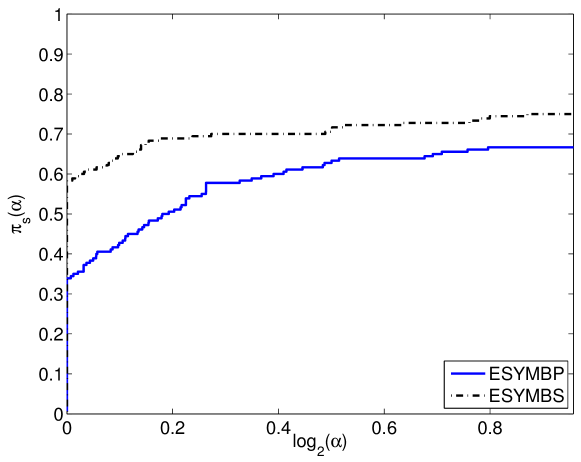
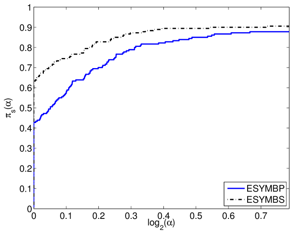
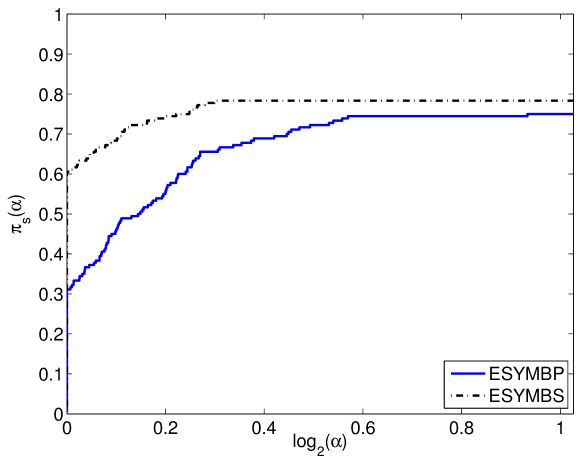
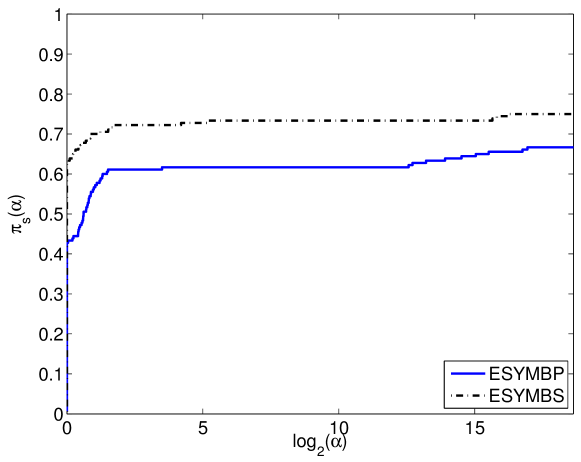
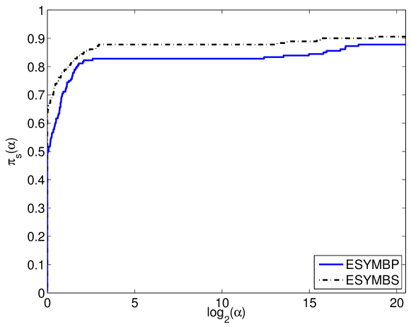
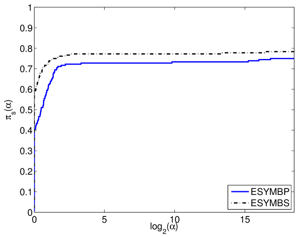
We visualize the results of our experiments by presenting the performance profiles dolan2002benchmarking of in Fig. 1, 2, and 3. The same as traditional performance profiles, the higher means the better. The profiles suggest that, in our experiments, ESYMBS performed better than ESYMBP in the sense of number of function evaluations. Moreover, ESYMBS also showed better stability than ESYMBP, with respect to computer rounding errors. To make the comparison, we present the performance profiles of in Fig. 4, 5, and 6. As before, the higher means the better. Thus the profiles support the conclusion that ESYMBS performed stabler than ESYMBP with respect to computer rounding errors.
From the results of our experiments, we conclude that the seminorm has suggested a better way of parameter selection for extended symmetric Broyden update, compared with the method given in Powell powell2012beyond . The new selection reduces the number of function evaluations in the resultant algorithm, and improves the solver’s stability with respect to computer rounding errors. Moreover, the new selection is much simpler and easier to understand than the one in Powell powell2012beyond .
4.4 A Remark on Extended Symmetric Broyden Update
It is interesting to ask whether the extended symmetric Broyden update can bring improvements to the original version in derivative-free optimization. Powell powell2012beyond studies this problem, and it turns out that the extended version rarely reduced the number of function evaluations. We have to point out that it is also the case when is selected with our method. However, some numerical experiments of Powell powell2012beyond suggested that the extended version might help to improve the convergence rate. It would be desirable to theoretically investigate the local convergence properties of the updates. We think it is still too early to draw any conclusion on the extended symmetric Broyden update, unless we could find strong theoretical evidence.
5 Conclusions
Least-norm interpolation has wide applications in derivative-free optimization. Motivated by its objective function, we have studied the Sobolev seminorm of quadratic functions. We gives an explicit formula for the seminorm of quadratic functions over balls. It turns out that least-norm interpolation essentially seeks a quadratic interpolant with minimal seminorm over a ball. Moreover, we find that the parameters and in the objective function determines the center and radius of the ball, respectively. These insights further our understanding of least-norm interpolation.
With the help of the new observation, we have studied the extended symmetric Broyden update (27) proposed by Powell powell2012beyond . Since the update calculates the change to the old model by a least-norm interpolation, we can interpret it with our new theory. We have discussed how to choose and for the update according to their geometrical meaning. This discussion leads to the same used by Powell powell2012beyond , and a very easy way to choose . According to our numerical results, the new works better than the one proposed by Powell powell2012beyond .
Our method of designing numerical tests seems reasonable. It provides a more reliable measurement of computation cost than simply counting the numbers of function evaluations, and meanwhile reflects the stability of solvers with respect to computer rounding errors. We hope this method can lead to better benchmarking of derivative-free solvers.
Acknowledgements.
The author thanks Professor M. J. D. Powell for providing references and codes, for kindly answering the author’s questions about the excellent software NEWUOA, and for the helpful discussions. Professor Powell helped improve the proofs of Theorem 3.1 and Proposition 2. The author owes much to his supervisor Professor Ya-Xiang Yuan for the valuable directions and suggestions. This work was partly finished during a visit to Professor Klaus Schittkowski at Universität Bayreuth in 2010, where the author has received pleasant support for research. The author thanks Humboldt Fundation for the financial assistance during this visit, and he is much more than grateful to Professor Schittkowski for his warm hospitality. The author appreciates the help of Professor Andrew R. Conn and an anonymous referee. Their comments have substantially improved the paper.References
- (1) Adams, R.A.: Sobolev spaces. Pure and applied mathematics. Academic Press (1975)
- (2) Bandeira, A.S., Scheinberg, K., Vicente, L.N.: Computation of sparse low degree interpolating polynomials and their application to derivative-free optimization. Mathematical Programming 134(1), 223–257 (2012)
- (3) Booker, A.J., Dennis, J.E., Frank, P.D., Serafini, D.B., Torczon, V., Trosset, M.W.: A rigorous framework for optimization of expensive functions by surrogates. Structural and Multidisciplinary Optimization 17(1), 1–13 (1999)
- (4) Booker, A.J., Dennis Jr, J.E., Frank, P., Serafini, D.B., Torczon, V., Trosset, M.W.: Optimization using surrogate objectives on a helicopter test example. PROGRESS IN SYSTEMS AND CONTROL THEORY 24, 49–58 (1998)
- (5) Booker, A.J., Frank, P., Dennis Jr, J.E., Moore, D.W., Serafini, D.B.: Managing surrogate objectives to optimize helicopter rotor design–further experiments. In: IN PROCEEDINGS OF THE SEVENTH AIAA/USAF/NASA/ISSMO SYMPOSIUM ON MULTIDISCIPLINARY ANALYSIS AND OPTIMIZATION (1998)
- (6) Brent, R.P.: Algorithms for minimization without derivatives. Prentice-Hall, Englewood Cliffs, New Jersey (1973)
- (7) Choi, T.D., Kelley, C.T.: Superlinear convergence and implicit filtering. SIAM Journal on Optimization 10(4), 1149–1162 (2000)
- (8) Conn, A.R., Gould, N.I.M., Toint, Ph.L.: Trust-region methods, MPS-SIAM series on optimization, vol. 1. Society for Industrial Mathematics (2000)
- (9) Conn, A.R., Scheinberg, K., Toint, Ph.L.: On the Convergence of Derivative-Free Methods for Unconstrained Optimization. In: M.D. Buhmann, A. Iserles (eds.) Approximation Theory and Optimization: Tributes to M. J. D. Powell, pp. 83–108. Cambridge University Press, Cambridge, United Kingdom (1997)
- (10) Conn, A.R., Scheinberg, K., Toint, Ph.L.: Recent progress in unconstrained nonlinear optimization without derivatives. Mathematical Programming 79, 397–414 (1997)
- (11) Conn, A.R., Scheinberg, K., Toint, Ph.L.: A derivative free optimization algorithm in practice. In: Proceedings of 7th AIAA/USAF/NASA/ISSMO Symposium on Multidisciplinary Analysis and Optimization. St. Louis, MO (1998)
- (12) Conn, A.R., Scheinberg, K., Vicente, L.N.: Introduction to Derivative-Free Optimization. Society for Industrial and Applied Mathematics, Philadelphia, PA, USA (2009)
- (13) Conn, A.R., Toint, Ph.L.: An Algorithm Using Quadratic Interpolation for Unconstrained Derivative Free Optimization. In: G. Di Pillo, F. Giannessi (eds.) Nonlinear Optimization and Applications, pp. 27–47. Kluwer Academic/Plenum Publishers, New York (1996)
- (14) Custódio, A.L., Rocha, H., Vicente, L.N.: Incorporating minimum frobenius norm models in direct search. Computational Optimization and Applications 46(2), 265–278 (2010)
- (15) Dennis Jr, J.E., Schnabel, R.B.: Least change secant updates for quasi-newton methods. Siam Review pp. 443–459 (1979)
- (16) Diniz-Ehrhardt, M.A., Martínez, J.M., Raydán, M.: A derivative-free nonmonotone line-search technique for unconstrained optimization. Journal of Computational and Applied Mathematics 219(2), 383–397 (2008)
- (17) Dolan, E.D., Moré, J.J.: Benchmarking optimization software with performance profiles. Mathematical Programming 91(2), 201–213 (2002)
- (18) Evans, L.C.: Partial differential equations. Graduate studies in mathematics. American Mathematical Society (1998)
- (19) Fletcher, R.: Practical Methods of Optimization, second edn. John Wiley & Sons, New York (1987)
- (20) Fowler, K.R., Reese, J.P., Kees, C.E., Dennis Jr, J.E., Kelley, C.T., Miller, C.T., Audet, C., Booker, A.J., Couture, G., Darwin, R.W.: Comparison of derivative-free optimization methods for groundwater supply and hydraulic capture community problems. Advances in Water Resources 31(5), 743–757 (2008)
- (21) Gilmore, P., Kelley, C.T.: An implicit filtering algorithm for optimization of functions with many local minima. SIAM Journal on Optimization 5, 269 (1995)
- (22) Gould, N.I.M., Orban, D., Toint, Ph.L.: CUTEr and SifDec: A constrained and unconstrained testing environment, revisited. ACM Transactions on Mathematical Software (TOMS) 29(4), 373–394 (2003)
- (23) Hemker, T., Fowler, K., Von Stryk, O.: Derivative-free optimization methods for handling fixed costs in optimal groundwater remediation design. In: Proc. of the CMWR XVI-Computational Methods in Water Resources, pp. 19–22 (2006)
- (24) Kelley, C.: Iterative methods for optimization, Frontiers in applied mathematics, vol. 18. Society for Industrial Mathematics (1999)
- (25) Kelley, C.T.: A brief introduction to implicit filtering. North Carolina State Univ., Raleigh, NC, CRSC Tech. Rep. CRSC-TR02-28 (2002)
- (26) Kelley, C.T.: Implicit filtering. Society for Industrial and Applied Mathematics (2011)
- (27) Kolda, T.G., Lewis, R.M., Torczon, V.: Optimization by direct search: New perspectives on some classical and modern methods. Siam Review pp. 385–482 (2003)
- (28) Lewis, R.M., Torczon, V., Trosset, M.W.: Direct search methods: then and now. Journal of Computational and Applied Mathematics 124(1), 191–207 (2000)
- (29) Marazzi, M., Nocedal, J.: Wedge trust region methods for derivative free optimization. Mathematical programming 91(2), 289–305 (2002)
- (30) Oeuvray, R.: Trust-region methods based on radial basis functions with application to biomedical imaging. Ph.D. thesis, ÉCOLE POLYTECHNIQUE FÉDÉRALE DE LAUSANNE (2005)
- (31) Oeuvray, R., Bierlaire, M.: A new derivative-free algorithm for the medical image registration problem. International Journal of Modelling and Simulation 27(2), 115–124 (2007)
- (32) Oeuvray, R., Bierlaire, M.: a derivative-free algorithm based on radial basis functions. In: International Journal of Modelling and Simulation (2008)
- (33) Powell, M.J.D.: A direct search optimization method that models the objective and constraint functions by linear interpolation. Advances in Optimization and Numerical Analysis pp. 51–67 (1994)
- (34) Powell, M.J.D.: Direct search algorithms for optimization calculations. Acta Numerica 7(1), 287–336 (1998)
- (35) Powell, M.J.D.: UOBYQA: unconstrained optimization by quadratic approximation. Tech. Rep. DAMTP NA2000/14, CMS, University of Cambridge (2000)
- (36) Powell, M.J.D.: On trust region methods for unconstrained minimization without derivatives. Mathematical programming 97(3), 605–623 (2003)
- (37) Powell, M.J.D.: Least frobenius norm updating of quadratic models that satisfy interpolation conditions. Mathematical Programming 100, 183–215 (2004)
- (38) Powell, M.J.D.: The NEWUOA software for unconstrained optimization without derivatives. Tech. Rep. DAMTP NA2004/08, CMS, University of Cambridge (2004)
- (39) Powell, M.J.D.: Developments of NEWUOA for minimization without derivatives. IMA Journal of Numerical Analysis pp. 649–664 (2008). DOI 10.1093/imanum/drm047
- (40) Powell, M.J.D.: The BOBYQA algorithm for bound constrained optimization without derivatives. Tech. Rep. DAMTP 2009/NA06, CMS, University of Cambridge (2009)
- (41) Powell, M.J.D.: Beyond symmetric Broyden for updating quadratic models in minimization without derivatives. Mathematical Programming pp. 1–26 (2012). DOI 10.1007/s10107-011-0510-y. URL http://dx.doi.org/10.1007/s10107-011-0510-y
- (42) Stewart III, G.: A modification of davidon’s minimization method to accept difference approximations of derivatives. Journal of the ACM (JACM) 14(1), 72–83 (1967)
- (43) Vanden Berghen, F., Bersini, H.: CONDOR, a new parallel, constrained extension of powell’s UOBYQA algorithm: Experimental results and comparison with the DFO algorithm. Journal of Computational and Applied Mathematics 181(1), 157–175 (2005)
- (44) Wild, S.M.: MNH: a derivative-free optimization algorithm using minimal norm Hessians. In: Tenth Copper Mountain Conference on Iterative Methods (2008)
- (45) Wild, S.M., Regis, R.G., Shoemaker, C.A.: ORBIT: Optimization by radial basis function interpolation in trust-regions. SIAM Journal on Scientific Computing 30(6), 3197–3219 (2008)
- (46) Winfield, D.H.: Function minimization by interpolation in a data table. IMA Journal of Applied Mathematics 12(3), 339 (1973)
- (47) Wright, M.H.: Direct search methods: Once scorned, now respectable. PITMAN RESEARCH NOTES IN MATHEMATICS SERIES pp. 191–208 (1996)