The Critical Coupling Likelihood Method: A new approach for seamless integration of environmental and operating conditions of gravitational wave detectors into gravitational wave searches.
Abstract
Any search effort for gravitational waves (GW) using interferometric detectors like LIGO needs to be able to identify if and when noise is coupling into the detector’s output signal. The Critical Coupling Likelihood (CCL) method has been developed to characterize potential noise coupling and in the future aid GW search efforts. By testing two hypotheses about pairs of channels, CCL is able to identify undesirable coupled instrumental noise from potential GW candidates. Our preliminary results show that CCL can associate up to of observed artifacts with , to local noise sources, while reducing the duty cycle of the instrument by . An approach like CCL will become increasingly important as GW research moves into the Advanced LIGO era, going from the first GW detection to GW astronomy.
pacs:
04.80.Nn, 95.55.Ym, 07.60.Ly1 Introduction
Detectable gravitational waves (GWs) are perturbations of the local space-time metric which are associated with distant astrophysical phenomena. According to general relativity, these perturbations travel at the speed of light and are generated by astronomical scale masses with time varying quadrupolar and higher moments. The main goal of the Laser Interferometric Gravitational-Wave Observatory (LIGO) is to detect GWs and use this information to study the astrophysics associated with those sources [1].
The LIGO detectors are now undergoing a major upgrade. This upgrade will increase the instrument’s sensitivity, extending the binary neutron star (BNS) observational range from the current to [2]. This change in the observational volume should increase the expected observable rate of GW signals. Using an improved network of GW detectors, one can expect BNS detection rates to improve from to [3, 4]. In order to achieve such sensitivity, LIGO instruments will be completely refitted with advanced components and control systems. This new configuration is called Advanced LIGO (aLIGO). During the aLIGO operational era, the first GW detection will mark the beginning of gravitational wave astronomy.
The first GW detection will be thoroughly reviewed. In an era of regular GW detection, human resource costly procedures such as the traditional follow-ups and post-facto data quality (DQ) studies should be relied on infrequently; the state of the instrument, and hence the DQ have a significant impact on the effectiveness of LIGO’s GW searches. Current DQ efforts identify epochs of questionable data quality. The DQ is analyzed in subsets, starting with the best data available, and epochs of decreasing quality data are added to the analysis to increase the effective observing time of the GW detector [5, 6]. Upon completion or near the end of an analysis the results are either disregarded immediately or further scrutinized during the follow-up procedure, to determine if the potential GW candidate is the signature of an actual GW signal [7, 8].
In this paper we are proposing a new method, the Critical Coupling Likelihood method, to investigate instrumental behavior and DQ. This method is intended to quantify instrumental operating conditions. We will also remark on how this information could be integrated into future GW searches. The CCL method uses the same sources of information as current DQ investigation methods, though it is a significant departure from those methods [9]. LIGO’s current DQ methods have been invaluable and used in some form for all previous science runs for studying instrumental behavior and noise coupling. These existing methods became the standard for investigating LIGO’s DQ but in an aLIGO era they may no longer be optimal methods for future DQ studies. Significant revisions to these methods or new methods may be needed in order to make DQ investigations manageable in an aLIGO era [10].
Understanding preponderant non-Gaussian noise sources is compulsory so that one can isolate them during the search process without unnecessarily compromising the instrument duty cycle. These noise sources generate transients which are typically the result of a local influence on the instrument, and can lead to false GW candidates. In order to uncover the sources of these transients in LIGO data there are a large number of sensors which are collectively referred to as physical and environmental monitors (PEMs).
LIGO records information about the detector’s operating environment and the control systems of the interferometer. This information is used to determine if a specific sampled time from the instrument’s GW output signal is or is not a noise transient in the system. In order to accomplish this, each of the sensors are analyzed individually to identify departures from their nominal behavior. The results of this analysis could be used to identify and discard noise transients occurring during times of questionable data quality as part of a GW search [11].
We propose to improve GW searches by applying our method, the Critical Coupling Likelihood (CCL) method. This method is expected to integrate information about the instrument’s operating condition and its environment directly into a search.
2 The Critical Coupling Likelihood
CCL is a statistical method intended to quantitatively identify as many avenues of environmental-to-instrumental coupling as possible. To accomplish this, the CCL method is based on time coincidence between event pairs from preselected data streams. This pairing is done between the GW data stream (GW channel) and an auxiliary sensor data stream (sensor channel). This method is intended to distinguish between real coincidences (coupling) and accidental coincidences, which are coincidences unlikely to be of physical interest.
It is reasonable to expect that any sensor will have some level of inherent noise. It is important that this noise be Gaussian in nature, and for well engineered equipment this is typically the case. CCL has been designed to be as insensitive as possible to the inherent Gaussian noise properties of a pair of sensors. This insensitivity to the unrelated Gaussian behavior between the data sets makes it possible to distinguish accidental coincidence from suspected coupling.
GW and sensor channels are analyzed pairwise to identify interesting potential artifacts; the specific algorithm used is a matter of convenience. An artifact for the purposes of a CCL analysis is an intermediate data product resulting from the processing of raw input data, like a time series analyzed using a time frequency (TF) decomposition. In this case the artifact is a statistically interesting structure identified in the time frequency plot of raw input data. The artifacts used have properties like time of occurrence, central frequency, bandwidth, estimated signal-to-noise ratio (SNR), etc.
CCL uses at least two artifact properties, and for the purposes of this paper we chose to use the SNR and time of occurrence . One could use other artifact properties and by using any combination of these measurements one can construct varying models. All of these variants in principle can be used to identify suspected coupling.
Differentiating unrelated artifacts (accidental coincidences) from coupled ones relies on the creation of two models. The potentially interesting set of artifacts, the coupled model (foreground) , describes the temporal relationship between the GW data output and activity in the instrument’s environment. It also contains unrelated time coincidences (accidental coincidences) for this reason one needs a second set of artifacts. This second set, the uncoupled model (background) , has no statistically meaningful relationships between artifacts in the GW and sensor data streams. As the name implies CCL is a method capable of determining the likelihood of instrumental coupling being absent or present. In order to make this determination one would consider the ratio of the foreground model to a background model as follows
| (1) |
In calculating this quantity one is evaluating the potential for coupling at a specific time, between the GW channel and an individual sensor channel paired to it. The two quantities and must be constructed from the artifacts sampled from the GW channel and an associated sensor channel respectively.
For the GW channel, selection criteria are applied to restrict the number of identified artifacts (i.e. frequency interval, SNR range, etc.), and this set is defined as
| (2) |
For the sensor channel no restrictions are imposed all the artifacts are used and this set is defined as
| (3) |
All data analyzed will need to be organized into sets derived from analyzing intervals of time where the GW data is uniform in behavior. These intervals of uniform behavior are dependent on detector configuration changes, the operating condition of the detector, and changes in the underlying stationary behavior of the detector.
3 Sampling Method
Models from sufficiently sampled data sets and will be used to describe potential relationships between the instrument and environmental effects. The epoch of sampling validity is defined as a time interval when only trivial changes to the running state of the GW detector have occurred. In defining epochs this way, the unknown coupling function (system function) should be nearly stationary between the GW detector and environment [12]. The minimum amount of data required to build a reliable model is directly proportional to the rate of the sensor artifacts recorded and as such, the total amount of aggregated time (samples) required to build each model will be sensor dependent.
We can choose to use a small subset of artifacts from all available detector and associated sensor data. The potential volume of available artifacts to use in this analysis is prohibitively large, and we want to restrict the size of the data sets to be only representative of bad detector behavior. This restriction can be achieved by imposing a uniform sampling in time of the detector and sensor data streams instead of processing all the available data. Uniform sampling involves placing a minimum threshold on artifact SNR and the rate at which we collect artifacts from the data. Ideally the best course of action is to preferentially sample time intervals the detector and sensor data appear to be noisier than normal. It is nontrivial to identify noisier than usual intervals of time, but by using a targeted sampling approach one can create models that contain data from periods where the instrument appears to more noisy than usual. Periods of more noisy than usual data can be characterized by a noticeable increase in the rate of artifacts identified per unit time our data sets. By proactively selecting artifacts during these noisier periods a smaller number of sampled artifacts can be used to identify coupled noise sources.
4 Model Resolution
The statistical properties of the collected data sets can be expressed by a probability mass function (PMF)—the discrete form of a probability density function (PDF). Each model (coupled and uncoupled) is represented by a two dimensional (2D) conditional probability distribution (CPD) which associates SNRs in the GW channel and the sensor channel. The resolution of the CPD, is dependent on the observation epoch and the sensor channel paired with the GW channel. Due to the discrete nature of the data, the resolution of the CPDs and PMFs are finite.
The artifacts contained in data from either the GW or sensor, can be described by an unknown number of distributions. One can assume that real instruments should have a baseline noise component plus possibly one or more additional unknown distributions. The baseline noise should be Gaussian distributed, and after processing it with a TF decomposition algorithm, the associated artifacts will follow a Rayleigh distribution [13]. This distribution describes the largest component of the observed noise. Due to the large number of low SNR artifacts a minimum SNR threshold , is applied to keep the volume of recorded artifacts down, and anything that would be below this value is assumed to be part of the inherent instrumental noise.
The following equation expresses the censored form of the Rayleigh distribution of SNRs as
| (4) |
where is the shape parameter for the Rayleigh distributed SNRs of Gaussian noise where the shape parameter is typically of the order of one. The unavoidable censoring, a loss of function support for SNRs less than , alters the way this distribution is normalized and will be discussed later in the paper.
In addition to the Gaussian noise component observed in LIGO data there is also an excess of outlier artifacts. It is reasonable to describe this excess as at least one additional distribution 111This second distribution is observed in LIGO data. It can not be explained by Gaussian processes. It is mostly due to instrumental malfunction and environmental causes.. In reviewing a variety of data sets we empirically determined that the most reasonable way to describe the observed high SNR outliers is a modified Weibull distribution (MWD) [14]. The Weibull distribution used for our purposes varies slightly from the standard form for a MWD and it is described as follows:
| (5) |
where . The profile of such a distribution is determined by three parameters: the shape parameter where ; the scale parameter where ; the shift parameter where . The parameter scales the overlap of distributions. A properly selected parameter allows us to adjust the relative positions of the expected Rayleigh and Weibull distributions for an effective single probability distribution. Figure 1 shows a cartoon of how the these distributions might look relative to each other. In some extreme cases, the dual distribution assumption will break down and other distributions can be added to cope with this breakdown. The method described in this paper is easily generalized to integrate additional distributions to combat this occasional method breakdown, but this generalization can become computationally challenging [15].
We defined this custom probability distribution function , as
| (6) |
where with are scaling parameters denoting the amount of relative Rayleigh and Weibull based artifacts. The values are expected to behave in such a way to satisfy
| (7) |
and the normalization of the censored will be absorbed into the parameter .
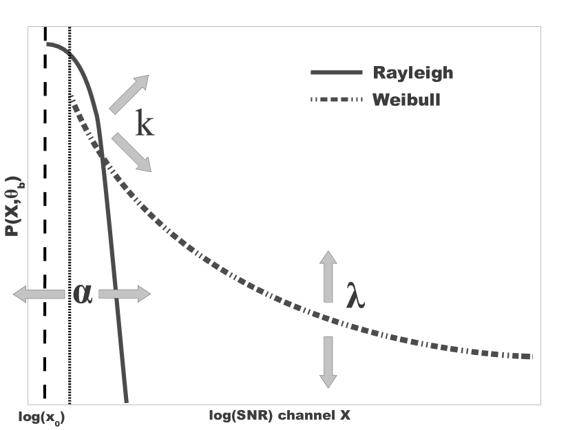
It is necessary to compute the discrete representation of in such a way as to best resolve all structure present. The histogram should have the most number of bins possible, without having an excessive number of near zero bin components. To construct such a histogram one needs to maximize the information entropy of the histogram [16]. The data sets contain a large range of observed SNRs, as such, it is better to discretize this data using logarithmically spaced bins, rather than linearly spaced ones. Consider a set of bin edges which are base logarithmically separated, the optimal choice of can be determined by maximizing the total histogram entropy. Selecting can be done iteratively, so that the resulting histogram of the data can easily be fit to the Rayleigh portion (low SNR) and also to the Weibull portion (high SNR) of . To properly fit this function the entropy of the histogram as a function of is computed. The value of is expected to be somewhere in the interval . One must also decide the number of bins that should be used for histogram construction. In order to determine the best binning to use one would simultaneously maximize the entropy of the histogram across both and . To discretely compute the entropy , requires computing the following quantity,
| (8) |
with the following normalization
| (9) |
The width scale of is logarithmically increasing by , and the value of is just the normalized element count in bin . Optimizing the logarithmic scaling to the highest bin resolution possible is simply a matter of identifying the global maximum of . The most accurate fit to the data is possible when using a histogram representation with the highest possible entropy.
It is important that sampled data set properly represent the underlying distributions, in order to create a proper fit for . Properly fitting the PDF involves determining the parameters, , , , , , while respecting the threshold . The choice of approach to determine the parameters is a direct consequence of the data set size, and ability to properly histogram the sampled data. Under typical circumstances, the approach of choice would be Quantile Maximum Product of Spacing (QMPS). In some cases the data sets are sparse. For this situation we use a fitting approach named Maximum Product of Spacing (MPS). The MPS approach uses all available data from the set and is inherently more tedious to apply than the QMPS approach. The two different approaches converge to the same parameters for data streams that are sufficiently sampled [17, 18].
The QMPS presented itself to be the most effective approach to determine the parameters of . The cumulative distribution function (CDF) of is defined from the CDF of
| (10) |
and from the CDF of
| (11) |
These two equations can be combined into the following form
| (12) |
The parameters of interest are found by maximizing the quantity using QMPS as follows,
| (13) | |||||
and all parameters can be fit simultaneously. Where is the element count for the bin. The parameter represents the left side bin value which comes from the maximum entropy histogram of data which should represent the distribution . Using this method will give us all the fitting parameters required to characterize the sampled data.
In the case that data samples are sparse, MPS is used to determine the parameters of interest. The MPS also seeks to maximize the quantity , but this approach varies as follows
| (14) | |||||
where is the total number of artifacts used to fit the parameters simultaneously. One should use QMPS whenever possible since implementing this calculation for very large becomes computationally costly.
5 Creating Coupled and Uncoupled Models
Artifacts used to construct the coupled model are selected by applying a time coincidence check, with a window of , which represents the largest absolute time difference between a GW channel artifact and sensor channel artifact. For this preliminary study we chose , after comparing a large collection of sensor data artifacts from many channels with GW data artifacts. When analyzing large sets of sensor channels, it is better to choose a value which is long enough to capture all artifacts resulting from control loop delays, and physical delays between an environmental effect and the expected GW detector response to this effect.
The coupled model data can be expressed as a conditional probability distribution (CPD) with the following form
| (15) |
where is a two dimensional joint probability distribution (JPD). This JPD represents the probability of a element in the set (GW data), given set (sensor data) for a specific model configuration . In this expression (foreground) denotes the set of coincident samples drawn during potential coupling times.
The data used to construct the uncoupled model is derived from all available and artifacts. Unlike the coupled model, the uncoupled model is intentionally designed to break the statistical relationship between the artifacts in and . Using the PDFs of and a background model JPD is built where we have forced statistical independence. This implies that the correct form for an uncoupled model’s JPD, is simply
| (16) |
where represents background samples used which are not members of the foreground set identified by the coupled model’s CPD, the discrete forms of and must be consistent with their counterparts contained in . In addition to knowing these functions one must also expect that the data which represents the coupling in the coupled model are not the dominate data source for constructing and This additional constraint is easily satisfied when building models between any one particular channel and the GW channel.
6 Calculation of CCL Function
The CCL function, introduced in equation 1, is the log likelihood ratio between the coupled and uncoupled models previously described, and should be expressed as follows:
| (17) |
The above expression is easy to simplify algebraically because of equation (16) yielding
| (18) |
The CCL function quantifies the level of suspected coupling between a specific sensor and the GW data. The observed CCL value can be translated into one of three statements: no coupling suspected; coupling suspected; or an indeterminate state with insufficient information to determine coupling. In the case of no coupling the CCL values will be negative indicating improbable coupling. For cases of coupling the CCL values will be positive indicating a potential GW channel candidate is likely due to a localized noise source influencing the GW detector. When the values are close to zero, either positive or negative, the test is incapable of determining whether the GW candidate is a noise artifact.
6.1 Visualizing and Interpreting CCL Functions
Visualizing a CCL function offers insight into the characteristics of the data. One can consider these functions as a two dimensional color map with the GW data, , plotted along the vertical axis and the sensor data, , plotted along the horizontal axis. When we plotted the preliminary functions we encountered distinct patterns in the CCL values as a function of SNR between the two data sets. One might expect there to be some sort of pattern visible in plots of CCL functions and these patterns tended to be distinct. The distinctness of these patterns is attributable to the coupling mechanism responsible. Upon reviewing many CCL plots, we noticed that they could be organized and characterized by specifically shaped regions of high significance artifacts. Figure 2 presents an illustrative cartoon superimposing several key regions observed from different sensor data onto one graph.
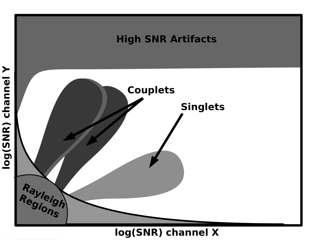
The color map, represents the CCL values calculated for the data set. All CCL functions will contain some part of or all of a triangular region we call Rayleigh Region, composed of three joined regions, one circular and two others triangular in shape (figure 2). The artifacts appearing in this region must be assumed to be related to Gaussian fluctuations in either the sensor or the GW channels. There is no way to distinguish Rayleigh artifacts, which are not coupled, from potentially coupled artifacts, which lay in one of the two smaller triangular regions. Artifacts in these two smaller regions are the product of convolutions of inherent Rayleigh noise with potentially interesting Weibull noise components. This convolution results in having only one of two pieces of useful information needed to identify coupling. For these two triangular regions CCL values here are typically near zero. This is different from the shaded circular region in figure 2 whose artifacts are composed from two pieces of inherent noise which is Rayleigh distributed. For real data shown later, this shaded circular region can be less pronounced but is located in approximately the same region of the plot. In this case CCL values may take on a larger range of negative values. The three Rayleigh related regions are inherent to all CCL functions and typically present in some form.
The next region of interest is the Singlet region. Here the CCL values show what appears to be a quasi-linear relationship in a log-log space of observed artifact’s SNR in the sensor data compared with the artifacts in the GW data. Another region of interest is Couplets and this structure is normally seen in pairs of CCL functions. Consider two sensor channels that measure similar but not identical physical phenomena like ground motion, which can affect accelerometers and seismometers. Excessive ground motion at the detector might produce similarly distributed artifacts in both channels and the corresponding CCL function plots can share similar structures which appear like adjacent or overlapping singlets. The last region observed in most CCL functions, which is not sharply defined, is the High SNR Artifacts region. The events that compose this region are at the edge of linear behavior for differential arm motion sensing. Because of the potential for a non-linear instrument response, this region presents itself as unreliable [19]. These plots are useful as supplementary tools to visualize and help understand the relationships between the sensors and the detector output.
6.2 Disregarding CCL functions sensitive to gravitational waves
The detector should in principle have its output, the GW data, as the only data stream which is sensitive to GWs. In practice this is not guaranteed to be the case. The detector may have sensors which react to the presence of a GW. It is unwise and not safe to use a CCL function derived from sensors which may be responding to passing GWs. One needs a prescription for identifying sensor channels that are unsafe so those functions will not be used to identify non-GW artifacts in the detector output [20].
An unsafe CCL function, with possible undesirable sensitivity to GW phenomena, can be identified with a simple prescription. If the CCL function is unsafe, then the distribution of hardware injections identified by an individual CCL function will be similar to the distribution of all artifacts due to hardware injections used to test the detector. Hardware injections are control signals introduced in the detector which simulate its physical response to GW signals. It is the resulting response what is recorded in the GW channel [21]. Using these injections it should be straightforward to identify unsafe CCL functions. This identification process is accomplished by using a Kolmogorov-Smirnov (KS) test. The null hypothesis would be, “For a given sensor , is the distribution of the hardware injection artifacts, identified with the same as the distribution of all known hardware injection artifacts?”. A CCL function is tested for safety using
| (19) |
with
| (20) |
where represents an SNR threshold, represents the set of all hardware injection artifacts identified with and are all known hardware injection artifacts. In applying our KS test, for a given significance level() one would accept or reject the specified null hypothesis [22]. If the left hand side (LHS) of equation 19 exceeds the chosen then one should accept the null hypothesis because the artifact identified by the CCL function are being preferentially selected from set of all known hardware injections. Acceptance of the null hypothesis means that the sensor channel is unsafe. In the case that the LHS of equation 19 doesn’t exceed , the sensor channel used to construct the CCL function is safe. This preliminary study required the boundary between safe and unsafe to be set by , which means that at the confidence level we are sure of the safety or lack of safety for a tested sensor channel. This method of safety testing determined which sensor channels are safe and suitable for analysis with the CCL method.
7 Preliminary Results
We will show how the Critical Coupling Likelihood (CCL) method responds to artifacts in LIGO data, while ignoring effects that can be attributed to potential GW signals. The data used in this analysis is a set of sampled instrument times, which were pre-processed with a TF transformation tool called the omega pipeline. This tool was chosen primarily because this transformation used a wavelet decomposition basis which worked well for resolving signals with low frequency components [23]. The total aggregate time of our data samples is equivalent of 3.5 days of observing data, derived from sampling two months near the end of S6 for LIGO Livingston and LIGO Hanford observatories.
The costs of using CCL in the future are dependent on many factors. The most costly phase of a CCL end to end analysis is the data pre-processing step. In order to apply CCL to an online detector one would need at least 1 compute core per every 5 to 10 sensor channels being analyzed. This estimate is reasonable if one assumes getting the sensor data to the compute core is instantaneous. The actual computational costs of the CCL method could be much higher depending on implementation of CCL, the pre-processor and data handling at each detector site.
The results presented here are intended to motivate the development of the CCL method, highlight typical CCL functions, and show encouraging results derived from a limited set of input sensors. The reader should bear in mind that these results are from a single case study using CCL. There still remains a great deal of optimization, use of higher dimensional approaches (use of more artifact properties) and studies with larger sets and fine tuning also can be performed.
The goal of a CCL analysis is to make quantitative statements about the instrument behavior relative to the studied sensor data. The CCL output is a single quantitative value, per available sensor data set, which is useful to determine the coupling state of the detector. The CCL functions have behaved differently when applied to LIGO Livingston in comparison with LIGO Hanford. This difference in behavior is unremarkable and likely attributable to the distinctly different operating environments.
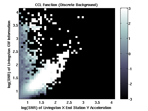
As an example LIGO Livingston is plotted in figure 3a. The identifiable structure in this plot is an example of a Singlet. The singlet in this function is indicative of coupling to the instrument through seismic motion. The seismic motion induces an acceleration of an accelerometer mounted on an optics table in close proximity to one of LIGO’s large optics(test mass). This optic is pitching back and forth while suspended at the end of one of LIGO’s two arms as a result of optical table motion. The optics increasing motion corresponds with increasing SNR of artifacts in the GW detector output. This relationship is readily seen in the figure as an angled structure of high CCL values.
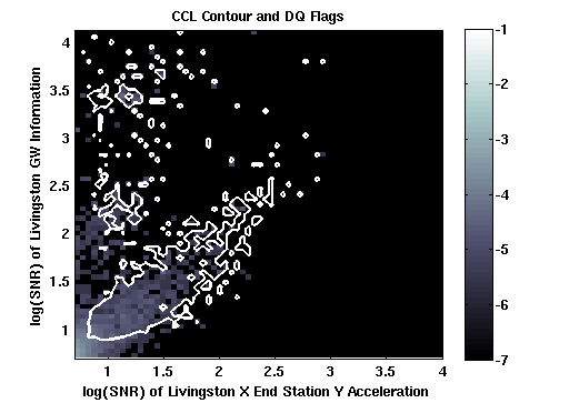
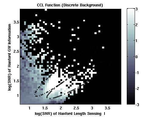
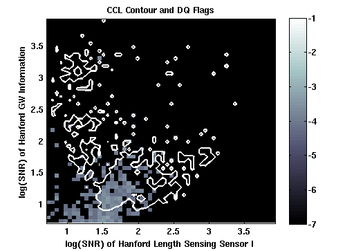
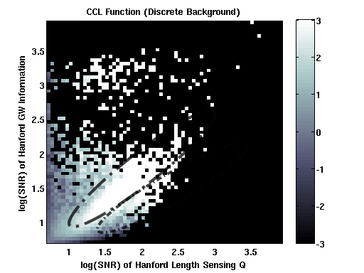
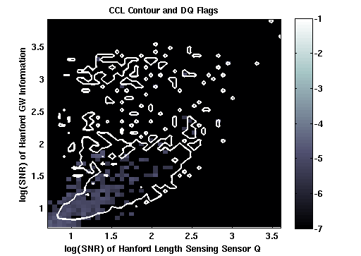
Another type of CCL structure example is shown using LIGO Hanford data in figures 4a and 5a. These figures shows a different type of identifiable structure, a “Couplet”. For CCL functions with this type of structure, the artifacts identified by this model can typically be associated with another sensor. In both figures, there appears to be two angled structures, not always easily distinguishable, but in this case one structure is better defined than the other. In figure 4a, the well defined angled structure(short dashes) corresponds to a poorly defined, but similar structure in figure 5a. This relationship is reciprocal, the well defined angled structure(long dashes) associated with figure 5a is the poorly defined structure associated with the couplet from figure 4a. The couplet structure appears in pairs of CCL functions. These pairs are usually related by obvious mechanisms as in demodulated signals or signals derived from mechanically interdependent systems. For these example figures, the two data channels are registering artifacts which have both in-phase and quadrature components of light received by the same photo-diode assembly. The in-phase component of light tracks common motion of the input optics which form the long Fabry-Perot arms of the interferometer. The quadrature phase tracks the differential motion of the input optic of the cavity. Laser power fluctuations can induce optic motion impacting the length of the Fabry-Perot cavities. These length changes can take the cavity off resonance and allow energy to exit the cavity. The energy exiting the cavity can transfer power from one arm to another leading to differential motion of the input optics. These two types of motion, common and differential, can excite one another and make controlling the full length interferometer difficult thereby increasing the noise in the interferometer.
The CCL method can provide a quantified measure describing coupling into the detector data. This measure is useful to understand if and what local environmental effects may be responsible for a false GW event. To appreciate the potential usefulness of a method like the CCL, we imposed a CCL threshold value. Thus exceeding this value declares an event as noise coupled to the detector. By using a CCL cutoff, , it allows us to sort the identified artifacts into two groups: inherent noise artifacts (uncoupled) and those which are due to environmental effects (coupled). This CCL value corresponds to an identified artifact is at least times more likely to be coupled than uncoupled, as defined in section 6.
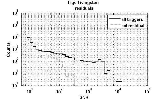
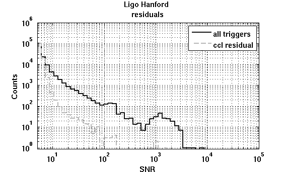
For LIGO Livingston, a total of 205 functions were used to identify the coupled artifacts. For LIGO Hanford, we used a total of 207 functions to identify the coupled artifacts in the Hanford data set. The set of artifacts analyzed were constructed by sampling Livingston and Hanford data with an average sampling rate of 1 sample, which is 1 second in duration, every two minutes using only science mode times. Science mode times are periods where the instrument is operating at the minimum level of data quality that should be considered viable to perform a search for GW signals [5]. Using this sampling constraint, the data set is less than of the total amount of data available from two months near the end of LIGO’s sixth science run. We expect that if more samples were taken during the same interval of observation time the results of our preliminary analysis will remain relatively unchanged. Using these constraints on sampling rate and sensors used, figures 6 and 7 show the number of artifacts not identified as coupled after applying a CCL cut. For both figures, there is a clear suppression of the original outlier tails. What may not be readily apparent in these figures is that the CCL method appears able to suppress the outlier tail and identify moderate SNR artifacts, while leaving the original low SNR artifact distribution unchanged. In table 1, it is easier to see why one can appreciate the CCL method for identifying artifacts, because this method ignores SNR regions where artifacts tend to be the result of inherent noise properties of the instrument. This suppression of the outlier tail in this study is accompanied by a data volume cost. The amount of gravitational wave data that should be discarded, at least for this single case, is moderately high at and of the tested data for LIGO Livingston and LIGO Hanford respectively. A LIGO type detector has noise sources which are clearly non-Gaussian in nature. Some of these excesses have been identified, and are more pronounced in LIGO’s low frequency bands of , which is thought to account for on order of , of the excess outlier tail [9]. The artifacts contributing to the discarded data show a clear selection of non-Gaussian type artifacts. It is likely that our observed discarded data volume is not the result of our analysis configuration, but may actually be the product of an epoch which is less well behaved than one might expect. Further studies using CCL are called for but with this single case study there is already evidence that this method may prove to be beneficial for GW searches.
| Livingston | Hanford | |
|---|---|---|
| Deadtime | 13.9% | 15.1% |
| SNR() | % | % |
| 5 | 14.4 | 16.3 |
| 8 | 82.3 | 93.5 |
| 10 | 88.8 | 96.7 |
| 20 | 86.7 | 98.0 |
| 50 | 92.4 | 98.9 |
| 100 | 98.0 | 99.2 |
The sensor channels used in this preliminary study were those of the standard follow-up activities done at the end of a GW search [7, 8]. Using the safety prescription outlined in section 6.2 we discarded several channels presenting undesirable sensitivity to GW phenomena and considered them potentially unsafe. According to our chosen criteria, we were required to remove 10 channels for LIGO Hanford, and 9 channels for LIGO Livingston. Of the channels removed, a large fraction were consistent with channels suspected to be unsafe, with a few exceptions. One example unsafe channel noted for both detectors was the channel which records the amount of light incident on the detector’s output mode cleaner. The light that is incident on the mode cleaner should contain the signature of a passing GW so, it would be unwise to use this channel as an indicator of detector noise. Not all channels failing to meet the safety criteria were common to both detectors. In general the types of channels that were consistently seen as unsafe, were either related to the output of the detector, or part of the feedback control of the detector.
One can see in table 2, that the remaining safe channels identify a small fraction of the total number of hardware injection artifacts. There is a notable contrast between the safe and unsafe functions, because as one can see from tables 2 and 3 the median number of hardware injections identified per CCL function for safe channels is lower than those for unsafe channels.
| Safe CCL Function Properties | ||
|---|---|---|
| Livingston | Hanford | |
| Median Injection Count Per Channel | 2 | 4 |
| Mean Injection Count Per Channel | 2.7(1.04%) | 4.7(1.54%) |
| Standard Deviation on Count Per Channel | 2.3(0.87%) | 4.2(1.39%) |
| Hardware injection artifacts in data set | 265 | 303 |
| Total Number of Channels | 205 | 207 |
| Unsafe CCL Function Properties | ||
|---|---|---|
| Livingston | Hanford | |
| Median Injection Count Per Channel | 7 | 9 |
| Mean Injection Count Per Channel | 6.8(2.58%) | 9.2(3.04%) |
| Standard Deviation on Count Per Channel | 1.2(0.47%) | 3.1(1.05%) |
| Hardware injection artifacts in data set | 265 | 303 |
| Total Number of Channels | 9 | 10 |
| Ph.D. Thesis, MIT Dept. of Physics | ||
8 Conclusions and Future Directions
The Critical Coupling Likelihood method is intended to improve future GW search efficiency and provide feedback to instrument scientists at the observatory. The results shown here are preliminary and are produced using a small set of LIGO data. The results shown use only the simplest form of CCL functions, capitalizing on the properties SNR and coincidence. We expect to see this same level of performance if we apply this approach to a full set of existing LIGO data or future aLIGO data. This method is promising because it offers quantified detector information which can be directly imported into a GW search. In creating this quantified detector information, the CCL method is also providing instrument scientists with information that describes potential coupling mechanisms between the instruments operating environment and behavior. We plan to present the instrumental implications of the CCL method in a later paper.
In this paper we introduced a new detector characterization technique called the CCL method. This method is intended to use all available observatory information and deduce the presence of coupling between the environment and the detector. In making this coupling identification it also implicitly estimates the coupling relationship giving information about how the strength of local environmental effects map into specific noise levels and frequency bands. These preliminary results indicate that an approach like CCL should have an appreciable impact on the effectiveness of future GW searches, by reducing the outlier tail. Our initial results show CCL identifying of observed artifacts with . Identifying these outlier events leads to significant outlier tail suppression which is clearly seen in figures 6 and 7. By using this technique we can quantitatively characterize individual GW candidates, accounting for instrumental conditions, and hence improve GW searches and the validation of a detection.
9 Acknowledgments
The authors gratefully acknowledge the support of the United States National Science Foundation for the construction and operation of the LIGO Laboratory. The authors also thank LIGO and the LIGO Scientific Collaboration for allowing the use of LIGO data for this study. The authors would also like to acknowledge the support of this research via NSF grants PHY-0905184 and PHY-0757058. C Costa also thanks to CNPq 300001/2012-6 by financial support. This paper was assigned LIGO document number LIGO-P1000187.
References
References
- [1] http://www.ligo.org
- [2] Harry G et al 2010 Class. Quantum Grav. 27 084006
- [3] Abadie J et al 2010 Class. Quantum Grav. 27 173001
- [4] Mandel I et al 2008 ApJ 681 1431
- [5] Abbott B et al 2007 Class. Quantum Grav. 24 5343
- [6] Slutsky J et al 2010 Class. Quantum Grav. 27 165023
- [7] Torres C and Gouaty R 2010 The Compact Binary Coalescence Search Follow-up the “Home Stretch” International School on Numerical Relativity and Gravitational Waves Asia Pacific Center for Theoretical Physics, Pohang Korea LIGO-G1000679
- [8] Gouaty R 2008 Class. Quantum Grav. 25 184006
- [9] Abbott B et al 2009 Phys. Rev. D, 79, 122001
-
[10]
LIGO Scientific Collaboration and Virgo Collaboration, 2011
https://dcc.ligo.org/public/0062/T1100322/003/PublicWhitePaper.pdf - [11] Abbott B et al 2004 LIGO Scientific Collaboration Phys Rev.D 69 122004
- [12] McDonough R and Whalen A 1995 Detection of Signals in Noise Academic Press
- [13] Christensen N et al 2010 Class. Quantum Grav., 27, 194010
- [14] Nelson W 2003 Applied Life Data Analysis Wiley-Interscience
- [15] Hernandez J and Phillips I 2006 IEE Proc. Commun. 153, 2
- [16] Collins R and Wragg A 1977 J. Phys. A:Math. Gen., Vol. 10 No. 9
- [17] Cheng R and Amin N 1983 J. R. Stat. Soc. Ser. B Stat. Methodol. 45(3) 394
- [18] Cousineau D 2009 IEEE Trans. on Dielect. and Elect. Ins. 16(1) 281
- [19] Abadie J et al 2010 NUCL INSTRUM METH A 624 223
- [20] Leroy N et al 2009 Class. Quantum Grav. 26 204007
- [21] Brown D 2004 Class. Quantum Grav. 21 S797-S800
- [22] Sheskin D 2007 Handbook of parametric and nonparametric statistical procedures 4th ed Chapman and Hall
- [23] Chatterji S 2005 The search for gravitational wave bursts in data from the second LIGO science run PhD Thesis Massachusetts Institute of Technology