Abstract

The energy level density distributions of some Haldane-Shastry like spin chains associated with the $A_{N-1}$ root system have been computed recently by Enciso et al., exploiting the connection of these spin systems with inhomogeneous one-dimensional vertex models whose energy functions depend on the vertices through specific polynomials of first or second degree. Here we consider a much broader class of one-dimensional vertex models whose energy functions depend on the vertices through arbitrary polynomials of any possible degree. We estimate the order of mean and variance for such energy functions and show that the level density distribution of all vertex models belonging to this class asymptotically follow the Gaussian pattern for large number of vertices. We also present some numerical evidence in support of this analytical result.

PACS No.: 02.30.Ik, 75.10.Jm, 05.30.-d

Keywords: Haldane-Shastry spin chain, vertex model, Yangian quantum group, level density distribution

1 Introduction

As is well known, one-dimensional (1D) quantum integrable spin chains can be broadly classified into two types depending on their range of interaction. One such class consists of spin chains having only local interactions like nearest or next-to-nearest neighbour interaction. Isotropic and anisotropic versions of Heisenberg spin-$\frac{1}{2}$ chain, Hubbard model etc. are examples of this type of spin models with short range interaction [1, 2, 3]. However, there exist another class of 1D quantum integrable spin systems for which all constituent spins mutually interact with each other through long range forces [1, 4]. Haldane-Shastry (HS) spin chain [5, 6], Polychronakos spin chain (also known as Polychronakos-Frahm (PF) spin chain) [7, 8, 9] and Frahm-Inozemstsev (FI) spin chain chain [10, 11] are well known examples of quantum integrable spin systems with long range interaction. This type of spin chains have attracted a lot of attention in recent years due to their exact solvability and applicability in a wide range of subjects like generalized exclusion statistics and fractional quantum Hall effect [12, 13, 14, 15], SUSY Yang-Mills theory and string theory [16, 17, 18, 19, 20], Yangian quantum group [21, 22, 23, 24, 25, 26, 27, 28] etc. For the simplest case of $A_{N-1}$ root system, the Hamiltonians of $su(m)$ invariant, ferromagnetic type HS, PF and FI spin chains can be written in a general form like [4, 5, 6, 7, 8, 9, 10, 11]

$${H}~{}=~{}\sum_{1\leq j<k\leq N}~{}\frac{1-P_{jk}}{f(\xi_{j}-\xi_{k})}\,.$$ (1.1)

Here $\xi_{j}$ denotes the position of the $j$-th lattice site, spins can take $m$ possible values on each lattice site, ${P}_{jk}$ represents the exchange operator which interchanges the spins on the $j$-th and $k$-th lattice sites and the strength of this exchange interaction is determined by the function $f(\xi_{j}-\xi_{k})$. It should be noted that, while the lattice sites of HS spin chain are uniformly distributed on a circle, the lattice sites of PF and FI spin chain are non-uniformly distributed on a straight line. Supersymmetric generalizations of the spin chains (1.1) have also been studied in the literature [13, 29, 30, 31].

The difference between quantum integrable models with short range interaction and long range interaction manifests very prominently through their connection with classical vertex models. It is well known that the Hamiltonians of 1D quantum integrable spin chains with short range interaction are related to the transfer matrices of some exactly solvable 2D vertex models in statistical mechanics [32, 33]. However, there exists no simple relation between the energy levels of such 1D spin chains and the energy functions of corresponding 2D vertex models. On the other hand, a direct connection between the energy levels of 1D quantum integrable spin chains with long range interaction and energy functions of 1D vertex models can be inferred from some works in the literature [24, 26, 34]. Indeed, by applying a rather general technique based on Yangian quantum group symmetry, it has been shown recently that the energy levels for a class of HS like spin chains as well as their supersymmetric generalizations exactly coincide with the energy functions of some 1D inhomogeneous vertex models in classical statistical mechanics [35].

The reason behind the close connection between 1D quantum spin chains with long range interaction and 1D classical vertex models can be traced from the underlying Yangian quantum group symmetry of the spin Hamiltonians, which allows one to write down their exact spectra in closed forms even for finite number of lattice sites. In the following, we shall briefly recapitulate the consequences of Yangian symmetry for the special case of nonsupersymmetric $su(m)$ ferromagnetic spin chains. A class of irreducible representations of the $Y(sl_{m})$ Yangian algebra, known as ‘border strips’ or ‘motifs’, completely span the Hilbert space of some Yangian invariant spin systems with long range interaction [13, 4, 21, 22, 23, 24, 25, 26, 27, 28]. For the case of a spin system with $N$ number of lattice sites, boarder strips are denoted by $\langle k_{1},k_{2},\ldots,k_{r}\rangle$, where $k_{i}$’s can be taken as any positive integers satisfying the relation $\sum_{i=1}^{r}k_{i}=N$. Thus the Hilbert space associated with a Yangian invariant spin system may be decomposed as

$$\mathcal{V}=\sum\limits_{k_{1}+k_{2}+\ldots+k_{r}=N}\oplus\hskip 5.69046pt{V}_{\langle k_{1},k_{2},\ldots,k_{r}\rangle}\,,$$ (1.2)

where ${V}_{\langle k_{1},k_{2},\ldots,k_{r}\rangle}$ denotes the irreducible vector space associated with boarder strip $\langle k_{1},k_{2},\ldots,k_{r}\rangle$. Let us restrict our attention to a class of Yangian invariant spin systems, for which the complete set of energy levels can be written in the following way:

$$E_{\langle k_{1},k_{2},\ldots,k_{r}\rangle}=\sum_{l=1}^{r-1}\mathcal{E}_{N}(j)|_{j=K_{l}}\,,$$ (1.3)

where $K_{l}=\sum_{i=1}^{l}k_{i}$, and $\mathcal{E}_{N}(j)$ is an arbitrary function of the discrete variables $j$ and $N$. Due to Yangian symmetry of this class of spin systems, the multiplicity of the eigenvalue $E_{\langle k_{1},k_{2},\ldots,k_{r}\rangle}$ in Eq. (1.3) coincides with the dimensionality of the vector space ${V}_{\langle k_{1},k_{2},\ldots,k_{r}\rangle}$. Hence, this type of energy eigenvalues are highly degenerate in general. It should be noted that, all energy levels of $su(m)$ ferromagnetic HS, PF and FI spin chains can be generated through Eq. (1.3) as special cases, where $\mathcal{E}_{N}(j)$’s are given by ‘dispersion relations’ of the form [21, 22, 23, 24, 25, 26, 27, 28, 34]

$$\mathcal{E}_{N}(j)=\left\{\begin{array}[]{ll}j(N-j),&\mbox{for the HS chain}\\ j,&\mbox{for the PF chain}\\ j(c+j-1),~{}\mbox{with}~{}c>0,&\mbox{for the FI chain.}\end{array}\right.$$ (1.4)

The spectra of all Yangian invariant spin chains associated with Eq. (1.3) can be written in an elegant alternative form by using the energy functions of corresponding 1D inhomogeneous vertex models [35]. Let us consider a class of 1D classical vertex models with $(N+1)$ number of vertices, which are connected through $N$ number of intermediate bonds. Each of these bonds can take one of the $m$ possible states. Therefore, any state for such vertex models can be represented by a path configuration of finite length:

$$\vec{s}\equiv\{s_{1},s_{2},\ldots,s_{N}\},$$ (1.5)

where $s_{i}\in\{1,2,\cdots,m\}$ denotes the spin state of the $i$-th bond. For constructing vertex models corresponding to Yangian invariant spin chains whose energy levels are given by Eq. (1.3), let us define an ‘energy function’ related to the spin path configuration $\vec{s}$ as

$$E(\vec{s})=\sum_{j=1}^{N-1}\mathcal{E}_{N}(j)\delta(s_{j},s_{j+1}),$$ (1.6)

where $\delta(s_{j},s_{j+1})$ is taken as

$$\delta(s_{j},s_{j+1})=\left\{\begin{array}[]{rl}0&\text{if}\hskip 5.69046pts_{j+1}\leq s_{j}\\ 1&\text{if}\hskip 5.69046pts_{j+1}>s_{j}\,.\end{array}\right.$$ (1.7)

It should be noted that, the same function $\mathcal{E}_{N}(j)$ has appeared in Eqs. (1.6) and (1.3). It can be shown that, for all possible functional forms of such $\mathcal{E}_{N}(j)$, the spectrum of the $su(m)$ ferromagnetic spin chain generated by eigenvalues (1.3) (along with the degeneracy factors of these energy levels) completely matches with that of the corresponding vertex model generated by energy functions (1.6) [35]. In particular, the full spectra of $su(m)$ ferromagnetic HS, PF and FI spin chains can be reproduced from the energy function (1.6), by substituting to it the corresponding forms of dispersion relations given in Eq. (1.4). Hence, it is possible to extract important informations about the statistical properties of the spectra of these spin chains by analyzing the distribution of energy functions for the related 1D vertex models. With the help of numerical studies, it has been conjectured for a long time that the energy level densities for this type of spin chains asymptotically follow the Gaussian distribution as the number of lattice sites become very large [36, 37, 38, 39, 40, 41, 11]. By using the above mentioned connection with 1D vertex models, very recently this conjecture has been proved analytically for the case of $su(m)$ HS, PF and FI spin chains associated with the $A_{N-1}$ root system [34].

In this context, it is interesting to ask whether the Gaussian level density distribution of HS, PF and FI spin chains is simply a consequence of their Yangian quantum group symmetry or this result crucially depends on the specific forms of the dispersion relations given in Eq. (1.4). To answer this question, in this article our aim is to explore the level density distribution of the energy function (1.6) for a large class of 1D vertex models, for which $\mathcal{E}_{N}(j)$ can be chosen as an arbitrary polynomial of the variables $j$ and $N$. Even though it may not be possible in general to express the Hamiltonians of the spin chains corresponding to such vertex models in a simple form like (1.1), one can formally express those Hamiltonians in dyadic notation through the basis vectors of the Hilbert space $\mathcal{V}$ in the following way. Let us denote the basis vectors of the subspace ${V}_{\langle k_{1},k_{2},\ldots,k_{r}\rangle}$ in Eq. (1.2) with the notation $|\psi_{k_{1},k_{2},\ldots,k_{r};{\bf{\alpha}}}\rangle$, where ${\bf{\alpha}}\in\{1,2,\cdots,\bf{\rho_{k}}\}$, and $\bf{\rho_{k}}$ is the dimension of ${V}_{\langle k_{1},k_{2},\ldots,k_{r}\rangle}$. The Hamiltonians for the above mentioned class of Yangian invariant spin chains may now be written as

$$\mathcal{H}=\sum\limits_{k_{1}+k_{2}+\ldots+k_{r}=N}\hskip 2.84544pt\hskip 2.84544ptE_{\langle k_{1},k_{2},\ldots,k_{r}\rangle}\sum_{{\bf{\alpha}}=1}^{\bf{\rho_{k}}}|\psi_{k_{1},k_{2},\ldots,k_{r};{\bf{\alpha}}}\rangle\langle\psi_{k_{1},k_{2},\ldots,k_{r};{\bf{\alpha}}}|\,,$$ (1.8)

where $E_{\langle k_{1},k_{2},\ldots,k_{r}\rangle}$ is given by Eq. (1.3), with $\mathcal{E}_{N}(j)$ being an arbitrary polynomial function of $j$ and $N$. Hence, in the following, our aim is also to explore the level density distribution for the class of spin chains represented by $\mathcal{H}$ in Eq. (1.8).

The arrangement of this article is as follows. In Sec.2 we briefly recapitulate the transfer matrix approach of Ref.[34], where it has been found that the level densities for the case of nonsupersymmetric HS, PF and FI spin chains and related 1D vertex models asymptotically follow the Gaussian distribution as the size of these systems become very large. In Sec.3 we show that the above mentioned approach can be applied to analytically compute the level density distribution for a wide range of 1D vertex models and related spin chains, for which the dispersion relations are taken as arbitrary polynomials of the variables $j$ and $N$. In this section, we also find out the order of mean and variance for the energy functions or energy levels associated with such dispersion relations. In Sec.4 we numerically study the level density distribution for some 1D vertex models with different choice of the related parameters and find that these numerical results are in complete agreement with the analytical prediction of the previous section. In Sec.5 we summarize our results and make some concluding remarks on the possible connection between Yangian quantum group symmetry of a spin chain and the asymptotic form of its level density distribution.

2 Level density for known HS like spin chains

In this section, we review the transfer matrix approach for calculating the level density distributions in the cases of ferromagnetic $su(m)$ HS, PF and FI spin chains related to the $A_{N-1}$ root system [34]. A key role in this approach is played by the normalised characteristic function of the level density distribution. Utilizing the equivalence of these spin chains with 1D vertex models, such normalised characteristic function may be defined as

$$\hat{\phi}_{N}(t)=\langle e^{\frac{it(E(\vec{s})-\mu)}{\sigma}}\rangle\,,$$ (2.1)

where $E(\vec{s})$ is the energy function (1.6) of the vertex model associated with the spin chain, $\mu$ and $\sigma$ denote the mean and the variance of this energy function respectively, and the notation $\langle\mathcal{O}\rangle$ represents the average of $\mathcal{O}$ over all spin path configurations. If this characteristic function satisfies the asymptotic relation

$$\lim_{N\rightarrow\infty}\hat{\phi}_{N}(t)=e^{-\frac{t^{2}}{2}}\,,$$ (2.2)

then it can be shown that [42] at $N\rightarrow\infty$ limit the normalised level density approaches to a Gaussian distribution of the form

$$G(E)=\frac{1}{\sqrt{2\pi\sigma^{2}}}e^{-\frac{(E-\mu)^{2}}{2\sigma^{2}}}.$$ (2.3)

Therefore, instead of directly working with the level density of a spin chain, one can study the $N\rightarrow\infty$ limit of the related characteristic function. Inserting the form of $E(\vec{s})$ given in Eq. (1.6) to Eq. (2.1), it is easy to express $\hat{\phi}_{N}(t)$ as

$$\hat{\phi}_{N}(t)=m^{-N}e^{-\frac{i\mu t}{\sigma}}Z_{N}(e^{\frac{it}{\sigma}})\,,$$ (2.4)

where the ‘partition function’ $Z_{N}(e^{\frac{it}{\sigma}})$ is defined through a product of transfer matrices as

$$Z_{N}(e^{\frac{it}{\sigma}})=m^{N-1}\sum_{n,n^{\prime}=1}^{m}\big{[}T(\omega_{1})T(\omega_{2})\ldots T(\omega_{N-1})\big{]}_{nn^{\prime}}\,.$$ (2.5)

Here the transfer matrix $T(\omega_{j})$ is given by $T(\omega_{j})=T(\omega)|_{\omega=\omega_{j}}$, with

$$T(\omega)=\frac{1}{m}\begin{pmatrix}1&\omega^{m}&\cdots&\omega^{m}\\ \vdots&\ddots&\ddots&\vdots\\ \vdots&&\ddots&\omega^{m}\\ 1&\ldots&\ldots&1\end{pmatrix}\,,$$ (2.6)

$\omega_{j}=e^{i\gamma_{j}t}$ and

$$\gamma_{j}=\frac{\mathcal{E}_{N}(j)}{m\sigma}.$$ (2.7)

Since this transfer matrix can be diagonalised through an unitary transformation, it may be written as

$$T(\omega_{j})=U(\omega_{j})D(\omega_{j})U^{\dagger}(\omega_{j}),$$ (2.8)

where $U(\omega_{j})$ is an unitary matrix with elements given by

$$U_{nn^{\prime}}(\omega_{j})=\frac{1}{\sqrt{m}}\,\big{(}\omega_{j}e^{\frac{2\pi in^{\prime}}{m}}\big{)}^{m-n},$$ (2.9)

and $D(\omega_{j})$ is a diagonal matrix:

$$D(\omega_{j})=\text{diag}\hskip 2.84544pt\big{(}\lambda_{1}(\omega_{j}),\ldots,\lambda_{m}(\omega_{j})\big{)}\,,$$ (2.10)

with

$$\lambda_{k}(\omega_{j})=\frac{1}{m}\sum_{r=0}^{m-1}\left(\omega_{j}e^{\frac{2\pi ik}{m}}\right)^{r}\,.$$ (2.11)

With the help of Eqs. (2.4), (2.5) and (2.8), one can express $\hat{\phi}_{N}(t)$ as

$$\hat{\phi}_{N}(t)=\frac{e^{-i\mu t/{\sigma}}}{m}\sum_{n,n^{\prime}=1}^{m}M_{nn^{\prime}}(t),$$ (2.12)

where the matrix $M$ is given by

$$M(t)=U\left(\omega_{1}\right)D\left(\omega_{1}\right)B_{1}(t)\cdots D\left(\omega_{N-2}\right)B_{N-2}(t)D\left(\omega_{N-1}\right)U^{\dagger}\left(\omega_{N-1}\right),$$ (2.13)

with

$$B_{j}(t)=U^{\dagger}\left(\omega_{j}\right)U\left(\omega_{j+1}\right).$$ (2.14)

It should be observed that, Eq. (2.12) is derived without assuming any specific form of the dispersion relation. Furthermore, for any functional form of $\mathcal{E}_{N}(j)$, the mean and the variance of the energy function $E(\vec{s})$ in Eq. (1.6) can be expressed as [34]

$$\mu\equiv\langle E(\vec{s})\rangle=\frac{1}{2}\bigg{(}1-\frac{1}{m}\bigg{)}\sum_{j=1}^{N-1}\mathcal{E}_{N}(j),$$ (2.15)

and

$$\sigma^{2}\equiv\langle\left(E(\vec{s})-\mu\right)^{2}\rangle=\bigg{(}1-\frac{1}{m^{2}}\bigg{)}\bigg{[}\frac{1}{4}\sum_{j=1}^{N-1}\mathcal{E}_{N}(j)^{2}-\frac{1}{6}\sum_{j=1}^{N-2}\mathcal{E}_{N}(j)\mathcal{E}_{N}(j+1)\bigg{]}.$$ (2.16)

However, for determining the $N\rightarrow\infty$ limit of $\hat{\phi}_{N}(t)$ in Eq. (2.12), it is necessary to choose some specific form of the dispersion relation. Inserting the specific forms of dispersion relations given in Eq. (1.4) to Eqs. (2.15) and (2.16), one can explicitly obtain $\mu$ and $\sigma^{2}$ (as some functions of $m$ and $N$) for the cases of HS, PF and FI spin chains. By plugging such explicit forms of $\sigma$ in Eq. (2.7), it can be shown that the asymptotic behaviours of $\gamma_{j}$ and $\gamma_{j}-\gamma_{j+1}$ for large values of $N$ are given by the following relations in the cases of all these three spin chains [34]:

$$\gamma_{j}=O(N^{-1/2})\,,$$ (2.17)

and

$$\gamma_{j}-\gamma_{j+1}=O(N^{-3/2})\,,$$ (2.18)

where $j\in\{1,2,\ldots,N-1\}$ and the notation $f(N)=O(N^{a})$ implies that

$$\lim\limits_{N\rightarrow\infty}|N^{-a}f(N)|=\tau\,,$$ (2.19)

with $\tau$ being some non-negative real number. With the help of Eqs. (2.9) and (2.17), it is easy to show that

$$U\left(\omega_{j}\right)=R+O(N^{-1/2})\,,$$ (2.20)

where $R$ is a constant unitary matrix with elements given by

$$R_{nn^{\prime}}=\frac{1}{\sqrt{m}}e^{-2\pi inn^{\prime}/m}\,.$$ (2.21)

By using Eqs. (2.9), (2.14) and (2.18), one can also determine the asymptotic form of $B_{j}(t)$ as

$$B_{j}(t)=1\hskip-2.84526pt{\rm l}+O(N^{-3/2}).$$ (2.22)

Substituting the relations (2.20) and (2.22) to Eq. (2.13) and taking the $N\rightarrow\infty$ limit, one obtains

$$\lim_{N\rightarrow\infty}M(t)=R\Lambda(t)R^{\dagger},$$ (2.23)

where $\Lambda(t)$ is a diagonal matrix given by

$$\Lambda(t)=\text{diag}\hskip 2.84544pt\big{(}\Lambda_{1}(t),\ldots,\Lambda_{m}(t)\big{)}\,,$$ (2.24)

with

$$\Lambda_{k}(t)=\lim_{N\rightarrow\infty}\prod_{j=1}^{N-1}\lambda_{k}(\omega_{j})\,.$$ (2.25)

Taking the $N\rightarrow\infty$ limit of Eq. (2.12), and subsequently using Eqs. (2.23), (2.21) and (2.25), it is easy to find that

$$\lim_{N\rightarrow\infty}\hat{\phi}_{N}(t)=e^{-\frac{it\mu}{\sigma}}\Lambda_{m}(t)=e^{-\frac{it\mu}{\sigma}}\lim_{N\rightarrow\infty}\prod_{j=1}^{N-1}\lambda_{m}(\omega_{j})\,.$$ (2.26)

By putting $k=m$ in Eq. (2.11), one obtains $\lambda_{m}(\omega_{j})=\frac{1}{m}\sum_{r=0}^{m-1}e^{irt\gamma_{j}}$, from which it is clear that $\lambda_{m}(\omega_{j})\rightarrow 1$ in the limit $\gamma_{j}\rightarrow 0$. Expanding $\ln\lambda_{m}(\omega_{j})$ in a power series of $\gamma_{j}$, and subsequently using the expressions (2.7), (2.15) and (2.16) along with the asymptotic forms (2.17) and (2.18), one gets the relation

$$\ln\left\{\prod_{j=1}^{N-1}\lambda_{m}(\omega_{j})\right\}=\frac{i\mu t}{\sigma}-\frac{t^{2}}{2}\,+O(N^{-1})\,,$$ (2.27)

which in turn leads to

$$\lim_{N\rightarrow\infty}\prod_{j=1}^{N-1}\lambda_{m}(\omega_{j})=e^{\frac{i\mu t}{\sigma}-\frac{t^{2}}{2}}.$$ (2.28)

Substituting this result to Eq. (2.26), one finally obtains the desired asymptotic form (2.2) for the normalised characteristic function. Thus it is established that the level density distribution for $su(m)$ ferromagnetic HS, PF and FI chains asymptotically follow the Gaussian pattern (2.3) for large number of lattice sites.

3 Level density for vertex models with polynomial type dispersion relations

From the discussions of the previous section it is evident that the asymptotic forms of $\gamma_{j}$ and $\gamma_{j}-\gamma_{j+1}$, given by Eqs. (2.17) and (2.18) respectively, play an important role in determining the level density distribution for the cases of HS, PF and FI spin chains. In this context it is interesting to observe that, even though $\gamma_{j}$ in Eq. (2.7) explicitly depends on the functional form of $\mathcal{E}_{N}(j)$, the asymptotic form of $\gamma_{j}$ (or, $\gamma_{j}-\gamma_{j+1}$) is completely same for all three dispersion relations appearing in Eq. (1.4). This observation suggests that some universality might be present in these asymptotic forms of $\gamma_{j}$ and $\gamma_{j}-\gamma_{j+1}$. As a result, the transfer matrix approach might be applicable for finding out the level density distribution of a much larger class of vertex models and associated quantum spin chains.

Indeed, in the following our aim is to consider a large class of vertex models where the dispersion relations can be taken as arbitrary polynomial functions of the variables $j$ and $N$, and show that the asymptotic forms of $\gamma_{j}$ and $\gamma_{j}-\gamma_{j+1}$ are universally given by Eqs. (2.17) and (2.18) respectively for all such cases. To begin with, we write down the general form of such polynomial type dispersion relation as

$$\mathcal{E}_{N}(j)=\sum_{\alpha=0}^{r}\sum_{\beta=0}^{s}f_{\alpha,\beta}\,N^{\alpha}j^{\beta},$$ (3.1)

where $r$ and $s$ are some non-negative integers, and $f_{\alpha,\beta}$’s are arbitrary real numbers. For the sake of uniquely expressing a polynomial type dispersion relation in the form (3.1) with minimum possible values of $r$ and $s$, we assume that (without any loss of generality) there exist at least one value of $\beta\in\{0,\ldots,s\}$ such that $f_{r,\beta}\neq 0$ and at least one value of $\alpha\in\{0,\ldots,r\}$ such that $f_{\alpha,s}\neq 0$. The degree of the two-variable polynomial $\mathcal{E}_{N}(j)$ in Eq. (3.1) is denoted by $\chi$, which takes an integer value within the range: $0\leqslant\chi\leqslant r+s$. Evidently, $f_{\alpha,\beta}$’s appearing in Eq. (3.1) satisfy the conditions

$$f_{\alpha,\beta} = 0,~{}\text{for}\hskip 5.69046pt\alpha+\beta>\chi,$$ (3.2)

$$\neq 0,\hskip 5.69046pt\text{for at least one pair of}~{}\alpha,\,\beta~{}\text{with}\hskip 5.69046pt\alpha+\beta=\chi\,.$$

By using these conditions, it is easy to show that

$$\chi\,\geqslant\,max\{r,s\}.$$ (3.3)

It may be noted that the general form of dispersion relation (3.1) yields all dispersion relations given in Eq. (1.4) as some special cases. For example, the choice $r=0,~{}s=1$ along with $f_{0,0}=0,$ $f_{0,1}=1$ gives the dispersion relation for PF spin chain and the choice $r=1,~{}s=2$ along with $f_{0,0}=f_{0,1}=f_{1,0}=f_{1,2}=0,$ $f_{0,2}=-f_{1,1}=-1$ gives the dispersion relation for HS spin chain. Clearly, $\chi=1$ for the vertex model corresponding to PF spin chain and $\chi=2$ for the vertex models corresponding to HS and FI spin chains.

Even though it is easy to find out the explicit form of $\sigma^{2}$ by using Eq. (2.16) for the above mentioned type of special cases associated with small values of $r$ and $s$, it is quite cumbersome to do so for the dispersion relation (3.1) with high values of $r$ and $s$. Therefore, instead of trying to compute the exact form of $\sigma^{2}$ explicitly, at present our strategy is to estimate the order of $\sigma^{2}$ for the general form of dispersion relation (3.1). To this end, we consider the ‘big $\Theta$ notation’ for the order of a function: $f(N)=\Theta(N^{a})$, which implies that

$$\lim\limits_{N\rightarrow\infty}|N^{-a}f(N)|=\tau,$$ (3.4)

where $\tau$ is a positive real number. It should be observed that, in contrast to the case of the ‘big O’ notation defined through Eq. (2.19), at present $\tau$ is not allowed to take the zero value. As a result, the expression $f(N)=\Theta(N^{a})$ carries more precise information about the asymptotic form of $f(N)$ in comparison with the expression $f(N)=O(N^{a})$. Indeed, while $f(N)=O(N^{a})$ implies that $f(N)$ is bounded above by $N^{a}$ (up to a constant factor) asymptotically, $f(N)=\Theta(N^{a})$ implies that $f(N)$ is bounded above and below by $N^{a}$ (up to constant factors) asymptotically [43, 44, 45]. In the following, we shall use both of these notations for the order of a function according to our convenience.

At first, let us examine the order of $\mathcal{E}_{N}(j)$ in two possible cases: i) $j=\Theta(1)$, where $N\rightarrow\infty$ limit is taken by keeping a fixed value of $j$, and ii) $j=\Theta(N)$, where $N\rightarrow\infty$ limit is taken in such a way that $j/N$ tends to a fixed value. Since there exists at least one value of $\beta\in\{0,\ldots,s\}$ for which $f_{r,\beta}\neq 0$ in (3.1), we easily obtain the order of $\mathcal{E}_{N}(j)$ for case i) as

$$\mathcal{E}_{N}(j)=\Theta(N^{r})\,.$$ (3.5)

Next we consider the case ii), which is defined through the limiting procedure

$$\lim_{N\rightarrow\infty}\,\frac{j}{N}\,=\,\rho\,,$$ (3.6)

where $\rho$ is a real parameter taking value within the range: $0<\rho\leqslant 1$. Due to Eq. (3.6), one may write $\mathcal{E}_{N}(j)\approx\mathcal{E}_{N}(\rho N)$ for large values of $N$. Substituting $\rho N$ in the place of $j$ in Eq. (3.1), we obtain

$$\mathcal{E}_{N}(\rho N)=\sum_{\alpha=0}^{r}\sum_{\beta=0}^{s}f_{\alpha,\beta}\hskip 2.84544pt\rho^{\beta}N^{\alpha+\beta}.$$ (3.7)

Let us define a new variable as $\xi\equiv\alpha+\beta$. Making a change of the summation variables in Eq. (3.7), it can be expressed as

$$\mathcal{E}_{N}(\rho N)=\sum_{\xi=0}^{r+s}\,\sum_{\beta=max\{0,\xi-r\}}^{min\{\xi,s\}}\,f_{\xi-\beta,\beta}\,\rho^{\beta}N^{\xi}.$$ (3.8)

Collecting the coefficients of $N^{\xi}$ in the above equation, we get

$$\mathcal{E}_{N}(\rho N)=\sum_{\xi=0}^{r+s}g_{\xi}(\rho)N^{\xi},$$ (3.9)

where $g_{\xi}(\rho)$ is a polynomial of $\rho$ given by

$$g_{\xi}(\rho)=\sum_{\beta=max\{0,\xi-r\}}^{min\{\xi,s\}}f_{\xi-\beta,\beta}\hskip 2.84544pt\rho^{\beta}.$$ (3.10)

Since from Eq. (3.2) it follows that $g_{\xi}(\rho)=0$ for $\xi>\chi$, one can rewrite Eq. (3.9) as

$$\mathcal{E}_{N}(\rho N)=\sum_{\xi=0}^{\chi}g_{\xi}(\rho)N^{\xi}.$$ (3.11)

With the help of Eqs. (3.6) and (3.11), we obtain

$$\lim_{N\rightarrow\infty}\,|N^{-\chi}\,\mathcal{E}_{N}(j)|\,=\lim_{N\rightarrow\infty}\,|N^{-\chi}\,\mathcal{E}_{N}(\rho N)|\,=\,|g_{\chi}(\rho)|\,.$$ (3.12)

Since $g_{\chi}(\rho)$ is a polynomial of $\rho$, it is bounded within the range $0<\rho\leqslant 1$. If $g_{\chi}(\rho)\neq 0$ for some value of $\rho$, then by using Eqs. (3.4) and (3.12) we obtain the order of $\mathcal{E}_{N}(j)$ as

$$\mathcal{E}_{N}(j)=\Theta(N^{\chi}).$$ (3.13)

On the other hand, if $g_{\chi}(\rho)=0$ for some value of $\rho$, then Eq. (3.11) reduces to $\mathcal{E}_{N}(\rho N)=\sum_{\xi=0}^{\tilde{\chi}}g_{\xi}(\rho)N^{\xi}$, where $\tilde{\chi}<\chi$ and $g_{\tilde{\chi}}(\rho)\neq 0$. Hence, for the case $g_{\chi}(\rho)=0$, we obtain the order of $\mathcal{E}_{N}(j)$ as

$$\mathcal{E}_{N}(j)=\Theta(N^{\tilde{\chi}})\,,$$ (3.14)

where $\tilde{\chi}<\chi$. Replacing $\xi$ by $\chi$ in Eq. (3.10) and using Eq. (3.3), one can get an explicit expression for $g_{\chi}(\rho)$ as

$$g_{\chi}(\rho)=\sum_{\beta=\chi-r}^{s}f_{\chi-\beta,\beta}\hskip 2.84544pt\rho^{\beta}.$$ (3.15)

Since $g_{\chi}(\rho)$ is a polynomial in $\rho$ of degree less than or equal to $s$, it can have at most $s$ number of distinct zeros within the interval $0<\rho\leqslant 1$. For such zero points of $g_{\chi}(\rho)$, the order of $\mathcal{E}_{N}(j)$ is evidently given by Eq. (3.14). However, the zero points of $g_{\chi}(\rho)$ clearly form a set of zero measure within the range $0<\rho\leqslant 1$, and, therefore, the order of $\mathcal{E}_{N}(j)$ is given by Eq. (3.13) for generic values of $\rho$.

Let us now compare the orders of $\mathcal{E}_{N}(j)$ given in Eqs. (3.5), (3.13) and (3.14) for various possible cases. Since due to Eq. (3.3) it follows that $\chi\geq r$, the order of $\mathcal{E}_{N}(j)$ given by (3.13) is clearly the highest one among all of these cases. Therefore, at $N\rightarrow\infty$ limit, the expression of $\sigma^{2}$ in Eq. (2.16) would get dominant contribution from those values of $j$ which satisfy the conditions $j=\Theta(N),~{}g_{\chi}(\rho)\neq 0$ and lead to Eq. (3.13).

Next we explore the stability condition for the order of $\mathcal{E}_{N}(j)$ given in Eq. (3.13), under the variation of parameter $j$ (or, equivalently, $\rho$). Since the polynomial $g_{\chi}(\rho)$ can have at most $s$ number of distinct zeros within the interval $0<\rho\leqslant 1$, we can always find two distinct numbers $\rho_{1}$ and $\rho_{2}$ within this interval such that $g_{\chi}(\rho)\neq 0$ for $\rho_{1}\leqslant\rho\leqslant\rho_{2}$ and

$$\rho_{2}-\rho_{1}=\frac{1}{s+1}\,.$$ (3.16)

Due to Eq. (3.6), one can write $N\rho_{1}\approx j_{1}$ and $N\rho_{2}\approx j_{2}$ for large values of $N$, where $j_{1}$, $j_{2}$ are some integers. Since $g_{\chi}(\rho)\neq 0$ for $\rho_{1}\leqslant\rho\leqslant\rho_{2}$, it is clear that Eq. (3.13) is satisfied for any $j\in\{j_{1},j_{1}+1,\ldots,j_{2}\}$. Thus, we can write

$$\mathcal{E}_{N}(j_{1}+\vartriangle\!j)=\Theta(N^{\chi})\,,$$ (3.17)

where ${\vartriangle\!j}$ may take any value within the range $0\leqslant\vartriangle\!j\leqslant j_{2}-j_{1}$. By using (3.16), we obtain $j_{2}-j_{1}\approx N(\rho_{2}-\rho_{1})=\frac{N}{s+1}$, which yields the order of $j_{2}-j_{1}$ as

$$j_{2}-j_{1}=\Theta(N)\,.$$ (3.18)

Eqs. (3.17) and (3.18) imply that, there exists at least one value of $j$ (denoted by $j_{1}$ here) for which $\mathcal{E}_{N}(j)=\Theta(N^{\chi})$ and this asymptotic behaviour of $\mathcal{E}_{N}(j)$ is preserved for a variation of $j$ of order $N$. This type of stability in the asymptotic behaviour of $\mathcal{E}_{N}(j)$ will play an important role in our analysis in finding out the order of $\sigma^{2}$.

For the purpose of finding out the asymptotic behaviour of $\sigma^{2}$, it is also needed to calculate the order of   $\mathcal{E}_{N}(j+1)-\mathcal{E}_{N}(j)$. By using Eq. (3.1), we obtain

$$\mathcal{E\hskip 0.56917pt^{\prime}}_{N}(j)\equiv\mathcal{E}_{N}(j+1)-\mathcal{E}_{N}(j)=\sum_{\alpha=0}^{r}\sum_{\beta=1}^{s}\sum_{\nu=0}^{\beta-1}\,{{}^{\beta}}{C_{\nu}}f_{\alpha,\beta}\hskip 2.84544ptN^{\alpha}j^{\nu}\,,$$

where ${{}^{\beta}}{C_{\nu}}\equiv\frac{\beta!}{\nu!(\beta-\nu)!}$. Interchanging the order of summations over $\beta$ and $\nu$ in the above equation, and renaming these summation variables, we express $\mathcal{E\hskip 0.56917pt^{\prime}}_{N}(j)$ in exactly same form as $\mathcal{E}_{N}(j)$ in Eq. (3.1):

$$\mathcal{E\hskip 0.56917pt^{\prime}}_{N}(j)=\sum_{\alpha=0}^{r^{\prime}}\sum_{\beta=0}^{s^{\prime}}{f^{\prime}}_{\alpha,\beta}\hskip 2.84544ptN^{\alpha}j^{\beta},$$ (3.19)

where $r^{\prime}\leq r$, $s^{\prime}=s-1$ and ${f^{\prime}}_{\alpha,\beta}$ is given by

$${f^{\prime}}_{\alpha,\beta}=\sum_{\nu=\beta+1}^{s}\,f_{\alpha,\nu}\,{{}^{\nu}}C_{\beta}\,.$$ (3.20)

Consequently, our analysis for finding out the order of $\mathcal{E}_{N}(j)$ would also be applicable for the case of $\mathcal{E\hskip 0.56917pt^{\prime}}_{N}(j)$. Let us denote the degree of $\mathcal{E\hskip 0.56917pt^{\prime}}_{N}(j)$ in Eq. (3.19) by $\chi^{\prime}$. With the help of Eq. (3.20) and the analog of Eq. (3.2) for the present case, it is easy to find that

$${\chi^{\prime}}\leqslant\chi-1.$$ (3.21)

In analogy with the polynomial $g_{\chi}(\rho)$ in Eq. (3.15), one can define the polynomial ${\tilde{g}}_{\chi^{\prime}}(\rho)$ for the present case as

$${\tilde{g}}_{\chi^{\prime}}(\rho)=\sum_{\beta=\chi^{\prime}-r^{\prime}}^{s^{\prime}}f^{\prime}_{\chi^{\prime}-\beta,\beta}\hskip 2.84544pt\rho^{\beta}.$$ (3.22)

Proceeding in the same way as we have done to find out the maximum possible order of $\mathcal{E}_{N}(j)$ in Eq. (3.13), it is easy to show that the order of $\mathcal{E\hskip 0.56917pt^{\prime}}_{N}(j)$ becomes maximum when $j$ satisfies the relations $j=\Theta(N)$ and ${\tilde{g}}_{\chi^{\prime}}(\rho)\neq 0$, and this order of $\mathcal{E\hskip 0.56917pt^{\prime}}_{N}(j)$ is given by

$$\mathcal{E\hskip 0.56917pt^{\prime}}_{N}(j)=\Theta(N^{\chi^{\prime}})\,.$$ (3.23)

Next, to calculate the order of $\sigma^{2}$ for any dispersion relation of the form (3.1), we rewrite Eq. (2.16) as

$$\sigma^{2}=I_{1}+I_{2}+I_{3},$$ (3.24)

where

$$I_{1}=\frac{1}{12}\bigg{(}1-\frac{1}{m^{2}}\bigg{)}\sum_{j=1}^{N-1}\mathcal{E}_{N}(j)^{2},$$ (3.25a)

$$\hskip 28.45274ptI_{2}=-\frac{1}{6}\bigg{(}1-\frac{1}{m^{2}}\bigg{)}\sum_{j=1}^{N-2}\mathcal{E}_{N}(j)\mathcal{E\hskip 0.56917pt^{\prime}}_{N}(j),$$ (3.25b)

$$I_{3}=\frac{1}{6}\bigg{(}1-\frac{1}{m^{2}}\bigg{)}\mathcal{E}_{N}(N-1)^{2}.$$ (3.25c)

Since terms like $\mathcal{E}_{N}(j)^{2}\,$ appearing in the r.h.s of (3.25a) are positive for all values of $j$, their contribution in $I_{1}$ can not cancel out each other. Therefore, by applying Eqs. (3.17) and (3.18), we find that that $I_{1}=\Theta(N^{2\chi+1})$. Due to Eqs. (3.21) and (3.23), it is evident that the order of $I_{2}$ in (3.25b) must be less than that of $I_{1}$. Moreover, since the expression of $I_{3}$ in (3.25c) does not contain any summation variable, the order of it must be less than that of $I_{1}$. Consequently, the dominant contribution in the r.h.s. of Eq. (3.24) comes from the term $I_{1}$. Thus, we obtain the order of $\sigma^{2}$ as

$$\sigma^{2}=\Theta(N^{2\chi+1}).$$ (3.26)

Since the parameter $\tau$ in Eq. (3.4) takes a nonzero value, it is possible to ‘invert’ the relation (3.26) and calculate the order of $1/\sigma$ as

$$\frac{1}{\sigma}=\Theta(N^{-\chi-\frac{1}{2}}).$$ (3.27)

Now, we are in a position to find out the orders of $\gamma_{j}$ and $\gamma_{j}-\gamma_{j+1}$ for any polynomial type dispersion relation of the form (3.1). Let us first consider the case for which $j$ satisfies the relations: $j=\Theta(N)$, $g_{\chi}(\rho)\neq 0$, and the order of $\mathcal{E}_{N}(j)$ is given by Eq. (3.13). By using Eqs. (2.7), (3.13) and (3.27), we obtain the order of $\gamma_{j}$ for this case as

$$\gamma_{j}=\Theta(N^{-\frac{1}{2}})\,.$$ (3.28)

Since the order of $\mathcal{E}_{N}(j)$ becomes maximum for the above mentioned case, it is evident that the order of $\gamma_{j}$ can not exceed the value given in the r.h.s of Eq. (3.28) for any possible choice of $j$. In other words, the asymptotic form of $\gamma_{j}$ at $N\rightarrow\infty$ limit can not exceed $N^{-\frac{1}{2}}$ (up to some multiplicative factor) for any possible choice of $j$. Hence, by using the ‘big O’ ordering defined in Eq. (2.19), we obtain a relation valid for any value of $j$ as

$$\gamma_{j}=O(N^{-\frac{1}{2}})\,.$$ (3.29)

Next, for calculating the order of $\gamma_{j}-\gamma_{j+1}$, we proceed in exactly same way and consider the case for which $j$ satisfies the relations: $j=\Theta(N)$, ${\tilde{g}}_{\chi^{\prime}}(\rho)\neq 0$, and leads to the maximum order of $\mathcal{E\hskip 0.28436pt^{\prime}}_{N}(j)$ given by Eq. (3.23). Using Eqs. (2.7), (3.23) and (3.27), we obtain the order of $\gamma_{j}-\gamma_{j+1}$ for this case as

$$\gamma_{j}-\gamma_{j+1}=\Theta(N^{\chi^{\prime}-\chi-\frac{1}{2}})\,.$$ (3.30)

In analogy with Eq. (3.28), the above equation implies that the asymptotic form of $\gamma_{j}-\gamma_{j+1}$ can not exceed $N^{\chi^{\prime}-\chi-\frac{1}{2}}$ for any possible choice of $j$. Moreover, due to Eq. (3.21), it follows that $\chi^{\prime}-\chi-\frac{1}{2}\leq-\frac{3}{2}$. As a result, we can express the order of $\gamma_{j}-\gamma_{j+1}$ for any value of $j$ as

$$\gamma_{j}-\gamma_{j+1}=O(N^{-\frac{3}{2}})\,.$$ (3.31)

Thus we are able to prove that, for any polynomial type dispersion relation of the form (3.1), the asymptotic behaviours of $\gamma_{j}$ and $\gamma_{j}-\gamma_{j+1}$ are given by Eqs. (3.29) and (3.31) respectively. Since these asymptotic forms do not depend at all on the parameters or coefficients present in the dispersion relation (3.1), they are indeed very universal in nature. Consequently, by applying the transfer matrix approach exactly like the cases of HS, PF and FI spin chains as have been discussed in Sec.2, we can show that the level density for all 1D vertex models and quantum spin chains associated with the polynomial type dispersion relation (3.1) asymptotically follow the Gaussian distribution (2.3) at $N\rightarrow\infty$ limit.

It is worth noting that, as a by product of our analysis on the level density distribution, we obtain Eq. (3.26) which gives a general expression for the order of $\sigma^{2}$ for any dispersion relation of the form (3.1). In this context, it is interesting to ask whether such a formula exists for the asymptotic form of mean energy $\mu$. Since the sign of the term $\mathcal{E}_{N}(j)$ in Eq. (2.15) may change for different choice of $j$, such terms may cancel out each other in the leading order. Due to this reason, it is difficult to get a general formula for the asymptotic form of $\mu$ through the ‘big $\Theta$’ ordering of a function. Nevertheless, by using Eqs. (3.17) and (3.18), we derive a completely general formula for the upper limit of the asymptotic form of $\mu$ as

$$\mu=O(N^{\chi+1}).$$ (3.32)

Let us now restrict our attention to those dispersion relations of the form (3.1), for which $\mathcal{E}_{N}(j)$’s in Eq. (2.15) do not completely cancel out each other in the leading order. For such cases, the asymptotic form of $\mu$ can be expressed through the more precise counterpart of Eq. (3.32) given by

$$\mu=\Theta(N^{\chi+1}).$$ (3.33)

In particular, if the polynomial $g_{\chi}(\rho)$ in Eq. (3.15) does not vanish within the range $0<\rho<1$, then all $\mathcal{E}_{N}(j)$’s have the same sign in the leading order and they can not cancel out each other. Therefore, the asymptotic form of $\mu$ would be given by Eq. (3.33) for this case. By using Eqs. (1.4) and (3.15) we find that, for the cases of PF, HS and FI spin chains $g_{\chi}(\rho)$ is given by $\rho$, $\rho(1-\rho)$ and $\rho^{2}$ respectively. Since these functions of $\rho$ do not vanish within the range $0<\rho<1$, Eq. (3.33) is applicable for all of the corresponding spin chains. We have already noted that, $\chi=1$ for the case of PF spin chain and $\chi=2$ for the cases of HS and FI spin chains. Substituting these values of $\chi$ to Eqs. (3.26) and (3.33), one can very easily reproduce the known results like $\sigma^{2}=\Theta(N^{3})$, $\mu=\Theta(N^{2})$ for PF spin chain and $\sigma^{2}=\Theta(N^{5})$, $\mu=\Theta(N^{3})$ for HS and FI spin chains.

4 Numerical results for a vertex model

In the previous section we have analytically shown that the level density for a large class of 1D vertex models and Yangian invariant quantum spin chains, associated with polynomial type dispersion relations of the form (3.1), asymptotically follow the Gaussian distribution (2.3). Here our aim is to compare this result with numerical calculations, by choosing some specific form of the dispersion relation (3.1) and taking different possible values for the related parameters.

The numerical data for the level density distribution corresponding to any given dispersion relation can be obtained from the energy function $E(\vec{s})$ defined in Eq. (1.6). In general, one can choose the spin path configuration $\vec{s}$ in many possible ways so that they lead to the same value of $E(\vec{s})$, say, $E_{i}$. Let us denote the number of such different spin path configurations by $D^{(m)}(E_{i})$. In the case of Yangian invariant quantum spin chains associated with the vertex models, this $D^{(m)}(E_{i})$ represents the degeneracy factor of the energy level $E_{i}$. Choosing the values of $N$ and $m$ within some range, and using a symbolic software package like Mathematica, it is possible to obtain the values of all $E_{i}$ and $D^{(m)}(E_{i})$ for a given dispersion relation. With the help of such numerical data, one can draw the histogram for the corresponding level density and compare it with the Gaussian distribution. Furthermore, for the purpose of eliminating the effect of local fluctuations in the level density distribution, one may use the above mentioned numerical data to calculate the cumulative level density given by

$$F(E)=\frac{1}{m^{N}}\sum_{E_{i}\leq E}\mathcal{D}^{(m)}(E_{i})\,,$$ (4.1)

and check whether this $F(E)$ agrees well with the error function:

$$C(E)=\frac{1}{\sqrt{2\pi\sigma^{2}}}\int_{-\infty}^{E}e^{-\frac{(x-\mu)^{2}}{2\sigma^{2}}}dx=\frac{1}{2}\left[1+\rm{erf}\left(\frac{E-\mu}{\surd{2}\sigma}\right)\right].$$ (4.2)

To get some specific dispersion relation with rather simple form, let us choose $r=1$ and $s=2$ in Eq. (3.1), and set the values of three coefficients viz. $f_{0,0}$, $f_{1,0}$ and $f_{1,2}$ equal to zero. Thus, we obtain

$$\mathcal{E}_{N}(j)=f_{0,1}j+f_{0,2}j^{2}+f_{1,1}Nj\,,$$ (4.3)

where $f_{0,1}$ is an arbitrary real parameter, while $f_{0,2}$ and $f_{1,1}$ are nonzero real parameters. Note that the degree of the polynomial $\mathcal{E}_{N}(j)$ in Eq. (4.3) is given by $\chi=2$. It may be observed that, by putting $f_{0,1}=0$, $f_{0,2}=-f_{1,1}=-1$ in Eq. (4.3), one obtains the dispersion relation for the HS spin chain. Thus the dispersion relation for the HS spin chain emerges as a special case of the dispersion relation (4.3).

For the purpose of comparing level density with the Gaussian distribution (2.3), it is necessary to find out the values of corresponding mean energy and variance. Substituting $\mathcal{E}_{N}(j)$ in (4.3) to Eqs. (2.15) and (2.16) respectively, we obtain explicit expressions for the mean energy and variance as

$$\mu=\frac{1}{12}\bigg{(}1-\frac{1}{m}\bigg{)}N(N-1)\hskip 2.84544pt[\hskip 1.42271pt(2f_{0,2}+3f_{1,1})\hskip 1.42271ptN+(3f_{0,1}-f_{0,2})\hskip 1.42271pt]\,,$$ (4.4a)

$$\sigma^{2}=\frac{1}{360}\bigg{(}1-\frac{1}{m^{2}}\bigg{)}N(N-1)\hskip 2.84544pt(AN^{3}+BN^{2}+CN+D)\,,\hskip 23.61583pt$$ (4.4b)

where

$$A=6f_{0,2}^{2}+5f_{1,1}(2f_{1,1}+3f_{0,2}),~{}B=3f_{0,2}(7f_{0,2}+5f_{0,1})+5f_{1,1}(5f_{1,1}+9f_{0,2}+4f_{0,1}),$$

$$C=5f_{0,1}(2f_{0,1}\!+9f_{0,2}\!+10f_{1,1})\!-49f_{0,2}^{2}\!-60f_{0,2}f_{1,1},\,D=5f_{0,1}(5f_{0,1}\!-12f_{0,2})\!+11f_{0,2}^{2}.$$

Using Eq. (4.4b), we find that

$$\lim_{N\rightarrow\infty}\frac{\sigma^{2}}{N^{5}}=\frac{1}{360}\bigg{(}1-\frac{1}{m^{2}}\bigg{)}(6f_{0,2}^{2}+10f_{1,1}^{2}+15f_{0,2}f_{1,1}).$$ (4.5)

It is interesting to note that the factor $(6f_{0,2}^{2}+10f_{1,1}^{2}+15f_{0,2}f_{1,1})$ appearing in the r.h.s. of the Eq. (4.5) can not vanish for any real nonzero values of the parameters $f_{0,2}$ and $f_{1,1}$. Thus from Eq. (4.5) it follows that $\sigma^{2}=\Theta(N^{5})$ for all allowed values of the related parameters, and this result is consistent with the general relation (3.26) for $\chi=2$. On the other hand, by using (4.4a), it is easy to see that the asymptotic form of $\mu$ depends heavily on the specific choice of the coefficients. For example, $\mu=\Theta(N^{3})$ for the case $2f_{0,2}+3f_{1,1}\neq 0$, and the order of $\mu$ would be lower than $N^{3}$ otherwise. Again these observations are consistent with the general relation (3.32) for $\chi=2$.

As a specific case, let us choose $m=2$ and $N=40$, and investigate the nature of level density distribution for the dispersion relation (4.3) by taking the related parameters as $f_{0,1}=1$, $f_{0,2}=-1$, $f_{1,1}=1$. By using Mathematica, we get the numerical values of all $E_{i}$ and $D^{(m)}(E_{i})$ for this case and plot a suitable histogram in Fig.$1$.

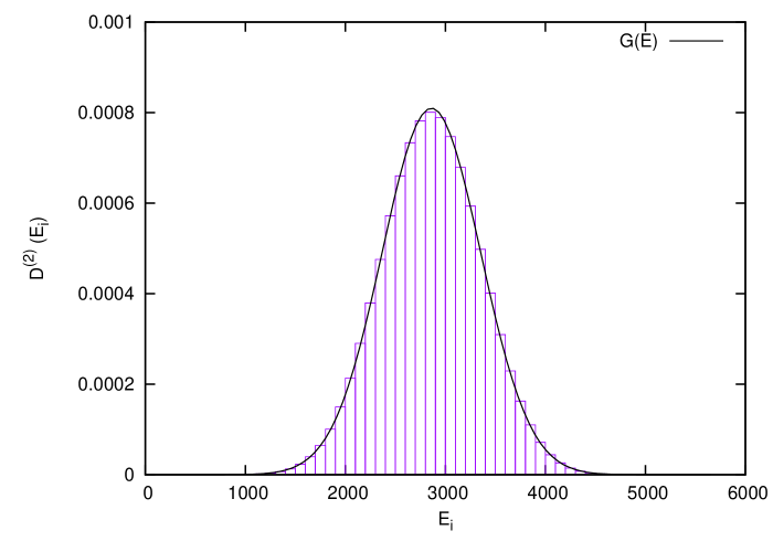
Figure 1: Continuous curve represents the Gaussian distribution $G(E)$ and the histogram represents the normalized level density distribution for the dispersion relation (4.3) with coefficients $f_{0,1}=1$, $f_{0,2}=-1$, $f_{1,1}=1$, drawn for the case $N=40$ and $m=2$.

From this figure it is evident that the histogram matches very well with the Gaussian distribution $G(E)$ in Eq. (2.3), where the values of $\mu$ and $\sigma^{2}$ are obtained by using Eqs. (4.4a) and (4.4b) respectively. Inserting the numerical values of $D^{(m)}(E_{i})$ in Eq. (4.1), subsequently we calculate the cumulative level density distribution $F(E)$ for the above mentioned case. In Fig.$2$ we plot $F(E)$ at equidistant points and also the error function $C(E)$ given in Eq. (4.2).

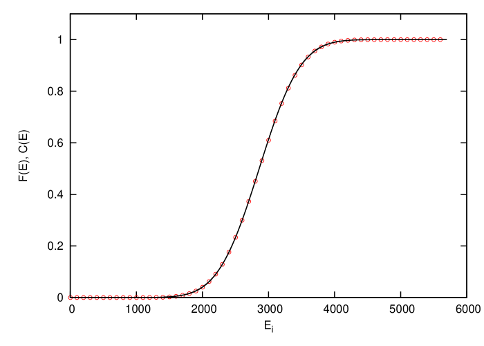
Figure 2: Continuous curve represents the error function $C(E)$, while the circles represent cumulative level density distribution $F(E)$ for the dispersion relation (4.3) with coefficients $f_{0,1}=1$, $f_{0,2}=-1$, $f_{1,1}=1$, drawn for the case $N=40$ and $m=2$.

Comparison from this figure shows that $F(E)$ and $C(E)$ are in excellent agreement with each other. We also calculate the mean square error (MSE) for this case and find it to be as low as $4.10\times 10^{-7}$. In Table 1 we present the values of such MSE, which are calculated by taking different sets of values of $f_{0,1},f_{0,2},f_{1,1}$ in the dispersion relation (4.3) for a wide range of $N$ (keeping the value of $m$ unchanged).

Sets of Parameters			$N=20$	$N=40$	$N=50$	$N=60$	$N=70$
$f_{0,1}$	$f_{0,2}$	$f_{1,1}$
$1$	$1$	$1$	$8.17\times 10^{-6}$	$1.18\times 10^{-6}$	$6.56\times 10^{-7}$	$4.08\times 10^{-7}$	$2.74\times 10^{-7}$
$1$	$-1$	$1$	$3.70\times 10^{-6}$	$4.10\times 10^{-7}$	$2.29\times 10^{-7}$	$1.44\times 10^{-7}$	$9.81\times 10^{-8}$
$1$	$2$	$1$	$1.01\times 10^{-5}$	$1.43\times 10^{-6}$	$7.95\times 10^{-7}$	$4.93\times 10^{-7}$	$4.93\times 10^{-7}$
$1$	$-1$	$2$	$2.46\times 10^{-6}$	$4.09\times 10^{-7}$	$2.33\times 10^{-7}$	$1.48\times 10^{-7}$	$1.00\times 10^{-7}$
$1$	$-1$	$3$	$3.07\times 10^{-6}$	$5.10\times 10^{-7}$	$2.90\times 10^{-7}$	$1.83\times 10^{-7}$	$1.24\times 10^{-7}$

Table 1: MSE for cumulative level density for the dispersion relation (4.3) with $m=2$

From this table we find that, for any particular choice of the three parameters, the MSE decreases steadily with the increase of $N$. This fact clearly indicates that for $m=2$ the level density for the dispersion relation (4.3) asymptotically follows the Gaussian distribution. By using the same numerical method and taking different values of $m$, we have also studied the level densities for the dispersion relation (4.3) as well as a few other polynomial type dispersion relations and found that such level densities tend to the Gaussian distribution in all cases.

5 Concluding remarks

By using the transfer matrix approach, we analytically show that the level density for a large class of 1D vertex models and $Y(sl_{m})$ Yangian invariant quantum spin chains, associated with polynomial type dispersion relations of the form (3.1), asymptotically follow the Gaussian distribution. The universal nature of the asymptotic forms given in Eqs. (3.29) and (3.31), which do not depend on the parameters or coefficients present in the dispersion relation, play a key role in our analysis. We also present some numerical evidence in support of our analytical result. This result clearly implies that the Gaussian character of the level density distributions for these type of models is very robust in nature and probably originates from the underlying Yangian quantum group symmetry, rather than any specific choice of the dispersion relation. As a by product of our study on the level density distribution, we derive Eqs. (3.26) and (3.32) which give general expressions for the order of variance and mean of the energy function respectively, for any polynomial type dispersion relation.

It is expected that the results obtained in this article would play an important role in investigating the density of spacings between consecutive energy levels of unfolded spectra for the class of Yangian invariant spin chains and 1D vertex models associated with polynomial type dispersion relations. It should be noted that, for calculating the density of spacings, the energy levels are usually taken from the unfolded spectrum which has an approximately uniform level density distribution [46]. Such unfolded spectrum can be generated from the raw spectrum through a transformation involving the level density of the raw spectrum. Since we have shown that level density of all Yangian invariant spin chains and 1D vertex models associated with polynomial type dispersion relations satisfy the Gaussian distribution, one can easily construct the corresponding unfolded spectra and analyze the density of level spacings for them [47]. It may also be interesting to study various thermodynamical properties and correlation functions for this type of Yangian invariant spin chains and vertex models through the transfer matrix approach.

References

- [1] B. Sutherland, Beautiful Models: 70 Years of Exactly Solved Quantum Many-Body Problems (World Scientific, Singapore, 2004).
- [2] V.E. Korepin, N.M. Bogoliubov, and A.G. Izergin, Quantum Inverse Scattering Method and Correlation Functions, Cambridge Monographs on Mathematical Physics, (Cambridge University Press, Cambridge, 1993).
- [3] F. H. L. Essler, H. Frahm, F. Göhmann, A. Klümper and V. E. Korepin, The One-Dimensional Hubbard Model (Cambridge University Press, Cambridge, 2005).
- [4] Z.N.C. Ha, Quantum Many-body Systems in one Dimension, volume 12 of Advances in Statistical Mechanics (World Scientific, Singapore, 1996).
- [5] F.D.M. Haldane, Phys. Rev. Lett. 60 (1988) 635.
- [6] B.S. Shastry, Phys. Rev. Lett. 60 (1988) 639.
- [7] A.P. Polychronakos, Phys. Rev. Lett. 70 (1993) 2329.
- [8] H. Frahm, J. Phys. A 26 (1993) L473.
- [9] A.P. Polychronakos, Nucl. Phys. B 419 (1994) 553.
- [10] H. Frahm and V.I. Inozemstsev, J. Phys. A.: Math. Gen. 27 (1994) L801.
- [11] J.C. Barba, F. Finkel, A. González-López and M.A. Rodríguez, Nucl. Phys. B 839 (2010) 499.
- [12] F.D.M. Haldane, Phys. Rev. Lett. 67 (1991) 937.
- [13] F. D. M Haldane, in Proc. 16th Taniguchi Symp., Kashikojima, Japan (1993), eds. A. Okiji and N. Kawakami (Springer, 1994).
- [14] B. A. Bernevig, V. Gurarie and S. H. Simon, J. Phys. A: Math. Theor. 42 (2009) 245206.
- [15] B. A. Bernevig and F.D.M. Haldane, Phys. Rev. Lett. 102 (2009) 066802.
- [16] N. Beisert, V. Dippel, M. Staudacher. JHEP 0407 (2004) 075.
- [17] D. Serban, M. Staudacher, JHEP 0406 (2004) 001.
- [18] N. Beisert, M. Staudacher, Nucl. Phys. B 727 (2005) 1.
- [19] T. Bargheer, N. Beisert, F. Loebbert, J. Phys. A 42 (2009) 285205.
- [20] D. Serban, J. Phys. A 44 (2011) 124001.
- [21] F. D. M. Haldane, Z.N.C. Ha, J.C. Talstra, D. Benard and V. Pasquier, Phys. Rev. Lett. 69 (1992) 2021.
- [22] D. Benard, M. Gaudin, F. D. M. Haldane, and V. Pasquier, J. Phys. A 26 (1993) 5219.
- [23] K.Hikami, Nucl. Phys. B 441 (1995) 530.
- [24] A. N. Kirilov, A. Kuniba, and T. Nakanishi, Commun. Math. Phys. 185 (1997) 441.
- [25] K. Hikami and B. Basu-Mallick, Nucl. Phys. B 566 (2000) 511.
- [26] K. Hikami, Exclusion Statistics and Chiral Partition Function, in “Physics and Combinatorics 2000”, eds. A. N. Kirilov and N. Liskova, pp 22-48.
- [27] B. Basu-Mallick, N. Bondyopadhaya, K. Hikami and D. Sen, Nucl. Phys. B 782 (2007) 276.
- [28] B. Basu-Mallick, N. Bondyopadhaya and D. Sen, Nucl. Phys. B 795 (2008) 596.
- [29] B. Basu-Mallick, Nucl. Phys. B 540 (1999) 679.
- [30] B. Basu-Mallick, H. Ujino and M. Wadati, Jour. Phys. Soc. Jpn. 68 (1999) 3219.
- [31] B. Basu-Mallick and N. Bondyopadhaya, Nucl. Phys. B 757 (2006) 280.
- [32] B. Sutherland, J. Math. Phys. 11 (1970) 3183.
- [33] R.J. Baxter, Phys. Rev. Lett. 26 (1971) 834.
- [34] A. Enciso, F. Finkel and A. González-López, Phys. Rev. E 82 (2010) 051117.
- [35] B. Basu-Mallick, N. Bondyopadhaya and K. Hikami, SIGMA 6 (2010) 091.
- [36] F. Finkel and A. González-López, Phys. Rev. B 72 (2005) 174411.
- [37] A. Enciso, F. Finkel, A. González-López, and M. A. Rodríguez, Nucl. Phys. B 707 (2005) 553.
- [38] B. Basu-Mallick, F. Finkel, and A. González-López, Nucl. Phys. B 812 (2009) 402.
- [39] J. C. Barba, F. Finkel, A. González-López, and M. A. Rodríguez, Phys. Rev. B 77 (2008) 214422.
- [40] J. C. Barba, F. Finkel, A. González-López, and M. A. Rodríguez, Europhys. Lett. 83 (2008) 27005.
- [41] J. C. Barba, F. Finkel, A. González-López, and M. A. Rodríguez, Nucl. Phys. B 806 (2009) 684.
- [42] W. Feller, An Introduction to Probability Theory and its Applications, 3rd ed., Vol.2 (John Wiley and Sons, New York, 1971).
- [43] N.G. de Bruijn, Asymptotic Methods in Analysis (North-Holland, Amsterdam, 1958).
- [44] H. Jeffreys and B. Jeffreys, Methods of Mathematical Physics, 3rd ed., (Cambridge University Press, England, 2000).
- [45] D. Knuth, ACM SIGACT News, Vol. 8, Issue 2 (1976) 18.
- [46] F. Haake, Quantum Signatures of Chaos, 2nd ed. (Springer-Verlag, Berlin, 2001).
- [47] B. Basu-Mallick, F. Finkel, and A. González-López, Under Preparation.