Variational calculation of ⁴He tetramer ground and excited states
using a realistic pair potential

Abstract

We calculated the ⁴He trimer and tetramer ground and excited states with the LM2M2 potential using our Gaussian expansion method (GEM) for ab initio variational calculations of few-body systems. The method has extensively been used for a variety of three-, four- and five-body systems in nuclear physics and exotic atomic/molecular physics. The trimer (tetramer) wave function is expanded in terms of symmetric three-(four-)body Gaussian basis functions, ranging from very compact to very diffuse, without assuming any pair correlation function. Calculated results of the trimer ground and excited states are in excellent agreement with the literature. Binding energies of the tetramer ground and excited states are obtained to be 558.98 mK and 127.33 mK (0.93 mK below the trimer ground state), respectively. We found that precisely the same shape of the short-range correlation ($r_{ij}\mathrel{\mathchoice{\lower 3.6pt\vbox{\halign{$\mathsurround=0pt\displaystyle\hfil#\hfil$\cr<\crcr\sim\crcr}}}{\lower 3.6pt\vbox{\halign{$\mathsurround=0pt\textstyle\hfil#\hfil$\cr<\crcr\sim\crcr}}}{\lower 3.6pt\vbox{\halign{$\mathsurround=0pt\scriptstyle\hfil#\hfil$\cr<\crcr\sim\crcr}}}{\lower 3.6pt\vbox{\halign{$\mathsurround=0pt\scriptscriptstyle\hfil#\hfil$\cr<\crcr\sim\crcr}}}}4$Å) in the dimer appear in the ground and excited states of trimer and tetramer. The overlap function between the trimer excited state and the dimer and that between the tetramer excited state and the trimer ground state are almost proportional to the dimer wave function in the asymptotic region (up to $\sim 1000$ Å). Also the pair correlation functions of trimer and tetramer excited states are almost proportional to the squared dimer wave function. We then come to propose a model which predicts the binding energy of the first excited state of ⁴He_N ($N\geq 3$) measured from the ⁴He_N-1 ground state to be nearly $\frac{N}{2(N-1)}B_{2}$ using the dimer binding energy $B_{2}$.

I INTRODUCTION

In early 1970’s, Efimov pointed out a possibility of having an infinite number of three-body bound states even when none exists in the separate two-body subsystems Efimov70 ; Efimov73 ; Efimov11 . This occurs when the two-body scattering length is much larger than the range of the two-body interaction. As a candidate of such three-body states, Efimov discussed about the famous Hoyle state Hoyle (the second $0^{+}$ state at 7.65MeV in the ¹²C nucleus) taking a model of three $\alpha$ particles (clusters of three ⁴He nuclei) as well as about the three-nucleon bound state (³H nuclei). In nuclear systems, the Borromean states, weakly bound three-body states though having no bound two-body subsystems, are familiar but not classified as Efimov states.

In atomic systems, triatomic ⁴He (trimer) have been expected to have bound states of Efimov type since the realistic ⁴He-⁴He interactions HFDHE2 ; LM2M2 ; TTY ; SAPT2 ; HFDB3FCI1 give a large ⁴He-⁴He scattering length ($\simeq 115$Å), much greater than the potential range ($\sim 10$Å), and a very small ⁴He dimer binding energy ($\simeq 1.3$ mK). (Experimentally, Ref. Grisenti2000 evaluated a scattering length of $104^{+8}_{-18}$ Å  and a binding energy of $1.1^{+0.3}_{-0.2}$ mK).

As is mentioned in recent reviews about the ⁴He trimer review-2009 ; review-Efimov (further references therein), i) a lot of three-body calculations using the realistic pair potentials have shown that the ⁴He trimer possesses two bound states with binding energies of nearly $126.4$ mK and $2.3$ mK, ii) it is already rather well established that, if the ⁴He trimer excited state exist, it should be Efimov nature, and iii) it is suggested that the ⁴He trimer ground state may be considered as an Efimov state since the ground- and excited-state binding energies move along the same universal scaling curve under any small deformation of the two-body potential (for details, see, e.g., Sec.III of Ref. Braaten03 ). Experimentally, the ⁴He trimer ground state has been observed in Ref. dimer-exp2005 to have the ⁴He-⁴He bond length of $11^{+4}_{-5}$ Å  in agreement with theoretical predictions, whereas a reliable experimental evidence for the ⁴He trimer excited state is still missing.

Only very recently, experimental evidences of Efimov trimer states have been reported in the work using the ultracold gases of cesium atoms cesium-Kramer ; cesium-Knoop , potasium atoms Potasium-Zaccanti , lithium-7 atoms Lithium-Gross ; Lithium-Pollack , and lithium-6 atoms Li6-Lompe ; Li6-Nakajima1 ; Li6-Nakajima2 ; Li6-Ottensen ; Li6-Williams , in which the two-body interaction between those alkali atoms was manipulated so as to tune the scattering length to values significantly greater than the potential range. These experiments have been accessing the study of a wide variety of interesting physical systems in the atomic and nuclear fields. Recently, the study extends to the Efimov physics and universality of four-atomic systems (tetramers).

Though the interactions between ⁴He atoms can not be manipulated, the study of ⁴He trimer using the realistic pair potentials has been providing fundamental information to the Efimov physics. Now it is one of the challenging subjects to precisely investigate the structure of ⁴He tetramer using the realistic ⁴He-⁴He potential.

So far there exist in the literature a large number of ⁴He trimer calculations Carbonell ; Kievsky01 ; Roudnev ; Lewerenz ; Bressanini ; Blume ; Das ; Pandha83 ; Gloeckle86 ; Carbonell93 ; Nielsen98 ; Roudnev00 ; Motovilov01 ; Kologanova04 ; Suno08 giving well converged results with the realistic ⁴He-⁴He interactions. However, calculations of the tetramer remain limited Carbonell ; Lewerenz ; Bressanini ; Blume ; Das ; in those papers, the binding energy of the tetramer ground state agrees well with each other, while that of the loosely bound excited state differs significantly from one another.

Thus the main purpose of the present paper is to perform accurate calculations of the ⁴He tetramer ground and excited states using a realistic ⁴He-⁴He interaction, the LM2M2 potential LM2M2 . We employ the Gaussian expansion method (GEM) for ab initio variational calculations of few-body systems Kamimura88 ; Kameyama89 ; Kamimura90 ; Hiyama03 . The method has been proposed and developed by the present authors and collaborators and applied to various types of three-, four- and five-body systems in nuclear physics and exotic atomic/molecular physics (cf. review papers Hiyama03 ; Hiyama09 ; Hiyama10 ).

Advantage of using the GEM for the ⁴He tetramer calculation in the presence of the strong short-range repulsive potential is as follows: Some 30000 symmetrized four-body Gaussian basis functions, ranging from very compact to very diffuse, are constructed on the full 18 sets of Jacobi coordinates without assuming any pair correlation function. They forms a nearly complete set in the finite coordinate space concerned, so that one can describe accurately both the short-range structure and the long-range asymptotic behavior (up to $\sim 1000$ Å) of the four-body wave function, which makes it possible to find new facets of ⁴He clusters.

We thus find that precisely the same shape of the short-range correlation ($r_{ij}\mathrel{\mathchoice{\lower 3.6pt\vbox{\halign{$\mathsurround=0pt\displaystyle\hfil#\hfil$\cr<\crcr\sim\crcr}}}{\lower 3.6pt\vbox{\halign{$\mathsurround=0pt\textstyle\hfil#\hfil$\cr<\crcr\sim\crcr}}}{\lower 3.6pt\vbox{\halign{$\mathsurround=0pt\scriptstyle\hfil#\hfil$\cr<\crcr\sim\crcr}}}{\lower 3.6pt\vbox{\halign{$\mathsurround=0pt\scriptscriptstyle\hfil#\hfil$\cr<\crcr\sim\crcr}}}}4$ Å) in dimer appears in the ground and excited states of trimer and tetramer. This gives a foundation to an a priori assumption that a two-particle correlation function (such as the Jastrow’s) so as to simulate the short-range part of the dimer wave function is incorporated in the trimer and tetramer wave functions from the beginning.

By illustrating the asymptotic behavior of the ⁴He trimer and tetramer, we discuss about an interesting relation between their excited-state wave functions and the dimer wave function. We then come to propose a ’dimerlike-pair’ model that predicts the binding energy of the first excited state of the $N$-cluster system, ⁴He_N, measured from the ground state of ⁴He_N-1 to be approximately $\frac{N}{2(N-1)}B_{2}$ using the dimer binding energy $B_{2}$.

We explicitly write the asymptotic form of the total wave function of ⁴He trimer (tetramer). The asymptotic normalization coefficient (ANC) Friar ; Kameyama89 ; Kievsky01 ; ANC1 ; ANC2 , namely the amplitude of tail function of the dimer-atom (trimer-atom) relative motion in the present case, is a quantity to reflect the internal structure of trimer (tetramer). Therefore, attention to the ANC might be useful when one intends to reproduce the non-universal variation of the ⁴He trimer (tetramer) states by means of parametrizing effective models beyond Efimov’s universal theory.

The paper is organized as follows: In Sec. II, we apply the GEM to the three-body calculation of the ⁴He trimer ground and excited states showing that the calculated results agree excellently with the literature. In Sec. III, the four-body calculation of the ⁴He tetramer ground and excited states is presented. Summary is given in Sec. IV.

II ⁴He trimer

The ⁴He trimer bound states have extensively been studied in many theoretical work using realistic potentials. Monte-Carlo, hyperspherical, variational and Faddeev techniques were used to calculate accurately the binding energies of the ground and excited states Carbonell ; Kievsky01 ; Roudnev ; Lewerenz ; Bressanini ; Blume ; Das ; Pandha83 ; Gloeckle86 ; Carbonell93 ; Nielsen98 ; Roudnev00 ; Suno08 ; Motovilov01 ; Kologanova04 (see also recent reviews review-2009 ; review-Efimov ). Nevertheless, in this section, we explain our Gaussian expansion method (GEM) and present the calculated result for the ⁴He trimer in order to demonstrate high accuracy of our calculation before we report our investigation of the ⁴He tetramer in the next section.

II.1 Three-body wave function

We take all the three sets of Jacobi coordinates (Fig. 1), ${\bf x}_{1}={\bf r}_{2}-{\bf r}_{3}$ and ${\bf y}_{1}={\bf r}_{1}-\frac{1}{2}({\bf r}_{2}+{\bf r}_{3})$ and cyclically for $({\bf x}_{2},{\bf y}_{2})$ and $({\bf x}_{3},{\bf y}_{3})$, ${\bf r}_{i}$ being the position vector of $i$th particle. Hamiltonian of the system is expressed as

$$H=-\frac{\hbar^{2}}{2\mu_{x}}\nabla^{2}_{x}-\frac{\hbar^{2}}{2\mu_{y}}\nabla^{2}_{y}+\sum_{1=i<j}^{3}V(r_{ij}),$$ (1)

where $\mu_{x}=\frac{1}{2}m$ and $\mu_{y}=\frac{2}{3}m$, $m$ being mass of a ⁴He atom. $V(r_{ij})$ is the two-body ⁴He-⁴He potential as a function of the pair distance ${\bf r}_{ij}={\bf r}_{j}-{\bf r}_{i}$.

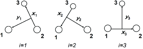
Figure 1: Three sets of the Jacobi coordinates for ⁴He trimer.

We calculate the three-body bound-state wave function, $\Psi_{3}$, which satisfies the Schrödinger equation

$$(H-E)\Psi_{3}=0.$$ (2)

Since we consider the ⁴He atom as a spinless boson, we expand the wave function of three identical spinless bosons in terms of $L^{2}$-integrable, fully symmetric three-body basis functions:

$$\quad\Psi_{3}=\sum_{\alpha=1}^{\alpha_{\rm max}}A_{\alpha}\Phi_{\alpha}^{\rm(sym)},$$ (3)

$$\Phi_{\alpha}^{\rm(sym)} = \Phi_{\alpha}({\bf x}_{1},{\bf y}_{1})+\Phi_{\alpha}({\bf x}_{2},{\bf y}_{2})+\Phi_{\alpha}({\bf x}_{3},{\bf y}_{3}).\qquad$$ (4)

It is of importance that those basis functions {$\Phi_{\alpha}^{\rm(sym)};\alpha=1,...,\alpha_{\rm max}$}, which are nonorthogonal to each other, are constructed on the full three sets of Jacobi coordinates; this makes the function space of $\{\Phi_{\alpha}^{\rm(sym)}$} quite wide.

The eigenenergies $E$ and amplitudes $A_{\alpha}$ of the ground and excited states are determined by the Rayleigh-Ritz variational principle:

$$\langle\>\Phi_{\alpha}^{\rm(sym)}\>|\>H-E\>|\>\Psi_{3}\>\rangle=0,$$ (5)

where $\alpha=1,...,\alpha_{\rm max}$. Eqs.(2.5) results in a generalized eigenvalue problem:

$$\sum_{\alpha^{\prime}=1}^{\alpha_{\rm max}}\big{[}{\cal H}_{\alpha,\alpha^{\prime}}-E\,{\cal N}_{\alpha,\alpha^{\prime}}\big{]}\,A_{\alpha^{\prime}}=0.\qquad$$ (6)

The matrix elements are written as

$${\cal H}_{\alpha,\alpha^{\prime}} = \langle\>\Phi_{\alpha}^{\rm(sym)}\>|\>H\>|\>\Phi_{\alpha^{\prime}}^{\rm(sym)}\>\rangle,$$ (7)

$${\cal N}_{\alpha,\alpha^{\prime}} = \langle\>\Phi_{\alpha}^{\rm(sym)}\>|\>\>1\>\>|\>\Phi_{\alpha^{\prime}}^{\rm(sym)}\>\rangle.$$ (8)

The lowest-lying two $S$-wave eigenstates, $\Psi_{3}^{(v)}(v=0,1)$, will be identified as the trimer ground $(v=0)$ and excited ($v=1$) states.

We express each basis function $\Phi_{\alpha}({\bf x}_{i},{\bf y}_{i})$ as a product of a function of ${\bf x}_{i}$ and that of ${\bf y}_{i}$:

$$\Phi_{\alpha}({\bf x}_{i},{\bf y}_{i})=\phi_{n_{x}l_{x}}(x_{i})\psi_{n_{y}l_{y}}(y_{i})\Big{[}Y_{l_{x}}({\widehat{\bf x}_{i}})Y_{l_{y}}({\widehat{\bf y}_{i}})\Big{]}_{JM},$$ (9)

where $\alpha$ specifies a set of quantum numbers

$$\alpha=\{n_{x}l_{x},n_{y}l_{y},JM\}$$

commonly for the components $i=1,2,3$. $J$ is the total angular momentum and $M$ is its $z$-component. In this paper, we consider the trimer bound states with $J=0$. Then, the totally symmetric three-body wave function requires $l_{x}=l_{y}={\rm even}$.

One of the most important issues of the present variational calculation is what type of radial shape we use for $\phi_{n_{x}l_{x}}(x_{i})$ and $\psi_{n_{y}l_{y}}(y_{i})$. The basis functions should be capable of precisely describing the strong short-range correlation (without assuming any correlation function a priori) and the long-range asymptotic behavior of very loosely bound states.

The GEM recommends two types of functions which are tractable in few-body calculations and work acculately. One is the Gaussian function and the other, more powerful one, is the complex-range Gaussian function Hiyama03 . In the next subsection, we introduce the former that was successfully used in our previous study (Sec. 3.1 of Ref. Hiyama03 ) of the ⁴He trimer ground and excited state with the use of the HFDHE2 potential HFDHE2 . The latter function is introduced in Sec.II.C.

II.2 Gaussian basis functions

The radial function $\phi_{n_{x}l_{x}}(x)$ in (2.9) is taken to be a Gaussian multiplied by $x^{l_{n_{x}}}$ (similarly for $\psi_{n_{y}l_{y}}(y)$ ):

$$\phi_{n_{x}l_{x}}(x)=x^{l_{x}}\>e^{-(x/x_{n_{x}})^{2}},\>\;$$ (10)

$$\psi_{n_{y}l_{y}}(y)=y^{l_{y}}\>e^{-(y/y_{n_{y}})^{2}},\>\;$$ (11)

where normalization constants are omitted for simplicity.

Setting of the ranges by stochastic or random choice does not seem suitable for describing the strong short-range correlation and the long-range asymptotic behavior of the wave function. Any intended choice of the ranges is necessary. The GEM recommends to set them in a geometric progression:

$$x_{n_{x}}=x_{1}\,a_{x}^{n_{x}-1}\quad\>(n_{x}=1,...,n_{x}^{\rm max})\;,$$ (12)

$$y_{n_{y}}=y_{1}\,a_{y}^{n_{y}-1}\quad\>(n_{y}=1,...,n_{y}^{\rm max}),\;$$ (13)

with common ratios $a_{x}>1$ and $a_{y}>1$. This greatly reduces the nonlinear parameters to be optimized. We designate a set of the geometric sequence by $\{n_{x}^{\rm max},\,x_{1},\,x_{n_{x}^{\rm max}}\}$ instead of $\{n_{x}^{\rm max},\,x_{1},\,a_{x}\}$ and similarly for $\{n_{y}^{\rm max},\,y_{1},\,y_{n_{y}^{\rm max}}\}$ , which is more convenient to consider the spatial distribution of the basis set. Optimization of the nonlinear range parameters is in principle by trial and error procedure but much of experiences and systematics have been accumulated in many studies using the GEM.

The basis functions {$\phi_{nl}$} have the following properties: i) They range from very compact to very diffuse, more densely in the inner region than in the outer one. While the basis functions with small ranges are responsible for describing the short-range structure of the system, the basis with longest-range parameters are for the asymptotic behavior. ii) They, being multiplied by normalization constants for $\langle\phi_{nl}\,|\,\phi_{nl}\rangle=1$, have a relation

$$\langle\phi_{n\,l}\,|\,\phi_{n+k\,l}\rangle=\left(\frac{2a^{k}}{1+a^{2k}}\right)^{l+3/2},$$ (14)

which tells that the overlap with the $k$-th neighbor is independent of $n$, decreasing gradually with increasing $k$.

We then expect that the coupling among the whole basis functions take place smoothly and coherently so as to describe properly both the short-range structure and long-range asymptotic behavior simultaneously. We note that a single Gaussian decays quickly as $x$ increases, but appropriate superposition of many Gaussians can decay even exponentially up to a sufficiently large distance. A good example is shown in Fig. 3 of Ref. Hiyama03 for the ⁴He dimer wave function (with the HFDHE2 potential) that is accurate up to $\sim\!1000$ Å  with the use of the nonlinear parameters {$n^{\rm max}=60$, $x_{1}=0.14$ Å and $x_{n^{\rm max}}=700$ Å } (the same-quality dimer wave function is seen in Fig. 2 below in Sec.II.D using the complex-range Gaussians with the LM2M2 potential).

A lot of successful examples of the three- and four-body GEM calculations are shown in review papers Hiyama03 ; Hiyama09 ; Hiyama10 and in papers of five-body calculations Pentaquark ; Hida . The examples includes our previous calculation of the ground and excited states of ⁴He trimer using the HFDHE2 potential; the binding energies were in good agreement with those given by a Feddeev-equation calculation Gloeckle86 . As for the trimer wave function, we showed, in Figs. 3, 13 and 14 in Ref.Hiyama03 , that the strong short-range correlation ($x\mathrel{\mathchoice{\lower 3.6pt\vbox{\halign{$\mathsurround=0pt\displaystyle\hfil#\hfil$\cr<\crcr\sim\crcr}}}{\lower 3.6pt\vbox{\halign{$\mathsurround=0pt\textstyle\hfil#\hfil$\cr<\crcr\sim\crcr}}}{\lower 3.6pt\vbox{\halign{$\mathsurround=0pt\scriptstyle\hfil#\hfil$\cr<\crcr\sim\crcr}}}{\lower 3.6pt\vbox{\halign{$\mathsurround=0pt\scriptscriptstyle\hfil#\hfil$\cr<\crcr\sim\crcr}}}}4$ Å) and asymptotic behavior (up to $x\sim 1000$ Å) of the trimer ground and excited states are simultaneously well described. Also, the three-body basis functions (2.9)–(2.13) together with the LM2M2 potential were used recently by Naidon, Ueda and one of the present authors (E. H.) Naidon2011 to study the universality and the three-body parameter of ⁴He trimers.

II.3 Complex-range Gaussian basis functions

Before we proceed to the calculation of the ⁴He tetramer ground and excited states, we improve the Gaussian shape of the basis functions so as to have more sophisticated (but still tractable) radial dependence. We then test the new basis in the calculation of the trimer states below.

In Ref. Hiyama03 , we proposed to improve the Gaussian shape by introducing complex range instead of the real one:

$$\phi_{nl}^{(\omega)}(x)=x^{l}\>e^{-(1+i\,\omega)(x/x_{n})^{2}},$$ (15)

where $n=1,...,n_{x}^{\rm max}$ and $x_{n}$ are given by (2.12). Using $\phi_{nl}^{(\pm\omega)}(x)$, we construct two kinds of real basis functions:

$$\phi_{nl}^{({\rm cos})}(x) = x^{l}\>e^{-(x/x_{n})^{2}}\,{\rm cos}\,\omega(x/x_{n})^{2}$$ (16)

$$= [\phi_{nl}^{(-\omega)}(x)+\phi_{nl}^{(\omega)}(x)]/2,$$

$$\phi_{nl}^{({\rm sin})}(x) = x^{l}\>e^{-(x/x_{n})^{2}}\,{\rm sin}\,\omega(x/x_{n})^{2}$$ (17)

$$= [\phi_{nl}^{(-\omega)}(x)-\phi_{nl}^{(\omega)}(x)]/2i,$$

where we usually take $\omega=1$. The three-body basis function $\Phi_{\alpha}({\bf x}_{i},{\bf y}_{i})$ in (2.9) is replaced by

$$\Phi_{\alpha}({\bf x}_{i},{\bf y}_{i})=\phi^{(^{\rm cos}_{\rm sin})}_{n_{x}l_{x}}(x)\,\psi_{n_{y}l_{y}}(y_{i})\Big{[}Y_{l_{x}}({\widehat{\bf x}_{i}})Y_{l_{y}}({\widehat{\bf y}_{i}})\Big{]}_{JM},$$ (18)

where $\alpha$ specifies a set

$$\alpha\equiv\mbox{ \{`cos' or `sin',}\,\omega,n_{x}l_{x},n_{y}l_{y},JM\}.$$ (19)

The new basis {$\phi^{(^{\rm cos}_{\rm sin})}_{n_{x}l_{x}}(x)$} apparently extend the function space from the old ones (2.10) since they have the oscillating components; see Sec.2.4 and Sec.2.5 of Ref. Hiyama03 for some examples taking this advantage in calculations of highly vibrational excited states (with $\sim$ 25 nodes) and scattering states. The sin-type basis (2.17) particularly work when the wave function is extremely suppressed at $x\sim 0$ due to the strongly repulsive short-range potential.

In the following calculations, we employ the new basis (2.16) and (2.17) for the $x$-space instead of (2.10), but keep (2.11) for the $y$-space.

Note that, when calculating the matrix elements (2.7) and (2.8) using $\phi_{nl}^{({\rm cos})}(x)$ and $\phi_{nl}^{({\rm sin})}(x)$, we explicitly take (2.15) and the right-most expression of (2.16) and (2.17) since the computation programming is almost the same as that for (2.10) though some of real variables are changed to complex ones.

A great advantage of the real- and complex-range Gaussian basis functions is that the calculation of matrix elements (2.7) and (2.8) is easily performed. As for the overlap and kinetic-energy matrix elements of the trimer (tetramer), all the six-(nine-)dimensional integrals give analytical expression. In the case of the potential matrix, we have analytical expression except for the one-dimensional numerical integral having the final form

$$\int_{0}^{\infty}x^{2m}\,e^{-\lambda x^{2}}\,V(x)\,x^{2}\,dx\,.$$ (20)

We explained, in Ref. Hiyama03 , various techniques to perform the three- and four-body matrix-element calculations as easily, accurately and rapidly as possible.

It is to be emphasized that the GEM few-body calculations need neither introduction of any a priori pair correlation function (such as the Jastrow function) nor separation of the coordinate space by $x<r_{c}$ and $x>r_{c}$, $r_{c}$ being the radius of a strongly repulsive core potential. Proper short-range correlation and asymptotic behavior of the total wave function are automatically obtained by solving the Schrödinger equation (2.2) using the above basis functions for ab initio calculations.

II.4 Pair interaction and ⁴He dimer

To describe the interaction between the ⁴He atoms, we employ one of the most widely used ⁴He-⁴He interactions, the LM2M2 potential by Aziz and Slaman LM2M2 . Use is made of $\frac{\hbar^{2}}{m}=12.12$ KÅ${}^{2}\,$ as the input mass of ⁴He atom. We can then precisely compare calculated results for the tetramer ground and excited states with those obtained by Lazauskas and Carbonell Carbonell who made a Faddeev-Yakubovsky (FY) equation calculation taking the same potential and ⁴He mass as above. Recently, the authors of Ref. newmass claim that a more precise value of $\frac{\hbar^{2}}{m}=12.11928$ KÅ${}^{2}\,$ should be employed. We shall additionally show the trimer and tetramer binding energies in the case of using this value.

Figure 2: Short-range structure (upper) and asymptotic behavior (lower) of the radial wave function $\Psi_{2}(x)$ of the ⁴He dimer obtained by using the complex-range Gaussian basis functions (2.21) and (2.22). The open circles stands for the exact asymptotic form. The dotted line (upper) illustrates the LM2M2 potential in arbitrary unit.

We calculated the ⁴He dimer binding energy, say $B_{2}$, and the wave function, $\Psi_{2}(\equiv\Psi_{2}(x)Y_{00}({\widehat{\bf x}}))$, using the same prescription as described above. We expanded $\Psi_{2}(x)$ with 100 basis functions of (2.16) and (2.17) as

$$\Psi_{2}(x)=\sum_{n=1}^{n_{x}^{\rm max}}\big{[}A_{n}^{\rm(cos)}\phi^{\rm(cos)}_{n0}(x)+A_{n}^{\rm(sin)}\phi^{\rm(sin)}_{n0}(x)\big{]}$$ (21)

with a parameter set

$$\{n_{x}^{\rm max}=50,\,x_{1}=0.5\,{\rm\AA},\,x_{n_{x}^{\rm max}}=600.0\,{\rm\AA},\,\omega=1.0\}.$$ (22)

We obtained $B_{2}=1.30348$ mK, $\sqrt{\langle x^{2}\rangle}=70.93$ Å, and $\langle x\rangle=52.00$ Å which are the same as those obtained in the literature. Experimentally, $\langle x\rangle=52\pm 4$ Å Grisenti2000 from which $B_{2}=1.1^{+0.3}_{-0.2}$ mK was estimated.

As shown in Fig. 2, both the strong short-range correlation ($x\mathrel{\mathchoice{\lower 3.6pt\vbox{\halign{$\mathsurround=0pt\displaystyle\hfil#\hfil$\cr<\crcr\sim\crcr}}}{\lower 3.6pt\vbox{\halign{$\mathsurround=0pt\textstyle\hfil#\hfil$\cr<\crcr\sim\crcr}}}{\lower 3.6pt\vbox{\halign{$\mathsurround=0pt\scriptstyle\hfil#\hfil$\cr<\crcr\sim\crcr}}}{\lower 3.6pt\vbox{\halign{$\mathsurround=0pt\scriptscriptstyle\hfil#\hfil$\cr<\crcr\sim\crcr}}}}4$ Å) and the asymptotic behavior of the dimer are well described. In the lower panel, $x\,\Psi_{2}(x)$ precisely reproduces the exact asymptotic shape $0.1498\,{\rm exp}(-\kappa_{2}x)$ (Å^-1/2) with $\kappa_{2}=\sqrt{mB_{2}}/\hbar=0.0104$ Å^-1 up to $x\!\sim\!\!1200$ Å  which is large enough for our discussions.

There are 30 basis functions whose Gaussian ranges $x_{n_{x}}<4$ Å, which is sufficiently dense to describe the short-range structure of the wave function precisely. An interesting issue is whether the same shape of the short-range correlation in Fig. 2 appear also in the trimer and tetramer ground and excited states without assuming any two-body correlation function.

II.5 Trimer bound states

We calculated the wave functions of the trimer ground state, $\Psi_{3}^{(0)}$, and the excited state, $\Psi_{3}^{(1)}$, and their binding energies, $B_{3}^{(0)}$ and $B_{3}^{(1)}$, respectively, as well as some mean values with the $\Psi_{3}^{(v)}$ $(v=0,1)$. Some of results are summarized in Table I together with those obtained in the literature. Our results excellently agree with those by Refs.Carbonell ; Kievsky01 ; Roudnev . The ⁴He-⁴He bond length in the trimer ground state was measured as $\langle r_{ij}\rangle=11^{+4}_{-5}$ Å Grisenti2000 , which is well explained by the calculations, $\langle r_{ij}\rangle=9.61$ Å.

Table 1: Mean values for ⁴He trimer ground and excited states with the use of the LM2M2 potential and $\frac{\hbar^{2}}{m}=12.12$ KÅ${}^{2}\,$. $B_{3}^{(v)}$ is the binding energy, $r_{ij}$ stands for interparticle distance and $r_{i{\rm G}}$ is the distance of a particle from the center-of-mass of the trimer. See text for the asymptotic normalization coefficient $C_{3}^{(v)}(v=0,1)$.

trimer	ground state
	present	Ref.Carbonell	Ref.Kievsky01	Ref.Roudnev
$B_{3}^{(0)}$ (mK)	126.40	126.39	126.4	126.40
$\langle T\rangle$ (mK)	1660.4	1658	1660
$\langle V\rangle$ (mK)	$-1786.8$	$-1785$	$-1787$
$\sqrt{\langle r^{2}_{ij}\rangle}$ (Å)	$10.96$	10.95	10.96
$\langle r_{ij}\rangle$ (Å)	$9.616$	9.612	9.610
$\langle r_{ij}^{-1}\rangle$ (Å${}^{-1})$	$0.134$	0.135
$\langle r_{ij}^{-2}\rangle$ (Å${}^{-2})$	$0.0228$	0.0230
$\sqrt{\langle r_{i{\rm G}}^{2}\rangle}$ (Å)	6.326		6.49	6.32
$C_{3}^{(0)}$(Å${}^{-\frac{1}{2}})$	0.562		0.567
trimer	excited state
	present	Ref.Carbonell	Ref.Kievsky01	Ref.Roudnev
$B_{3}^{(1)}$ (mK)	2.2706	2.268	2.265	2.2707
$\langle T\rangle$ (mK)	122.15	122.1	121.9
$\langle V\rangle$ (mK)	$-124.42$	$-124.5$	$-124.2$
$\sqrt{\langle r^{2}_{ij}\rangle}$ (Å)	$104.5$	104.3	101.9
$\langle r_{ij}\rangle$ (Å)	84.51	83.53	83.08
$\langle r_{ij}^{-1}\rangle$ (Å${}^{-1})$	0.0265	0.0267
$\langle r_{ij}^{-2}\rangle$ (Å${}^{-2})$	0.00216	0.00218
$\sqrt{\langle r_{i{\rm G}}^{2}\rangle}$ (Å)	60.33		58.8	59.3
$C_{3}^{(1)}$(Å${}^{-\frac{1}{2}})$	0.179		0.178

Those converged results were given by taking the symmetric three-body basis function {$\Phi_{\alpha}^{\rm(sym)};\alpha=1,...,\alpha_{\rm max}$} with $\alpha_{\rm max}=4400$, in which the shortest-range set is $(x_{1}\!=\!0.3\,$Å,$\,\,y_{1}\!=\!0.4\,$Å) and the longest-range one is $(x_{\rm max}\!=\!150\,$Å,$\,\,y_{\rm max}\!=\!600\,$Å). All the nonlinear parameters of the Gaussian basis set are listed in Table II.

Table 2: All the nonlinear parameters of the Gaussian basis functions used for the ⁴He-trimer states with $J=0\,(l_{x}=l_{y}$). Those in column a) are commonly for $\phi^{({\rm cos})}_{n_{x}l_{x}}(x)$ and $\phi^{({\rm sin})}_{n_{x}l_{x}}(x)$ and b) for $\psi_{n_{y}l_{y}}(y)$. Total number of the basis, $\alpha_{\rm max}$, is 4400.

a) $\phi^{({\rm cos})}_{n_{x}l_{x}}(x),\,\phi^{({\rm sin})}_{n_{x}l_{x}}(x)$						b) $\psi_{n_{y}l_{y}}(y)$
$l_{x}$	$n_{x}^{\rm max}$	$x_{1}$	$x_{n_{x}^{\rm max}}$	$\omega$		$l_{y}$	$n_{y}^{\rm max}$	$y_{1}$	$y_{n_{y}^{\rm max}}$	number
		[Å]	[Å]					[Å]	[Å]	of basis
0	22	0.3	150.0	1.0		0	50	0.4	600.0	2200
2	17	0.6	150.0	1.0		2	40	0.8	400.0	1360
4	14	0.8	130.0	1.0		4	30	1.0	200.0	840

There are neither additional parameter nor assumptions. The present calculation is so transparent that it is possible for the readers to repeat the calculation and check the results reported here. The parameters for the Gaussian ranges are in round numbers but further optimization of them do not improve the binding energies ($B_{3}^{(0)}=126.40$ mK and $B_{3}^{(1)}=2.2706$ mK) as long as we calculate them with five significant figures (cf. another check in Sec.II.H about the accuracy of the calculation).

Convergence of the binding energies $B_{3}^{(0)}$ and $B_{3}^{(1)}$ with respect to increasing partial waves $l_{x}(=l_{y})$ is shown in Table III in comparison with the Faddeev calculation by Lazauskas and Carbonell Carbonell . The case $l_{x_{\rm max}}=4$ is sufficient in the present work as long as the accuracy of five significant digits is required.

The convergence of the present result is more rapid than that of the Faddeev solution (the same will be seen in the tetramer calculation in Sec.III). The reason is that both the interaction and the wave function are truncated in the angular-momentum space $(l_{\rm max})$ in the Faddeev calculations, but the full interaction is included in the present calculation (with no partial-wave decomposition) though the wave function is truncated $(l_{\rm max})$. The difference of the convergence in the two calculation methods was precisely discussed in the case of the three nucleon bound states (³H and ³He nuclei) in our GEM calculation Kameyama89 ; Kamimura90 ; Hiyama03 and in a Faddeev calculation Payne93 ; for an illustration of the difference, see Fig. 15 in Ref. Hiyama03 . In this context, it is worth pointing out that, in Table 1, our result precisely agrees with another Faddeev calculation by Ref.Roudnev with no the partial wave decomposition.

Table 3: Convergence of the ⁴He trimer calculations with respect to the increasing maximum partial wave $(l_{\rm max})$. The four columns present trimer ground $(B_{3}^{(0)})$ and excited $(B_{3}^{(1)})$ state energies in comparison with those obtained by the Faddeev-equation calculation of Ref.Carbonell .

trimer	present			Ref.Carbonell
$l_{\rm max}$	$B_{3}^{(0)}$ (mK)	$B_{3}^{(1)}$ (mK)		$B_{3}^{(0)}$ (mK)	$B_{3}^{(1)}$ (mK)
0	121.00	2.2397		89.01	2.0093
2	126.39	2.2705		120.67	2.2298
4	126.40	2.2706		125.48	2.2622
8				126.34	2.2677
12				126.39	2.2680
14				126.39	2.2680

Use of the value $\frac{\hbar^{2}}{m}=12.11928$ KÅ${}^{2}\,$ newmass results in $B_{3}^{(0)}=126.499$ mK and $B_{3}^{(1)}=2.27787$ mK, while Ref. newmass gives $126.499$ mK and $2.27844$ mK, respectively. Calculation of the binding energy was also made perturbatively with $B_{3}=\frac{12.11928}{12.12}\langle\,T\,\rangle+\langle\,V\,\rangle$, where $\langle\,T\,\rangle$ and $\langle\,V\,\rangle$ are those obtained with $\frac{\hbar^{2}}{m}=12.12$ KŲ; this gives $B_{3}^{(0)}=126.498$ mK and $B_{3}^{(1)}=2.27787$ mK. The calculations below in Sec.II.F-H take $\frac{\hbar^{2}}{m}=12.12$ KŲ.

II.6 Short-range correlation and asymptotic behavior

In order to see how the present method describes the short-range structure of trimer, we calculated the pair correlation function (pair distribution function or two-body density) $P_{3}^{(v)}(x)$ defined by

$$P_{3}^{(v)}(x_{1})\,Y_{00}({\widehat{\bf x}}_{1})=\langle\,\Psi_{3}^{(v)}\,\!|\,\Psi_{3}^{(v)}\,\rangle_{{\bf y}_{1}},$$ (23)

where the symbol $\langle\quad\rangle_{{\bf y}_{1}}$ means the integration over ${\bf y}_{1}$ only. This integration gives an analytical expression owing to the use of the Gaussian basis functions; here, we explicitly rewrite $\Psi_{3}^{(v)}$ as a function of $({\bf x}_{1},{\bf y}_{1})$ by transforming the other coordinates $({\bf x}_{2},{\bf y}_{2})$ and $({\bf x}_{3},{\bf y}_{3})$ into $({\bf x}_{1},{\bf y}_{1})$. $P_{3}^{(v)}(x_{i})$ is independent of $i\,(=1,2,3)$ and is apparently normalized as $\int P_{3}^{(v)}(x)\,x^{2}{\rm d}x=1$. It presents the probability of finding two particles at an interparticle distance $x$.

In Fig. 3, short-range structure of $P_{3}^{(v)}(x)(v=0,1)$ is illustrated together with $P_{2}(x)(=|\Psi_{2}(x)|^{2})$ for the ⁴He dimer. The dashed line is for the trimer ground state $(v=0)$. The solid line for the excited state $(v=1)$ and the dotted line for the dimer have been multiplied by factors 14.5 and 6.0, respectively. It is of interest that precisely the same shape of the short-range correlation $(x\mathrel{\mathchoice{\lower 3.6pt\vbox{\halign{$\mathsurround=0pt\displaystyle\hfil#\hfil$\cr<\crcr\sim\crcr}}}{\lower 3.6pt\vbox{\halign{$\mathsurround=0pt\textstyle\hfil#\hfil$\cr<\crcr\sim\crcr}}}{\lower 3.6pt\vbox{\halign{$\mathsurround=0pt\scriptstyle\hfil#\hfil$\cr<\crcr\sim\crcr}}}{\lower 3.6pt\vbox{\halign{$\mathsurround=0pt\scriptscriptstyle\hfil#\hfil$\cr<\crcr\sim\crcr}}}}4$ Å) as seen in the dimer appears both in the trimer ground and excited states (the same will be seen in the tetramer ground and excited states in the next section). This gives a foundation to an a priori assumption that a two-particle correlation function (such as the Jastrow function) to simulate the short-range part of the dimer radial wave function $\Psi_{2}(x)$ is incorporated in the three-body wave function from the beginning.

Figure 3: Short-range structure of the pair correlation function $P_{3}^{(v)}(x)$ of the ⁴He trimer calculated by (2.23). The dashed line is for the trimer ground state $(v=0)$, the solid line for the excited state $(v=1)$ and the dotted line for the ⁴He dimer ($|\Psi_{2}(x)|^{2}$). The solid and dotted lines have been multiplied by factors 14.5 and 6.0, respectively, to be normalized at the peak. The same shape of the short-range correlation ($x\lesssim 4$ Å ) appears in the three states.

To investigate the trimer configuration in the asymptotic region where one atom is far from the other two, we calculate the overlap function ${\cal O}_{3}^{(v)}(y_{1})$ Friar ; Kameyama89 ; Kievsky01 ; ANC1 ; ANC2 to describe the overlap between the trimer wave function $\Psi_{3}^{(v)}(v=0,1)$ and the dimer one $\Psi_{2}({\bf x})$:

$${\cal O}_{3}^{(v)}(y_{1})\,Y_{00}({\widehat{\bf y}}_{1})=\langle\,\Psi_{2}({\bf x}_{1})\,|\,\Psi_{3}^{(v)}\,\rangle_{{\bf x}_{1}}.$$ (24)

In Fig. 4, we plot $y\,{\cal O}_{3}^{(v)}(y)$ for the ground and excited states. They should asymptotically satisfy

$$y\,{\cal O}_{3}^{(v)}(y)\stackrel{{\scriptstyle y\to\infty}}{{-\!\!\!\longrightarrow}}C_{3}^{(v)}{\rm exp}(-\kappa_{3}^{(v)}y),$$ (25)

where $\kappa_{3}^{(v)}$ is the binding wave number given by $\kappa_{3}^{(v)}\!=\!\sqrt{2\mu_{y}(B_{3}^{(v)}-B_{2})}/\hbar$ ($\kappa_{3}^{(0)}\!=\!0.117\!$ Å^-1, $\kappa_{3}^{(1)}\!=\!0.0103\!$ Å^-1). The amplitude $C_{3}^{(v)}$ is called the asymptotic normalzation coefficient (ANC) Friar ; Kameyama89 ; Kievsky01 ; ANC1 ; ANC2 defining the amplitude of the tail of the radial overlap function. The asymptotic functions (2.25) with $C_{3}^{(0)}\!=0.562$Å${}^{-\frac{1}{2}}$ and $C_{3}^{(1)}\!=0.179$Å${}^{-\frac{1}{2}}$ (see the open circles) are precisely reproduced by the dashed line ($v=0$) and the solid line ($v=1$), respectively, up to $y\!\sim\!1000$ Å , which demonstrates the accuracy of our wave functions in the asymptotic region. The values of $C_{3}^{(v)}$ agree with those given by Barletta and Kievsky Kievsky01 using a variational method with correlated hyperspherical harmonics functions (see Table I).

Figure 4: Overlap function ${\cal O}_{3}^{(v)}(y)$, multiplied by $y$, between the ⁴He trimer wave function $(v=0,1)$ and the dimer one, which is defined by (2.24). Open circles represent the fit of the asymptotic function (2.25) to ${\cal O}_{3}^{(v)}(y)$ using the asymptotic normalization coefficient $C_{3}^{(v)}$. The solid line $(v=1)$ is found to be parallel to the dotted line for the dimer wave function ($y\Psi_{2}(y)$).

The total three-body wave function $\Psi_{3}^{(v)}(v=0,1)$ is represented asymptotically as

$$\Psi_{3}^{(v)}\longrightarrow C_{3}^{(v)}\sum_{i=1}^{3}\Psi_{2}({\bf x}_{i})\frac{e^{-\kappa_{3}^{(v)}y_{i}}}{y_{i}}Y_{00}({\widehat{\bf y}_{i}}).\quad$$ (26)

The ANC, $C_{3}^{(v)}$, is a quantity to convey the interior structural information of the trimer to the asymptotic behavior. It is known, in the nuclear peripheral reactions where only the asymptotic tails of the wave functions of reacting particles contribute to the reaction process, the cross section is proportional to the squared ANC which can be measured in some specific systems ANC1 ; ANC2 ; Ogata-ANC-2006 . The idea of ANC might be available to the calculation of ⁴He atoms reactions such as ${\rm dimer}+{\rm dimer}\to{\rm trimer}+{\rm atom}$. Also, attention to the ANC might be useful when one intends to reproduce the non-universal variations of the trimer states by parametrizing effective models.

II.7 ’Dimerlike-pair’ model in asymptotic region

In Fig. 4, we find that the solid line ($v=1$) is parallel to the dotted line (dimer); namely, $\kappa_{3}^{(1)}(=0.0103$ Å^-1) is very close to $\kappa_{2}(=0.0104$ Å^-1). This agreement is not accidental, but is understandable from a model, which we refer to as a ’dimerlike-pair’ model, for the asymptotic behavior of the trimer excited state (Fig. 5a). The model tells that i) particle $a$, located far from $b$ and $c$ which are loosely bound (dimer), is little affected by the interaction between $b$ and $c$, ii) therefore, the pair $a$ and $b$ at a distance $x$ is asymptotically dimerlike, iii) since x $\simeq$ y asymptotically, the amplitude of particle $a$ along y is dimerlike, namely $\kappa_{3}^{(1)}\simeq\kappa_{2}$.

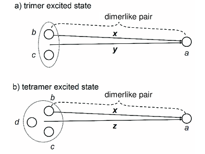
Figure 5: ’Dimerlike-pair’ model for the asymptotic behavior of the trimer and tetramer excited states (see text).

If this model is acceptable, we can predict that, in the asymptotic region, the pair correlation function of the trimer excited state, $x^{2}P_{3}^{(1)}(x)$, should decay exponentially with the same rate as that in the dimer ($x^{2}P_{2}(x)$). This is clearly seen in Fig. 6; the solid and dotted lines have almost the same exponentially-decaying rate of $2\kappa_{3}^{(1)}(\simeq 2\kappa_{2}$). The same evidence is seen in Figs. 3 and 14 of our previous calculation of the ⁴He trimer using the HFDHE2 potential reported in Ref. Hiyama03 .

Once we accept the dimerlike-pair model ($\kappa_{3}^{(1)}\simeq\kappa_{2}$), we can estimate $B_{3}^{(1)}$, the trimer excited-state binding energy, using $B_{2}$. With the use of the definitions of the binding wave numbers:

$$\kappa_{2} = \sqrt{2\mu_{x}B_{2}}/\hbar,$$ (27)

$$\kappa_{3}^{(1)} = \sqrt{2\mu_{y}(B_{3}^{(1)}-B_{2})}/\hbar,$$ (28)

where $\mu_{x}=\frac{1}{2}m$ and $\mu_{y}=\frac{2}{3}m$. Taking $\kappa_{3}^{(1)}\simeq\kappa_{2}$, we can then predict

$$B_{3}^{(1)}\simeq B_{2}+\frac{\mu_{x}}{\mu_{y}}B_{2}=\frac{7}{4}B_{2}=2.281\,{\rm mK},$$ (29)

which is close to 2.2706 mK by the present three-body calculation using the LM2M2 potential for which we have the ratio $B_{3}^{(1)}/B_{2}=1.74\,(\simeq 7/4)$.

In order to see a deviation of the ratio from 7/4 depending on the realistic potentials in the literature, we refer to $B_{3}^{(1)}/B_{2}=$ 1.59 Kievsky01 (SAPT2 SAPT2 ), 1.65 Suno08 ; newmass (SAPT2007 SAPT2007 ), 1.74 Kievsky01 ; Roudnev (TTY TTY ), 1.74 (LM2M2), 2.01 Motovilov01 (HFDHE2). The dimerlike-pair model provides a reason why the ratio $B_{3}^{(1)}/B_{2}$ is located around 7/4 in a narrow region of 1.6–2.0.

Figure 6: Asymptotic behavior of the pair correlation (distribution) function $P_{3}^{(v)}(x)$, multiplied by $x^{2}$, of the ⁴He trimer. The dashed line is for the trimer ground state $(v=0)$. The solid line for the excited state $(v=1)$ and the dotted line for the dimer are found to have almost the same exponentially-decaying rate, $2\kappa_{3}^{(1)}\simeq 2\kappa_{2}$.

We note that this model should be considered under the condition that the ⁴He atoms are interacting with a realistic pair potential and should not be discussed in any situation where a large deformation of the strength is posed to the potential (cf. a discussion in Sec.III of Ref. Braaten03 on the Efimov states in ⁴He trimer).

We try to apply the same model to the tetramer excited state (Fig. 5b) and predict its binding energy $B_{4}^{(1)}$. Asymptotically, particle $a$ decays from the trimer $(b+c+d$) as ${\rm exp}(-\kappa_{4}^{(1)}z)$ with

$$\kappa_{4}^{(1)}=\sqrt{2\mu_{z}(B_{4}^{(1)}-B_{3}^{(0)})}/\hbar,$$ (30)

where $\mu_{z}=\frac{3}{4}m$ is the reduce atom-trimer mass. Taking $\kappa_{4}^{(1)}\simeq\kappa_{2}$, we predict $B_{4}^{(1)}$ as

$$B_{4}^{(1)}\simeq B_{3}^{(0)}+\frac{\mu_{x}}{\mu_{z}}B_{2}=B_{3}^{(0)}+\frac{2}{3}B_{2}=127.27\,{\rm mK}$$ (31)

when employing the calculated values of $B_{3}^{(0)}$ and $B_{2}$ with LM2M2. In Sec.III, we make a four-body calculation of the tetramer with LM2M2 and check the above prediction of $B_{4}^{(1)}$.

II.8 Generalized eigenvalue problem

In this subsection, we discuss about a technical subject on a numerical trouble which arises when solving the generalized eigenvalue problem (2.6). This is due to the fact that the overlap matrix ${\cal N}$ becomes almost singular when a very large number of nonorthogonal basis functions $\{\Phi_{\alpha}^{\rm(sym)}$} employed. In this case, because of the non-negligible round-off error in double-precision computation ($\simeq$16 decimal digits), we may obtain no solution of (2.6) or a solution that includes some unphysically too deep erroneous bound state. In order to overcome this trouble, we took the following two steps:

Step i): we first diagonalize the overlap matrix ${\cal N}$:

$$\sum_{\alpha^{\prime}=1}^{\alpha_{\rm max}}{\cal N}_{\alpha,\alpha^{\prime}}C_{\alpha^{\prime}}^{(N)}=\nu_{N}C_{\alpha}^{(N)},$$ (32)

where $\alpha,N=1,...,\alpha_{{\rm max}}$. The eigenvalues $\nu_{N}$ are positive definite since ${\cal N}_{\alpha,\alpha^{\prime}}={\cal N}_{\alpha^{\prime},\alpha}$. We then define a new, symmetrized orthonormal basis set:

$${\widehat{\Phi}}_{N}^{\rm(sym)}=\frac{1}{\sqrt{\nu_{N}}}\sum_{\alpha=1}^{\alpha_{\rm max}}C_{\alpha}^{(N)}\Phi^{\rm(sym)}_{\alpha},$$ (33)

$$\langle{\widehat{\Phi}}_{N}^{\rm(sym)}\>|\>{\widehat{\Phi}}_{N^{\prime}}^{\rm(sym)}\rangle=\delta_{N,N^{\prime}},$$ (34)

where $N,N^{\prime}=1,...,\alpha_{\rm max}$. The generalized eigenvalue problem (2.6) are then equivalently converted into a standard eigenvalue problem:

$$\sum_{N^{\prime}=1}^{\alpha_{\rm max}}\big{[}{\widehat{\cal H}}_{N,N^{\prime}}-E\,{\delta}_{N,N^{\prime}}\big{]}\,{\widehat{A}}_{N^{\prime}}=0,$$ (35)

where $N=1,...,\alpha_{{\rm max}}$, and

$${\widehat{\cal H}}_{N,N^{\prime}}=\langle\>{\widehat{\Phi}}_{N}^{\rm(sym)}\>|\>H\>|\>{\widehat{\Phi}}_{N^{\prime}}^{\rm(sym)}\>\rangle.$$ (36)

Here, we arrange $\{{\widehat{\Phi}}_{N}^{\rm(sym)}\}$ in the decreasing order of $\nu_{N}$:

$$\nu_{1}>\nu_{2}>\cdot\cdot\cdot>\nu_{N}>\cdot\cdot\cdot>\nu_{\alpha_{\rm max}}.$$ (37)

When the nonorthogonality among the basis functions {$\Phi_{\alpha}^{\rm(sym)}$} is very large, some of $\nu_{N}$ become extremely small and therefore the large factor $1/\sqrt{\nu_{N}}$ may cause a serious cancellation in the summation in (2.33). Since the present calculation is performed by double-precision computation, such a large cancellation may generate a substantial round-off error in (2.33) and hence in the matrix elements (2.36). This may give rise to some erroneous eigenstates in (2.35) that have unphysically huge binding energies.

Table 4: Stability of the calculated trimer binding energies of the lowest-lying two states against decreasing number (${\widehat{N}}_{\rm max}$) of symmetrized orthonormal three-body basis functions {${\widehat{\Phi}}_{N}^{\rm(sym)}$} of Eq.(2.33). This assures accuracy of the conclusion $B_{3}^{(0)}\!=\!126.40$ mK and $B_{3}^{(1)}\!=\!2.2706$ mK in Table  I.

${\widehat{N}}_{\rm max}$	$(\Delta{\widehat{N}}_{\rm max})$	$B_{3}^{(0)}$ (mK)	$B_{3}^{(1)}$ (mK)
3250	$-$	$\quad 126.3999\quad$	$2.270606$
3240	$(-10)$	$126.3998$	$2.270605$
3200	$(-50)$	$126.3995$	$2.270602$
3150	$(-100)$	$126.3991$	$2.270594$
2950	$(-300)$	$126.3975$	$2.270533$
2750	$(-500)$	$126.3954$	$2.270484$
2250	$(-1000)$	$126.3657$	$2.270163$

Step ii): We therefore omit such members of {${\widehat{\Phi}}_{N}^{\rm(sym)}$} that have too small $\nu_{N}$. The binding energies of such unphysical states decreases quickly as the basis size is reduced. Finally, we reach an appropriate size, say ${\widehat{N}}_{\rm max}$, of the basis {${\widehat{\Phi}}_{N}^{\rm(sym)}$} for which those unphysical states have disappeared from the low-energy region, and energies of the lowest-lying (deepest) states take physically reasonable values. It is to be emphasized that the binding energies of so-obtained lowest-lying physical states are stable against further reduction of ${\widehat{N}}_{\rm max}$.

Table IV explicitly demonstrates Step ii). We start with $\alpha_{\rm max}=4400$ basis functions {$\Phi_{\alpha}^{\rm(sym)}$} whose parameters are given in Table II. When the size of the new basis {${\widehat{\Phi}}_{N}^{\rm(sym)}$} is reduced from $\alpha_{\rm max}$ to ${\widehat{N}}_{\rm max}=3250$ according to (2.37), the solution of (2.35) has come to include no unphysical state and give the binging energies $B_{3}^{(0)}=126.3999$ mK and $B_{3}^{(1)}=2.270606$ mK for the lowest two states. By checking the stability of the energy values against further decreasing ${\widehat{N}}_{\rm max}$, we verify the values of $B_{3}^{(0)}=126.40$ mK and $B_{3}^{(1)}=2.2706$ mK in Table I.

III ⁴He Tetramer

Calculation of the ⁴He tetramer using realistic potentials has been performed in Refs. Carbonell ; Lewerenz ; Bressanini ; Blume ; Das . Although binding energy of the ground state obtained in the papers agrees well with each other ($\sim\!558$ mK), that of the loosely bound excited state differs significantly from each other; namely, the binding energy with respect to the trimer ground state (126.4 mK) is given as 1.1 mK by the Faddeev-Yakubovski (FY) equations method Carbonell , 6.6 mK by Monte Carlo methods combined with the adiabatic hyperspherical approximation Blume and 52 mK recently by using a method of the correlated potential harmonic basis functions Das . Though the Faddeev result (1.1 mK) seems to the present authors the most accurate, the excited state was not solved as a bound-state problem in Ref. Carbonell but the result was extrapolated from the atom-trimer scattering phase shifts.

Thus the purpose of this section is to perform, using the same LM2M2 potential as in Ref. Carbonell , accurate bound-state calculation of the tetramer excited state, not only giving a precise binding energy but also describing the short-range correlation and the asymptotic behavior of the wave function properly.

The GEM has extensively been employed in bound-state calculations of various four-body systems in nuclear and hypernuclear physics (cf. review papers Hiyama03 ; Hiyama09 ; Hiyama10 ). Extension from three-body GEM calculations to four-body ones in the presence of strong short-range repulsion is a familiar subject in nuclear physics. For example, the study of three-nucleon bound states (³H and ³He nuclei) in Ref. Kameyama89 was extended to that of four-nucleon ground state (⁴He nucleus, $J^{\pi}=0^{+}$) Kamada01 and the first excited, very diffuse state ($J^{\pi}=0^{+}$) Hiyama03second . The study of the three-$\alpha$-particle system (¹²C nucleus) Hiyama03 ; Funaki ; Kurokawa was extended to that of the four-$\alpha$-particle system (¹⁶O nucleus) Funaki with the strongly repulsive Pauli-blocking projection operator on the $\alpha$-$\alpha$ motion. Therefore, extension of the ⁴He trimer calculation to the tetramer one is straightforward on account of those experiences.

III.1 Method

We take two types of Jacobi coordinate sets, K-type and H-type (Fig. 7). Namely, for K-type, ${\bf x}_{1}={\bf r}_{2}-{\bf r}_{1}$, ${\bf y}_{1}={\bf r}_{3}-\frac{1}{2}({\bf r}_{1}+{\bf r}_{2})$ and ${\bf z}_{1}={\bf r}_{4}-\frac{1}{3}({\bf r}_{1}+{\bf r}_{2}+{\bf r}_{3})$ and cyclically for $\{{\bf x}_{i},{\bf y}_{i},{\bf z}_{i};\,i=2,...,12\}$ by the symmetrization between the four particles. For H-type, ${\bf x}_{13}={\bf r}_{2}-{\bf r}_{1}$, ${\bf y}_{13}={\bf r}_{4}-{\bf r}_{3}$, ${\bf z}_{13}=\frac{1}{2}({\bf r}_{3}+{\bf r}_{4})-\frac{1}{2}({\bf r}_{1}+{\bf r}_{2})$ and cyclically for $\{{\bf x}_{i},{\bf y}_{i},{\bf z}_{i};\,i=14,...,18\}$. An explicit illustration of the totally 18 sets of the rearrangement Jacobi coordinates of four-body systems is seen in Fig. 18 of Ref. Hiyama03 .

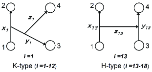
Figure 7: Jacobi coordinates, K-type and H-type, for the ⁴He tetramer. Symmetrization of the four particles generates the sets $i=1,...,12$ (K-type) and $i=13,...,18$ (H-type).

The total four-body wave function $\Psi_{4}$ is to be obtained by solving the Schödinger equation

$$(H-E)\Psi_{4}=0$$ (38)

with the Hamiltonian

$$H=-\frac{\hbar^{2}}{2\mu_{x}}\nabla^{2}_{x}-\frac{\hbar^{2}}{2\mu_{y}}\nabla^{2}_{y}-\frac{\hbar^{2}}{2\mu_{z}}\nabla^{2}_{z}+\sum_{1=i<j}^{4}V(r_{ij}),$$ (39)

where $\mu_{x}=\frac{1}{2}m$, $\mu_{y}=\frac{2}{3}m$ and $\mu_{z}=\frac{3}{4}m$ on the K-type coordinates, and $\mu_{x}=\mu_{y}=\frac{1}{2}m$ and $\mu_{z}=m$ on the H-type ones.

$\Psi_{4}$ is expanded in terms of the symmetrized $L^{2}$-integrable K-type and H-type four-body basis functions:

$$\Psi_{4}=\sum_{{\alpha_{\rm K}}=1}^{\alpha_{\rm K}^{\rm max}}A^{({\rm K})}_{\alpha_{\rm K}}\Phi^{({\rm sym;K})}_{\alpha_{\rm K}}+\sum_{{\alpha_{\rm H}}=1}^{\alpha_{\rm H}^{\rm max}}A^{({\rm H})}_{\alpha_{\rm H}}\Phi^{({\rm sym;H})}_{\alpha_{\rm H}},$$ (40)

with

$$\Phi_{\alpha_{\rm K}}^{({\rm sym;K})} = \sum_{i=1}^{12}\Phi^{({\rm K})}_{\alpha_{\rm K}}({\bf x}_{i},{\bf y}_{i},{\bf z}_{i}),$$ (41)

$$\Phi_{\alpha_{\rm H}}^{({\rm sym;H})} = \sum_{i=13}^{18}\Phi^{({\rm H})}_{\alpha_{\rm H}}({\bf x}_{i},{\bf y}_{i},{\bf z}_{i}),$$ (42)

in which $\Phi({\bf x}_{i},{\bf y}_{i},{\bf z}_{i})$ is a function of $i$-th set of Jacobi coordinates. It is of importance that $\Phi_{\alpha_{\rm K}}^{({\rm sym;K})}$ and $\Phi_{\alpha_{\rm H}}^{({\rm sym;H})}$ are constructed on the full 18 sets of Jacobi coordinates; this makes the function space of the basis quite wide.

The eigenenergies $E$ and amplitudes $A_{\alpha_{\rm K}}^{\rm(K)}(A_{\alpha_{\rm H}}^{\rm(H)})$ are determined by the Rayleigh-Ritz variational principle:

$$\langle\>\Phi_{\alpha_{\rm K}}^{({\rm sym;K})}\>|\>H-E\>|\>\Psi_{4}\>\rangle=0,$$ (43)

$$\langle\>\Phi_{\alpha_{\rm H}}^{({\rm sym;H})}\>|\>H-E\>|\>\Psi_{4}\>\rangle=0,$$ (44)

where $\alpha_{\rm K}=1,...,\alpha_{\rm K}^{\rm max}$ and $\alpha_{\rm H}=1,...,\alpha_{\rm H}^{\rm max}$. This set of equations results in a generalized eigenvalue problem:

$$\sum_{c^{\prime}={\rm K,H}}\;\;\sum_{\alpha_{\rm c^{\prime}}=1}^{\alpha_{\rm c^{\prime}}^{\rm max}}\Big{[}{\cal H}_{{\alpha_{\rm c}},{\alpha_{\rm c^{\prime}}}}^{\rm(c,c^{\prime})}-E\,{\cal N}_{{\alpha_{\rm c}},{\alpha_{\rm c^{\prime}}}}^{\rm(c,c^{\prime})}\Big{]}\>A_{\alpha_{\rm c^{\prime}}}^{\rm(c^{\prime})}=0,$$ (45)

where ${\rm c}={\rm K,H}$ and $\alpha_{\rm c}=1,...,\alpha_{\rm c}^{\rm max}$. The matrix elements are given by

$${\cal H}_{{\alpha_{\rm c}},{\alpha_{\rm c^{\prime}}}}^{\rm(c,c^{\prime})} = \langle\>\Phi_{\alpha_{\rm c}}^{\rm(c)}\>|\>H\>|\>\Phi_{\alpha_{\rm c^{\prime}}}^{\rm(c^{\prime})}\>\rangle,$$ (46)

$${\cal N}_{{\alpha_{\rm c}},{\alpha_{\rm c^{\prime}}}}^{\rm(c,c^{\prime})} = \langle\>\Phi_{\alpha_{\rm c}}^{\rm(c)}\>|\>\;1\>\;|\>\Phi_{\alpha_{\rm c^{\prime}}}^{\rm(c^{\prime})}\>\rangle.$$ (47)

Up to here is the most general way of variational calculations for bound states of identical spinless four particles.

We describe the basis function $\Phi^{({\rm K})}_{\alpha_{\rm K}}(\Phi^{({\rm H})}_{\alpha_{\rm H}})$ in the form

$$\Phi^{({\rm K})}_{\alpha_{\rm K}}({\bf x}_{i},{\bf y}_{i},{\bf z}_{i})=\phi^{(^{\rm cos}_{\rm sin})}_{n_{x}l_{x}}(x_{i})\,\phi_{n_{y}l_{y}}(y_{i})\,\varphi_{n_{z}l_{z}}(z_{i})$$

$$\times\Big{[}\big{[}Y_{l_{x}}({\widehat{\bf x}_{i}})Y_{l_{y}}({\widehat{\bf y}_{i}})\big{]}_{\Lambda}Y_{l_{z}}({\widehat{\bf z}_{i}})\Big{]}_{JM},$$

$$(i=1,...,12)$$ (48)

$$\Phi^{({\rm H})}_{\alpha_{\rm H}}({\bf x}_{i},{\bf y}_{i},{\bf z}_{i})=\phi^{(^{\rm cos}_{\rm sin})}_{n_{x}l_{x}}(x_{i})\,\psi_{n_{y}l_{y}}(y_{i})\,\varphi_{n_{z}l_{z}}(z_{i})$$

$$\times\Big{[}\big{[}Y_{l_{x}}({\widehat{\bf x}_{i}})Y_{l_{y}}({\widehat{\bf y}_{i}})\big{]}_{\Lambda}Y_{l_{z}}({\widehat{\bf z}_{i}})\Big{]}_{JM},$$

$$(i=13,...,18)$$ (49)

where $\alpha_{\rm K}$ specifies a set

$$\!\!\!\alpha_{\rm K}\equiv\mbox{ \{`cos' or `sin',}\,\omega,n_{x}l_{x},n_{y}l_{y},n_{z}l_{z},\Lambda,JM\},$$ (50)

which is commonly for the components $i=1,...,12$; and similarly for $\alpha_{\rm H}$ commonly for $i=13,...,18$.

Since we consider the case of $J=0$ in this paper, the totally symmetric four-body wave function requires i) $l_{x}={\rm even}$, $l_{y}+l_{z}={\rm even}$ and $\Lambda=l_{z}$ for the K-type basis and ii) $l_{x}={\rm even}$, $l_{y}={\rm even}$ and $\Lambda=l_{z}={\rm even}$ for the H-type basis.

In (3.11) and (3.12), the radial functions are assumed, as in Sec.II, to be

$$\phi^{(^{\rm cos}_{\rm sin})}_{n_{x}l_{x}}(x)=x^{l_{x}}\>e^{-(x/x_{n_{x}})^{2}}\times\big{\{}\,^{{\rm cos}\,\omega(x/x_{n_{x}})^{2}}_{{\rm sin}\,\omega(x/x_{n_{x}})^{2}}\;,\quad$$ (51)

$$\psi_{n_{y}l_{y}}(y)=y^{l_{y}}\>e^{-(y/y_{n_{y}})^{2}},\>\;$$ (52)

$$\varphi_{n_{z}l_{z}}(z)=z^{l_{z}}\>e^{-(z/z_{n_{z}})^{2}}\>\;$$ (53)

with geometric sequences of the Gaussian ranges:

$$x_{n_{x}}=x_{1}\,a_{x}^{n_{x}-1}\quad\>(n_{x}=1,...,n_{x}^{\rm max})\;,$$ (54)

$$y_{n_{y}}=y_{1}\,a_{y}^{n_{y}-1}\quad\>(n_{y}=1,...,n_{y}^{\rm max}),\;$$ (55)

$$z_{n_{z}}=z_{1}\,a_{z}^{n_{z}-1}\quad\>(n_{z}=1,...,n_{z}^{\rm max}).\;$$ (56)

In (3.15), the ’cos(sin)’-type function is not adopted for $\psi_{n_{y}l_{y}}(y)$ of the H-type basis though $y$ is the distance between two particles. This is because the ’cos(sin)’-type basis for the $x$-coordinate are applied to all the pairs of H-type by the symmetrization of the four particles.

In the tetramer calculation, the total number, $\alpha_{\rm max}=\alpha_{\rm K}^{\rm max}+\alpha_{\rm H}^{\rm max}$, of the symmetrized four-body basis functions (3.4) and (3.5) amounts to $\alpha_{\rm max}\sim$ 30000, ranging from very compact to very diffuse, to obtain a well converged solution. Since the nonorthogonality among those basis functions is too large to solve directly the generalized eigenvalue problem (3.8), we take the same two-step method as described in Sec.II.H in the trimer calculation. We finally solve the same type of standard eigenvalue problem as (2.35) using the symmetric orthonormal four-body basis functions, $\{{\widehat{\Phi}}^{({\rm sym})}_{N};N=1,...,{\widehat{N}}_{\rm max}\}$, in which the basis with too small $\nu_{N}$ have been omitted.

III.2 Binding energy

In the calculation of the ⁴He-tetramer ground state $\Psi_{4}^{(0)}$ and the excited state $\Psi_{4}^{(1)}$, the converged result was obtained by employing the symmetric four-body basis functions of $\alpha_{\rm max}=29056$ with $l_{\rm max}=4$. Table V shows the convergence of the binding energies of the tetramer ground $(B_{4}^{(0)})$ and excited $(B_{4}^{(1)})$ states with respect to increasing $l_{\rm max}$. Column ’K+H’ is the result with both the K-type and H-type basis functions in (3.3), and column ’(K)’ is that with the K-type basis only.

Contribution from the K-type basis is dominant, but that from the H-type is sizable. Without the latter the excited state does not become bound ($B_{4}^{(1)}<B_{3}^{(0)}=126.40$ mK) even for $l_{\rm max}=4$. Since both type bases are not orthogonal to each other, the role of H-type one can be substituted in principle by the K-type one if a very large $l_{\rm max}$ is employed. But, this is not practical; use of both types of bases is essentially important.

As seen in Table V, convegence of the binding energies with increasing $l_{\rm max}$ is more rapid in our calculation than that in the FY-equations calculation Carbonell . The reason of this difference in the conversion is the same as that mentioned in the trimer calculation (Sec.II.E).

Table 5: Convergence of ⁴He tetramer calculations with respect to the increasing maximum partial wave $(l_{\rm max})$. $B_{4}^{(0)}$ and $B_{4}^{(1)}$ are the binding energies of the ground and excited states, respectively. Column ’K+H’ is the results with both the K-type and H-type basis functions in (3.3) and column ’(K)’ is that with the K-type basis only. The excited state is unbound ($B_{4}^{(1)}<B_{3}^{(0)}=126.40$ mK) in the cases denoted by the symbol ’ $-$ ’. For comparison, $B_{4}^{(0)}$ obtained by the FY-equations calculation Carbonell is listed in the last column. The LM2M2 potential is employed.

tetramer	present						Ref.Carbonell
	$B_{4}^{(0)}$ (mK)			$B_{4}^{(1)}$ (mK)			$B_{4}^{(0)}$ (mK)
$l_{\rm max}$	K+H	( K )		K+H	( K )
0	500.71	(185.96)		$-$	( $-$ )		348.8
2	558.29	(508.62)		127.24	( $-$ )		505.9
4	558.98	(532.56)		127.33	( $-$ )		548.6
6							556.0
8							557.7

Table 6: Nonlinear parameters of the four-body Gaussian basis functions, (3.11)–(3.19), used for the ⁴He tetramer ground and excited states with $J=0\,(\Lambda=l_{z})$ in the case of $l_{\rm max}=2$ with 23504 basis functions (cf. Table V). In the leftmost column, K(H) stands for the K-type (H-type) basis. We take $\omega=1.0$ in (3.14).

	$\phi^{({\rm cos})}_{n_{x}l_{x}},\phi^{({\rm sin})}_{n_{x}l_{x}}$					$\psi_{n_{y}l_{y}}$					$\varphi_{n_{z}l_{z}}$
	$l_{x}$	$n_{x}^{\mbox{\tiny{\rm max}}}$	$x_{1}$	$x_{n_{x}^{\rm max}}$		$l_{y}$	$n_{y}^{\mbox{\tiny{\rm max}}}$	$y_{1}$	$y_{n_{y}^{\rm max}}$		$l_{z}$	$n_{z}^{\mbox{\tiny{\rm max}}}$	$z_{1}$	$z_{n_{z}^{\rm max}}$
			[Å]	[Å]				[Å]	[Å]				[Å]	[Å]
K	0	14	0.2	20.0		0	15	0.8	50.0		0	20	0.8	400.0
K	2	12	0.4	20.0		2	14	0.8	40.0		0	16	0.8	300.0
K	0	8	0.3	6.0		2	8	0.8	6.0		2	8	1.0	6.0
K	2	6	0.3	6.0		0	8	0.8	6.0		2	8	1.0	6.0
K	0	8	0.3	6.0		1	8	0.8	6.0		1	8	1.0	6.0
K	2	6	0.4	6.0		1	6	0.8	6.0		1	8	1.0	6.0
K	2	6	0.5	6.0		2	8	0.8	6.0		2	8	1.0	6.0
H	0	12	0.3	20.0		0	12	0.4	16.0		0	14	0.8	25.0
H	2	6	0.6	6.0		2	6	0.8	6.0		0	8	1.0	6.0
H	0	6	0.3	6.0		2	6	0.8	6.0		2	8	1.0	6.0
H	2	6	0.6	6.0		0	6	0.8	6.0		2	8	1.0	6.0
H	2	6	0.6	6.0		2	6	0.8	6.0		2	8	1.0	6.0

Table 7: Stability of the calculated binding energies of the ⁴He tetramer ground and excited states with respect to the number (${\widehat{N}}_{\rm max}$) of the symmetrized orthonormal four-body basis functions corresponding to {${\widehat{\Phi}}_{N}^{\rm(sym)}$} in Eq.(2.33) in the case of $l_{\rm max}=4$ with the LM2M2 potential. This concludes $B_{4}^{(0)}=558.98$ mK and $B_{4}^{(1)}=127.33$ K.

${\widehat{N}}_{\rm max}$	$(\Delta{\widehat{N}}_{\rm max})$	$B_{4}^{(0)}$ (mK)	$B_{4}^{(1)}$ (mK)
24800	$-$	$\quad 558.983\quad$	$127.326$
24790	$(-10)$	$558.981$	$127.326$
24780	$(-20)$	$558.980$	$127.326$
24750	$(-50)$	$558.977$	$127.326$
24700	$(-100)$	$558.975$	$127.325$
24300	$(-500)$	$558.954$	$127.323$
23800	$(-1000)$	$558.924$	$127.320$

In Table VI we list the nonlinear parameters of the four-body Gaussian basis functions, (3.11)–(3.19), in the case of $l_{\rm max}=2$ with 23504 basis functions (cf. Table V) to avoid too long listing for $l_{\rm max}=4$. The range parameters are given in round numbers but further optimization of them do not improve the binding energies as long as we calculate them with five significant figures.

When solving the generalized eigenvalue problem (3.8), we take the same two-step method as mentioned in Sec.II.H. Table VII shows stability of the binding energes of the ground and excited states $(B_{4}^{(v)},v=0,1)$ against the decreasing number ${\widehat{N}}_{\rm max}$ of the symmetrized orthonormal four-body basis functions corresponding to {${\widehat{\Phi}}_{N}^{\rm(sym)}$} in Eq.(2.33).

Calculated binding energies and some of mean values of the tetramer ground and excited states are summerized in Table VIII(a) in comparison with those obtained by Lazauskas and Carbonell Carbonell with the FY-equations method in which the excited state was not obtained by a direct bound-state calculation but the binding energy (127.5 mK) was extrapolated from the atom-trimer scattering calculations. Our result of $B_{4}^{(1)}=127.33$ mK, which is very closed to $B_{4}^{(1)}$ in Ref.Carbonell , confirms the existence of the very shallow bound excited state ($J=0$) of the ⁴He tetramer. The tetramer excited state is located only by 0.93 mK below the trimer ground state ($126.40$ mK). This is analogous to that the trimer excited state lies by 0.967 mK below the dimer; a reason was explained in Sec.II.G by taking the dimerlike-pair model.

Table VIII(b) lists $B_{4}^{(0)}$ and $B_{4}^{(1)}$ obtained in other literature papers by the Monte Carlo methods Lewerenz ; Blume ; Bressanini and by using the correlated potential harmonic basis Das . All $B_{4}^{(0)}$ values agree well with the results by the present and FY-equations calculations, but $B_{4}^{(1)}$ by Refs. Blume ; Das deviate significantly from our and FY-equations results.

Use of $\frac{\hbar^{2}}{m}=12.11928$ KÅ${}^{2}\,$ newmass results in $B_{4}^{(0)}=559.22$ mK and $B_{4}^{(1)}=127.42$ mK. The same perturbative treatment for the small difference of $\frac{\hbar^{2}}{m}$ as used in Sec.II.E gives $B_{4}^{(0)}=559.23$ mK and $B_{4}^{(1)}=127.42$ mK. The calculations below in Sec.III.C take $\frac{\hbar^{2}}{m}=12.12$ KŲ.

Table 8: (a) Mean values of the ⁴He tetramer ground and excited states calculated by the present work and the FY-equations method Carbonell with the use of the LM2M2 potential. $B_{4}$ is the binding energy, $r_{ij}$ stands for interparticle distance and $r_{i{\rm G}}$ is the distance of a particle from the center-of-mass of the tetramer. (b) The other literature work Lewerenz ; Bressanini ; Blume ; Das on the binding energies (see text). The values originally given in units of cm^-1 are transformed in units of mK in the parentheses.

(a)
tetramer	ground state			excited state
	present	Ref.Carbonell		present	Ref.Carbonell
$B_{4}$ (mK)	558.98	557.7		127.33	127.5
$\langle T\rangle$ (mK)	4282.2	4107		1639.2
$\langle V\rangle$ (mK)	$-4841.2$	$-4665$		$-1766.5$
$\sqrt{\langle r^{2}_{ij}\rangle}$ (Å)	$8.43$	8.40		54.5	34.4
$\langle r_{ij}\rangle$ (Å)	$7.70$			35.8
$\langle r_{ij}^{-1}\rangle$ (Å${}^{-1})$	$0.155$			0.0792
$\langle r_{ij}^{-2}\rangle$ (Å${}^{-2})$	$0.0285$			0.0117
$\sqrt{\langle r_{i{\rm G}}^{2}\rangle}$ (Å)	5.16			33.3
$C_{4}^{(v)}$(Å${}^{-\frac{1}{2}})$	2.1			0.10

(b)
tetramer	Ref. Lewerenz	Ref. Bressanini	Ref. Blume	Ref. Das
$B_{4}^{(0)}$ (cm-1)	0.388(1)	0.3886(1)	0.387(1)	0.388
(mK)	(558)	(559.1)	(557)	(558)
$B_{4}^{(1)}$ (cm-1)			0.0922	0.124
(mK)			(133)	(178)

III.3 Short-range correlation and asymptotic behavior

Definition of the pair correlation function (2.23) for the trimer is extended to the tetramer states $\Psi_{4}^{(v)}(v=0,1$):

$$P_{4}^{(v)}(x_{1})\,Y_{00}({\widehat{\bf x}}_{1})=\langle\,\Psi_{4}^{(v)}\,|\,\Psi_{4}^{(v)}\,\rangle_{{\bf y}_{1},{\bf z}_{1}},$$ (57)

where $\langle\quad\rangle_{{\bf y}_{1},{\bf z}_{1}}$ means the integration over ${\bf y}_{1}$ and ${\bf z}_{1}$.

The overlap function between a tetramer state $\Psi_{4}^{(v)}$ and a trimer one $\Psi_{3}^{(v_{3})}(v_{3}=0,1$) is defined as a function of the atom-trimer distance $z$ as an extension from (2.24):

$${\cal O}_{4}^{(v_{3},v)}(z_{1})\,Y_{00}({\widehat{\bf z}}_{1})=\langle\,\Psi_{3}^{(v_{3})}\,|\,\Psi_{4}^{(v)}\,\rangle_{{\bf x}_{1},{\bf y}_{1}}.$$ (58)

Figure 8: Short-range structure of the pair correlation function $P_{4}^{(v)}(x)$ of the ⁴He tetramer calculated by (3.20). The dashed line stands for the tetramer ground $(v=0)$ state and the solid line for the excited $(v=1)$ state. For the sake of comparison, additionally shown are the dotted line for the trimer ground state and the dash-dotted line for the trimer excited state. The solid, dotted and dash-dotted lines have been multiplied by factors 2.76, 1.36 and 19.8, respectively; the same shape of the short-range correlation ($x\lesssim 4$ Å ) appears in all the states (cf. Fig. 3 for dimer).

All the integrals in (3.20) and (3.21) give the analytical expression owing to the use of Gaussian basis functions; $\Psi_{4}^{(v)}$ is to be transformed to a function of $({\bf x}_{1},{\bf y}_{1},{\bf z}_{1})$, and $\Psi_{3}^{(v_{3})}$ to that of $({\bf x}_{1},{\bf y}_{1})$.

In Fig. 8, we illustrate the short-range structure of the pair correlation functions $P_{4}^{(v)}(x)$ of the tetramer ground $(v=0)$ and excited $(v=1)$ states together with those of the trimer states. It is to be emphasized that the same shape of short-range correlation ($x\mathrel{\mathchoice{\lower 3.6pt\vbox{\halign{$\mathsurround=0pt\displaystyle\hfil#\hfil$\cr<\crcr\sim\crcr}}}{\lower 3.6pt\vbox{\halign{$\mathsurround=0pt\textstyle\hfil#\hfil$\cr<\crcr\sim\crcr}}}{\lower 3.6pt\vbox{\halign{$\mathsurround=0pt\scriptstyle\hfil#\hfil$\cr<\crcr\sim\crcr}}}{\lower 3.6pt\vbox{\halign{$\mathsurround=0pt\scriptscriptstyle\hfil#\hfil$\cr<\crcr\sim\crcr}}}}4\,$ Å) appears in all the states (cf. Fig. 3 for the dimer) without introducing any pair correlation function.

The pair correlation functions $P_{4}^{(v)}(x)$ of the tetramer $(v=0,1)$ take very small values in the strongly-repulsive potential region ($x\mathrel{\mathchoice{\lower 3.6pt\vbox{\halign{$\mathsurround=0pt\displaystyle\hfil#\hfil$\cr<\crcr\sim\crcr}}}{\lower 3.6pt\vbox{\halign{$\mathsurround=0pt\textstyle\hfil#\hfil$\cr<\crcr\sim\crcr}}}{\lower 3.6pt\vbox{\halign{$\mathsurround=0pt\scriptstyle\hfil#\hfil$\cr<\crcr\sim\crcr}}}{\lower 3.6pt\vbox{\halign{$\mathsurround=0pt\scriptscriptstyle\hfil#\hfil$\cr<\crcr\sim\crcr}}}}1.5$ Å) in Fig. 8; relative ratio of the values to the peak value is $\sim\!\!10^{-6}$. This ratio is to be compared with $\sim\!\!10^{-2}$ in the case of the four-nucleon bound state (⁴He nucleus) calculated with a realistic nucleon-nucleon interaction with a strong short-range repulsion (the ratio is seen in Fig. 1 of Ref. Kamada01 for the calculated pair correlation function of the ⁴He nucleus).  We understand that so strong is the repulsive core of the atom-atom potential.

In Fig. 9, we plot the overlap function ${\cal O}_{4}^{(v_{3},v)}(z)$, multiplied by $z$, between the tetramer states ($v=0,1$) and the trimer states ($v_{3}=0,1$) in the region $z\leq 100$ Å. The two lines of $v=0,1(v_{3}=0)$ are to be compared with the result in Fig. 4 of Ref.Carbonell of the FY-equations calculation; the latter result represents the K-type FY components as a function of atom-trimer distance $z$. The two kinds of the results are resemble to each other though they do not stand for the same quantity. As for the excited state, the FY component is derived approximately by modifying the K-type FY amplitude of the zero-energy scattering Carbonell ; the resulting amplitude is slightly more enhanced in the inner region than our overlap function of $v=1(v_{3}=0)$. This is reflected in the r.m.s distance $\sqrt{\langle r^{2}_{ij}\rangle}$ in Table VIII(a). In the plot of the overlap functions between the trimer excited state $(v_{3}=1)$ and the tetramer states, it is reasonably seen that ${\cal O}_{4}^{(v_{3}=1,v)}(z)$ is much smaller than ${\cal O}_{4}^{(v_{3}=0,v)}(z)$ $\>(v=0,1)$ and decreases more rapidly along $z$.

Figure 9: Overlap function ${\cal O}_{4}^{(v_{3},v)}(z)$ in (3.21), multiplied by $z$, between the trimer state ($v_{3}=0,1$) and the tetramer state ($v=0,1$) as a function of the atom-trimer distance $z$.

In Fig. 10, $z\,{\cal O}_{4}^{(v_{3}=0,v)}(z)\,(v=0,1)$ are illustrated in the asymptotic region. They should satisfy

$$z\,{\cal O}_{4}^{(v_{3}=0,v)}(z)\stackrel{{\scriptstyle z\to\infty}}{{-\!\!\!\longrightarrow}}C_{4}^{(v)}{\rm exp}(-\kappa_{4}^{(v)}z)$$ (59)

with $\kappa_{4}^{(v)}=\sqrt{2\mu_{z}(B_{4}^{(v)}-B_{3}^{(0)})}/\hbar$ ($\kappa_{4}^{(0)}\!=\!0.231$ Å^-1 and $\kappa_{4}^{(1)}=0.0107$ Å^-1). The dashed line ($v\!=\!0$) and solid line ($v\!=\!1$) reproduces the asymptotic functions (3.22) with the ANC $C_{4}^{(0)}\!=2.1\!$ Å${}^{-\frac{1}{2}}$ and $C_{4}^{(1)}\!=0.10\!$ Å${}^{-\frac{1}{2}}$ (see the open circles), respectively, up to $y\!\sim\!1000$ Å.

Asymptotically the tetramer is dissociated into the trimer ground state and a distant atom in the symmetric way between the four atoms (with negligible amount of the trimer excited state). Therefore, the tetramer wave function $\Psi_{4}^{(v)}(v=0,1)$ is represented asymptotically as

$$\Psi_{4}^{(v)}\longrightarrow C_{4}^{(v)}\sum_{n=1}^{4}\Psi_{3,n}^{(0)}\,\frac{e^{-\kappa_{4}^{(v)}z_{n}}}{z_{n}}Y_{00}({\widehat{\bf z}_{n}}),$$ (60)

where the summation over $n$ symmetrizes the four atoms; namely, the $n$th atom is isolated at ${\bf z}_{n}$ from the trimer $\Psi_{3,n}^{(0)}$ in which the $n$th atom is absent and the other three atoms are symmetrized.

As for the tetramer’s ANC, we can make the same comments as those for the trimer’s ANC below Eq.(2.26).

Figure 10: Asymptotic behavior of the overlap function ${\cal O}_{4}^{(v_{3}=0,v)}(z)$, multiplied by $z$, between the trimer ground state $(v_{3}=0)$ and the tetramer states $(v=0,1)$. Open circles represent the fit of the asymptotic function (3.23) to ${\cal O}_{4}^{(v_{3}=0,v)}(z)$ using the asymptotic normalization coefficient $C_{4}^{(v)}$.

III.4 ’Dimerlike-pair’ model in asymptotic region

In Fig. 10, we note that the exponentially-decaying slope of the solid line ($\kappa_{4}^{(1)}$) is very close to that in the trimer excited state ($\kappa_{3}^{(1)}$) and that in the dimer ($\kappa_{2}$). This gives a support to the dimerlike-pair model for the tetramer excited state in the asymptotic region (Fig. 5b).

We can therefore predict that, in the asymptotic region, the pair correlation function $x^{2}P_{4}^{(1)}(x)$ should be proportional to ${\rm exp}(-2\kappa_{4}^{(1)}x)$. This is seen in Fig. 11 though the solid line ($v=1$) is not so excellently straight as in the trimer excited state (dot-dashed line) due to the complexity of the four-body calculation.

Figure 11: Asymptotic behavior of the pair correlation function $P_{4}^{(v)}(x)$, multiplied by $x^{2}$, of the ⁴He tetramer calculated by (3.20). The dashed line stands for the tetramer ground ($v=0$) state and the solid line for the excited $(v=1)$ state. The dotted line for the trimer excited state and the dotted line for the dimer are added for the sake of comparison.

As mentioned in Sec.II.G, the dimerlike-pair model predicted $B_{4}^{(1)}\simeq 127.27$ mK. In the present calculation, we obtained $B_{4}^{(1)}=127.33$ mK. The prediction is very good as long as the LM2M2 potential is employed.

Generally, in the case of ⁴He_N, the excited-state binding energy calculated using realistic potentials may be expected as

$$B_{N}^{(1)}\simeq B_{N-1}^{(0)}+\frac{N}{2(N-1)}B_{2},$$ (61)

where the factor multiplied to $B_{2}$ comes from the ratio of the reduced mass of the dimerlike pair ($\frac{1}{2}m$) to that of the ⁴He -⁴He_N-1 system ($\frac{N-1}{N}m$). But, as discussed in Sec.II.G, the factor might depend on the realistic potentials with a small deviation (roughly $\pm 0.3$).

IV Summary

We have calculated the ground and excited states of ⁴He trimer and tetramer using the LM2M2 potential which has a strong short-range repulsive potential and is one of the most widely used ⁴He-⁴He interactions. We employed the Gaussian expansion method (GEM) for ab initio variational calculations of few-body systems. The symmetrized three-(four-)body Gaussian basis functions, ranging from very compact to very diffuse, are constructed on the full sets of possible Jacobi coordinates. Therefore, the basis set, spanning a wide function space, is suitable for describing both the short-range correlation (without assuming any pair correlation function) and the long-range asymptotic behavior of the trimer (tetramer) wave function as well as suitable for obtaining accurate binding energies. The main conclusions are summarized as follows:

i) Calculated binding energies of the trimer ground and excited states, $B_{3}^{(0)}$ and $B_{3}^{(1)}$, respectively, agree excellently with the literature (Table I); we have $B_{3}^{(0)}=126.40$ mK and $B_{3}^{(1)}=2.2706$ mK.

ii) As for the binding energies of the tetramer ground and excited states, we obtained $B_{4}^{(0)}=558.98$ mK and $B_{4}^{(1)}=127.33$ mK (situated only 0.93 mK below the atom-trimer threshold). The former is in good agreement with the literature calculations, while the latter supports the result of 127.5 mK by Ref. Carbonell differently from the other literature results (Table VIII).

iii) We found that the strong short-range correlation ($r_{ij}\mathrel{\mathchoice{\lower 3.6pt\vbox{\halign{$\mathsurround=0pt\displaystyle\hfil#\hfil$\cr<\crcr\sim\crcr}}}{\lower 3.6pt\vbox{\halign{$\mathsurround=0pt\textstyle\hfil#\hfil$\cr<\crcr\sim\crcr}}}{\lower 3.6pt\vbox{\halign{$\mathsurround=0pt\scriptstyle\hfil#\hfil$\cr<\crcr\sim\crcr}}}{\lower 3.6pt\vbox{\halign{$\mathsurround=0pt\scriptscriptstyle\hfil#\hfil$\cr<\crcr\sim\crcr}}}}4$ Å) seen in the dimer appears also in the ground and excited states of the trimer and tetramer precisely in the same shape (Figs. 3 and 8). This gives a foundation to an a priori assumption that a pair correlation function to simulate the short-range part of the dimer wave function is incorporated in the three-(four-)body wave function from the beginning.

iv) Illustrating the overlap function between the trimer excited state and the dimer (${\cal O}_{3}^{(v=1)}$) and that between the tetramer excited state and the trimer ground state (${\cal O}_{4}^{(v_{3}=0,v=1)}$), we found that those overlap functions are almost proportional to the dimer wave function in the asymptotic region up to $\sim 1000$ Å  (Figs. 4 and 10). Also it was found that the pair correlation functions of trimer and tetramer excited states ($P_{3}^{(v=1)}$ and $P_{4}^{(v=1)}$, respectively) are almost proportional to the squared dimer wave function in the asymptotic region (Figs. 6 and 11). We then came to propose a ’dimerlike pair’ model (Fig. 5) that predicts the excited-state binding energy of ⁴He_N ($N\geq 3$) using Eq. (3.24). It will be of interest to examine this model in the case of $N\geq 5$. A five-body calculation of the pentamer, ⁴He₅, is in progress.

v) We calculated the asymptotic normalization coefficient (ANC) of the tail function of the dimer-atom (trimer-atom) relative motion in trimer (tetramer). This result may be available in peripheral reactions (insensitive to the interior of the system) including the ⁴He trimers and tetramers, in which the reaction cross section will be proportional to the squared ANC. The ANC is a quantity to convey the interior structural information to the asymptotic behavior. Therefore, attention to this quantity might be helpful when one tries to reproduce the non-universal variation of the ⁴He trimer (tetramer) states by means of parametrizing effective models beyond Efimov’s universal theory.

References

- (1) V. Efimov, Yad. Fiz. 12, 1080 (1970) [Sov. J. Nucl. Phys. 12, 589 (1971)].
- (2) V. Efimov, Nucl. Phys. A 210, 157 (1973).
- (3) V. Efimov, Few-Body Syst. 51, 79 (2011).
- (4) F. Hoyle, Astrophys. J. Suppl. Ser. 1, 121, (1954).
- (5) R.A. Aziz, V.P.S. Nain, J.S. Carley, W.L. Taylor and G.T. McConville, J. Chem. Phys. 70, 4330 (1979).
- (6) R.A. Aziz and M.J. Slaman, J. Chem. Phys. 94, 8047 (1991).
- (7) K.T. Tang, J.P. Toennies and C.L. Yiu, Phys. Rev. Lett. 74, 1546 (1995).
- (8) A.R. Jansen and R.A. Aziz, J. Chem. Phys. 107, 914 (1997).
- (9) M. Jeziorska, W. Cencek, K. Patkowski, B. Jeziorski and K. Szalewicz, J. Chem. Phys. 127, 124303 (2007).
- (10) R. Grisenti et al., Phys. Rev. Lett. 85, 2284 (2000).
- (11) E.A. Kolganova, A.K. Motovilov and W. Sandhas, Phys. Part. Nucl. 40, 206 (2009).
- (12) E.A. Kolganova, A.K. Motovilov and W. Sandhas, Few-Body Syst. 51, 249 (2011).
- (13) E. Braaten and H-W. Hammer, Phys. Rev. A 67, 042706 (2003).
- (14) R. Brühl et al., Phys. Rev. Lett. 95, 06002 (2005).
- (15) T. Kraemer et al., Nature 440, 315 (2006).
- (16) S. Knoop et al., Nat. Phys. 5, 227 (2009).
- (17) M. Zaccanti, et al., Nat. Phys. 5, 586 (2009).
- (18) N. Gross et al., Z. Shotan, S. Kokkelmans, and L. Khaykovich, Phys. Rev. Lett. 103, 163202 (2009).
- (19) S. E. Pollack, D. Dries and R. G. Hulet, Science 326, 1683 (2009).
- (20) T.B. Ottenstein, T. Lompe, M. Kohnen, A.N. Wenz, S. Jochim, Phys. Rev. Lett. 101, 203202 (2008).
- (21) J.R. Williams et al., Phys. Rev. Lett. 103, 130404 (2009).
- (22) T. Lompe et al., Science 330, 940 (2010).
- (23) S. Nakajima, M. Horikoshi, T. Mukaiyama,P. Naidon, and M. Ueda, Phys. Rev. Lett. 105, 023201 (2010).
- (24) S. Nakajima, M. Horikoshi, T. Mukaiyama,P. Naidon, and M. Ueda, Phys. Rev. Lett. 106, 143201 (2011).
- (25) R. Lazauskas and J. Carbonell, Phys. Rev. A 73, 062717 (2006).
- (26) P. Barletta and A. Kievsky, Phys. Rev. A 64, 042514 (2001).
- (27) V.A. Roudnev, S.L. Yakovlev and S.A. Sofianos, Few-Body Syst. 37, 179 (2005).
- (28) M. Lewerenz, J. Chem. Phys. 106, 4596 (1977).
- (29) D. Bressanini, M. Zavaglia, M. Mella and G. Morosi, J. Chem. Phys. 112, 717 (2000).
- (30) D. Blume and C.H. Greene, J. Chem. Phys. 112, 8053 (2000).
- (31) T.K. Das, B. Chakrabarti and S. Canuto, J. Chem. Phys. 134, 164106 (2011).
- (32) V.R. Pandharipande et al., J.G. Zabolitzky, S.C. Pieper,R.B. Wiringa and U. Helmbrecht, Phys. Rev. Lett. 50, 1676 (1983).
- (33) Th. Cornelius and W. Gloeckle, J. Chem. Phys. 85, 3906 (1986).
- (34) J. Carbonell, C. Gignoux and S.P. Merukriev, Few-Body Syst. 15, 15 (1993).
- (35) E. Nielsen, D.V. Fedorov and A.S. Jensen, J. Phys. B 31, 4085 (1998).
- (36) V. Roudnev and S. Yakovlev, Chem. Phys. Lett. 328, 97 (2000).
- (37) A.K. Motovilov, W. Sandhas, S.A. Sofianos and E.A. Kolganova, Eur. Phys. J. D 13, 33 (2001).
- (38) E.A. Kolganova, A.K. Motovilov and W. Sandhas, Phys. Rev. A 70, 052711 (2004).
- (39) H. Suno and B.D. Esry, Phys. Rev. A 78, 062701 (2008).
- (40) M. Kamimura, Phys. Rev. A38, 621 (1988).
- (41) H. Kameyama, M. Kamimura and Y. Fukushima, Phys. Rev. C 40, 974 (1989).
- (42) M. Kamimura and H. Kameyama, Nucl. Phys. A508, 17c (1990).
- (43) E. Hiyama, Y. Kino and M. Kamimura, Prog. Part. Nucl. Phys. 51, 223 (2003).
- (44) E. Hiyama and T. Yamada, Prog. Part. Nucl. Phys. 63, 339 (2009).
- (45) E. Hiyama et al., Prog. Theor. Phys. Supplement 185, 1 (2010); 185, 106 (2010); 185, 152 (2010). E. Hiyama, Few-Body Systems, to be published (2012).
- (46) J.L. Friar, B.F. Gibson, D.R. Lehman and G.L. Payne, Phys. Rev. C 25, 1616 (1982).
- (47) H.M. Xu, C.A. Gagliardi, R.E. Tribble, A.M. Mukhamedzhanov and N.K. Timofeyuk, Phys. Rev. Lett. 73, 2027 (1994).
- (48) A.M. Mukhamedzhanov et al., Phys. Rev. C 56, 1302 (1997).
- (49) E. Hiyama, M. Kamimura, A. Hosaka, H. Toki and M. Yahiro, Phys. Lett. B 633, 237 (2006).
- (50) E. Hiyama, M. Kamimura, Y. Yamamoto, and T. Motoba, Phys. Rev. Lett. 104, 212502 (2010).
- (51) P. Naidon, E. Hiyama and M. Ueda, arXiv:1109.5807v1 [physics.atom-ph].
- (52) V. Roudnev and M. Cavagnero, J. Phys. B: At. Mol. Opt. Phys. 45, 025101 (2012).
- (53) G.L. Payne and B.F. Gibson, Few-Body Systems 14, 117 (1993).
- (54) K. Ogata, S. Hashimoto, Y. Iseri, M. Kamimura and M. Yahiro, Phys. Rev. C 73, 024605 (2006).
- (55) H. Kamada, A. Nogga, W. Glockle, E. Hiyama, M. Kamimura, K. Varga, Y. Suzuki, M. Viviani, A. Kievsky, S. Rosati, J. Carlson, Steven C. Pieper, R. B. Wiringa, P. Navratil, B. R. Barrett, N. Barnea, W. Leidemann, and G. Orlandini, Phys. Rev. C 64, 044001 (2001).
- (56) E. Hiyama, B.F. Gibson and M. Kamimura, Phys. Rev. C 70, 031001(R) (2004).
- (57) C. Kurokawa and K. Kato, Phys. Rev. C 71, 021301 (2005).
- (58) Y. Funaki et al., Phys. Rev. Lett. 101, 082502 (2008).