An XMM-Newton spatially-resolved study of metal abundance evolution in distant galaxy clusters

Abstract

Context. We present an XMM-Newton analysis of the X-ray spectra of 39 clusters of galaxies at $0.4<z<1.4$, covering a temperature range of $1.5\,\la kT\,\la 11$ keV.

Aims. The main goal of this paper is to study how the abundance evolves with redshift not only by means of a single emission measure performed on the whole cluster but also by spatially resolving the cluster emission.

Methods. We performed a spatially resolved spectral analysis, using Cash statistics and modeling the XMM-Newton background instead of subtracting it, by analyzing the contribution of the core emission to the observed metallicity.

Results. We do not observe a statistically significant ($>2\sigma$) abundance evolution with redshift. The most significant deviation from no evolution (at a 90% confidence level) is observed by considering the emission from the whole cluster ($r<0.6r_{500}$), which can be parametrized as $Z\propto(1+z)^{-0.8\pm 0.5}$. Dividing the emission into three radial bins, no significant evidence of abundance evolution is observed when fitting the data with a power law. We find close agreement with measurements presented in previous studies. Computing the error-weighted mean of the spatially resolved abundances into three redshift bins, we find that it is consistent with being constant with redshift. Although the large error bars in the measurement of the weighted-mean abundance prevent us from claiming any statistically significant spatially resolved evolution, the trend with $z$ in the 0.15-0.4$r_{500}$ radial bin complements nicely the measures of Maughan et al., and broadly agrees with theoretical predictions. We also find that the data points derived from the spatially resolved analysis are well-fitted by the relation $Z(r,z)=Z_{0}(1+(r/0.15r_{500})^{2})^{-a}((1+z)/1.6)^{-\gamma}$, where $Z_{0}=0.36\pm 0.03$, $a=0.32\pm 0.07$, and $\gamma=0.25\pm 0.57$, which represents a significant negative trend of $Z$ with radius and no significant evolution with redshift.

Conclusions. We present the first attempt to determine the evolution of abundance at different positions in the clusters and with redshift. However, the sample size and the low-quality data statistics associated with most of the clusters studied prevents us from drawing any statistically significant conclusion about the different evolutionary path that the different regions of the clusters may have traversed.

1 Introduction

Clusters of galaxies are the largest virialized structures in the Universe, arising from the gravitational collapse of high peaks of primordial density perturbations. They represent unique signposts where the physical properties of the cosmic diffuse baryons can be studied in great detail and used to trace the past history of cosmic structure formation (e.g. Peebles 1993; Coles & Lucchin 1995; Peacock 1999; Rosati et al. 2002; Voit 2005). The gravitational potential well of clusters is permeated by a hot thin gas, which is typically enriched with metals ejected form supernovae (SNe) explosions through subsequent episodes of star formation (e.g. Matteucci & Vettolani 1988; Renzini 1997). This gas reaches temperatures of several $10^{7}$ K and therefore emits mainly via thermal bremsstrahlung and is easily detectable in the X-rays. Although the amount of energy supplied to the intra-cluster medium (ICM) by SNe explosions depends on several factors (e.g. the physical condition of the ICM at the epoch of the enrichment) and cannot be obtained directly from X–ray observations, the radial distribution of metals in the ICM, as well as their abundance as a function of time, represent the ‘footprint’ of cosmic star formation history and are crucial to trace the effect of SN feedback on the ICM at different cosmic epochs(e.g. Ettori 2005; Borgani et al. 2008).

Several studies of the radial distributions of metals in the ICM at low redshift are present in the literature (e.g. Finoguenov et al. 2000; De Grandi & Molendi 2001; Irwin & Bregman 2001; Tamura et al. 2004; Vikhlinin et al. 2005; Baldi et al. 2007; Leccardi & Molendi 2008a). On the other hand just a handful of works have tackled the evolution of metal abundance in the ICM at larger look-back times. Measurements of the metal content of the ICM at high$-z$ has been obtained with single emission-weighted estimates from Chandra and XMM-Newton exposures of 56 clusters at $0.3\la z\la 1.3$ in Balestra et al. (2007) (hereafter BLS07). They measured the iron abundance within (0.15-0.3)$R_{vir}$ and found a negative evolution of $Z_{Fe}$ with redshift, for clusters at $z\ga 0.5$ that have a constant average Fe abundance of $\approx 0.25Z_{\odot}$, while objects in the redshift range $0.3\la z\la 0.5$ have a $Z_{Fe}$ that is significantly higher ($\approx 0.4Z_{\odot}$). This result was confirmed by Maughan et al. (2008) (hereafter MAU08) for a sample of 116 Chandra clusters at $0.1<z<1.3$. Stacking the cluster spectra extracted within $r_{500}$ in different redshift bins, they found that the metal abundance in the ICM drops by a factor of $\sim 50\%$ between clusters in the local Universe and clusters at $z=1$. This evolution is still present when the cluster cores ($r<0.15r_{500}$) are excluded from the abundance measurements, indicating that the evolution is not simply driven by the disappearance of relaxed, cool-core clusters (which are known to have enhanced core metal abundances) from the population at $z\gtrsim 0.5$ (Vikhlinin et al. 2007). Anderson et al. (2009) found a similar drop in abundance between $z=0.1$ and $z\sim 1$, by adding the data from the MAU08 sample and from a low redshift ($z<0.3$) XMM-Newton sample (Snowden et al. 2008), to an additional sample of 29 galaxy clusters at $0.3<z<1.3$ observed by XMM-Newton.

In this work, we aim to study the evolution of metal abundance with redshift by also considering its radial dependence (using two or three spatial bins) not only to disentangle the evolution of the cores from the rest of the clusters but also to study the evolution in the outer regions ($r>0.4r_{500}$). The plan of the paper is the following. In § 2, we describe the sample and the data reduction procedure. We describe our spectral analysis strategy in § 3 with particular focus on the background treatment procedure (§ 3.3). In § 4, we present the results obtained in our analysis mainly regarding abundance evolution with redshift. We discuss our results in § 5 and summarize our conclusions in § 6.

We adopt a cosmological model with $H_{0}=70$ km/s/Mpc, $\Omega_{m}=0.3$, and $\Omega_{\Lambda}=0.7$ throughout. Confidence intervals are quoted at $1\sigma$ unless otherwise stated.

2 Sample selection and data reduction

In Table 1, we present the list of galaxy clusters analyzed in this paper. The selected clusters are all the clusters at $z>0.4$ observed at least once by XMM-Newton and with sufficient signal-to-noise ratio (S/N) to allow a spatially resolved spectral analysis (at least in two spatial bins). To be included in the analysis, each bin was required to have a S/N larger than 60% and to have at least 300 MOS net counts. This was a trade-off in order to have both a sizeable sample and to avoid the introduction of excessive noise in the measure of the abundance. Figure 1 shows the redshift distribution of the sample, which is clearly peaked at low redshifts with more than half of the sample being at $z<0.6$.

The observation data files (ODF) were processed to produce calibrated event files using the XMM-Newton Science Analysis System (SAS v9.0.0) processing task EPPROC and EMPROC for the pn and MOS, respectively. Unwanted hot, dead, or flickering pixels were removed as were events due to electronic noise. However, the pn data were only used in the imaging analysis, because of the possible effects of an under- or over-estimation of the pn particle background on the analysis of the extended sources (see e.g. Leccardi & Molendi 2008b, and XMM-ESAS cookbook). As we also tested on a representative subsample of our clusters (in redshift, flux, and temperature), this leads to inconsistencies with the MOS detectors in the measurements of temperature and abundance. On the basis of the systematic differences between MOS and pn, a joint fit of pn spectra with MOS spectra would be unjustified, since it would introduce both a bias in the best-fit values and artificially smaller errors (caused by the worsened spectral fits).

To search for periods of high background flaring, light curves for pattern=0 events and for pattern$\leq 4$ in the $10-12$ keV are produced for the pn and the two MOS, respectively. The soft proton cleaning was performed using a double-filtering process. We extracted a light curve in 100s bins in the 10-12 keV energy band by excluding the central CCD, applied a threshold of 0.20 cts s^-1, produced a GTI file, and generated the filtered event file accordingly. This first step allows most flares to be eliminated, although softer flares may exist such that their contribution above 10 keV is negligible. We then extracted a light curve in the 2-5 keV band and fit the histogram obtained from this curve with a Gaussian distribution. Since most flares had been rejected in the previous step, the fit was usually very good. We calculated both the mean count rate, $\mu$, and the standard deviation, $\sigma$, applied a threshold of $\mu+3\sigma$ to the distribution, and generated the filtered event file. The intervals of very high background were removed using a 3$\sigma$ clipping algorithm and the light-curves were then visually inspected to remove the background flaring periods not detected by the algorithm. In Table 1, we list the resulting clean exposure times for the pn and the MOS detectors.

We selected events with patterns 0 to 4 (single and double) for the pn and with patterns 0 to 12 (single, double, and quadruple) for the MOS. Further filtering was applied to remove events with low spectral quality. For the pn in particular, we removed the out-of-field events ((FLAG & 0x10000) = 0)), and the events close to bad pixels((FLAG & 0x20) = 0), on offset columns ((FLAG & 0x8) = 0), and close to a CCD window ((FLAG & 0x4) = 0). We merged the event files from each detector (and in some cases from multiple observations) to create a single event file. The total event file was used to extract a 0.5-8 keV band image of each cluster, but not for the spectral analysis where the spectra were extracted from each individual detector (and observation) and fitted simultaneously (See § 3 below). The use of the $pn$ data in the resulting image was motivated by the possibility of detecting the point sources to remove from the cluster spectra at a lower flux limit. A list of point-like sources was created using the EBOXDETECT task and then visually inspected to check for false detections. When one or more point sources were located inside an extraction region, circular regions of radius $\ga 15^{\prime\prime}$ (depending on the source brightness), centered at the position of each point source, were excised from the spectral extraction.

Figure 1: Redshift distribution of the XMM-Newton galaxy cluster sample.

Table 1: XMM-Newton archival observations of distant clusters of galaxies.

Cluster	$z$	Obs. Date	Obs. ID	$T_{clean,MOS1}$	$T_{clean,MOS2}$	$T_{clean,pn}$	$N_{H}$	Radial bins
				(ksec)	(ksec)	(ksec)	(1020 cm-2)
A851	0.407	2000 Nov 06	0106460101	41.7	41.1	30.3	1.0	1,2,3
RXJ1213.5+0253	0.409	2001 Dec 30	0081340801	21.8	22.0	14.3	1.8	2
RXCJ0856.1+3756	0.411	2005 Oct 10	0302581801	24.2	23.9	14.7	3.2	1,2,3
RXJ2228.6+2037	0.412	2003 Nov 18	0147890101	24.6	24.4	19.3	4.3	1,2,3
RXCJ1003.0+3254	0.416	2005 Nov 03	0302581601	25.0	25.1	15.7	1.7	1,2,3
MS0302.5+1717	0.425	2002 Aug 23	0112190101	12.5	12.7	7.3	9.4	1,2
RXCJ1206.2-0848	0.440	2007 Dec 09	0502430401	29.1	28.8	20.6	3.7	1,2,3
IRAS09104+4109	0.442	2003 Apr 27	0147671001	12.1	12.3	8.3	1.4	1,2,3
RXJ0221.1+1958	0.450	2005 Jul 14	0302581301	5.4	6.5	1.2	9.1	1,2
RXJ1347.5-1145	0.451	2002 Jul 31	0112960101	32.6	32.4	27.5	4.9	1,2,3
RXJ1311.5-0551	0.461	2006 Jan 17	0302582201	25.1	26.0	19.1	2.4	1,2,3
		2007 Jul 26	0502430101	34.6	36.0	21.2
RXJ0522.2-3625	0.472	2005 Aug 14	0302580901	19.2	19.4	16.0	3.6	2
RXJ2359.5-3211	0.478	2005 Jun 13	0302580501	38.8	38.5	29.5	1.2	1,2
CLJ0030+2618	0.500	2005 Jul 06	0302581101	15.0	14.0	-	3.7	1,2,3
		2006 Jul 27	0402750201	27.0	27.4	19.6
		2006 Dec 19	0402750601	28.5	28.6	20.6
WARPJ2146.0+0423	0.531	2005 Jun 10	0302580701	20.7	20.8	17.7	4.8	2
RXJ0018.8+1602	0.541	2007 Dec 14	0502860101	41.1	42.7	30.1	3.8	1,2
MS0015.9+1609	0.541	2000 Dec 29	0111000101	30.6	30.1	20.4	4.0	1,2,3
		2000 Dec 30	0111000201	5.5	5.4	-
WARPJ0848.8+4456	0.543	2001 Oct 15	0085150101	39.1	39.6	33.7	2.8	2
		2001 Oct 21	0085150201	23.3	25.2	13.0
		2001 Oct 21	0085150301	25.2	26.4	17.9
CLJ1354-0221	0.546	2002 Jul 19	0112250101	6.8	7.7	0.8	3.2	2
WARPJ1419.9+0634E	0.549	2005 Jul 07	0303670101	43.1	43.4	29.9	2.2	1,2
MS0451.6-0305	0.550	2004 Sep 16	0205670101	25.5	26.1	19.4	3.9	1,2,3
RXJ0018.3+1618	0.551	2000 Dec 29	0111000101	30.5	29.6	22.4	3.9	2
WARPJ1419.3+0638	0.574	2005 Jul 07	0303670101	43.1	43.4	29.9	2.2	1,2,3
MS2053.7-0449	0.583	2001 Nov 14	0112190601	16.4	16.5	8.9	4.6	2
MACSJ0647.7+7015	0.591	2008 Oct 09	0551850401	52.9	53.7	32.3	5.4	1,2,3
		2009 Mar 04	0551851301	33.2	34.6	18.4
CLJ1120+4318	0.600	2001 May 08	0107860201	18.3	18.7	13.6	3.0	1,2,3
CLJ1334+5031	0.620	2001 Jun 07	0111160101	36.1	36.5	27.0	1.1	1,2,3
MACSJ0744.9+3927	0.698	2008 Oct 17	0551850101	40.4	41.4	22.4	5.7	1,2,3
		2009 Mar 21	0551851201	63.8	67.0	35.8
WARPJ1342.8+4028	0.699	2002 Jun 08	0070340701	33.3	33.6	25.0	0.8	2,3
CLJ1103.6+3555	0.780	2001 May 15	0070340301	7.1	7.4	4.4	2.6	2
		2004 May 11	0205370101	35.2	36.0	27.4
MS1137.5+6625	0.782	2000 Oct 05	0094800201	12.8	16.2	4.9	1.0	1,2,3
CLJ1216.8-1201	0.794	2003 Jul 06	0143210801	24.0	24.2	19.7	3.3	2,3
MS1054.4-0321	0.823	2001 Jun 21	0094800101	22.7	23.6	19.1	3.1	1,2,3
CLJ0152.7-1357	0.831	2002 Dec 24	0109540101	50.6	50.9	40.3	1.3	1,2,3
CLJ1226.9+3332	0.890	2001 Jun 18	0070340501	10.3	10.7	5.3	1.8	1,2,3
		2004 Jun 02	0200340101	67.2	67.5	53.4
CLJ1429.0+4241	0.920	2006 Jan 08	0300140101	33.1	33.7	18.3	1.1	1,2
XLSSC029	1.050	2005 Jan 01	0210490101	82.0	83.2	64.3	2.3	2,3
RDCSJ1252-2927	1.237	2003 Jan 03	0057740301	66.1	66.2	54.9	6.1	2,3
		2003 Jan 11	0057740401	65.4	66.7	56.1
1WGAJ2235.3-2557	1.393	2006 May 03	0311190101	76.0	76.9	61.1	1.5	2

3 Spectral analysis strategy

Our strategy for performing a spatially resolved spectral analysis involves the determination of the overdensity radius $r_{500}$. This is necessary because we aim to study the cluster abundances and temperatures in annuli with inner and outer radii depending on the physical properties of the cluster instead of the number of counts in each annulus. We analyze each cluster into two spatial bins: the region of the cluster core (corresponding to $0<r<0.15r_{500}$) and the region immediately surrounding the core ($0.15r_{500}<r<0.4r_{500}$). For most clusters, a third bin at $r>0.4r_{500}$, considering the outskirts of the cluster, could also be analyzed. The spatial extension of the third bin was determined by considering concentric annuli of thickness $0.1r_{500}$ at increasing radii ($0.4r_{500}<r<0.5r_{500}$, $0.5r_{500}<r<0.6r_{500}$, etc.). We computed the source and background counts in each annulus moving towards the cluster outskirts, and we ceased to add annuli to the third bin spectrum when the source counts in the annulus fell below 30% of the total counts. We decided to include in the analysis only the spectra with at least 300 net counts, in order to avoid the introduction of excessive noise in the measure of the abundance. In Table 1, the radial bins considered in the spatially resolved spectral analysis are indicated. We have a total of 26, 39, and 24 spectra in the $0-0.15r_{500}$, $0.15-0.4r_{500}$, and $>0.4r_{500}$ radial bin, respectively.

Table 2: X-ray global properties.

Cluster	$\langle T\rangle$	$\langle Z\rangle$	$r_{500}$	$T_{0-0.6r_{500}}$	$Z_{0-0.6r_{500}}$
	(keV)	(Z⊙)	(Mpc)	(keV)	(Z⊙)
A851	$5.66\pm 0.27$	$0.26_{-0.06}^{+0.07}$	0.975	$5.73_{-0.26}^{+0.24}$	$0.24\pm 0.06$
RXJ1213.5+0253	$1.81_{-0.42}^{+0.57}$	$<0.16$	0.532	$2.90_{-0.79}^{+0.54}$	$0.25_{-0.25}^{+0.27}$
RXCJ0856.1+3756	$6.23\pm 0.57$	$0.42\pm 0.11$	1.023	$6.43_{-0.45}^{+0.46}$	$0.37\pm 0.09$
RXJ2228.6+2037	$7.60\pm 0.42$	$0.28\pm 0.06$	1.137	$7.89_{-0.37}^{+0.35}$	$0.28\pm 0.05$
RXCJ1003.0+3254	$2.96_{-0.23}^{+0.36}$	$0.24_{-0.13}^{+0.14}$	0.689	$3.27_{-0.18}^{+0.19}$	$0.52\pm 0.12$
MS0302.5+1717	$3.97_{-0.64}^{+0.63}$	$0.04_{-0.16}^{+0.16}$	0.799	$4.36_{-0.51}^{+0.58}$	$0.17_{-0.12}^{+0.15}$
RXCJ1206.2-0848	$11.01_{-0.65}^{+0.60}$	$0.26\pm 0.06$	1.361	$10.48_{-0.41}^{+0.40}$	$0.27\pm 0.04$
IRAS09104+4109	$4.91_{-0.42}^{+0.43}$	$0.41_{-0.12}^{+0.13}$	0.886	$5.49_{-0.20}^{+0.21}$	$0.53\pm 0.08$
RXJ0221.1+1958	$6.97_{-2.04}^{+1.87}$	$<0.29$	1.062	$5.96_{-2.02}^{+1.89}$	$0.01_{-0.01}^{+0.23}$
RXJ1347.5-1145	$11.23\pm 0.43$	$0.23\pm 0.05$	1.366	$11.11_{-0.24}^{+0.25}$	$0.31\pm 0.03$
RXJ1311.5-0551	$3.15\pm 0.36$	$0.22_{-0.14}^{+0.15}$	0.692	$3.10\pm 0.31$	$0.20_{-0.11}^{+0.14}$
RXJ0522.2-3625	$3.28_{-0.51}^{+0.62}$	$0.14_{-0.14}^{+0.23}$	0.703	$3.88_{-0.47}^{+0.53}$	$0.31_{-0.16}^{+0.22}$
RXJ2359.5-3211	$3.35_{-0.44}^{+0.54}$	$0.41_{-0.22}^{+0.26}$	0.708	$3.26_{-0.35}^{+0.39}$	$0.31_{-0.15}^{+0.18}$
CLJ0030+2618	$4.69_{-0.30}^{+0.36}$	$0.44_{-0.10}^{+0.12}$	0.836	$5.01_{-0.32}^{+0.30}$	$0.43\pm 0.09$
WARPJ2146.0+0423	$3.64_{-0.44}^{+0.51}$	$0.47_{-0.20}^{+0.28}$	0.717	$3.40_{-0.34}^{+0.40}$	$0.50_{-0.18}^{+0.24}$
RXJ0018.8+1602	$3.69_{-0.46}^{+0.56}$	$0.45_{-0.21}^{+0.29}$	0.718	$3.99_{-0.41}^{+0.44}$	$0.60_{-0.18}^{+0.24}$
MS0015.9+1609	$9.48_{-0.42}^{+0.57}$	$0.19\pm 0.05$	1.184	$9.98_{-0.48}^{+0.51}$	$0.23\pm 0.05$
WARPJ0848.8+4456	$1.27_{-0.37}^{+0.44}$	$0.11_{-0.11}^{+0.23}$	0.407	$1.28_{-0.26}^{+0.29}$	$0.08_{-0.08}^{+0.13}$
CLJ1354-0221	$2.18_{-0.68}^{+0.98}$	$<0.40$	0.542	$2.71_{-0.94}^{+0.83}$	$0.47_{-0.47}^{+0.75}$
WARPJ1419.9+0634E	$2.86_{-0.34}^{+0.37}$	$0.29_{-0.18}^{+0.23}$	0.624	$2.93_{-0.23}^{+0.36}$	$0.32_{-0.16}^{+0.19}$
MS0451.6-0305	$9.10_{-0.53}^{+0.56}$	$0.14_{-0.06}^{+0.07}$	1.153	$9.26_{-0.39}^{+0.46}$	$0.18_{-0.05}^{+0.06}$
RXJ0018.3+1618	$4.65_{-0.69}^{+0.52}$	$0.31_{-0.16}^{+0.23}$	0.807	$3.87_{-0.41}^{+0.60}$	$0.47_{-0.22}^{+0.27}$
WARPJ1419.3+0638	$3.48_{-0.41}^{+0.67}$	$<0.15$	0.683	$3.93_{-0.47}^{+0.50}$	$0.03_{-0.03}^{+0.13}$
MS2053.7-0449	$3.94_{-0.50}^{+0.82}$	$0.70_{-0.33}^{+0.55}$	0.725	$4.44_{-0.58}^{+0.69}$	$0.57_{-0.24}^{+0.35}$
MACSJ0647.7+7015	$9.30_{-0.37}^{+0.45}$	$0.27\pm 0.05$	1.138	$10.52\pm 0.40$	$0.37\pm 0.04$
CLJ1120+4318	$5.26_{-0.47}^{+0.49}$	$0.34_{-0.12}^{+0.14}$	0.837	$5.22_{-0.37}^{+0.38}$	$0.52_{-0.12}^{+0.14}$
CLJ1334+5031	$4.19_{-0.42}^{+0.44}$	$0.16_{-0.12}^{+0.13}$	0.733	$4.73_{-0.41}^{+0.45}$	$0.15_{-0.09}^{+0.11}$
MACSJ0744.9+3927	$8.14_{-0.34}^{+0.34}$	$0.29\pm 0.04$	0.995	$8.02_{-0.23}^{+0.24}$	$0.32\pm 0.03$
WARPJ1342.8+4028	$3.68_{-0.52}^{+0.57}$	$0.68_{-0.28}^{+0.47}$	0.652	$3.60\pm 0.47$	$0.58_{-0.23}^{+0.36}$
CLJ1103.6+3555	$4.11_{-0.91}^{+1.06}$	$<0.40$	0.659	$4.23_{-0.71}^{+0.95}$	$0.04_{-0.04}^{+0.18}$
MS1137.5+6625	$6.12_{-0.97}^{+1.20}$	$0.19_{-0.12}^{+0.16}$	0.813	$6.60_{-0.93}^{+0.92}$	$0.37_{-0.17}^{+0.19}$
CLJ1216.8-1201	$3.84_{-0.51}^{+0.75}$	$0.26_{-0.19}^{+0.26}$	0.631	$4.40_{-0.52}^{+0.77}$	$0.09_{-0.09}^{+0.16}$
MS1054.4-0321	$8.92_{-0.80}^{+0.85}$	$0.15_{-0.10}^{+0.11}$	0.969	$8.85_{-0.74}^{+0.70}$	$0.17_{-0.09}^{+0.10}$
CLJ0152.7-1357	$6.70_{-1.02}^{+1.19}$	$0.23_{-0.16}^{+0.19}$	0.829	$6.58_{-0.78}^{+0.80}$	$0.24_{-0.13}^{+0.15}$
CLJ1226.9+3332	$10.16_{-0.73}^{+0.77}$	$0.21\pm 0.08$	0.998	$11.15\pm 0.58$	$0.21_{-0.06}^{+0.07}$
CLJ1429.0+4241	$4.10_{-0.77}^{+0.83}$	$<0.12$	0.606	$4.75_{-0.51}^{+0.70}$	$<0.10$
XLSSC029	$3.40_{-0.40}^{+0.53}$	$0.38_{-0.18}^{+0.26}$	0.509	$4.06_{-0.42}^{+0.55}$	$0.56_{-0.20}^{+0.24}$
RDCSJ1252-2927	$4.64_{-0.60}^{+0.66}$	$0.24_{-0.14}^{+0.18}$	0.540	$4.84_{-0.53}^{+0.61}$	$0.33_{-0.14}^{+0.17}$
1WGAJ2235.3-2557	$5.16_{-0.82}^{+1.00}$	$0.14_{-0.14}^{+0.19}$	0.524	$5.87_{-0.76}^{+1.03}$	$0.12_{-0.12}^{+0.16}$

3.1 Determination of $r_{500}$

As an implication to the $M-T$ relation, the overdensity radius $r_{500}$ scales with the temperature of the cluster. To compute $r_{500}$, we adopted the formula derived by Vikhlinin (2006)

$$r_{500}hE(z)=0.792\left(\frac{\langle T\rangle}{5\>keV}\right)^{0.53}\>Mpc,$$ (1)

where $E(z)=(\Omega_{m}(1+z)^{3}+\Omega_{\Lambda})^{0.5}$.

To compute the global temperature $\langle T\rangle$ necessary to estimate $r_{500}$, we extracted spectra including emission going from 0.15$r_{500}$ to 0.5$r_{500}$ in each cluster. The central regions of each cluster are therefore excluded from the spectra in order to avoid the contamination of a possible cool core. The values of $\langle T\rangle$ and $r_{500}$ were evaluated iteratively until a convergence to a stable value of the temperature was obtained ($\Delta T\leq 0.01$ keV between two successive iterations). Figure 2 shows the distribution of $<kT>$ in our sample, ranging from $\sim 1.5$ keV to $\sim 11$ keV and peaking around $\sim 4$ keV.

Figure 2: Average temperature distribution (measured iteratively in the 0.15-0.6$r_{500}$ range) for the clusters in our XMM-Newton sample.

From the fits, we were also able to determine a global metallicity $\langle Z\rangle$ in each cluster. In Table 2, we list the best-fit values of $\langle T\rangle$ and $\langle Z\rangle$, and the value of $r_{500}$ computed using the formula above. For completeness, in Table 2 we also report the values of the temperatures and abundance measured including the core emission.

3.2 Background treatment

The background of our MOS spectra was modeled (instead of subtracted) following the procedure developed by Leccardi & Molendi (2008b). These procedure is more accurate then a direct background subtraction because it allows us to use Cash statistics, which is recommended especially for low S/N spectra similar to those in most of our sample (Nousek & Shue 1989), and it enables us to avoid problems caused by the vignetting of the background spectra, which need to be extracted at larger off-axis angle than the cluster spectra ($\theta\sim 5^{\prime}$) where the vignetting of XMM mirrors is not negligible (Fig 3). Moreover, we note that this approach represents the most reliable characterization of the background (and its errors) available with respect to any other existing method. The main aspects of this procedure are described below, and further details can be found on their paper.

We first extracted a spectrum in an annulus located between $10^{\prime}$ and 12^′ from the center of the field of view for both MOS1 and MOS2. To estimate the background parameters in this region (free of cluster emission), the resulting spectrum was fitted in XSPEC (in the 0.7-8 keV band, applying Cash statistics) using a model considering thermal emission from the Galaxy halo (HALO, XSPEC model: apec), the cosmic X-ray background (CXB, XSPEC model: pegpwrlw), a residual from the filtering of quiescent soft protons (QSP, XSPEC model: bknpower), the cosmic-ray-induced continuum (NXB, XSPEC model: bknpower), and the fluorescence emission lines (XSPEC model: gaussian). The response matrix file (RMF) of the detector was convolved with all the background components, while the ancillary response file (ARF) was convolved only with the first two components (HALO and CXB). The normalization of the QSP component was fixed at the value determined by measuring the surface brightness $SB_{in}$ in the 10^′-12^′ annulus, and comparing it to the surface brightness $SB_{out}$ calculated outside the field of view in the 6-12 keV energy band. Since soft protons are channeled by the telescope mirrors to within the field of view and the cosmic-ray-induced background covers the whole detector, the ratio $R_{SB}=\frac{SB_{in}}{SB_{out}}$ is a good indicator of the intensity of residual soft protons and was used in the modeling ($Norm(QSP)=0.03(1-R_{SB})$). We also determined the 1$\sigma$ error for the background parameters to be used in fitting the cluster spectra. To fit the cluster spectra, the background parameters (and their 1$\sigma$ errors) were then rescaled by the area from which the cluster spectra were extracted. Appropriate correction factors (Leccardi & Molendi 2008b, dependent from the off-axis angle) were considered for the HALO and CXB components and a vignetting factor (corresponding to $1.858-0.078r$, where $r$ is the distance from the center of the annulus) was applied to the QSP component. All these rescaled values (and their 1$\sigma$ errors) were put in a XSPEC model that had the same background components as those used in the fit of the 10^′-12^′ annulus plus a thermal mekal model for the emission of the cluster whose temperature, abundance and normalization were allowed to vary. The 1$\sigma$ errors in the parameters were used to fix a range where the normalizations of the background components were allowed to vary. This model was used to fit all the cluster spectra in our sample. Since we used Cash statistics, the spectra were minimally grouped to avoid spectral bins with zero counts. Moreover, a joint MOS1 plus MOS2 fit was used to increase the statistics. We were able to do that since there are no calibration problems between the two detectors and an independent analysis of the spectra from MOS1 and MOS2 led to consistent results in the measures of both $kT$ and $Z$.

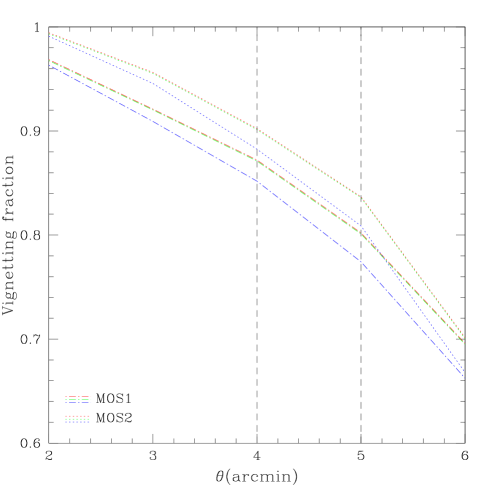
Figure 3: Vignetting expected at different off-axis angle for the two MOS detectors. The red, green, and blue lines represents the 0.7-1 keV, the 1-2 keV, and the 2-8 keV bands, respectively. The dashed black lines represents the typical off-axis angle where we would extract the background for our sample. It is clear how the background spectra could be vignetted up to a 20% factor.

Table 3: Comparison of fit results obtained with Anders & Grevesse (1989) (ANGR89) and Asplund et al. (2009) (ASPL09) solar abundance standards for four of the brightest clusters in our sample.

Cluster	Radial bin		ANGR89			ASPL09
	($r_{500}$)	$kT$(keV)	$Z(Z_{\odot})$	C-stat	$kT$(keV)	$Z(Z_{\odot})$	C-stat
RXJ2228.6+2037	0-0.15	$8.57_{-0.54}^{+0.51}$	$0.27_{-0.07}^{+0.08}$	701.9	$8.58_{-0.54}^{+0.51}$	$0.37_{-0.10}^{+0.12}$	702.4
	0.15-0.4	$7.88_{-0.47}^{+0.52}$	$0.27_{-0.06}^{+0.08}$	899.4	$7.89_{-0.47}^{+0.52}$	$0.38_{-0.11}^{+0.13}$	899.2
	0.4-0.9	$5.74_{-0.40}^{+0.44}$	$0.12\pm 0.07$	1032.4	$5.72_{-0.39}^{+0.43}$	$0.17_{-0.10}^{+0.11}$	1032.4
RXCJ1206.2-0848	0-0.15	$9.91_{-0.46}^{+0.50}$	$0.28_{-0.05}^{+0.06}$	878.2	$9.95_{-0.47}^{+0.51}$	$0.39_{-0.07}^{+0.08}$	878.5
	0.15-0.4	$11.61_{-0.65}^{+0.81}$	$0.18\pm 0.07$	1120.6	$11.61_{-0.63}^{+0.72}$	$0.26_{-0.09}^{+0.10}$	1120.6
	0.4-0.7	$9.20_{-0.83}^{+1.26}$	$0.50_{-0.14}^{+0.15}$	1109.7	$9.15_{-0.82}^{+1.19}$	$0.72\pm 0.21$	1109.1
RXJ1347.5-1145	0-0.15	$11.11\pm 0.26$	$0.34_{-0.04}^{+0.03}$	1204.2	$11.14\pm 0.26$	$0.48\pm 0.05$	1205.0
	0.15-0.4	$11.55_{-0.47}^{+0.48}$	$0.25_{-0.05}^{+0.06}$	1072.5	$11.57_{-0.46}^{+0.48}$	$0.35_{-0.07}^{+0.08}$	1073.1
	0.4-0.8	$7.74_{-0.64}^{+0.84}$	$0.15_{-0.08}^{+0.09}$	1075.3	$7.57_{-0.59}^{+0.82}$	$0.21_{-0.11}^{+0.13}$	1076.6
MS0451.6-0305	0-0.15	$9.47_{-0.57}^{+0.81}$	$0.24_{-0.08}^{+0.09}$	631.3	$9.49_{-0.57}^{+0.81}$	$0.34_{-0.12}^{+0.13}$	631.2
	0.15-0.4	$9.47_{-0.56}^{+0.67}$	$0.18\pm 0.07$	786.8	$9.46_{-0.56}^{+0.68}$	$0.25_{-0.10}^{+0.11}$	786.7
	0.4-0.7	$7.29_{-0.86}^{+1.04}$	$0.07_{-0.07}^{+0.11}$	806.2	$7.25_{-0.85}^{+1.02}$	$0.10_{-0.10}^{+0.17}$	806.3

3.3 Effects of the XMM-Newton PSF on the analysis

In contrast with Chandra, the EPIC XMM-Newton telescopes have a quite large PSF ($HEW\sim 15^{\prime\prime}$). This was a potential problem to our analysis because the emission from the cluster cores ($r<0.15r_{500}$) in principle could contaminate the spectra just outside the core ($0.15r_{500}<r<0.4r_{500}$) and viceversa, if the extraction region for the cores is similar in size to the HEW or smaller, as happens in about a third of our sample and in almost all the clusters at $z>0.7$. However, the contribution of the emission from the $0.15-0.4r_{500}$ annulus to the outer region spectra ($r>0.4r_{500}$) can be assumed to be negligible. If the source is uniform over the field, then this effect is not a major concern. However, if there are strong gradients in the emission and spectral parameters over the field (as it is the case of cooling core clusters) then the effect might be significant.

To quantify the effect of the PSF on the determination of the spectral parameters measured (and especially on the abundance measurements), we used a procedure developed in XMM-ESAS (Snowden et al. 2004) that considers the crosstalk ARFs between two contiguous regions to remove the contribution of the core from the surrounding region and viceversa. We applied it to a few clusters in the sample (RXJ1213.5, CLJ1354, MS1054.4, and CLJ1429.0) at different redshifts and core extraction radii, which shows evidence of a temperature dip at the center and abundance gradients. In all of these clusters, the differences in the temperatures measured considering the PSF correction and the temperatures measured when not considering the correction were in the range between 5% and 15%, which are comparable to or smaller than the statistical errors in the measurements. On the other hand, the differences in the abundance measures were always $\leq 0.02$ $Z_{\odot}$, i.e. well below the statistical errors. Therefore, we decided not to apply the correction to the remainder of the sample.

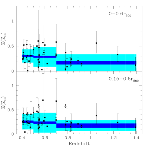
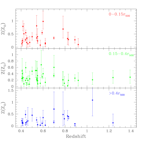
Figure 4: Left: Abundance measured by EPIC XMM-Newton as a function of the redshift for the clusters in our sample including the emission from the whole cluster at $r<0.6r_{500}$ (top) and excising the core (bottom). The error bars in $Z$ are at 1$\sigma$, while shaded areas show the weighted mean of the abundance with its error (blue) and rms dispersion (cyan) in three redshift bins. Right: Abundance measured by EPIC XMM-Newton as a function of the redshift for the clusters in our sample in different spatial bins (from top to bottom: 0-0.15$r_{500}$,0.15-0.4$r_{500}$, and $>0.4r_{500}$), with 1$\sigma$ error bars indicated.

3.4 Spectral fitting

The spectra were analyzed with XSPEC v12.5.1 (Arnaud 1996) and fitted with a single-temperature mekal model (Liedahl et al. 1995) with Galactic absorption (wabs model), in which the ratio between the elements was fixed to the solar value as in Anders & Grevesse (1989). We prefer to report metal abundances in these units of solar abundances because most of the literature still refers to them. We tested the robustness of our results to variations in the assumed emission abundance model by fitting the data for four of the brightest clusters in our sample (RXJ2228.6+2037, RXCJ1206.2-0848, RXJ1347.5-1145, and MS0451.6-0305) using also the most recent values of Asplund et al. (2009). Table 3 shows the results of the fits obtained using the two different solar abundance references. The fits were of similar quality, as can be seen from the similar values of the C-statistic, and the only significant differences were those found in the values of the fitted abundances, which we found to be consistent with a simple scaling by a factor of 1.41 (within a 3% margin), where the Asplund et al. (2009) abundances are higher than those of Anders & Grevesse (1989). This is a clear indication that we have measured the iron abundance in the ICM, as expected from the statistics we have in virtually all the cluster spectra. In addition, also the fitted temperatures using the two abundance models were all consistent.

All the spectral fits were performed over the energy range $0.7-8.0$ keV for both of the two MOS detectors. We fitted simultaneously MOS1 and MOS2 spectra to increase the quality of the statistics.

The free parameters in our spectral fits are temperature, abundance, and normalization. Local absorption is fixed to the Galactic neutral hydrogen column density, as obtained from radio data (Kalberla et al. 2005), and the redshift to the value measured from optical spectroscopy ($z$ in Table 1). We used Cash statistics applied to the source plus background, which is preferable for low S/N spectra (Nousek & Shue 1989) and requires a minimal grouping of the spectra (at least one count per spectral bin). We estimated a goodness-of-fit for the best-fit models using the XSPEC command goodness, which simulates a user-defined number of spectra based on the best-fit model itself and calculates the percentage of these simulations in which the fit statistic is smaller than that for the data. For each spectrum in the sample, we simulated 10000 spectra from the best-fit model, whose C-statistic values were compared with the value obtained from the original spectrum. For the spatially resolved bins ($r=0-0.15r_{500}$, $r=0.15-0.4r_{500}$ and $r>0.4r_{500}$), we found that the percentage of simulations with a smaller value of the C-statistic than that for the data is always less than 40%, an indication that the one-temperature model is always a good fit to the spatially resolved spectra. For the spectra extracted including emission from the whole cluster ($r=0-0.6r500$ and $r=0.15-0.6r500$), the percentage in a few cases is found to be larger than 40%, especially in the spectra with more counts. This is fully expected because the potential well of galaxy clusters is very likely to harbor a multi-temperature gas. In those cases, the one-temperature model is not a good fit to the data, but this is not a major problem because we simply wish to measure an average temperature and abundance for the integrated emission.

4 Results

The main results we attained from the spectral analysis are presented in this Section. In particular, we focus on the redshift evolution of the metal abundance considering both the integrated and spatially resolved emission from the clusters, and on the correlation of the temperature with both redshift and abundance.

4.1 Integrated abundance evolution

Although the main focus of this paper has been to spatially resolve the evolution of the abundance with redshift, a complementary measurement is an integrated measure of the abundance, which is useful when comparing with previous works in the literature.

Figure 4 (left) shows how the measured abundance in our cluster sample evolves with redshift. To perform a statistical verification of this evolution, we computed a Spearman’s rank $\rho$ for the distributions plotted in the graph considering both emission from the whole cluster ($r=0-0.6r_{500}$) and after excising the cores ($r=0.15-0.6r_{500}$). We performed 10000 Monte Carlo (MC) simulations to take into account the distribution of the errors in $Z$ in the determination of the Spearman’s rank $\rho$. In the distribution considering emission from the whole cluster, we observed a weak negative correlation between redshift and abundance with a mean Spearman’s rank $\rho=-0.12\pm 0.10$ with 39 degrees of freedom (d.o.f.), corresponding to a mean probability of no correlation $p=0.48\pm 0.32$. The negative correlation was found to be even weaker after we had excised the core, as could be deduced from the computed mean Spearman’s rank $\rho=-0.05\pm 0.11$ (again with 39 d.o.f.), which corresponds to a probability of no correlation $p=0.61\pm 0.31$. We also fitted the data points in Figure 4 (left) with a power-law such as $Z\propto(1+z)^{-\gamma}$, where $Z$ is the abundance measured and $z$ is the cluster redshift. The value of $\gamma$ (reported in Table 4) indicates a weak negative evolution with a significance lower than 2$\sigma$ in both cases. The most significant deviation from $\gamma=0$ is observed in the $0-0.6r_{500}$ sample, where $\gamma=0.75_{-0.74}^{+0.80}$ at a 90% confidence level. In the sample where the core is excised, the power-law slope is consistent with zero ($\gamma=0.61_{-0.66}^{+0.72}$).

4.2 Spatially resolved abundance evolution

As stated before, the main goal of our paper has been to study the evolution of the metal abundance in galaxy clusters through cosmic time, trying to spatially resolve the cluster emission into three radial bins. Figure 4 (right) shows how the abundance measured at different radii in the cluster sample evolves with redshift.

Similarly to the steps taken in § 4.1, we used two different statistical methods to quantify any presence of evolution: the calculation of a mean Spearman’s rank $\rho$ (averaged performing 10000 MC simulations) and a power-law fit to the data points.

In the $r<0.15r_{500}$ radial bin, we do not observe any evidence of abundance evolution with a mean Spearman’s rank $\rho=0.03\pm 0.14$ with 26 degrees of freedom (d.o.f.), corresponding to a mean probability of no correlation $p=0.62\pm 0.28$. Fitting the data points in this bin with a power-law in the form $Z\propto(1+z)^{-\gamma}$, as in § 4.1, we obtained $\gamma=-0.19_{-0.68}^{+0.72}$ (Table 4), indicating no significant evolution in agreement with the mean Spearman’s rank result.

In addition, at $0.15r_{500}<r<0.4r_{500}$, the values are very widely dispersed as is clear from the computed mean Spearman’s rank $\rho=-0.06\pm 0.12$ with 39 d.o.f., which corresponds to a probability of no correlation $p=0.54\pm 0.31$. In this case, the value of $\gamma$ from the power-law fit is positive ($\gamma=0.44_{-0.72}^{+0.78}$, as shown in Table 4), although it is consistent with zero within the 1$\sigma$ errors, confirming that no significant abundance evolution was found in this radial bin.

The correlation is not present at larger radii ($r>0.4r_{500}$) with a mean Spearman’s rank $\rho=0.08\pm 0.16$ and a mean $p=0.54\pm 0.33$. Fitting the data points with a power-law, the value of $\gamma$ is positive but also consistent with zero within $1\sigma$ in this case ($\gamma=1.65_{-1.92}^{+2.33}$, as reported in Table 4).

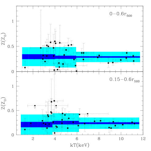
Figure 5: Temperature vs. Abundance measured for the galaxy clusters in our sample including (top) or excluding the core (bottom). The dotted lines represent the 1$\sigma$ errors in $kT$ and $Z$, while shaded areas show the weighted mean in the abundance with its error (blue) and rms dispersion (cyan) in three temperature bins. Althought the values of $Z$ show a larger spread at $kT<5$ keV, we do not find any correlation between the two quantities.

4.3 Temperature-abundance and temperature-redshift correlation

As stated in § 3.3, the PSF of EPIC could in principle have an effect on the determination of the temperature in the central two annuli of the clusters (especially at high redshift) of the order of 5-15%, if there were temperature gradients. Therefore we decided to compare the distribution of $Z$ as a function of the temperature only for the whole cluster emission (or after simply excising the core as in § 4.1).

Figure 5 shows the correlation between the temperature and the abundance measured in each cluster including ($r=0-0.6r_{500}$) and excluding the core ($r=0.15-0.6r_{500}$). Although at first glance, it appears that higher values of abundance are more frequent at low temperatures, the correlation between this two quantities is statistically very weak (as can be clearly seen from the weighted average values of $Z$ derived in three different bins of temperature).0 When we considered the emission from the whole cluster, we measured a Spearman’s rank $\rho=-0.09\pm 0.13$ with 39 d.o.f. (errors computed using 10000 MC simulations as in § 4.1), corresponding to a probability of no correlation $p=0.52\pm 0.33$. The correlation was also found to be weak after we had excised the core ($\rho=0.02\pm 0.13$ with 39 d.o.f., $p=0.56\pm 0.30$). We also fit the distribution with a power-law of the form $Z\propto kT^{-\gamma}$. The results are consistent with there being no correlation between $kT$ and $Z$ for both samples ($\gamma=-0.06\pm 0.11$ including the core, and $\gamma=-0.06\pm 0.16$ excising the core). Since, as stated before, we found that the values of $Z$ have a greater dispersion at lower temperatures, we divided each sample into two subsamples at $kT<5$ keV and $kT>5$ keV and compared them with a Kolmogorov-Smirnov (K-S) test to verify whether they come from the same distribution. Both including and excising the core, the K-S test cannot reject at a 5% confidence level the null-hypothesis that the clusters with $kT<5$ keV have the same distribution of $Z$ as the clusters with $kT>5$ keV. We therefore do not find any obvious trend in the abundance with temperature similar to those seen in other samples of galaxy clusters observed with other X-ray missions such as Chandra (BLS07) and ASCA (e.g. Baumgartner et al. 2005).

No clear correlation is also observed in the redshift versus (vs.) temperature distribution (Figure 6), as indicated by a Spearman’s rank $\rho=0.14\pm 0.11$ with 39 d.o.f., (probability of no correlation $p=0.39\pm 0.25$), for the $0-0.6r_{500}$ sample, and a Spearman’s rank $\rho=0.09\pm 0.11$ (39 d.o.f., $p=0.51\pm 0.26$) for the $0.15-0.6r_{500}$ sample. Figure 6 also shows that we have analyzed a population of clusters whose temperatures are uniformly distributed with redshift, there being no preferential redshift range containing the hottest clusters in the sample ($kT>8$ keV).

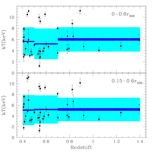
Figure 6: Redshift vs. temperature measured for the galaxy clusters in our sample including (top) or excluding the core (bottom). The errors in $kT$ are plotted at 1$\sigma$, while shaded areas show the weighted mean of the temperature with its error (blue) and rms dispersion (cyan) in three redshift bins. No clear correlation between redshift and temperature is observed.

Table 4: Values of $\gamma$ in the power-law fits of the $z$-$Z$ distribution ($Z\propto(1+z)^{-\gamma}$) in the samples present in the literature compared with those obtained in the present work. The errors in $\gamma$ and the normalization (referred at $z=0.6$) are quoted at 1$\sigma$ for one interesting parameter.

	Extraction radius	$N_{obj}$	Redshift range	$\gamma$	Norm (@$z=0.6$)
This work (§ 4.1)	$0-0.6r_{500}$	39	0.407–1.393	$0.75_{-0.45}^{+0.48}$	$0.28\pm 0.01$
	$0.15-0.6r_{500}$	39	0.407–1.393	$0.61_{-0.66}^{+0.72}$	$0.24\pm 0.02$
This work (§ 4.2)	$0-0.15r_{500}$	26	0.407–0.920	$-0.19_{-0.68}^{+0.72}$	$0.33\pm 0.02$
	$0.15-0.4r_{500}$	39	0.407–1.393	$0.44_{-0.72}^{+0.78}$	$0.23\pm 0.02$
	$>0.4r_{500}$	24	0.407–1.237	$1.65_{-1.92}^{+2.33}$	$0.13\pm 0.03$
BLS07	$0.15-0.3r_{vir}$	46	0.405–1.273	$0.68_{-0.47}^{+0.53}$	$0.28\pm 0.01$
MAU08	$0-1r_{500}$	50	0.405–1.237	$2.44_{-0.69}^{+0.76}$	$0.30\pm 0.02$
	$0.15-1r_{500}$	46	0.405–1.237	$3.87_{-0.92}^{+1.06}$	$0.22\pm 0.02$
MAU08	$0-1r_{500}$	49	0.405–1.237	$2.18_{-0.71}^{+0.77}$	$0.31\pm 0.02$
	$0.15-1r_{500}$	45	0.405–1.237	$-0.15_{-1.23}^{+1.39}$	$0.28\pm 0.02$
Anderson et al. (2009)	$0-X^{\prime\prime}$	23	0.407–1.237	$0.09_{-0.76}^{+0.88}$	$0.24\pm 0.02$

5 Discussion

The main goal of our paper has been to study the evolution of the metal abundance in galaxy clusters through cosmic time. To achieve this aim, we did not consider the emission only from the entire cluster (§ 4.1) but we also tried to spatially resolve the cluster emission into three radial bins of $0-0.15r_{500}$, $0.15-0.4r_{500}$, and $>0.4r_{500}$ (§ 4.2).

5.1 Comparison with previous works

In § 4.1, we have shown that considering the integrated emission from the whole clusters we could detect only a mild negative abundance evolution with redshift at a confidence level lower than 2$\sigma$ (as indicated by the power-law fits of the $z$-$Z$ distribution).

Notwithstanding, it is interesting to perform a quantitative comparison of our results with those obtained previously in the literature (e.g. BLS07). The Chandra samples of BLS07 and MAU08 and the XMM-Newton sample of Anderson et al. (2009) are the most suitable to perform this comparison. In these samples, we selected only the clusters at $z>0.4$ to be consistent with the redshift range probed in our work. We have 23, 46, 50, and 46 objects in this redshift range for the Anderson et al. (2009) sample, the BLS07 sample, the MAU08 sample, and the MAU08 sample with the core excised ($r<0.15r_{500}$), respectively. We performed the same power-law fit to the $z$-$Z$ relation that we used in § 4.1 for our data (in the form $Z\propto(1+z)^{-\gamma}$). The comparison of the fits with those obtained for our sample are shown in Table 4 and Figure 7, where the confidence contours on $\gamma$ and normalization (referred at z=0.6) are shown for all the datasets analyzed. From the values of $\gamma$ and normalization shown in the table and the confidence contours shown in Figure 7, it is clear how our results for the integrated measure of the abundance in the $0-0.6r_{500}$ sample (§ 4.1) are fully consistent with BLS07 sample. Both these samples do not display any significant signs of negative evolution (significance lower than 2$\sigma$). Table 4 also shows that the sample of Anderson et al. (2009) has a $\gamma\sim 0$, while the only samples showing an evolution of abundance with $z$ at a confidence level higher than 2$\sigma$ are the MAU08 Chandra samples. In particular, it is striking how the values of $\gamma$ from the MAU08 sample are significantly higher than in all the other samples (especially not considering the core emission). We note that these values are probably affected by the presence in their sample of a single cluster at high redshift with a very low upper limit measurement on $Z$ (CLJ1415.1+3612 at $z=1.030$ with $Z<0.14$ and $Z<0.04$, including and excising the core, respectively). Therefore we performed the power-law fits of their sample excluding this particular cluster to quantify its influence on the $z$ vs. $Z$ trends. While in the sample including the core, the results of the evolution strength are quite robust ($\gamma$ changes from $2.44_{-0.69}^{+0.76}$ to $2.18_{-0.71}^{+0.77}$), removing CLJ1415.1+3612 from the $0.15-1r_{500}$ sample has a dramatic effect on the measured abundance evolution. The value of $\gamma$ indeed changes from $3.87_{-0.92}^{+1.06}$, corresponding to a strong negative evolution, to $-0.15_{-1.23}^{+1.39}$, corresponding to no significant evolution. This is also evident from Figure 7, where the confidence contours in the $\gamma$-normalization parameter space referring to this sample are consistent with no evolution and with all the other datasets considered in this section. That a single deviant object could have such a strong effect on the abundance evolution significance is clearly a caveat about being careful in interpreting results based on such small samples. In any case, from the values reported in Table 4 and the projection of the contours in Figure 7, we can constrain the normalization (at $z=0.6$) to $Z\approx 0.28$ and $Z\approx 0.24$ in our $0-0.6r_{500}$ sample and in our $0.15-0.6r_{500}$ sample, respectively. These values are consistent within 1$\sigma$ with the values obtained from all the other datasets in the literature considered in the present section. We note that the lack of evolution in almost all the samples analyzed in this section could be due, at least in part, to the redshift range probed in this paper. BLS07, MAU08 and Anderson et al. (2009) did indeed detect a significant evolution in abundance, only between the low redshift clusters ($0.1\la z\la 0.3$) and the clusters at $z\gtrsim 0.5$.

As a consistency check, we also applied a Bayesian MC method to fit the datasets described above (see e.g. Andreon 2010), finding consistent results with the power-law minimum least squares fit for all the samples.

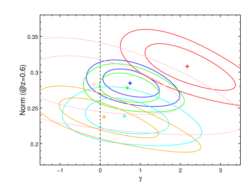
Figure 7: Confidence contours (computed at 1$\sigma$ and 2$\sigma$ for two interesting parameters) on $\gamma$ and normalization (referred to z=0.6) for all the datasets analyzed in § 5.1. Blue and cyan contours refer to our $0-0.6r_{500}$ sample and our $0.15-0.6r_{500}$ sample, respectively. The contours for MAU08 samples (computed excluding CLJ1415.1+3612, see text and Table 4) at $r=0-1r_{500}$ and $r=0.15-1r_{500}$ are plotted in red and pink, respectively. Green contours refer to the BLS07 sample, while orange contours are plotted for the Anderson et al. (2009) dataset.

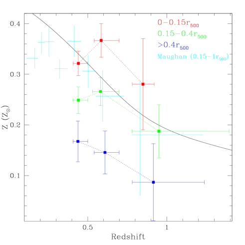
Figure 8: Mean weighted abundance in our XMM-Newton sample as a function of the redshift for the clusters in our sample in different spatial bins: 0-0.15$r_{500}$ plotted in red, 0.15-0.4$r_{500}$ in green, and $>0.4r_{500}$ in blue. The error bars represent the error in the mean and are listed in Table 5. The cyan points represent the weighted abundance measured by MAU08 for a sample of 116 clusters. The abundance values expected at different redshifts in the Ettori (2005) model are plotted as a solid black line.

Table 5: Mean weighted abundance in the three radial bins considered computed at three different redshift bins, with their errors and r.m.s. dispersions indicated.

Redshift	$\langle Z(0-0.15r_{500})\rangle\pm err\pm rms$	$\langle Z(0.15-0.4r_{500})\rangle\pm err\pm rms$	$\langle Z(>0.4r_{500})\rangle\pm err\pm rms$
0.4–0.5	$0.32\pm 0.02\pm 0.19$	$0.25\pm 0.03\pm 0.17$	$0.17\pm 0.04\pm 0.16$
0.5–0.7	$0.37\pm 0.03\pm 0.29$	$0.27\pm 0.03\pm 0.20$	$0.15\pm 0.04\pm 0.23$
0.7–1.4	$0.28\pm 0.09\pm 0.20$	$0.19\pm 0.05\pm 0.08$	$0.09\pm 0.08\pm 0.44$

5.2 Spatially resolved abundance: weighted mean and radial dependence of $Z$

In § 4.2, we resolved spatially the emission from our clusters into three radial bins. However, no evolution in abundance could be observed in each of the radial bins considered. In this case, the deviations from no evolution are even less significant than in the integrated measures we have obtained in this paper (§ 4.1) and in the results of BLS07 and MAU08. The most likely reasons for this discrepancy are the larger errors in the measure of $Z$ and the smaller sample size of the $r=0-0.15r_{500}$ and the $r>0.4r_{500}$ samples (26 and 24 clusters, respectively). Both of these reasons are clearly caused by the smaller number of counts we have when dividing the emission into three radial bins instead of considering a single spatial bin for each cluster.

Although the low quality of our statistics prevent us from any quantitative claim about the abundance evolution, it is interesting to consider a weighted mean of the abundance computed at different redshift bins to perform a qualitative comparison with the literature (in particular with MAU08) and the theoretical predictions of the Ettori (2005) model. The size of our XMM-Newton sample did not allow us to consider more than three redshift bins ($0.4<z<0.5$, $0.5<z<0.7$, and $z>0.7$) when computing the weighted mean and using as weights the statistical errors in the measure of the abundance. Figure 8 shows the mean weighted abundance in the three radial bins considered computed at the three different redshift bins listed above. The mean weighted abundances are also shown in Table 5 with their errors and r.m.s. dispersions. We have also plotted the weighted means of MAU08 for their 116 Chandra clusters (obtained by performing a stacking spectral analysis and excising the cores) and the predictions of the Ettori (2005) model for the abundance evolution in galaxy clusters. As expected, the abundance weighted-mean decreases towards larger radii (consistently with the power-law normalizations reported in Table 4). However, the $z$-$Z$ relation is consistent with no evolution at every radius. As stated before, the small number of counts in each radial bin (and the associated large errors in $Z$) for most of the clusters in the sample does not allow us to measure with sufficient accuracy the mean abundance at different redshift, and prevents any statistically significant claim about its evolution with cosmic time in the three different cluster regions considered (i.e. the core, the core surroundings, and the outskirts), in agreement to what we found in § 4.2. From Figure 8, we can see that, although there is no supporting statistical evidence of any kind of evolution, the trend in the 0.15-0.4$r_{500}$ radial bin generally complements nicely the measures of MAU08, obtained after excising the cool core ($0.15r_{500}<r<r_{500}$), and broadly agrees with the predictions of the Ettori (2005) model. In particular, the model of Ettori (2005) predicts a slope between $z=0.4$ and $z=1.4$ of $\gamma=1.7$, which is only $\sim 1.5\sigma$ above the constraints we have in our 0.15-0.4$r_{500}$ dataset.

The dependence of the abundance $Z$ on both the radius $r$ and the redshift $z$ could also be tested by fitting $Z$, $r$, and $z$ from the 89 data points in the three radial bins together (the points plotted in the right panel of Figure 4) with a function of two variables in the form

$$Z(r,z)=Z_{0}\left(1+\left(\frac{r}{r_{0}}\right)^{2}\right)^{-a}\left(\frac{1+z}{1.6}\right)^{-\gamma}.$$ (2)

In this formula, the radius of reference $r$ in each radial bin was defined as the effective radius $\bar{R}$ weighted by the emissivity distribution within a given radial bin defined by

$$S_{b}(R_{i},R_{o})=\frac{2}{(R_{o}^{2}-R_{i}^{2})}\int_{R_{i}}^{R_{o}}S_{b}\,r\,dr=S_{b}(\bar{R}),$$ (3)

where $S_{b}$ is the X-ray surface brightness, and $R_{i}$ and $R_{o}$ are the inner and outer radius of the radial bin. Under the assumption that $S_{b}\propto r^{-\alpha}$, we obtain

$$\bar{R}=\left(\frac{2}{(2-\alpha)}\times\frac{(R_{o}^{2-\alpha}-R_{i}^{2-\alpha})}{(R_{o}^{2}-R_{i}^{2})}\right)^{-1/\alpha}.$$ (4)

In our estimates, we adopt $\alpha=$ 0.7, 2.2, and 3 in the $0-0.15$, $0.15-0.4$, and $>0.4r_{500}$ radial bin, respectively, in accordance with the expected radial behaviour of the X-ray surface brightness in massive galaxy clusters (see e.g. Ettori et al. 2004). Fixing $r_{0}=0.15r_{500}$, we obtained a good fit with a $\chi^{2}\sim 107.6$ with 86 d.o.f. ($\chi_{red}^{2}\sim 1.25$). The best-fit values of the three free parameters are $Z_{0}=0.36\pm 0.03$, $a=0.32\pm 0.07$, and $\gamma=0.25\pm 0.57$. These values represent a significant negative trend of $Z$ with the radius and again no significant evolution with redshift. That the evolution with redshift is even smaller when the radial dependence is taken into account suggests that part of the claimed evidence of a negative evolution of the integrated metallicity can be ascribed to the decrease with radius in the measured abundance, for instance when the metal content is estimated in relatively smaller regions in the nearby systems.

Although the constraints on the abundance evolution with the redshift are far from being stringent, this is the first time that the abundance measured in the ICM of galaxy clusters has been parametrized as a function of both the distance from the center, and the redshift. This new result should be directly compared with the models of diffusion of metals (e.g. Ettori 2005; Loewenstein 2006; Calura et al. 2007; Cora et al. 2008) and the simulations of chemical enrichment (e.g Tornatore et al. 2004; Rebusco et al. 2005; Tornatore et al. 2007; Schindler & Diaferio 2008; Fabjan et al. 2010) in the ICM.

6 Conclusions

We have presented a spatially resolved XMM-Newton analysis of the X-ray spectra of 39 clusters of galaxies at $0.4<z<1.4$, covering a temperature range of $1.5\,\la kT\,\la 11$ keV. The main goal of this paper has been to study how the abundance evolves with redshift not only by analyzing a single emission measure performed on the whole cluster (as in e.g. BLS07; MAU08; Anderson et al. 2009), but also by spatially resolving the cluster emission in three different regions: the core region (corresponding to $0<r<0.15r_{500}$), the region immediately surrounding the core ($0.15r_{500}<r<0.4r_{500}$), and the outskirts of the cluster ($r>0.4r_{500}$). This represents the first time that a spatially resolved analysis of the metal abundance evolution through cosmic time has been attempted.

The main results of our analysis can be summarized as follows:

• Across the studied redshift range, we have not found any statistically significant abundance evolution with redshift considering the integrated emission from the whole cluster both at $r<0.6r_{500}$ and at $r=0.15-0.6r_{500}$. The most significant deviation from no evolution was found in the $0-0.6r_{500}$ sample, where a power-law fit to the $z-Z$ distribution gives a $\gamma=0.75_{-0.74}^{+0.80}$ at a 90% confidence level.

• Dividing the emission into three radial bins, we could not find any significant evidence of abundance evolution (always below $1\sigma$). The main reasons for this are probably the smaller number of counts (and the associated larger errors in $Z$) and smaller statistical samples for two of the three radial bins.

• We have not found any significant correlation between the abundance and temperature similar to that seen in other samples of galaxy clusters observed with other X-ray missions such as Chandra (BLS07) and ASCA (e.g. Baumgartner et al. 2005). Using different statistical methods (Spearman’s rank, power-law fit, K-S test), the significance of a $kT-Z$ relation is always less than $1\sigma$.

• We compared our results for the single-emission-measure abundances with previous works in the literature. Our results are fully consistent with the BLS07, MAU08, and Anderson et al. (2009) samples at $z>0.4$, as indicated by a power-law fit to the $z$-$Z$ distributions. The differences in the power-law slope $\gamma$ and in the normalizations at $z=0.6$ are always smaller than 2$\sigma$, with the largest discrepancy found when comparing with the MAU08 $0-1r_{500}$ sample.

• We found that the presence or not of a single cluster (CLJ1415.1+3612) in the MAU08 sample could dramatically change the abundance evolution measured at $z>0.4$ from a power-law fit, such that in the $0.15-1r_{500}$ sample, $\gamma$ varies from $3.87_{-0.92}^{+1.06}$ (indicating strong negative evolution) to $-0.15_{-1.23}^{+1.39}$ (no significant evolution). The impact that a single deviant object could have on the measured abundance evolution is a caveat about being careful in interpreting results based on such small samples.

• We computed error-weighted means of the spatially resolved abundances in three redshift bins: $0.4<z<0.5$, $0.5<z<0.7$, and $z>0.7$. The abundance weighted-mean is consistent with being constant with redshift at every radius, given the large 1$\sigma$ error bars. A qualitative comparison with MAU08 and the predictions of the model of Ettori (2005) shows how the trend in the error-weighted mean abundance with redshift in the 0.15-0.4$r_{500}$ radial bin complements nicely the measures of MAU08 (at $0.15r_{500}<r<r_{500}$), and broadly agrees with the predictions of Ettori (2005) model.

• We quantified the dependence of the metal abundance on both the radius $r$ and the redshift $z$ by fitting the data points available from the spatially resolved analysis with a function of two variables $Z(r,z)=Z_{0}(1+(r/0.15r_{500})^{2})^{-a}(z/0.6)^{-\gamma}$, with best-fit model values of $Z_{0}=0.36\pm 0.03$, $a=0.32\pm 0.07$, and $\gamma=0.25\pm 0.57$. This relation depicts a significant negative trend of $Z$ with the radius and, although no significant evolution with the redshift is detected, it represents the first time that the abundance measured in ICM has been parametrized as a function of both $r$ and $z$ in a way that could be directly compared with the models of diffusion of metals (e.g. Loewenstein 2006; Calura et al. 2007) and the simulations of chemical enrichment (e.g Schindler & Diaferio 2008; Fabjan et al. 2010) in the ICM.

In general, the low quality of the statistics (and large errors in $Z$) associated with most of the clusters in the sample has prevented us fron drawing any statistically significant conclusion about the different evolutionary path the abundance may have traversed through cosmic time in the three different cluster regions considered.

We stress that the results presented in this paper (from both our new analysis of the XMM-Newton exposures available at $z>0.4$ and those already presented in the literature) represent the most robust limits that could be derived from the existing XMM-Newton and Chandra archival data on the evolution of the metal content of the ICM in massive halos. Larger samples of high redshift clusters observed in the X-rays and deeper observations of the clusters already present in both Chandra and XMM-Newton archive would be crucial to place statistically significant constraints on the evolution of metal abundances in galaxy clusters and to provide a robust modelling of the physical processes responsible for the enrichment of the cluster plasma during its assembly over cosmic time.