Triangular-lattice anisotropic dimerized Heisenberg antiferromagnet:
Stability and excitations of the quantum paramagnetic phase

Abstract

Motivated by experiments on non-magnetic triangular-lattice Mott insulators, we study one candidate paramagnetic phase, the columnar dimer (or valence-bond) phase. We apply variants of the bond-operator theory to a dimerized and spatially anisotropic spin-1/2 Heisenberg model and determine its zero-temperature phase diagram and the spectrum of elementary triplet excitations (triplons). Depending on model parameters, we find that the minimum of the triplon energy is located at either a commensurate or an incommensurate wavevector. Condensation of triplons at this commensurate–incommensurate transition defines a quantum Lifshitz point, with effective dimensional reduction which possibly leads to non-trivial paramagnetic (e.g. spin-liquid) states near the closing of the triplet gap. We also discuss the two-particle decay of high-energy triplons, and we comment on the relevance of our results for the organic Mott insulator EtMe₃P[Pd(dmit)₂]₂.

I Introduction

In the search for novel phases, frustrated quantum antiferromagnets have attracted enormous attention. Here, the combined effect of geometric frustration and quantum fluctuations tends to destabilize conventional magnetic order in favor of quantum paramagnetic ground states, such as valence-bond solids (VBS) with broken lattice symmetries or featureless spin liquids.review-subir ; review-balents ; misguich

A prominent example of a frustrated quantum magnet is the spin-1/2 Heisenberg model on the triangular lattice. Although it was initially proposed by Andersonrvb-triangle that its ground state could be a resonating-valence-bond (RVB) spin liquid, it is now established that the model displays semiclassical non-collinear 120^∘ order.isotropic-model However, modifications beyond the simple nearest-neighbor exchange are believed to induce non-magnetic phases on the triangular lattice. For instance, it has been arguedschmidt10 that a combination of longer-range and multiple-spin-exchange interactions is important near the Mott transition to a metallic state, where they induce a spin-liquid state as observed in numerical studies of the triangular-lattice Hubbard model. Models with spatially anisotropic exchange interactions have been studied as well,trumper99 ; merino99 ; series-exp ; ccm ; rg ; kallin11 ; spin-liquid ; frg ; xu09 ; weichsel11 ; hauke11 interpolating from the triangular lattice to both the square-lattice and the decoupled-chain limits, and both VBS and spin-liquid phases have been proposed to occur.

Experimentally, triangular-lattice Heisenberg models are realized in a variety of materials, such as the inorganic Mott insulators Cs₂CuCl₄ and Cs₂CuBr₄ (Ref. cscucl, ; cscubr, ) and the organic compounds $\kappa$-(ET)₂Cu₂(CN)₃ (Ref. kappa-et, ) and X[Pd(dmit)₂]₂ (Refs. dmit01, ; dmit02, ; dmit03, ; dmit04, ; dmit_rev, , with X=EtMe₃Sb or EtMe₃P), all showing some degree of spatial anisotropy. In the latter two, the crystal lattice is rather soft: pressure can be used to induce an insulator-to-metal transition, with superconductivity appearing at low temperature. Spin–lattice interactions are also relevant in the insulator, as they potentially relieve frustration via dimerization. In fact, such a dimerized VBS phase has been reported for EtMe₃P[Pd(dmit)₂]₂, likely stabilized by magneto-elastic coupling.

           

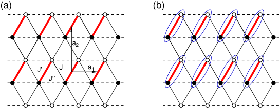
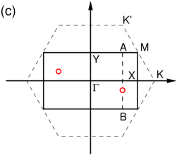
Figure 1: (Color online) (a) Lattice structure of the model (1), with exchange couplings $J$, $J^{\prime}$, and $J^{\prime\prime}$ shown as black (thin), red (thick), and dashed black lines, respectively. Solid (open) circles represent spin ${\bf S}^{1}$ (${\bf S}^{2}$) of each dimer. ${\bf a}_{1}$ and ${\bf a}_{2}$ are the primitive vectors of the dimerized lattice. (b) Dimerized ground state in the limit of large $J^{\prime}$. Here, ellipses represents a singlet. (c) Brillouin zone of the dimerized lattice (solid), together with the (hexagonal) Brillouin zone of the original triangular lattice (dashed). The open circles indicate the minimum position of $\omega_{\bf q}$ [Eq. (17)] for parameters $J^{\prime}=1.5$ and $J^{\prime\prime}=1$. Here ${\bf K}=(4\pi/3a,0)$, ${\bf K^{\prime}}=(2\pi/3a,2\pi/\sqrt{3}a)$, ${\bf X}=(\pi/a,0)$, ${\bf Y}=(0,\pi/\sqrt{3}a)$, and ${\bf M}=(\pi/a,\pi/\sqrt{3}a)$ with $a$ being the lattice spacing of the triangular lattice.

In this paper, we study the columnar dimer phase of a generic triangular-lattice antiferromagnet (AF).pattern In the absence of detailed knowledge about microscopics, we focus on a simple, yet very rich, model (Fig. 1a) with anisotropic nearest-neighbor couplings and explicit dimerization, the latter possibly arising from magneto-elastic effects. A determination of the full phase diagram of this model (see Fig. 2 for a sketch) is a hard task. Here we stick to the more modest goal of characterizing the dimer phase and its triplon excitations and locating the line of quantum phase transitions (QPTs) to a magnetically ordered state, where the triplon gap closes. To this end, we employ the bond-operator technique introduced by Sachdev and Bhatt.SachdevBhatt It turns out to be important to go beyond the linearized (i.e. non-interacting) boson problem: We discuss various approximation schemes, also providing a guideline as to which non-linear effects are important in the presence of frustration.

Among our results is the existence of a commensurate–incommensurate transition (CIT) in the excitation spectrum, i.e., the minimum of the triplon dispersion is locked at wavevector $(0,0)$ (in the coordinates of the dimerized lattice, Fig. 1) in some region of parameter space, while it moves to incommensurate momenta elsewhere. If the triplon gap closes at the CIT line, the excitations become anomalously soft, leading to a quantum Lifshitz point.qlif1 ; qlif2 We briefly discuss the unusual quantum critical regime of such a putative magnetic QPT, but also speculate about an intervening non-trivial paramagnetic phase. Finally, we discuss two-particle (as opposed to three-particle) decay of magnetic excitations,kole06 ; zhito06 which is generically possible in low-symmetry dimerized magnets.

I.1 Model

We consider a triangular-lattice Heisenberg model,

$$\mathcal{H}=\sum_{\langle i,j\rangle}J_{ij}{\bf S}_{i}\cdot{\bf S}_{j},$$ (1)

where ${\bf S}_{i}$ represents a spin–1/2 at site $i$, and the nearest-neighbor exchange couplings $J_{ij}$ equal $J$, $J^{\prime}$, and $J^{\prime\prime}$ according to the pattern shown in Fig. 1a.pattern Hereafter we employ $J=1$.

I.2 Phase diagram

To appreciate the richness of the model (1), it is useful to discuss a few limiting cases, with their properties summarized in the schematic phase diagram in Fig. 2.

(i) Line $J^{\prime\prime}=1$. On this line, for $J^{\prime}=1$, we recover the isotropic triangular-lattice AF Heisenberg model. Its ground state has non-collinear $120^{\circ}$ Néel order, with commensurate ordering wavevectors ${\bf K}=(4\pi/3a,0)$ and ${\bf K^{\prime}}=(2\pi/3a,2\pi/\sqrt{3}a)$.isotropic-model Non-collinear order can be expected to extend to small values of $J^{\prime}$. On the other hand, the limit $J^{\prime}\gg 1$ corresponds to a paramagnet of weakly coupled dimers,gia08 such that spins which are pairwise coupled by $J^{\prime}$ combine into a columnar arrangement of singlets, as illustrated in Fig. 1b.

(ii) Line $J^{\prime\prime}=0$. Model (1) is now topologically equivalent to the staggered dimerized Heisenberg model on a square lattice, recently discussed in Refs. wenzel08, ; stag-dimer, . According to quantum Monte Carlo (QMC) calculations, a order-disorder QPT takes place at $J^{\prime}_{c}=2.5196$,wenzel08 with collinear Néel order setting in for $J^{\prime}<J^{\prime}_{c}$. The line $J^{\prime\prime}=0$ also includes the square and honeycomb lattice AF at $J^{\prime}=1$ and 0, respectively.

(iii) Line $J^{\prime}=1$. Here, Eq. (1) is nothing else but the spatially anisotropic triangular-lattice AF addressed in Refs. trumper99, ; merino99, ; series-exp, ; ccm, ; rg, ; spin-liquid, ; frg, ; xu09, ; kallin11, ; weichsel11, ; hauke11, In particular, coupled-cluster calculationsccm indicate that the system displays collinear Néel order for $J^{\prime\prime}<0.8$ and non-collinear spiral order with an incommensurate ordering wavevector (except at $J^{\prime\prime}=1$) for $0.8<J^{\prime\prime}<1.8$. For $J^{\prime\prime}\gg 1$ the system consists of weakly coupled chains, and a collinear AF stateccm has been argued to arise as a result of order-from-disorder physics.rg ; kallin11 However, we note that both non-collinearweichsel11 and disordered (i.e. spin-liquid) ground statesspin-liquid ; frg have also been proposed in this regime. For $0.7<J^{\prime\prime}<0.9$ the physics is under debate as well: series-expansion studies favored a spontaneously dimerized VBS in this region,series-exp which was not found in the coupled-cluster study.ccm

In total, the phase diagram of the model (1), Fig. 2, displays a gapped paramagnetic phase, both collinear and non-collinear long-range order (LRO), as well as putative non-trivial spin-liquid regimes which may or may not be adiabatically connected to the one-dimensional limit $J^{\prime\prime}\to\infty$.

In this paper, our focus is on the properties of the dimerized paramagnet which is adiabatically connected to the limit of large $J^{\prime}$. As stated above, in a real system, such as EtMe₃P[Pd(dmit)₂]₂ the dimerization may arise spontaneously due to longer-range or ring-exchange couplings, and will then be stabilized by magneto-elastic effects. Leaving a detailed study of the latter for the future, we choose to work with explicit dimerization as in Fig. 1.pattern Most of our calculations are restricted to the parameter range $J^{\prime}>J^{\prime\prime}$ and $0\leq J^{\prime\prime}\leq 1.5$. A quantitative phase diagram obtained from various bond-operator approximations is in Fig. 3 and will be discussed in detail below.

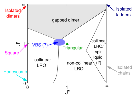
Figure 2: (Color online) Schematic phase diagram of the Heisenberg model (1), as function of the couplings $J^{\prime}$ and $J^{\prime\prime}$, keeping $J=1$. For large $J^{\prime}$, a gapped dimer phase is realized (shaded). Various other limits are indicated in the figure, see text for details. The multicritical point, where the collinear LRO, non-collinear LRO, and gapped dimer phases meet, is the quantum Lifshitz point. [The classical limit of (1) is discussed in Appendix A.]

I.3 Outline

The remainder of our paper is organized as follows: In Sec. II, we briefly summarize the bond-operator formalism that is employed to describe the paramagnetic phase of the model (1) and derive an effective Hamiltonian of interacting triplet excitations (triplons). In Sec. III, we analyze the non-interacting (i.e. harmonic) part of this Hamiltonian. We determine the magnitude and momentum-space location of the minimum energy gap of the triplons. Corrections arising from interactions – both cubic and quartic – among the triplons are analyzed in some detail in Sec. IV. For all levels of approximation, the closing of the triplon gap allows to construct the phase boundary between the singlet and long-range-ordered phases, shown in Fig. 3. In Sec. V, we discuss various aspects of our results, such as the two-particle decay of triplons due to cubic interactions, the commensurate–incommensurate transition, and the associated quantum Lifshitz point. We also comment on some implications for the organic Mott insulator EtMe₃P[Pd(dmit)₂]₂. Concluding remarks close the paper. A summary of the classical phase diagram of (1) as well as details of the calculations are relegated to the appendices.

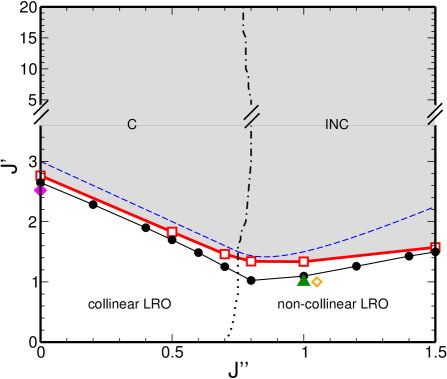
Figure 3: (Color online) Quantitative phase diagram for the Heisenberg model (1), obtained using the bond-operator formalism. The dimer phase boundary (${\color[rgb]{1,0,0}\square}$) has been obtained from the HF-cubic approximation described in the paper; for comparison we also show the results of the harmonic mean-fieldSachdevBhatt ($\CIRCLE$) and harmonic spin-wave approximations (dashed blue).kotov98 The dashed-dotted line separates the commensurate (C) and incommensurate (INC) regions of the dimer phase at large $J^{\prime}$. It continues into the dotted line which separates the phases with collinear and non-collinear LRO at small $J^{\prime}$ – note that this line is an estimate based on series-expansionseries-exp and classical-limit results (Appendix A.) Also shown are the isotropic point $J^{\prime}=J^{\prime\prime}=1$ (${\color[rgb]{0,0.8,0}\blacktriangle}$) and the point $J^{\prime}=1$, $J^{\prime\prime}=1.05$ (${\color[rgb]{0.9,0.8,0}\bf\lozenge}$) for EtMe₃P[Pd(dmit)₂]₂.dmit02 (Here, longer-range or multiple-spin interactions can be expected to be relevant in addition.) Finally, on the $J^{\prime\prime}=0$ axis we have indicated the QMC value of $J^{\prime}_{c}$ (${\color[rgb]{1,0.1,1}\blacklozenge}$) for the square-lattice staggered dimerized Heisenberg model.wenzel08

II Bond operators and triplon excitations

For $J^{\prime}>J,J^{\prime\prime}$ it is useful to view the spin pairs coupled by $J^{\prime}$ as building blocks of the model. The four states per such dimer can be efficiently represented using bond operators.SachdevBhatt which naturally lead to a description of the elementary excitations of the paramagnetic phase in terms of bosonic spin-1 modes, dubbed “triplons”.

II.1 Bond-operator representation

To introduce bond operators, the triangular lattice of spins is re-interpreted as rectangular lattice of dimers, Fig. 1b, with sites $i$. For each dimer, one introduces bosonic operators $\{s_{i}^{\dagger},t^{\dagger}_{i\alpha}\}$ ($\alpha=x,y,z$), which create the dimer states out of a fictitious vacuum. Explicitly (and omitting the site index $i$), $|s\rangle=s^{\dagger}|0\rangle$, $|\alpha\rangle=t^{\dagger}_{\alpha}|0\rangle$, where $\left|s\rangle\right.=(\left|\uparrow\downarrow\rangle\right.-\left|\downarrow\uparrow\rangle\right.)/\sqrt{2}$, $\left|x\rangle\right.=(-\left|\uparrow\uparrow\rangle\right.+\left|\downarrow\downarrow\rangle\right.)/\sqrt{2}$, $\left|y\rangle\right.=i(\left|\uparrow\uparrow\rangle\right.+\left|\downarrow\downarrow\rangle\right.)/\sqrt{2}$, $\left|z\rangle\right.=(\left|\uparrow\downarrow\rangle\right.+\left|\downarrow\uparrow\rangle\right.)/\sqrt{2}$. The Hilbert-space dimension is conserved by imposing the constraint

$$s_{i}^{\dagger}s_{i}+\sum_{\alpha}t^{\dagger}_{i\alpha}t_{i\alpha}=1$$ (2)

on every site $i$. The original spin operators ${\bf S}^{1}$ and ${\bf S}^{2}$ of each dimer are given by

$$S^{1,2}_{\alpha} = \pm\frac{1}{2}\left(s^{\dagger}t^{\phantom{\dagger}}_{\alpha}+t^{\dagger}_{\alpha}s\mp i\epsilon_{\alpha\beta\gamma}t^{\dagger}_{\beta}t^{\phantom{\dagger}}_{\gamma}\right),$$ (3)

where $\epsilon_{\alpha\beta\gamma}$ is the antisymmetric tensor with $\epsilon_{xyz}=1$ and summation convention over repeated indices is implied.

II.2 Effective theory for triplet excitations

Expressing the Hamiltonian (1) in terms of the dimer spins (${\bf S}^{1}_{i}$ and ${\bf S}^{2}_{i}$) yields

$$\mathcal{H} = \sum_{i}\left[J^{\prime}{\bf S}^{1}_{i}\cdot{\bf S}^{2}_{i}+J^{\prime\prime}\left({\bf S}^{1}_{i}\cdot{\bf S}^{1}_{i+1}+{\bf S}^{2}_{i}\cdot{\bf S}^{2}_{i+1}\right)\right]$$ (4)

$$+ J\sum_{i,n}{\bf S}^{2}_{i}\cdot{\bf S}^{1}_{i+n}.$$

Here $n=1,2,3$ corresponds to the nearest-neighbor vectors

$$\mbox{\boldmath$\tau$}_{1}=a\hat{x},\;\;\;\;\;\;\;\mbox{\boldmath$\tau$}_{2}=\sqrt{3}a\hat{y},\;\;\;\;\;\;\;\mbox{\boldmath$\tau$}_{3}=a(\hat{x}+\sqrt{3}\hat{y}),$$ (5)

with $a$ being the lattice spacing of the original triangular lattice (in the following $a=1$). Substituting Eq. (3) into (4) yields a Hamiltonian of the form

$$\mathcal{H}=\mathcal{H}_{0}+\mathcal{H}_{2}+\mathcal{H}_{3}+\mathcal{H}_{4}$$ (6)

where $\mathcal{H}_{n}$ contains $n$ triplet operators (see Appendix B for details).

In the paramagnetic phase realized for large $J^{\prime}$, the singlet can be viewed as “condensed”,SachdevBhatt formally $s^{\dagger}_{i},s_{i}\rightarrow\sqrt{N_{0}}$ in Eq. (6). As a consequence, one ends up with an effective Hamiltonian solely in terms of the (bosonic) triplet operators $t^{\dagger}_{i\,\alpha}$. In the spirit of mean-field theory, the constraint (2) is implemented on average via a Lagrange multiplier $\mu$. Both $\mu$ and $N_{0}$ will be self-consistently determined. One expects that $N_{0}\approx 1$ in the limit $J^{\prime}\gg J,J^{\prime\prime}$. (Other bond-operator schemes will be discussed in Sec. II.3 below.)

After performing a Fourier transform, i.e., $t^{\dagger}_{i\,\alpha}=N^{\prime-1/2}\sum_{\bf k}\exp(-i{\bf k}\cdot{\bf R}_{i})t^{\dagger}_{{\bf k}\alpha}$, the terms of the Hamiltonian (6) read

$$E_{0} = -3J^{\prime}N/8-\mu N(N_{0}-1)/2,$$

$$\mathcal{H}_{2} = \sum_{\bf k}\left[A_{\bf k}t^{\dagger}_{{\bf k}\alpha}t_{{\bf k}\alpha}+\frac{1}{2}B_{\bf k}\left(t^{\dagger}_{{\bf k}\alpha}t^{\dagger}_{{\bf k}\alpha}+{\rm H.c.}\right)\right],$$ (7)

$$\mathcal{H}_{3} = \frac{1}{2\sqrt{N^{\prime}}}\epsilon_{\alpha\beta\lambda}\sum_{{\bf p},{\bf k}}\xi_{{\bf k}-{\bf p}}\;t^{\dagger}_{{\bf k}-{\bf p}\alpha}t^{\dagger}_{{\bf p}\beta}t_{{\bf k}\lambda}+{\rm H.c.},$$ (8)

$$\mathcal{H}_{4} = \frac{1}{2N^{\prime}}\epsilon_{\alpha\beta\lambda}\epsilon_{\alpha\mu\nu}\sum_{{\bf q},{\bf p},{\bf k}}\gamma_{\bf k}\;t^{\dagger}_{{\bf p}+{\bf k}\beta}t^{\dagger}_{{\bf q}-{\bf k}\mu}t_{{\bf q}\nu}t_{{\bf p}\lambda}.$$ (9)

Here $N^{\prime}=N/2$, with $N$ being the number of sites of the original triangular lattice, and the momentum sum runs over the dimerized (rectangular) Brillouin zone. The coefficients $A_{\bf k}$, $B_{\bf k}$, $\xi_{\bf k}$, and $\gamma_{\bf k}$ are given by

$$A_{\bf k} = \frac{J^{\prime}}{4}-\mu+B_{\bf k},$$ (10)

$$B_{\bf k} = \frac{1}{2}N_{0}\left[(2J^{\prime\prime}-1)\cos k_{x}-\cos(\sqrt{3}k_{y})\right.$$ (11)

$$\left.\;\;\;\;\;\;\;\;\;\;\;-\cos(k_{x}+\sqrt{3}k_{y})\right],$$

$$\xi_{\bf k} = -\sqrt{N_{0}}\left[\sin k_{x}+\sin(\sqrt{3}k_{y})+\sin(k_{x}+\sqrt{3}k_{y})\right],$$

$$\gamma_{\bf k} = -\frac{1}{2}\left[(2J^{\prime\prime}+1)\cos k_{x}+\cos(\sqrt{3}k_{y})\right.$$ (13)

$$\left.\;\;\;\;\;\;\;\;\;\;\;+\cos(k_{x}+\sqrt{3}k_{y})\right].$$

A few remarks about the general structure of the effective Hamiltonian (6) are here in order: The bond-operator approach has some parallels to the Holstein-Primakoff approach to ordered magnets, with the difference that one considers fluctuations above a quantum paramagnetic state instead of a Néel state. A cubic triplet term (8) is present in many low-symmetry situations, including the model considered here and also the square-lattice staggered dimerized Heisenberg model of Refs. wenzel08, ; stag-dimer, . This is to be contrasted with spin waves where a cubic interaction term – describing two-particle decay of transverse magnons – is only present for non-collinear spin structures while it vanishes for collinear ones (see Ref. cherny09, for a discussion).

  

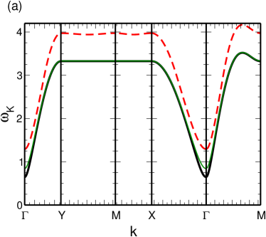
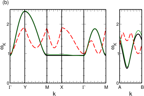
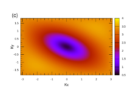
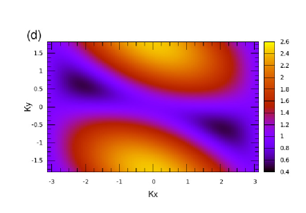
Figure 4: (Color online) Upper row: Triplon dispersion relation at the harmonic level (solid black) along paths in the dimerized Brillouin zone (Fig. 1 c), for (a) $J^{\prime}=3.0$, $J^{\prime\prime}=0$ and (b) $J^{\prime}=1.5$, $J^{\prime\prime}=1$. For comparison, the dispersion obtained within the HF approximation for the quartic term (thin green line, see Sec. IV.1) is also shown, indicating that the corrections from the quartic term are minor. Finally, the dashed red line represents the bottom of the two-particle continuum at the harmonic level. Lower row: Contour plot of the triplon energy at the harmonic level, for (c) $J^{\prime}=3.0$, $J^{\prime\prime}=0$ and (d) $J^{\prime}=1.5$, $J^{\prime\prime}=1$.

II.3 Alternative bond-operator schemes

The procedure discussed in the previous section, where the constraint (2) is included into the description via a Lagrange multiplier and $N_{0}$ is self-consistently determined, is the one originally proposed by Sachdev and Bhatt.SachdevBhatt However, alternative methods to deal with the constraint (2) can be found in the literature. Let us briefly summarize two of them.

Chubukov and Morrchubukov95 resolve the constraint via $s=(1-\lambda t^{\dagger}_{\alpha}t_{\alpha})^{1/2}$ where $\lambda$ is an artificial control parameter, with $\lambda=1$ corresponding to the physical case. The square root can now be expanded to obtain a Taylor series in the control parameter $\lambda$ – a procedure similar to the $1/S$ expansion in conventional spin-wave theory. This generates a Hamiltonian with triplon terms up to arbitrary order, which can be analyzed order by order in $\lambda$. Finally, one arrives at physical results by taking the limit $\lambda\to 1$.

Kotov et al.kotov98 instead implement the hard-core constraint explicitly in the following way. First, the $t$ operators are re-interpreted as creation operators of triplons on top of a singlet background. This is formally equivalent to setting $s_{i}^{\dagger}=s_{i}=1$. The resulting Hamiltonian contains terms up to quartic order; its harmonic piece, $\mathcal{H}_{2}$, is analogous to linear spin-wave theory. The constraint is converted into the inequality $\sum_{\alpha}t^{\dagger}_{i\alpha}t_{i\alpha}\leq 1$, which can be imposed using an infinite on-site triplet repulsion term

$$\mathcal{H}_{U}=\frac{1}{2N^{\prime}}U\sum_{i,\alpha,\beta}t^{\dagger}_{i,\alpha}t^{\dagger}_{i,\beta}t_{i,\beta}t_{i,\alpha},\;\;\;\;\;\;\;\;\;\;\;U\rightarrow\infty.$$

$\mathcal{H}_{U}$, which provides the main contribution to the renormalization of the noninteracting triplet energy, is treated using a self-consistent ladder summation of diagrams (Brueckner approximation).

Both schemes were applied to the non-frustrated square-lattice bilayer Heisenberg model, with the Brueckner approachkotov98 giving very accurate results, e.g., for the location of the phase boundary. Results of similar quality where obtained for other models with collinear spin correlations.kotov99 In contrast, we have found that the Brueckner approach is less well suited for the present triangular-lattice model: Following Ref. kotov98, , we have implemented the Brueckner approximation for the hard-core triplon repulsion and included a non-self-consistent treatment of the cubic term to second order. In the resulting phase diagram, the stability of the paramagnetic phase is clearly overestimated, i.e., we find the gapped paramagnet to be stable even at the isotropic point $J^{\prime}=J^{\prime\prime}=1$, with the critical $J^{\prime}_{c}\approx 0.75$ at $J^{\prime\prime}=1$. We suspect that the combined effect of the hard-core and cubic terms in the presence of non-collinear correlations requires a more accurate approximation, but have not explored this route further. Therefore we resort to the mean-field-based approach of Ref. SachdevBhatt, whose results are presented in the body of the paper.

             

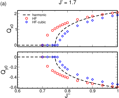
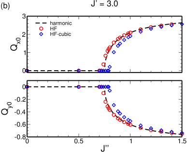
Figure 5: (Color online) $x$ and $y$ components of the momentum ${\bf Q}_{0}$ (see text for definition) as a function of $J^{\prime\prime}$ at the harmonic (dashed), HF (${\color[rgb]{1,0,0}\Circle}$), and HF-cubic (${\color[rgb]{0,0,1}\lozenge}$) approximations for the lines $J^{\prime}=1.7$ (a) and $3.0$ (b). Non-zero values of ${\bf Q}_{0}$ correspond to incommensurate correlations.

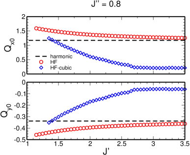
Figure 6: (Color online) $x$ and $y$ components of the momentum ${\bf Q}_{0}$ (see text for definition) as a function of $J^{\prime}$ at the harmonic (dashed), HF (${\color[rgb]{1,0,0}\Circle}$), and HF-cubic (${\color[rgb]{0,0,1}\lozenge}$) approximations for the line $J^{\prime\prime}=0.8$. In the strong-dimer limit of large $J^{\prime}$, the harmonic ${\bf Q}_{0}$ is approached for both the HF and HF-cubic results.

III Harmonic approximation

The lowest-order approximation to the triplon dynamics consists in keeping the quadratic term $\mathcal{H}_{2}$ of the Hamiltonian only, which describes the physics of noninteracting bosons. $\mathcal{H}_{2}$ can be diagonalized with the help of the Bogoliubov transformation

$$t^{\dagger}_{{\bf k}\alpha}=u_{\bf k}b^{\dagger}_{{\bf k}\alpha}-v_{\bf k}b_{-{\bf k}\alpha}.$$ (14)

One finds

$$\mathcal{H}=\bar{E}_{0}+\sum_{{\bf k}\,\alpha}\omega_{\bf k}b^{\dagger}_{{\bf k}\alpha}b_{{\bf k}\alpha},$$ (15)

where

$$\bar{E}_{0}=-\frac{3}{8}J^{\prime}NN_{0}-\frac{1}{2}\mu N(N_{0}-1)+\frac{3}{2}\sum_{\bf k}\left(\omega_{\bf k}-A_{\bf k}\right)$$ (16)

is the ground state energy,

$$\omega_{\bf k}=\sqrt{A^{2}_{\bf k}-B^{2}_{\bf k}}$$ (17)

is the energy of the triplet excitations, and the Bogoliubov coefficients in Eq. (14) obey

$$u^{2}_{\bf k},v^{2}_{\bf k}=\pm 1/2+A_{\bf k}/2\omega_{\bf k}\;\;\;\;{\rm and}\;\;\;\;u_{\bf k}v_{\bf k}=B_{\bf k}/2\omega_{\bf k}.$$ (18)

From the saddle points conditions $\partial E_{0}/\partial N_{0}=0$ and $\partial E_{0}/\partial\mu=0$, self-consistent equations for $\mu$ and $N_{0}$ follow (see Appendix C for details)

$$\mu = -\frac{3J^{\prime}}{4}+\frac{3}{N_{0}}\sum_{\bf k}B_{\bf k}v_{\bf k}\left(v_{\bf k}-u_{\bf k}\right),$$ (19)

$$N_{0} = 1-\frac{3}{N^{\prime}}\sum_{\bf k}v^{2}_{\bf k}=1-\frac{1}{N^{\prime}}\sum_{{\bf k}\,\alpha}\langle t^{\dagger}_{{\bf k}\alpha}t_{{\bf k}\alpha}\rangle.$$ (20)

Once $\mu$ and $N_{0}$ are known, the triplon energy (17) is completely determined.

In Fig. 4, we show the triplon dispersion relation for two sets of model parameters inside the disordered phase. For the case $J^{\prime}=3$ and $J^{\prime\prime}=0$, the minimum gap is located at ${\bf\Gamma}$, the center of the dimerized Brillouin zone, while for $J^{\prime}=1.5$ and $J^{\prime\prime}=1.0$, the minimum gap is at incommensurate momenta, ${\bf Q}_{0}=\pm(2\pi/3,-\pi/3\sqrt{3})$. Indeed, within the harmonic approximation, the momentum ${\bf Q}_{0}$ associated with the triplon gap can be analytically calculated. From the solution of $\nabla_{\bf q}\omega_{\bf q}=\nabla_{\bf q}B_{\bf q}=0$, one finds that it depends only on the coupling $J^{\prime\prime}$, namely

$${\bf Q}_{0}=\left\{\begin{array}[]{cc}(0,0),&0\leq J^{\prime\prime}\leq 0.75,\\ \pm({q_{\rm xm}},{q_{\rm ym}}),&J^{\prime\prime}>0.75,\end{array}\right.$$ (21)

with

$${q_{\rm xm}} = 2\arccos\left(\frac{1}{4J^{\prime\prime}-2}\right),$$

$${q_{\rm ym}} = -\frac{1}{\sqrt{3}}\arccos\left(\frac{1}{4J^{\prime\prime}-2}\right).$$ (22)

Note that ${\bf Q}_{0}$ continuously moves from a commensurate, $(0,0)$, to an incommensurate point, $\pm(q_{\rm xm},q_{\rm ym})$, as $J^{\prime\prime}$ increases, defining a commensurate-incommensurate transition (CIT) in the excitation spectrum at $J^{\prime\prime}_{\rm CIT}=0.75$, see Fig. 5. At the present harmonic level, ${\bf Q}_{0}$ only depends on $J^{\prime\prime}$, but this does not hold once corrections are included, see Sec. IV. Further aspects of the CIT will be discussed in Sec. V.2 below.

Parenthetically, we note that – at the harmonic level – one recovers the spin-wave-type approximation of Kotov et al.kotov98 (see Sec. II.3) if, instead of calculating $\mu$ and $N_{0}$ self-consistently, one sets $\mu=-3J^{\prime}/4$ and $N_{0}=1$.

IV Triplon interactions

Both the cubic and quartic interaction terms, $\mathcal{H}_{3}$ (8) and $\mathcal{H}_{4}$ (9), renormalize the triplon energy and, consequently, shift the phase boundary of the paramagnetic phase. Moreover, the cubic term also induces two-particle decay of triplons as discussed in Refs. kole06, ; zhito06, .

In order to include triplon-triplon interactions into our description, we treat the effect of $\mathcal{H}_{4}$ at the mean-field level (Sec. IV.1) and the one of $\mathcal{H}_{3}$ perturbatively (Sec. IV.2).

Figure 7: (Color online) Parameter $N_{0}$ as a function of $J^{\prime}$ for the lines $J^{\prime\prime}=0$ and $J^{\prime\prime}=1$ at the harmonic and Hartree-Fock levels.

IV.1 Hartree-Fock approximation

We treat the quartic triplon interaction within the self-consistent Hartree-Fock (HF) approximation. It is straightforward to show that Eq. (9) assumes the form (for details see Appendix A of Ref. cherny09, )

$$\mathcal{H}^{\rm HF}_{4}=E^{\rm HF}_{0}+\sum_{\bf k}\left[A^{\rm HF}_{\bf k}t^{\dagger}_{{\bf k}\alpha}t_{{\bf k}\alpha}+\frac{1}{2}B^{\rm HF}_{\bf k}\left(t^{\dagger}_{{\bf k}\alpha}t^{\dagger}_{{\bf k}\alpha}+{\rm H.c.}\right)\right].$$ (23)

Here

$$E^{\rm HF}_{0} = \frac{3}{N^{\prime}}\sum_{{\bf k}\,{\bf q}}\gamma_{\bf k}\left(\bar{v}^{2}_{{\bf k}+{\bf q}}\bar{v}^{2}_{\bf q}-\bar{v}_{{\bf k}+{\bf q}}\bar{u}_{{\bf k}+{\bf q}}\bar{v}_{\bf q}\bar{u}_{\bf q}\right),$$

$$A^{\rm HF}_{\bf k} = -\frac{2}{N^{\prime}}\sum_{\bf q}\,\gamma_{{\bf q}-{\bf k}}\bar{v}^{2}_{\bf q}\;=\sum_{n=1}^{3}A^{\rm HF}_{n}\cos({\bf k}\cdot\mbox{\boldmath$\tau$}_{n}),$$

$$B^{\rm HF}_{\bf k} = -\frac{2}{N^{\prime}}\sum_{\bf q}\,\gamma_{{\bf q}-{\bf k}}\bar{u}_{\bf q}\bar{v}_{\bf q}=\sum_{n=1}^{3}B^{\rm HF}_{n}\cos({\bf k}\cdot\mbox{\boldmath$\tau$}_{n}),$$

with $\gamma_{\bf k}$ being the bare quartic vertex (13), $\bar{u}_{\bf q}$ and $\bar{v}_{\bf q}$ the Bogoliubov coefficients (see definition below), $\mbox{\boldmath$\tau$}_{n}$ the nearest-neighbor vectors (5), and the coefficients $A^{\rm HF}_{n}$ read

$$A^{\rm HF}_{1} = (J^{\prime\prime}+2)\frac{1}{N^{\prime}}\sum_{\bf k}\cos(k_{x})\bar{u}^{2}_{\bf k},$$

$$A^{\rm HF}_{2} = \frac{1}{N^{\prime}}\sum_{\bf k}\cos(\sqrt{3}k_{y})\bar{u}^{2}_{\bf k},$$ (25)

$$A^{\rm HF}_{3} = \frac{1}{N^{\prime}}\sum_{\bf k}\cos(k_{x}+\sqrt{3}k_{y})\bar{u}^{2}_{\bf k}.$$

Similar expressions hold for $B^{\rm HF}_{n}$ but with $\bar{u}^{2}_{\bf k}\rightarrow\bar{u}_{\bf k}\bar{v}_{\bf k}$.

The final Hamiltonian is now given by $\mathcal{H}=E_{0}+E^{\rm HF}_{0}+\mathcal{H}_{2}+\mathcal{H}^{\rm HF}_{4}$. It is quadratic in triplet operators and can also be diagonalized by the Bogoliubov transformation (14), namely

$$\mathcal{H}=\bar{E}^{\rm HF}_{0}+\sum_{{\bf k}\,\alpha}\bar{\omega}_{\bf k}b^{\dagger}_{{\bf k}\alpha}b_{{\bf k}\alpha}.$$ (26)

In the above expression, the renormalized triplon energy $\bar{\omega}_{\bf k}$ is equal to Eq. (17) but now $A_{\bf k}\rightarrow\bar{A}_{\bf k}=A_{\bf k}+A^{\rm HF}_{\bf k}$ and $B_{\bf k}\rightarrow\bar{B}_{\bf k}=B_{\bf k}+B^{\rm HF}_{\bf k}$. The ground state energy $\bar{E}^{\rm HF}_{0}$ is similar to Eq. (16) apart from the replacements $\omega_{\bf k}\rightarrow\bar{\omega}_{\bf k}$ and $A_{\bf k}\rightarrow\bar{A}_{\bf k}$ and the inclusion of $E^{\rm HF}_{0}$. Finally, the Bogoliubov coefficients and the analog of the self-consistent equations (19) and (20) now read

$$\bar{u}^{2}_{\bf k},\bar{v}^{2}_{\bf k} = \pm 1/2+\bar{A}_{\bf k}/2\bar{\omega}_{\bf k},\;\;\;\;\;\bar{u}_{\bf k}\bar{v}_{\bf k}=\bar{B}_{\bf k}/2\bar{\omega}_{\bf k},$$ (27)

$$\mu = -\frac{3J^{\prime}}{4}+\frac{3}{N_{0}}\sum_{\bf k}B_{\bf k}\bar{v}_{\bf k}\left(\bar{v}_{\bf k}-\bar{u}_{\bf k}\right),$$ (28)

$$N_{0} = 1-\frac{3}{N^{\prime}}\sum_{\bf k}\bar{v}^{2}_{\bf k}.$$ (29)

Note that $B_{\bf k}$ (not $\bar{B}_{\bf k}$) enters the momentum summation in Eq. (28) (for details, see Appendix C). In addition to $\mu$ and $N_{0}$, now $A^{\rm HF}_{1,2,3}$ and $B^{\rm HF}_{1,2,3}$ are also self-consistently calculated. The set of equations (23)–(29) constitutes HF approximation.

The resulting triplon dispersion is included in Fig. 4, which shows that corrections arising from $\mathcal{H}^{\rm HF}_{4}$ are small, except for a slight upward renormalization of the gap. For a fixed $J^{\prime}$, the minimum wavevector ${\bf Q}_{0}$ displays the same qualitative behavior in terms of $J^{\prime\prime}$ as found in the harmonic approximation, see Fig. 5. In the incommensurate regime, ${\bf Q}_{0}$ numerically deviates from the harmonic result for small $J^{\prime}$ (but recovers the harmonic results in the large-$J^{\prime}$ limit), see Fig. 6. Moreover, the line marking the CIT is slightly shifted as well, see Fig. 5.

Fig. 7 shows the evolution of $N_{0}$ as a function of $J^{\prime}$ for fixed $J^{\prime\prime}$, again comparing the HF results to those from the harmonic approximation. The deviations are small in general and vanish in the strong-dimer limit $J^{\prime}\to\infty$. Inside the disordered phase, we observe $N_{0}>0.7$ which implies that $v_{\bf k}$ and $\bar{v}_{\bf k}\lesssim 0.1$, see Eqs. (20) and (29). The fact that $\bar{v}_{\bf k}$ is a small quantity is used in order to derive the self-consistent equations (28) and (29), see Appendix C for details.

We note that we experienced more difficulties in obtaining self-consistent solutions near the phase boundary in the HF approximation as compared to the harmonic one, but these problems are cured upon including the cubic term, see Sec. IV.2 below.

Figure 8: (a) Renormalized cubic vertices $\Gamma_{1}({\bf k},{\bf p})$, (1), and $\Gamma_{2}({\bf k},{\bf p})$, (2). Here $(\alpha,\beta,\gamma)$ = $(x,y,z)$, $(z,x,y)$, and $(y,z,x)$. (b)–(e) Lowest-order diagrams resulting from the combination of vertices (1) and (2) which contribute to the normal self-energy $\Sigma_{3}({\bf k},\omega)$.

IV.2 Hartree-Fock-cubic approximation

We implement a Hartree-Fock-cubic (HF-cubic) approximation by perturbatively adding the effect of $\mathcal{H}_{3}$ to the mean-field Hamiltonian $\mathcal{H}=E_{0}+E^{\rm HF}_{0}+\mathcal{H}_{2}+\mathcal{H}^{\rm HF}_{4}$. This scheme, which considerably simplifies the treatment of the cubic triplet interaction, is similar in spirit to the one adopted in Refs. kotov98, ; kotov99b, , where an interacting Hamiltonian for triplets without the cubic term is treated self-consistently first, and then the lowest-order corrections due to the cubic term are added.

     

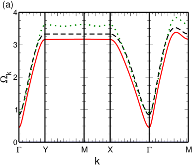
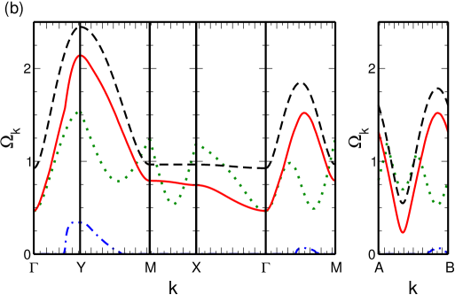
Figure 9: (Color online) Triplon dispersion relation along some particular lines of the dimerized Brillouin zone for (a) $J^{\prime}=3$ and $J^{\prime\prime}=0$ and (b) $J^{\prime}=1.5$ and $J^{\prime\prime}=1$ at the HF (dashed black line) and HF-cubic (solid red line) approximations. The triplon decay rate $\tilde{\Gamma}_{\bf k}$ (dot-dashed blue line) and the bottom of the two-particle continuum (dotted green line) both at the HF-cubic approximation are also shown. The A–B line includes the triplon minimum energy of the corresponding approximation.

Using the Bogoliubov transformation (14) with the renormalized coefficients $\bar{u}_{\bf k}$ and $\bar{v}_{\bf k}$ (27), one can show that $\mathcal{H}_{3}$ (8) in terms of the $b^{\dagger}_{{\bf k}\alpha}$ and $b_{{\bf k}\alpha}$ operators reads

$$\mathcal{H}_{3} = \frac{1}{2\sqrt{N^{\prime}}}\sum_{{\bf k},{\bf p}}\sideset{}{{}^{\prime}}{\sum}_{\alpha,\beta,\gamma}\Gamma_{1}({\bf k},{\bf p})(b^{\dagger}_{{\bf k}-{\bf p}\alpha}b^{\dagger}_{{\bf p}\beta}b_{{\bf k}\gamma}+{\rm H.c.})$$ (30)

$$+ \frac{1}{2\sqrt{N^{\prime}}}\sum_{{\bf k},{\bf p}}\Gamma_{2}({\bf k},{\bf p})(b^{\dagger}_{{\bf k}-{\bf p}x}b^{\dagger}_{{\bf p}y}b^{\dagger}_{-{\bf k}z}+{\rm H.c.}).$$

Here the sum over $\alpha,\beta,\gamma$ has only three components: $(\alpha,\beta,\gamma)=(x,y,z)$, $(z,x,y)$, and $(y,z,x)$. The renormalized vertex $\Gamma_{1}({\bf k},{\bf p})$ is given by

$$\Gamma_{1}({\bf k},{\bf p}) = \left(\xi_{{\bf k}-{\bf p}}-\xi_{\bf p}\right)\left(\bar{u}_{{\bf k}-{\bf p}}\bar{u}_{\bf p}\bar{u}_{\bf k}+\bar{v}_{{\bf k}-{\bf p}}\bar{v}_{\bf p}\bar{v}_{\bf k}\right)$$ (31)

$$+ \left(\xi_{\bf k}+\xi_{\bf p}\right)\left(\bar{v}_{{\bf k}-{\bf p}}\bar{u}_{\bf p}\bar{v}_{\bf k}+\bar{u}_{{\bf k}-{\bf p}}\bar{v}_{\bf p}\bar{u}_{\bf k}\right)$$

$$- \left(\xi_{{\bf k}-{\bf p}}+\xi_{\bf k}\right)\left(\bar{v}_{{\bf k}-{\bf p}}\bar{u}_{\bf p}\bar{u}_{\bf k}+\bar{u}_{{\bf k}-{\bf p}}\bar{v}_{\bf p}\bar{v}_{\bf k}\right),\;\;\;\;$$

with $\xi_{\bf p}$ being the bare cubic vertex (LABEL:xi), and the vertex $\Gamma_{2}({\bf k},{\bf p})=-\Gamma_{1}({\bf k},{\bf p})$ in addition to the replacements $\bar{u}_{\bf k}\leftrightarrow\bar{v}_{\bf k}$. The vertices $\Gamma_{1}({\bf k},{\bf p})$ and $\Gamma_{2}({\bf k},{\bf p})$ are illustrated in Fig. 8a.

The lowest-order diagrams which contribute to the (normal) self-energy $\Sigma_{3}({\bf k},\omega)$ are shown in Figs. 8(b)–(e). In each diagram, the solid line corresponds to the bare $b$ triplon propagator (we now omit the index $\alpha$ since the three triplon branches are degenerate)

$$G^{-1}_{0}({\bf k},\omega)=\omega-\bar{\omega}_{\bf k}+i\delta.$$ (32)

Note here that no anomalous bare $b$ propagators exist; in principle, those are generated in perturbation theory, but will be neglected in the following.comment01 Using standard diagrammatic techniques for bosons at zero temperature, one shows that only the diagrams (b) and (e) are finite, and therefore $\Sigma_{3}({\bf k},\omega)=\Sigma^{(b)}_{3}({\bf k},\omega)+\Sigma^{(e)}_{3}({\bf k},\omega)$ with

$$\Sigma^{(b)}_{3}({\bf k},\omega) = \frac{1}{4N^{\prime}}\sum_{\bf q}\frac{\Gamma^{2}_{1}({\bf k},{\bf q})}{\omega-\bar{\omega}_{\bf q}-\bar{\omega}_{{\bf k}-{\bf q}}+i\delta},$$

$$\Sigma^{(e)}_{3}({\bf k},\omega) = -\frac{1}{4N^{\prime}}\sum_{\bf q}\frac{\Gamma^{2}_{2}({\bf k},{\bf q})}{\omega+\bar{\omega}_{\bf q}+\bar{\omega}_{{\bf k}-{\bf q}}-i\delta}.$$ (33)

The renormalized triplon energy $\Omega_{\bf k}$ is given by the poles of the full Green’s function $G({\bf k},\omega)$, i.e,

$$G^{-1}({\bf k},\omega)=\omega-\bar{\omega}_{\bf k}-\Sigma_{3}({\bf k},\omega)=0.$$ (34)

We solve Eq. (34) within the so-called off-shell approximation, which consists in evaluating the self-energy at $\omega=\Omega_{\bf k}-i\tilde{\Gamma}_{\bf k}$, i.e.

$$\Omega_{\bf k}-i\tilde{\Gamma}_{\bf k}-\bar{\omega}_{\bf k}-\Sigma_{3}({\bf k},\Omega_{\bf k}-i\tilde{\Gamma}_{\bf k})=0.$$ (35)

[Recall that in the more common on-shell approximation, the self-energy is evaluated at the bare single-particle energy, i.e., $\Omega_{\bf k}-i\tilde{\Gamma}_{\bf k}-\bar{\omega}_{\bf k}-\Sigma_{3}({\bf k},\bar{\omega}_{\bf k})=0.$] Moreover, instead of using Eq. (35), causality requires to consider

$$\Omega_{\bf k}-i\tilde{\Gamma}_{\bf k}-\bar{\omega}_{\bf k}-\Sigma_{3}({\bf k},\Omega_{\bf k}+i\tilde{\Gamma}_{\bf k})=0.$$ (36)

The procedure outlined above follows Ref. cherny09, where spin-wave excitations of the isotropic triangular-lattice AF Heisenberg model ($J^{\prime}=J^{\prime\prime}=1$) were calculated. It is shown by Chernyshev et al.cherny09 that the on-shell approximation leads to discontinuities in the spin-wave spectrum and concomitant logarithmic singularities in the decay rate $\tilde{\Gamma}_{\bf k}$, and that the off-shell approximation regularizes such singularities. Finally, the replacement $\Omega_{\bf k}-i\tilde{\Gamma}_{\bf k}\rightarrow\Omega_{\bf k}+i\tilde{\Gamma}_{\bf k}$ in the argument of the self-energy guarantees that the quasiparticle pole is in the correct half of the complex plane (we refer the reader to the Appendix D, Ref. cherny09, , for details).

In Fig. 9, we compare the renormalized triplon energy $\Omega_{\bf k}$ obtained in the HF–cubic approximation to that from HF. Clearly, the inclusion of the cubic term leads to sizeable changes of the dispersion, which are particularly pronounced in the incommensurate regime [see Fig. 9 b for $J^{\prime}=1.5$ and $J^{\prime\prime}=1$]. For instance, the dispersion along ${\bf\Gamma}-{\bf M}$ is significantly enhanced by the cubic term. Most notably, the triplon gap $\Delta$ is renormalized downwards, see Fig. 10 below. In other words, cubic interactions tend to destabilize the paramagnetic phase, whereas (repulsive) quartic interactions have the opposite effect.

The behavior of the minimum wavevector ${\bf Q}_{0}$ as a function of $J^{\prime\prime}$ is again qualitatively similar to the harmonic one, Fig. 5. Interestingly, the shift of the CIT line due to the cubic interaction is opposite (and larger) to that induced by the quartic interaction, such that the CIT line is now located at some $J^{\prime\prime}_{\rm CIT}>0.75$ which moreover depends non-monotonically on $J^{\prime}$, Fig. 3.

Fig. 9 also displays the decay rate of triplons caused by two-particle decay via $\mathcal{H}_{3}$ — this is non-zero whenever the single-particle branch is above the two-particle threshold.

We conclude that the cubic triplon term is of vital importance for a quantitative description of the triplon dynamics in the frustrated coupled-dimer model (1), especially in the incommensurate regime. This is in contrast to, e.g., the unfrustrated asymmetric bilayer model studied in Ref. kotov98, where the cubic term leads to minor corrections only. A further discussion of physical implications of our results is given below.

V Discussion

V.1 Phase boundary

For the different levels of approximation, the evolution of the energy gap $\Delta$ with the dimerization strength $J^{\prime}$ is shown in Fig. 10 for $J^{\prime\prime}=0$, $0.8$, and $1$. As expected, $\Delta$ increases with $J^{\prime}$; the vanishing of the gap defines a critical value $J^{\prime}_{c}$ where the singlet phase becomes unstable towards magnetic order. Assuming a continuous QPT, we fit the data to

$$\Delta=a_{0}+a_{1}J^{\prime}+a_{2}\frac{1}{J^{\prime}}+a_{3}(J^{\prime})^{2},$$ (37)

and use the condition $\Delta=0$ to estimate the critical coupling $J^{\prime}_{c}$. (Note that the present approximations cannot be expected to yield non-trivial critical exponents. Omitting the $1/J^{\prime}$ fitting term leads to only minor changes of $J^{\prime}_{c}$. )

     

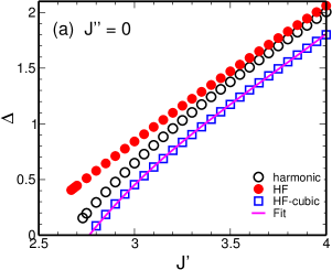
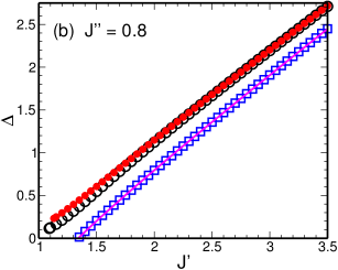
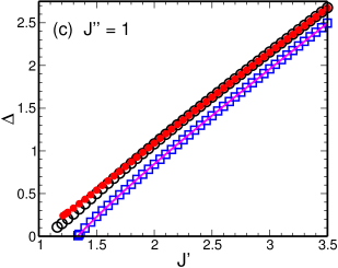
Figure 10: (Color online) Triplon gap $\Delta$ as a function of $J^{\prime}$ for (a) $J^{\prime\prime}=0$, (b) $J^{\prime\prime}=0.8$, and (c) $J^{\prime\prime}=1$ at the harmonic ($\Circle$), HF (${\color[rgb]{1,0,0}\CIRCLE}$), and HF-cubic (${\color[rgb]{0,0,1}\square}$) approximations. The solid line is a fit to the data using Eq. (37).

The resulting phase boundary for $0<J^{\prime\prime}<1.5$ is shown in Fig. 3, with the HF-cubic result (${\color[rgb]{1,0,0}\square}$) being our best approximation. The phase diagram in Fig. 3 displays four distinct regions: At large $J^{\prime}$ we have the gapped dimer phase, with spin correlations peaked at ${\bf Q}_{0}=(0,0)$ for $0\leq J^{\prime\prime}\leq J^{\prime\prime}_{\rm CIT}$ and incommensurate ${\bf Q}_{0}$ for $J^{\prime\prime}>J^{\prime\prime}_{\rm CIT}$. At the harmonic level $J^{\prime\prime}_{\rm CIT}$ equals $0.75$, but acquires a $J^{\prime}$ dependence from anharmonic terms, see Figs. 5 and 6. The closing of the triplon gap at $J^{\prime}_{c}$ for a given $J^{\prime\prime}$ leads to magnetic long-range order at wavevector ${\bf Q}_{0}$ (provided that no other phase intervenes). One concludes that the system displays collinear Néel order for $J<J^{\prime\prime}_{\rm CIT}$ and non-collinear spiral order for $J^{\prime\prime}>J^{\prime\prime}_{\rm CIT}$. As indicated in Fig. 2, an additional paramagnetic phase might be realized near the crossing of the CIT and the order-disorder transition lines,series-exp with a more detailed discussion given in Sec. V.2.

Let us quantitatively discuss the evolution for two values of $J^{\prime\prime}$. (i) $J^{\prime\prime}=0$: Here we find a critical coupling $J^{\prime}_{c}=2.65$ ($2.76$) at the harmonic (HF-cubic) level, which is quite close to the one determined via QMC simulations for the (topologically equivalent) staggered dimerized AF Heisenberg model on a square lattice, ${J^{\prime}}_{c}^{\rm QMC}=2.5196$.wenzel08 For $J^{\prime}<J^{\prime}_{c}$ the system indeed develops collinear Néel order with ${\bf Q}_{0}=(0,0)$.wenzel08 ; stag-dimer (ii) $J^{\prime\prime}=1$, where we find $J^{\prime}_{c}=1.09$ ($1.34$) at the harmonic (HF-cubic) level. Again, this is a very reasonable result since LRO is certainly present at the isotropic point ($J^{\prime}=J^{\prime\prime}=1$). One difference to case (i) is that the ordering wavevector varies with $J^{\prime}$ inside the ordered phase (see appendix A for the corresponding classical-limit results); therefore, ${\bf Q}_{0}$ at the phase boundary is distinct from the Goldstone wavevectors ${\bf K},{\bf K^{\prime}}$ of the $120^{\circ}$ structure, see also Fig. 1c.

V.2 Commensurate–incommensurate transition

As shown above, the minimum wavevector ${\bf Q}_{0}$ of the triplon dispersion in the gapped paramagnetic phase of the Heisenberg model (1) is locked to $(0,0)$ for small $J^{\prime\prime}$, while it moves to incommensurate values for larger $J^{\prime\prime}$ (Figs. 5 and 6), with the boundary being located near $J^{\prime\prime}_{\rm CIT}\lesssim 0.75$. This commensurate-incommensurate transition (CIT), driven by increasing magnetic frustration, has various consequences.

Right at the CIT, the quadratic piece of the triplon dispersion vanishes in one of the two space directions (independent of the level of approximation), i.e., we find for the triplon propagator

$$G^{-1}({\bf k},\omega)=-\omega^{2}+\Delta^{2}+c_{1}\tilde{k}_{1}^{2}+d_{1}\tilde{k}_{2}^{4}$$ (38)

in a small-momentum expansion around the ${\bf\Gamma}$ point, where $\tilde{k}_{1,2}$ are the two components of ${\bf k}$ perpendicular and parallel to the ${\bf Q}_{0}$ which is taken beyond the CIT. Moreover, in the incommensurate regime near the CIT the dispersion along the $\tilde{k}_{2}$ direction (connecting ${\bf\Gamma}$ and ${\bf Q}_{0}$) is anomalously flat. This is illustrated in Fig. 11, which shows a contour plot of the triplon dispersion $\Omega_{\bf k}$ (HF-cubic approximation) for $J^{\prime}=1.5$ and $J^{\prime\prime}=0.8$. Qualitatively, the soft dispersion near the CIT will lead to an effective dimensional reduction. When the triplon gap closes, $\Delta=0$, Eq. (38) defines a quantum Lifshitz point, see Sec. V.4 below.

Of course, the physics underlying the CIT is also observed inside the ordered phase. This has been studied in particular in the non-dimerized case, $J^{\prime}=1$. Linear spin-wave theorytrumper99 ; merino99 yields a QPT from collinear Néel to spiral order at $J^{\prime\prime}_{c}=0.5$, where the ordering wavevector changes from a commensurate to an incommensurate value. (The analysis of the classical ground state for the general case $J^{\prime}\neq 1$ is given in Appendix A.) The magnetization curve has a minimum at the transition, where the spin-wave velocity vanishes along one particular direction in $k$ space. Coupled-cluster calculationsccm find a scenario similar to spin-wave theory, but here $J^{\prime\prime}_{c}\approx 0.8$. Finally, series expansion resultsseries-exp not only indicate a CIT at $J^{\prime\prime}\approx 0.75$, but they also provide evidence for a disordered phase in the vicinity of the CIT, i.e, for $0.68<J^{\prime\prime}<0.91$.

V.3 Two-particle decay

The cubic triplon term $\mathcal{H}_{3}$ is generically present in the model (1) and thus enables two-particle decay of triplons.kole06 ; zhito06 Such decay occurs if the one-triplon dispersion moves inside the two-particle continuum.

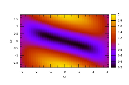
Figure 11: (Color online) Contour plot of the triplon energy $\Omega_{\bf k}$ (HF-cubic), for $J^{\prime}=1.5$ and $J^{\prime\prime}=0.8$, i.e., near the CIT.

As can be seen from Fig. 9, two-particle decay does not happen in the commensurate regime of small $J^{\prime\prime}$, where one-particle spectrum is always below the two-particle continuum. Note that an exceptional case is realized right at the QPT to the magnetically ordered state, where the lower bound of the two-particle continuum coincides with the single-particle branch near the ordering wavevector $(0,0)$. This non-trivial coupling has been argued to lead to a novel universality class for the phase transition,stag-dimer see also Sec. V.4 below.

The situation is different in the incommensurate regime, where high-energy triplons can decay into triplon pairs, see Fig. 9 for the calculated decay rate. Note that such decay never happens near ${\bf Q}_{0}$, i.e., cubic interactions are not part of the critical theory in the incommensurate case.

As an aside, we note that decay of high-energy modes also occurs inside the ordered phase, where spin waves can decay into pairs of spin waves provided that the order is non-collinear, for details see Ref. cherny09, .

V.4 Quantum criticality

Let us briefly discuss the quantum phase transitions in the phase diagram shown in Fig. 2.

The transition from the dimer phase to the collinear LRO state with ${\bf Q}_{0}=(0,0)$ would in principle be expected to be in the standard Heisenberg [or O(3)] universality class in $D=2+1$ dimensions; however, the cubic triplon term becomes part of the critical theory and leads to a new universality class (labelled class B in Ref. stag-dimer, ), with leading O(3) exponents and anomalously large corrections to scaling.wenzel08 ; stag-dimer

The transition from the dimer phase to the non-collinear LRO state does not display this complication and therefore is a standard O($N$) QPT in $D=2+1$, with $N=4$ (assuming a single transition to coplanar spiral order).

Finally, we can discuss the multicritical point where the collinear LRO, non-collinear LRO, and dimer phases meet. Here, the softness of the triplon dispersion in one direction, Eq. (38), implies that the quadratic piece of the critical field theory takes the form

$$\mathcal{S}=\int d^{2}xd\tau\,\phi_{a}(\delta+\partial_{\tau}^{2}+\partial_{x}^{2}+\partial_{y}^{4})\phi_{a}$$ (39)

where $\phi_{a}$ are the components of the magnetic order parameter, and $\delta=0$ defines the phase transition point. Such $(d,m)$ quantum Lifshitz points (here $d=2$, and $m=1$ refers to the number of “soft” directions) have been discussed before,qlif1 ; qlif2 but the relevant case of $d=2$ dimensions with undamped order-parameter dynamics has not been studied in any detail. A thorough analysis of this critical theory is therefore deferred to a future publication; here we only make a few qualitative remarks. The absence of the quadratic derivative in $y$ direction implies that the effective dimensionality is reduced compared to a standard $\phi^{4}$ theory, or in other words, the upper critical dimension (in the quantum case) is increased from $d_{c}^{+}=3$ to $d_{c}^{+}=3+m/2$ (Ref. qlif2, ). While Eq. (39), supplemented by a standard quartic term (note that a cubic termstag-dimer might be important as well), describes a continuous multicritical point, it is conceivable that this is pre-empted by a fluctuation-induced transition into a novel phase. We speculate that this could be a non-trivial paramagnetic phase (e.g. with a symmetry-breaking dimerization), as deduced for $J^{\prime}=1$ from series-expansion studies.series-exp

V.5 Application to EtMe₃P[Pd(dmit)₂]₂

As mentioned in the Introduction, the experimental findingsdmit01 ; dmit02 ; dmit03 ; dmit_rev indicate that the organic Mott insulator EtMe₃P[Pd(dmit)₂]₂ realizes a columnar VBS phase at low temperature and pressure. According to Ref. dmit02, , this system can be described by the Heisenberg model (1) with $J^{\prime}=1$ and $J^{\prime\prime}=1.05$. Although this configuration is outside of the VBS region predicted by our bond-operator analysis, it is quite close to the VBS phase boundary (see the orange diamond, Fig. 3). It is conceivable that a combination of longer-range or ring-exchange interactions, which arise in the proximity to the Mott transition,schmidt10 increase the level of magnetic frustration, which is then released by a lattice dimerization through magnetoelastic couplings (note that organic compounds of the X[Pd(dmit)₂]₂ display a rather soft lattice). As a result, a VBS phase can emerge, whose magnetic couplings are explicitly dimerized as in our Hamiltonian (1).

Therefore we believe that the excitation spectrum of the organic compound may display features qualitatively similar to the ones shown, e.g., in Fig. 9 b, which corresponds to a configuration ($J^{\prime}=1.5$, $J^{\prime\prime}=1$) close to the critical line. Hence we predict the spin correlations in the VBS phase of EtMe₃P[Pd(dmit)₂]₂ to be incommensurate, which may be checked in future neutron scattering or NMR experiments. Moreover it would be interesting to see whether one could drive the material into a state with magnetic LRO, by moving farther away from the Mott transition (and thus reducing the influence of magnetic couplings beyond nearest-neighbor exchange).

VI Summary

We have studied a dimerized Heisenberg AF on a spatially anisotropic triangular lattice, with focus on its quantum paramagnetic (i.e. dimer) phase. Starting from bond-operator mean-field theory, we have included interaction corrections to the harmonic approximation at the Hartree-Fock level for the quartic term and in second-order perturbation theory for the cubic term. We have shown that this Hartree-Fock-cubic approximation gives sensible results for the triplon dispersion for the investigated part of the parameter space (away from the one-dimensional limit). The resulting boundary of the dimer phase where the triplon gap closes, Fig. 3, is one of our main results; its location in the unfrustrated limit $J^{\prime\prime}=0$ is in good quantitative agreement with QMC data.

The minimum wavevector ${\bf Q}_{0}$ of the triplon spectrum displays a commensurate-incommensurate transition as frustration is increased. At this CIT the quadratic piece of the triplon dispersion vanishes in one momentum direction. The closing of the triplon gap at the CIT leads to a quantum Lifshitz point, the detailed study of which is left for future work: it either leads to distinct power-law critical behavior or it may even be inherently unstable, leading to a novel intermediate phase, Fig. 2. Remarkably, we find the critical $J^{\prime}$ to be only slightly above unity, suggesting that the origin of the non-trivial VBS phase seen in series-expansion studiesseries-exp for the non-dimerized model is indeed the enhanced fluctuations near the quantum Lifshitz point. Finally, in the incommensurate regime of the dimer phase the cubic triplon interaction leads to two-particle decay of triplons at high energies.

Our study paves the way to further investigations of frustrated dimerized magnets. As those are difficult to access using QMC simulations, due to the inherent minus sign problem, bond-operator as well as series-expansion techniques are often the methods of choice. Clearly, the inclusion of longer-range and cyclic exchange interactions on triangular and Kagome lattice geometries would be most interesting. On the methodological side, a self-consistent treatment of the cubic term might further improve the numerical accuracy. In addition, the formation of bound states of triplons – which would signify the instability towards phases other than those with magnetic LRO – should be studied; we leave this for future work. Finally, the interplay of magnetoelastic couplings and longer-range exchange interactions should be studied near the isotropic point, with an eye towards EtMe₃P[Pd(dmit)₂]₂.

Appendix A Classical phase diagram

To determine the classical phases of the model (1), we parametrize the spins ${\bf S}^{1}_{i}$ and ${\bf S}^{2}_{i}$ (Fig. 1a) according to

$${\bf S}^{1}_{i} = \hat{e}_{1}\cos({\bf Q}\cdot{\bf R}_{i})+\hat{e}_{2}\sin({\bf Q}\cdot{\bf R}_{i}),$$

$${\bf S}^{2}_{i} = \hat{e}_{3}\cos({\bf Q}\cdot{\bf R}_{i})+\hat{e}_{4}\sin({\bf Q}\cdot{\bf R}_{i}),$$

which assumes coplanar order. Here $\hat{e}_{i}$ are a set of unit vectors which obey: $\hat{e}_{1}\cdot\hat{e}_{2}=\hat{e}_{3}\cdot\hat{e}_{4}=0$, $\hat{e}_{1}\cdot\hat{e}_{3}=\hat{e}_{2}\cdot\hat{e}_{4}=\cos\theta$, $\hat{e}_{2}\cdot\hat{e}_{3}=-\hat{e}_{1}\cdot\hat{e}_{4}=\sin\theta$. Substituting Eq. (LABEL:spins-class) into the Hamiltonian (4), it is easy to see that the total energy is $E=(N/2)S^{2}J_{\bf Q}(\theta)$ with

$$J_{\bf Q}(\theta) = J^{\prime}\cos\theta+2J^{\prime\prime}\cos(Q_{x})+\cos(Q_{x}+\theta)$$ (41)

$$+ \cos(\sqrt{3}Q_{y}+\theta)+\cos(Q_{x}+\sqrt{3}Q_{y}+\theta).\;\;$$

For fixed $J^{\prime}$ and $J^{\prime\prime}$, the ground state energy is determined by minimizing Eq. (41) with respect to the components of the vector ${\bf Q}$ and the angle $\theta$.

We find two phases, Fig. 12: a) collinear order, with a commensurate ordering wavevector ${\bf Q}=(0,0)$ and $\theta=\pi$, realized for $J^{\prime\prime}\leq J^{\prime\prime}_{\rm CIT}(J^{\prime})$, and b) non-collinear order, with incommensurate ${\bf Q}=(Q_{\rm xm},Q_{\rm ym})$ and $\theta=\pi-Q_{\rm xm}/2-\sqrt{3}Q_{\rm ym}$. The components of ${\bf Q}$ solve

$$\mu\sin(Q_{x}/2)\cos(\sqrt{3}Q_{y})-\sin(Q_{x}/2-\sqrt{3}Q_{y})=0,$$

$$4J^{\prime\prime}\cos(Q_{x}/2)-\mu\cos(\sqrt{3}Q_{y})=1,$$ (42)

with $\mu=2J^{\prime}/(1+J^{\prime})$. Numerical solutions of (42) can be easily obtained, which yield the phase boundary in Fig. 12.

Interestingly, it is possible to solve Eqs. (42) analytically for the particular cases $J^{\prime}=0$, $1$, and $\infty$ which, respectively, correspond to $\mu=0$, $1$, and $2$. The solutions can be written in the following way:

$$Q_{\rm xm} = 2\arccos\left(\frac{1-\mu^{2}+2\mu}{4J^{\prime\prime}-\mu(\mu-1)}\right),$$

$$Q_{\rm ym} = \frac{\lambda_{\mu}}{\sqrt{3}}\arccos\left(\frac{1-\mu^{2}+2\mu}{4J^{\prime\prime}-\mu(\mu-1)}\right).$$

Here, $\lambda_{0}=-\lambda_{2}=1$ and $\lambda_{1}=0$. Since the argument of $\arccos(x)$ is within the range $-1\leq x\leq 1$, we conclude that the non-collinear phase is stable for $J^{\prime\prime}\geq J^{\prime\prime}_{\rm CIT}$ where

$$J^{\prime\prime}_{\rm CIT}=\frac{1}{4}+\frac{J^{\prime}}{2(1+J^{\prime})},$$ (44)

valid for $J^{\prime}=0$, $1$, and $\infty$. (For $J^{\prime}=\infty$, we obtain $J^{\prime\prime}_{\rm CIT}=0.75$ and $Q_{\rm xm,ym}=q_{\rm xm,ym}$, i.e., the classical result matches the corresponding features of bond-operator result for $S=1/2$.)

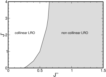
Figure 12: (Color online) Classical phase diagram for the Heisenberg model (1), obtained from numerically solving Eq. (42).

Quantum corrections to the classical phase boundary can be obtained using non-linear spin-wave theory. For $J^{\prime}=1$ this has recently been demonstrated to move the CIT boundary to $J^{\prime\prime}=0.77$ at order $1/S$ (Ref. wang11, ).

Appendix B Effective triplet Hamiltonian in real space

Here we quote the full expressions for the real-space Hamiltonian (6), which can be obtained using straightforward algebra via Eq. (3).

$$\mathcal{H}_{0} = -\frac{3J^{\prime}}{4}\sum_{j}s^{\dagger}_{j}s_{j},$$ (45)

$$\mathcal{H}_{2} = \frac{J^{\prime}}{4}\sum_{j}t^{\dagger}_{j\,\alpha}t_{j\,\alpha}$$ (46)

$$+\frac{1}{4}\sum_{j,n}g_{2}(n)\left[(s_{j}s^{\dagger}_{j+n}t^{\dagger}_{j\,\alpha}t_{j+n\,\alpha}+{\rm H.c.})\right.$$

$$+\left.(s^{\dagger}_{j}s^{\dagger}_{j+n}t_{j\,\alpha}t_{j+n\,\alpha}+{\rm H.c.})\right],$$

$$\mathcal{H}_{3} = \frac{i}{4}\epsilon_{\alpha\beta\lambda}\sum_{j,n}\left\{\left[(s^{\dagger}_{j}t_{j\,\alpha}+t^{\dagger}_{j\,\alpha}s_{j})t^{\dagger}_{j+n\,\beta}t_{j+n\,\lambda}\right.\right.$$ (47)

$$\left.\left.+\,{\rm H.c.}\right]-\;(j\leftrightarrow j+n)\right\},$$

$$\mathcal{H}_{4} = -\frac{1}{4}\epsilon_{\alpha\beta\lambda}\epsilon_{\alpha\mu\nu}\sum_{j,n}g_{4}(n)t^{\dagger}_{j\,\beta}t^{\dagger}_{j+n\,\mu}t_{j+n\,\nu}t_{j\,\lambda},$$ (48)

where the $\sum_{j}$ runs over the sites of the dimerized lattice, and the $g_{m}(n)$ coefficients read

$$g_{2}(n) = (2J^{\prime\prime}-1)\delta_{n,1}-\delta_{n,2}-\delta_{n,3},$$

$$g_{4}(n) = (2J^{\prime\prime}+1)\delta_{n,1}+\delta_{n,2}+\delta_{n,3}.$$

Appendix C Self-consistent equations

Here we derive the self-consistent Eqs. (19)–(20) involved in the harmonic approximation, and Eqs. (28)–(29) related to the HF one. As mentioned in Sec. III, the starting point is the saddle point conditions: (i) $\partial\bar{E}_{0}/\partial N_{0}=0$ and (ii) $\partial\bar{E}_{0}/\partial\mu=0$.

Let us consider the harmonic case. From the expression (16) for the ground state energy, we have

$$\frac{\partial\bar{E}_{0}}{\partial N_{0}}=-\frac{3}{8}J^{\prime}N-\frac{1}{2}\mu N+\frac{3}{2}\sum_{\bf q}\left(\frac{\partial\omega_{\bf q}}{\partial N_{0}}-\frac{\partial A_{\bf q}}{\partial N_{0}}\right).$$ (49)

Since $\partial A_{\bf q}/\partial N_{0}=\partial B_{\bf q}/\partial N_{0}=B_{\bf q}/N_{0}$, see Eqs. (10)–(11), condition (i) yields Eq. (19). Moreover,

$$\frac{\partial\bar{E}_{0}}{\partial\mu}=-\frac{1}{2}N(N_{0}-1)+\frac{3}{2}\sum_{\bf q}\left(\frac{\partial\omega_{\bf q}}{\partial\mu}-\frac{\partial A_{\bf q}}{\partial\mu}\right).$$ (50)

One can easily see that $\partial A_{\bf q}/\partial\mu=-1$ and $\partial\omega_{\bf q}/\partial\mu=-A_{\bf q}/\omega_{\bf q}$, and therefore condition (ii) leads to Eq. (20).

Turning to the Hartree-Fock approximation, the equivalent of Eq. (49) is here given by

$$\frac{\partial\bar{E}^{\rm HF}_{0}}{\partial N_{0}}=-\frac{3}{8}J^{\prime}N-\frac{1}{2}\mu N+\frac{3}{2}\sum_{\bf q}\left(\frac{\partial\bar{\omega}_{\bf q}}{\partial N_{0}}-\frac{\partial\bar{A}_{\bf q}}{\partial N_{0}}\right).$$ (51)

The contribution due to $E^{\rm HF}_{0}$, Eq. (LABEL:hf-coef), can be neglected since it is $\mathcal{O}(\bar{v}^{2}_{\bf q})$ and therefore small compared to the other terms (see discussion in Sec. IV.1). The last term of the above equation can be written as

$$I=\frac{3}{2}\sum_{\bf q}\left(-1+\frac{\bar{A}_{\bf q}}{\bar{\omega}_{\bf q}}\right)\frac{\partial\bar{A}_{\bf q}}{\partial N_{0}}-\frac{\bar{B}_{\bf q}}{\bar{\omega}_{\bf q}}\frac{\partial\bar{B}_{\bf q}}{\partial N_{0}}$$

with

$$\frac{\partial\bar{A}_{\bf q}}{\partial N_{0}} = \frac{B_{\bf q}}{N_{0}}-\frac{1}{N^{\prime}}\sum_{\bf k}\,\gamma_{{\bf k}-{\bf q}}\frac{\partial}{\partial N_{0}}\left(\frac{\bar{A}_{\bf k}}{\bar{\omega}_{\bf k}}\right),$$

$$\frac{\partial\bar{B}_{\bf q}}{\partial N_{0}} = \frac{B_{\bf q}}{N_{0}}-\frac{1}{N^{\prime}}\sum_{\bf k}\,\gamma_{{\bf k}-{\bf q}}\frac{\partial}{\partial N_{0}}\left(\frac{\bar{B}_{\bf k}}{\bar{\omega}_{\bf k}}\right).$$

Assuming that

$$\partial\bar{A}_{\bf q}/\partial N_{0}=\partial\bar{B}_{\bf q}/\partial N_{0}\approx B_{\bf q}/N_{0},$$ (52)

and using the expressions (27), we show that $I\approx(3/N_{0})\sum_{\bf q}B_{\bf q}\bar{v}_{\bf q}\left(\bar{v}_{\bf q}-\bar{u}_{\bf q}\right),$ and therefore Eq. (28) follows from condition (i). Some words about the assumption (52) are here in order: we realize that it is a good approximation as long as $v_{\bf q}$ is small. Indeed, using the relations (27), it is possible to show that

$$\frac{\partial}{\partial N_{0}}\left(\frac{\bar{A}_{\bf k}}{\bar{\omega}_{\bf k}}\right)=\frac{4\bar{u}^{2}_{\bf k}\bar{v}^{2}_{\bf k}}{\bar{\omega}_{\bf k}}\frac{\partial\bar{A}_{\bf q}}{\partial N_{0}}+\frac{2\bar{u}_{\bf k}\bar{v}_{\bf k}}{\bar{\omega}_{\bf k}}\left(\bar{v}^{2}_{\bf q}+\bar{u}^{2}_{\bf q}\right)\frac{\partial\bar{B}_{\bf k}}{\partial N_{0}}.$$

Substituting (52) in the above expression, one can easily see that $\partial\bar{A}_{\bf q}/\partial N_{0}\approx B_{\bf q}/N_{0}+\mathcal{O}(\bar{v}_{\bf k})$. Similar expression holds for $\partial\bar{B}_{\bf q}/\partial N_{0}$.

The analog of Eq. (50) reads

$$\frac{\partial\bar{E}^{\rm HF}_{0}}{\partial\mu}=-\frac{1}{2}N(N_{0}-1)+\frac{3}{2}\sum_{\bf q}\left(\frac{\partial\bar{\omega}_{\bf q}}{\partial\mu}-\frac{\partial\bar{A}_{\bf q}}{\partial\mu}\right).$$ (53)

Here

$$\frac{\partial\bar{A}_{\bf q}}{\partial\mu} = -1-\frac{1}{N^{\prime}}\sum_{\bf k}\,\gamma_{{\bf k}-{\bf q}}\frac{\partial}{\partial\mu}\left(\frac{\bar{A}_{\bf k}}{\bar{\omega}_{\bf k}}\right),$$

$$\frac{\partial\bar{B}_{\bf q}}{\partial\mu} = -\frac{1}{N^{\prime}}\sum_{\bf k}\,\gamma_{{\bf k}-{\bf q}}\frac{\partial}{\partial\mu}\left(\frac{\bar{B}_{\bf k}}{\bar{\omega}_{\bf k}}\right).$$

In order to be consistent with the above approximation, we assume that $\partial\bar{A}_{\bf q}/\partial\mu\approx-1$ and $\partial\bar{B}_{\bf q}/\partial\mu\approx 0$ which implies $\partial\bar{\omega}_{\bf q}/\partial\mu\approx-\bar{A}_{\bf q}/\bar{\omega}_{\bf q}$. Notice that this is indeed a reasonable approximation because condition (ii) yields to nothing else but the conservation (on average) of the total number of bosons per site of the dimerized lattice, i.e., Eq. (29).

References

• (1) S. Sachdev, in: Quantum magnetism, Lecture Notes in Physics Vol. 645, edited by U. Schollwöck, J. Richter, D. J. J. Farnell, and R. A. Bishop (Springer, Berlin 2004); S. Sachdev, Nature Physics 4, 173 (2008).
• (2) G. Misguich and C. Lhuillier, in Frustrated Spin Systems, edited by H. T. Diep (World Scientific, Singapore, 2004); C. Lhuillier, preprint arXiv:cond-mat/0502464.
• (3) L. Balents, Nature 464, 199 (2010).
• (4) P. W. Anderson, Mater. Res. Bull. 8, 153 (1973).
• (5) See, e.g., L. Capriotti, A. E. Trumper, and S. Sorella, Phys. Rev. Lett. 82, 3899 (1999); W. Zheng, J. O. Fjarestad, R. R. P. Singh, R. H. McKenzie, and R. Coldea, Phys. Rev. B 74, 224420 (2006); S. R. White and A. L. Chernyshev, Phys. Rev. Lett. 99, 127004 (2007).
• (6) H.-Y.Yang, A. Läuchli, F. Mila, and K. P. Schmidt, Phys. Rev. Lett. 105, 267204 (2010).
• (7) A. E. Trumper, Phys. Rev. B 60, 2987 (1999).
• (8) J. Merino, R. H. McKenzie, J. B. Marston, and C. H. Chung, J. Phys.: Condens. Matter 11, 2965 (1999).
• (9) Z. Weihong, R. H. McKenzie, and R. R. P. Singh, Phys. Rev. B 59, 14367 (1999).
• (10) R. F. Bishop, P. H. Y. Li, D. J. J. Farnell, and C. E. Campbell, Phys. Rev. B 79, 174405 (2009).
• (11) O. A. Starykh and L. Balents, Phys. Rev. Lett. 98, 077205 (2007).
• (12) S. Ghamari, C. Kallin, S.-S. Lee, and E. S. Sorensen, Phys. Rev. B 84, 174415 (2011).
• (13) A. Weichselbaum and S. R. White, Phys. Rev. B 84, 245130 (2011).
• (14) S. Yunoki and S. Sorella, Phys. Rev. B 74, 014408 (2006); D. Heidarian, S. Sorella, and F. Becca, Phys. Rev. B 80, 012404 (2009).
• (15) J. Reuther and R. Thomale, Phys. Rev. B 83, 024402 (2011).
• (16) C. Xu and S. Sachdev, Phys. Rev. B 79, 064405 (2009).
• (17) P. Hauke, T. Roscilde, V. Murg, J I. Cirac, and R. Schmied, New J. Phys. 13, 075017 (2011).
• (18) R. Coldea, D. A. Tennant, A. M. Tsvelik, and Z. Tylczynski, Phys. Rev. Lett. 86, 1335 (2001).
• (19) T. Ono, H. Tanaka, H. Aruga Katori, F. Ishikawa, H. Mitamura, and T. Goto, Phys. Rev. B 67, 104431 (2003).
• (20) Y. Shimizu, K. Miyagawa, K. Kanoda, M. Maesato, and G. Saito, Phys. Rev. Lett. 91, 107001 (2003); Phys. Rev. B 73, 140407(R) (2006).
• (21) M. Tamura, A. Nakao, and R. Kato, J. Phys. Soc. Jpn. 75, 093701 (2006).
• (22) Y. Shimizu, H. Akimoto, H. Tsujii, A. Tajima, and R. Kato, Phys. Rev. Lett. 99, 256403 (2007).
• (23) T. Itou, A. Oyamada, S. Maegawa, K. Kubo, H. M. Yamamoto, and R. Kato, Phys. Rev. B 79, 174517 (2009).
• (24) M. Tamura and R. Kato, Sci. Technol. Adv. Mater. 10, 024304 (2009).
• (25) T. Itou, A. Oyamada, S. Maegawa, M. Tamura, and R. Kato, Phys. Rev. B 77, 104413 (2008).
• (26) The dimerization pattern in Fig. 1 appears different from the one proposed for EtMe3P[Pd(dmit)2]2 in Ref. dmit01, , but we note that the undistorted phase of EtMe3P[Pd(dmit)2]2 is very close to the isotropic point with the three exchange couplings being equal within 6%, such that the dimer states are nearly degenerate. One of our motivations to choose the dimer pattern of Fig. 1 was to make contact with the staggered dimerized square-lattice model of Refs. wenzel08, ; stag-dimer, .
• (27) S. Sachdev and R. Bhatt, Phys. Rev. B 41, 9323 (1990).
• (28) A. Dutta, B. K. Chakrabarti, and J. K. Bhattacharjee, Phys. Rev. B55, 5619 (1997).
• (29) R. Ramazashvili, Phys. Rev. B60, 7314 (1999).
• (30) A. Kolezhuk and S. Sachdev, Phys. Rev. Lett. 96, 087203 (2006).
• (31) M. E. Zhitomirsky, Phys. Rev. B 73, 100404 (2006).
• (32) T. Giamarchi, C. Rüegg, and O. Tchernyshyov, Nature Phys. 4, 198 (2008).
• (33) S. Wenzel, L. Bogacz, and W. Janke, Phys. Rev. Lett. 101, 127202 (2008).
• (34) L. Fritz, R. L. Doretto, S. Wessel, S. Wenzel, S. Burdin, and M. Vojta, Phys. Rev. B 83, 174416 (2011)
• (35) A. L. Chernyshev and M. E. Zhitomirsky, Phys. Rev. B 79, 144416 (2009).
• (36) A. V. Chubukov and D. K. Morr, Phys. Rev. B 52, 3521 (1995).
• (37) V. N. Kotov, O. Sushkov, W. H. Zheng, and J. Oitmaa, Phys. Rev. Lett. 80, 5790 (1998).
• (38) V. N. Kotov, J. Oitmaa, O. P. Sushkov, and W. H. Zheng, Phys. Rev. B 60, 14613 (1999).
• (39) P. V. Shevchenko, V. N. Kotov, and O. P. Sushkov, Phys. Rev. B 60, 3305 (1999).
• (40) Strictly, the cubic interaction generates both normal and anomalous self-energies which then yield a $2\times 2$ matrix structure of the Dyson equation. However, in the $b$ basis, the anomalous self-energy is small provided that $\bar{v}_{\bf k}$ is small: For selected parameters, we have checked that including the anomalous self-energy in the on-shell approximation changes the triplon energy by less than 1%.
• (41) L. Wang and S. G. Chung, preprint arXiv:1110.0377.