Vector solitons in nonlinear isotropic chiral metamaterials

Abstract

Starting from the Maxwell equations, we used the reductive perturbation method to derive a system of two coupled nonlinear Schrödinger (NLS) equations for the two Beltrami components of the electromagnetic field propagating along a fixed direction in an isotropic nonlinear chiral metamaterial. With single-resonance Lorentz models for the permittivity and permeability and a Condon model for the chirality parameter, in certain spectral regimes, one of the two Beltrami components exhibits a negative-real refractive index when nonlinearity is ignored and the chirality parameter is sufficiently large. We found that, inside such a spectral regime, there may exist a subregime wherein the system of the NLS equations can be approximated by the Manakov system. Bright-bright, dark-dark and dark-bright vector solitons can be formed in that spectral subregime.

1 Introduction

Metamaterials exhibiting a refractive index with a negative real part in certain spectral regimes have been a topic of intense research activity over the last decade [1, 2, 3]. A sufficient condition for the exhibition of a negative-real refractive index (NRRI) by an isotropic dielectric-magnetic material is that both its permittivity $\tilde{\epsilon}(\omega)$ and permeability $\tilde{\mu}(\omega)$ have negative real parts for the same value of the angular frequency $\omega$ [4]. That demanding condition can be relaxed if the isotropic material possesses chirality. In this case, one of the two refractive indices exhibited by such an isotropic chiral material can have a negative real part [5, 6]; besides, the possibility of realizing NRRI materials through the routes of gyrotropy and nonreciprocity [7, Sec. 2.3.4] was considered in the more general context of Faraday chiral materials [5]. Although the electromagnetic (EM) properties of isotropic chiral materials had been studied in detail in the recent past [8, 9, 10], the possibility of isotropic chiral NRRI materials gave fresh impetus [11]. Significant theoretical progress has been reported [12, 13, 14, 15, 16] in comparison to experimental progress [17].

All of the foregoing NRRI materials have been considered to have linear response properties. Nonlinear NRRI materials—of the isotropic achiral type—were introduced [18, 19] shortly after their linear counterparts. Theoretical research has been extensively performed on these nonlinear NRRI materials, as they feature nonlinearity-induced localization of EM waves and soliton formation [20, 21, 22, 23, 24, 25, 26, 27]. Similar effects had been predicted earlier for nonlinear isotropic chiral materials with positive-real refractive indices [28, 29, 30, 31]. The possible incorporation of nonlinearity in isotropic chiral NRRI materials motivated us to investigate soliton formation in these materials.

In this paper, we report on the propagation of an EM field along a fixed direction in an isotropic chiral NRRI material with nonlinear permittivity and permeability of the Kerr type [32]. Furthermore, our analytical approximations may also be useful for analyzing field propagation along the distinguished axis of a nonlinear uniaxial bianisotropic material. We start from the Maxwell equations in the time domain and use the reductive perturbation method (RPM) [33, 34] to derive a system of two coupled nonlinear Schrödinger (NLS) equations for the left-handed and right-handed Beltrami components of the EM field [9]. Then, we adopt (i) the Lorentz model for the linear parts of the relative permittivity and permeability and (ii) the Condon model for the (linear) chirality parameter; see, e.g., Ref. [35] and references therein.

Now, if the chirality parameter is sufficiently large in a certain spectral regime and both dissipation and nonlinearity are ignored, the refractive index for the left/right-handed Beltrami component is real and negative but that for right/left-handed Beltrami component is real and positive [13]. Inside that spectral regime, perturbative nonlinearity of the chosen kind induces a spectral subregime wherein the system of the NLS equations can be approximated by the Manakov system [36]. Since the latter is known to be completely integrable [37, 38, 39], we can predict various classes of exact vector soliton solutions that can be supported in the nonlinear isotropic chiral NRRI material: depending on the type of nonlinearity, namely self-focusing or self-defocusing, we find that bright-bright solitons (for the focusing case), as well as dark-dark and dark-bright solitons (for the defocusing case) can be formed. In all cases, these vector solitons are composed of a Beltrami component with negative-real refractive index and another with a positive-real refractive index.

The paper is organized as follows. In Sec. 2 we present the constitutive relations and use the RPM to derive, from the time-domain Maxwell equations, the system of two coupled NLS equations. In Sec. 3 we show that the coupled NLS equations can be approximated by the Manakov system, and we present various types of vector soliton solutions. We conclude in Sec. 4.

2 Coupled nonlinear Schrödinger equations

2.1 Constitutive relations

In the time domain, the Tellegen constitutive relations of an isotropic chiral material are expressed as [8, 9, 10]

$$\mathbf{D}({\bf r},t)=\int_{-\infty}^{t}\left[\epsilon(\tau)\ast\mathbf{E}({\bf r},t-\tau)+\xi(\tau)\ast\mathbf{H}({\bf r},t-\tau)\right]d\tau\,,$$ (1)

$$\mathbf{B}({\bf r},t)=\int_{-\infty}^{t}\left[\mu(\tau)\ast\mathbf{H}({\bf r},t-\tau)-\xi(\tau)\ast\mathbf{E}({\bf r},t-\tau)\right]d\tau\,,$$ (2)

where $\mathbf{D}({\bf r},t)$ and $\mathbf{B}({\bf r},t)$ are the electric flux density and the magnetic induction field, respectively; $\epsilon(t)$ is the inverse Fourier transform of $\tilde{\epsilon}(\omega)$, and $\mu(t)$ of $\tilde{\mu}(\omega)$; and $\xi(t)$, the inverse Fourier transform of $\tilde{\xi}(\omega)$, accounts for the chirality of the chosen material. Hereafter, ${\bf r}=x\hat{\bf{x}}+y\hat{\bf{y}}+z\hat{\bf{z}}$ is the position vector and $t$ denotes time.

We specify the permittivity and the permeability in the frequency domain in terms of linear and nonlinear components as follows:

$$\tilde{\epsilon}(\omega) = \tilde{\epsilon}_{\ell}(\omega)+\tilde{\epsilon}_{n\ell}(|\mathbf{E}|^{2},|\mathbf{H}|^{2}),\quad\quad$$ (3)

$$\tilde{\mu}(\omega) = \tilde{\mu}_{\ell}(\omega)+\tilde{\mu}_{n\ell}(|\mathbf{E}|^{2},|\mathbf{H}|^{2}),\qquad$$ (4)

The linear components of $\tilde{\epsilon}_{\ell}$ and $\tilde{\mu}_{\ell}$ depend on $\omega$ and can be decomposed into real and and imaginary parts, i.e.,

$$\tilde{\epsilon}_{\ell}(\omega) = \tilde{\epsilon}_{R}(\omega)+i\tilde{\epsilon}_{I}(\omega),$$ (5)

$$\tilde{\mu}_{\ell}(\omega) = \tilde{\mu}_{R}(\omega)+i\tilde{\mu}_{I}(\omega),$$ (6)

where the imaginary parts $\tilde{\epsilon}_{I}$ and $\tilde{\mu}_{I}(\omega)$ account for dissipation. The nonlinear parts $\tilde{\epsilon}_{n\ell}$ and $\tilde{\mu}_{n\ell}$ are assumed to be independent of frequency and depend quadratically but weakly on the magnitudes of both the electric field and the magnetic field. In particular, we consider an isotropic Kerr nonlinearity with

$$\tilde{\epsilon}_{n\ell} = \alpha_{1}|\mathbf{E}|^{2}+\beta_{1}|\mathbf{H}|^{2},$$ (7)

$$\tilde{\mu}_{n\ell} = \alpha_{2}|\mathbf{E}|^{2}+\beta_{2}|\mathbf{H}|^{2},$$ (8)

where $\alpha_{1,2}$ and $\beta_{1,2}$ are scalar Kerr coefficients governing the magnitude of the nonlinearity. These four coefficients are the necessary ones to describe nonlinear wave propagation, in the framework of the NLS model, in an isotropic chiral material; see Sec. 2.3 later in this paper along with Ref. [29] for earlier work. The assumed form of the nonlinear dependence of $\tilde{\epsilon}_{n\ell}$ and $\tilde{\mu}_{n\ell}$ may stem from a Taylor expansion of a more general type of nonlinearity (e.g., a saturable one) [43].

The frequency-domain chirality parameter $\tilde{\xi}(\omega)$ is purely linear, and is defined as

$$\tilde{\xi}(\omega)=\frac{i}{c}\tilde{\kappa}(\omega)=\frac{i}{c}\left[\tilde{\kappa}_{R}(\omega)+i\tilde{\kappa}_{I}(\omega)\right]\,,$$ (9)

where $c$ is the speed of light in free space (vacuum), and the frequency-dependent function $\tilde{\kappa}$ defines the chiral properties of the material, with its imaginary part $\tilde{\kappa}_{I}$ accounting for dissipation together with $\tilde{\epsilon}_{I}$ and $\tilde{\mu}_{I}$.

Finally, we define the complex wave numbers

$$\tilde{k}^{\pm}(\omega) = \frac{\omega}{c}\left(\sqrt{\frac{\tilde{\epsilon}(\omega)\tilde{\mu}(\omega)}{\epsilon_{0}\mu_{0}}}\pm\tilde{\kappa}(\omega)\right)=\tilde{k}_{R}^{\pm}(\omega)+i\tilde{k}_{I}^{\pm}(\omega),$$ (10)

and the complex refractive indices

$$\tilde{n}^{\pm}(\omega)=\frac{c}{\omega}\tilde{k}^{\pm}(\omega)=\tilde{n}_{R}^{\pm}(\omega)+i\tilde{n}_{I}^{\pm}(\omega)\,,$$ (11)

where the superscript $+$ identifies the left-handed Beltrami component and the superscript $-$ identified the right-handed Beltrami component, whereas $\epsilon_{0}$ and $\mu_{0}$ are the permittivity and permeability of free space. With an $\exp(-i\omega t)$ time dependence, if $\tilde{\bf E}({\bf r},\omega)$ and $\tilde{\bf H}({\bf r},\omega)$ are the electric and magnetic field phasors, then the two Beltrami components given by

$$\tilde{\bf Q}^{\pm}({\bf r},\omega)=\frac{1}{2}\left[\tilde{\bf E}({\bf r},\omega){\pm}i\tilde{\eta}_{\ell}(\omega)\tilde{\bf H}({\bf r},\omega)\right],$$ (12)

obey the equations

$$\nabla\times\tilde{\bf Q}^{\pm}({\bf r},\omega)={\pm}\tilde{k}^{\pm}(\omega)\,\tilde{\bf Q}^{\pm}({\bf r},\omega),$$ (13)

where $\tilde{\eta}_{\ell}^{2}(\omega)=\tilde{\mu}_{\ell}(\omega)/\tilde{\epsilon}_{\ell}(\omega)$, and the nonlinear properties have been ignored [9, 10].

2.2 Propagation along the $+z$ axis

Faraday and Ampére–Maxwell equations are, respectively, stated as $\nabla\times{\bf E}({\bf r},t)=-(\partial/\partial t){\bf B}({\bf r},t)$ and $\nabla\times{\bf H}({\bf r},t)=(\partial/\partial t){\bf D}({\bf r},t)$. Let us assume that the EM field is propagating along the $+z$ axis. It then has to be transversely polarized: $\mathbf{E}(z,t)=\hat{\mathbf{x}}E_{x}(z,t)+\hat{\mathbf{y}}E_{y}(z,t)$ and $\mathbf{H}(z,t)=\hat{\mathbf{x}}H_{x}(z,t)+\hat{\mathbf{y}}H_{y}(z,t)$. Furthermore, the field has a carrier angular frequency $\omega_{c}$.

Following the Bohren decomposition of the EM field phasors into left- and right-handed Beltrami components [9, 29] provided in Sec. 2.1, we represent

$$\mathbf{E}(z,t) =\left[\hat{\mathbf{e}}_{+}q^{+}(z,t){\rm e}^{ik^{+}_{c}z}+\hat{\mathbf{e}}_{-}q^{-}(z,t){\rm e}^{ik^{-}_{c}z}\right]{\rm e}^{-i\omega_{c}t}+{\rm c.c.},$$ (14)

$$\mathbf{H}(z,t) =\left[\hat{\mathbf{e}}_{+}p^{+}(z,t){\rm e}^{ik^{+}_{c}z}+\hat{\mathbf{e}}_{-}p^{-}(z,t){\rm e}^{ik^{-}_{c}z}\right]{\rm e}^{-i\omega_{c}t}+{\rm c.c.},$$ (15)

where “c.c.” denotes the complex conjugate, $k^{\pm}_{c}=\tilde{k}^{\pm}(\omega_{c})$, $\hat{\mathbf{e}}_{\pm}=(\hat{\mathbf{x}}\pm i\hat{\mathbf{y}})/\sqrt{2}$, whereas the field envelopes $q^{\pm}(z,t)$ and $p^{\pm}(z,t)$ have to be determined. We also define $k_{c}^{\pm(1)}={d\tilde{k}^{\pm}(\omega)}/{d\omega}|_{\omega=\omega_{c}}$ and $k_{c}^{\pm(2)}={d^{2}\tilde{k}^{\pm}(\omega)}/{d\omega^{2}}|_{\omega=\omega_{c}}$.

2.3 Nonlinear evolution equations

Nonlinear evolution equations for the unknown field envelopes can be found by the reductive perturbation method [33, 34] as follows. We introduce the slow variables

$$Z=\varepsilon^{2}z,\quad\quad T^{\pm}=\varepsilon\left(t-k_{c}^{\pm(1)}z\right),$$ (16)

where $\varepsilon$ is a formal small parameter, defined as the relevant temporal spectral width of the nonlinear term with respect to the spectral width of the quasi-plane-wave dispersion relation [40, 41, 42]. Furthermore, we express $q^{\pm}(z,t)$ and $p^{\pm}(z,t)$ as asymptotic expansions in terms of the parameter $\varepsilon$ as follows:

$$q^{\pm}(Z,T^{\pm}) =q^{\pm}_{0}(Z,T^{\pm})+\varepsilon q^{\pm}_{1}(Z,T^{\pm})+\varepsilon^{2}q^{\pm}_{2}(Z,T^{\pm})+\ldots\,,$$ (17)

$$p^{\pm}(Z,T^{\pm}) =p^{\pm}_{0}(Z,T^{\pm})+\varepsilon p^{\pm}_{1}(Z,T^{\pm})+\varepsilon^{2}p^{\pm}_{2}(Z,T^{\pm})+\ldots\,.$$ (18)

Next, we substitute Eqs. (17) and (18) as well as the constitutive relations into the Faraday and the Ampére–Maxwell equations, and expand $\tilde{\epsilon}_{\ell}(\omega)$, $\tilde{\mu}_{\ell}(\omega)$, and $\tilde{\kappa}_{\ell}(\omega)$ about the angular frequency $\omega_{c}$. Assuming that all members of the set $\left\{\alpha_{1,2},\beta_{1,2},\tilde{\epsilon}_{I},\tilde{\mu}_{I},\tilde{\kappa}_{I}\right\}$ are of order $\mathcal{O}(\varepsilon^{2})$, we obtain the following equations at various orders of $\varepsilon$:

$$\mathcal{O}(\varepsilon^{0}):\,\,\mathbf{W^{\pm}}\mathbf{f}^{\pm}_{0} = \mathbf{0},$$ (19)

$$\mathcal{O}(\varepsilon^{1}):\,\,\mathbf{W^{\pm}}\mathbf{f}^{\pm}_{1} = -i(\mathbf{W^{\pm}})^{\prime}\partial_{T}^{\pm}\mathbf{f}^{\pm}_{0},$$ (20)

$$\mathcal{O}(\varepsilon^{2}):\,\,\mathbf{W^{\pm}}\mathbf{f}^{\pm}_{2} = -i(\mathbf{W^{\pm}})^{\prime}\partial_{T^{\pm}}\mathbf{f}^{\pm}_{1}+\frac{1}{2}(\mathbf{W^{\pm}})^{\prime\prime}\partial^{2}_{T^{\pm}}\mathbf{f}^{\pm}_{0}$$ (21)

$${\pm} \frac{1}{2}k^{\pm(2)}_{c}\mathbf{J}\partial^{2}_{T^{\pm}}\mathbf{f}^{\pm}_{0}\,{\mp}\,i\mathbf{J}\partial_{Z}\mathbf{f}^{\pm}_{0}-\mathbf{A}^{\pm}_{0}-\mathbf{B}\mathbf{f}^{\pm}_{0}.$$

Here and hereafter, the prime denotes the derivative with respect to $\omega$,

$$\mathbf{f}^{\pm}_{j}=\left[\begin{array}[]{c}q^{\pm}_{j}\\[5.0pt] p^{\pm}_{j}\end{array}\right]\,,\quad j\in\left\{0,1,2\right\}\,,$$ (24)

$$\mathbf{W^{\pm}}=\left[\begin{array}[]{cc}\mp k^{\pm}_{c}+\frac{\omega_{c}}{c}\tilde{\kappa}_{R}&\frac{i\omega_{c}}{c}\tilde{\mu}_{R}\\[5.0pt] \frac{i\omega_{c}}{c}\tilde{\epsilon}_{R}&\pm k^{\pm}_{c}-\frac{\omega_{c}}{c}\tilde{\kappa}_{R}\\ \end{array}\right],$$ (27)

$$\mathbf{A}^{\pm}_{0}=i\omega_{c}\left[\begin{array}[]{c}\mu_{0}[\alpha_{2}(|q^{+}_{0}|^{2}+|q^{-}_{0}|^{2})+\beta_{2}(|p^{+}_{0}|^{2}+|p^{-}_{0}|^{2})]p^{\pm}_{0}\\[5.0pt] \epsilon_{0}[\alpha_{1}(|q^{+}_{0}|^{2}+|q^{-}_{0}|^{2})+\beta_{1}(|p^{+}_{0}|^{2}+|p^{-}_{0}|^{2})]q^{\pm}_{0}\\ \end{array}\right],$$ (30)

$$\mathbf{B}=-\frac{\omega_{c}}{c}\left[\begin{array}[]{cc}-i\tilde{\kappa}_{I}&\tilde{\mu}_{I}\\ \tilde{\epsilon}_{I}&i\tilde{\kappa}_{I}\\ \end{array}\right],\quad\mathbf{J}=\left[\begin{array}[]{cc}1&0\\ 0&-1\\ \end{array}\right].$$ (35)

To proceed further, we note that the compatibility conditions required for Eqs. (19)-(21) to be solvable, known also as Fredholm alternatives [33, 40], are $\mathbf{L}^{\pm}\mathbf{W}^{\pm}\mathbf{f}^{\pm}_{0,1,2}=0$, where $\mathbf{L}^{\pm}=[1,\mp i\tilde{Z}_{\ell}]$ is a left eigenvector of $\mathbf{W}^{\pm}$, such that $\mathbf{L}^{\pm}\mathbf{W}^{\pm}=[0,0]$, with $\tilde{Z}_{\ell}=\sqrt{\tilde{\mu}_{R}/\tilde{\epsilon}_{R}}$ being the linear impedance, when dissipation is small enough to be ignored. Note that this impedance is independent of the chirality parameter $\tilde{\kappa}$ [10].

The zeroth-order Eq. (19) provides the following three results. First, the solution $\mathbf{f}^{\pm}_{0}$ has the form:

$$\mathbf{f}^{\pm}_{0}=\mathbf{R}^{\pm}\phi^{\pm}(Z,T^{\pm}),$$ (36)

where the scalar function $\phi^{\pm}(Z,T^{\pm})$ has to be determined and $\mathbf{R}^{\pm}=[1,\mp i\tilde{Z}_{\ell}^{-1}]^{\rm T}$ is a right eigenvector of $\mathbf{W}^{\pm}$, i.e., $\mathbf{W}^{\pm}\mathbf{R}^{\pm}=[0,0]^{\rm T}$. Second, by using the compatibility condition $\mathbf{L}^{\pm}\mathbf{W}^{\pm}\mathbf{f}^{\pm}_{0}=0$ and Eq. (36), we obtain $\mathbf{L}^{\pm}\mathbf{W}^{\pm}\mathbf{R}^{\pm}=0$, which is actually equivalent to Eq. (10). Third, the respective zeroth-order Beltrami components of the electric and magnetic fields are proportional to each other, namely, $q^{\pm}_{0}=\pm i\tilde{Z}_{\ell}p^{\pm}_{0}$ [10].

Next, at $\mathcal{O}(\varepsilon^{1})$, the compatibility conditions for Eq. (20) result in $\mathbf{L}^{\pm}(\mathbf{W}^{\pm})^{\prime}\mathbf{R}^{\pm}=0$; equivalently,

$$2(ck_{c}^{\pm}\mp\omega_{c}\tilde{\kappa}_{R})(c\tilde{k}^{\pm}\mp\omega\tilde{\kappa}_{R})^{\prime}\big{|}_{\omega=\omega_{c}}=(\omega^{2}\tilde{\epsilon}_{R}\tilde{\mu}_{R})^{\prime}\big{|}_{\omega=\omega_{c}}.$$ (37)

The foregoing equations yield the group speeds $v^{\pm}_{g}\equiv 1/k_{c}^{\pm(1)}$, which can also be derived from Eq. (10). Furthermore, Eqs. (20) and (36) together indicate that $\mathbf{f}^{\pm}_{1}$ has the form:

$$\mathbf{f}^{\pm}_{1}=i(\mathbf{R}^{\pm})^{\prime}\partial_{T^{\pm}}\phi^{\pm}(Z,T^{\pm})+\mathbf{R}^{\pm}\psi^{\pm}(Z,T^{\pm}),$$ (38)

where the scalar function $\psi^{\pm}(Z,T^{\pm})$ can be determined at a higher-order approximation; see, e.g., Ref. [27].

Next, at order $\mathcal{O}(\varepsilon^{2})$, the compatibility conditions for Eq. (21), combined with Eqs. (36) and (38), yield the coupled NLS equations

$$i\partial_{Z}\phi^{\pm}-\frac{1}{2}k_{c}^{\pm(2)}\,\partial^{2}_{T^{\pm}}\phi^{\pm}+\gamma\left(|\phi^{+}|^{2}+|\phi^{-}|^{2}\right)\phi^{\pm}=-i\tilde{\Gamma}^{\pm}\phi^{\pm},$$ (39)

where $k_{c}^{\pm(2)}$ can be obtained from Eq. (37). In this equation, the nonlinearity coefficient

$$\gamma=\frac{\omega_{c}}{2}[\epsilon_{0}(\alpha_{1}\tilde{Z}_{\ell}+\beta_{1}\tilde{Z}_{\ell}^{-1})+\mu_{0}(\alpha_{2}\tilde{Z}_{\ell}+\beta_{2}\tilde{Z}_{\ell}^{-3})]$$ (40)

depends linearly on the scalar Kerr coefficients $\alpha_{1,2}$ and $\beta_{1,2}$, and the loss coefficients $\tilde{\Gamma}^{\pm}$ are given as follows:

$$\tilde{\Gamma}^{\pm}=\omega_{c}\left(\frac{\tilde{\epsilon}_{I}\tilde{\mu}_{R}+\tilde{\epsilon}_{R}\tilde{\mu}_{I}}{2\sqrt{\tilde{\epsilon}_{R}\tilde{\mu}_{R}}}\pm\frac{\tilde{\kappa}_{I}}{c}\right).$$ (41)

2.4 Relation with the Manakov system

Knowledge of $\phi^{\pm}$ obtained from solving Eqs. (39) immediately yields $q^{\pm}_{0}=\phi^{\pm}$ and $p^{\pm}_{0}=\mp i\tilde{Z}_{\ell}^{-1}\phi^{\pm}$, by virtue of Eq. (36), similarly to the case of a linear material.

Let us now analyze Eqs. (39) in more detail. First, measuring length $z$, retarded time $T=t-z/v_{g}^{+}$, and the intensities $|\phi^{\pm}|^{2}$ in units of a characteristic length $L^{+}=t_{0}^{2}/|k^{+(2)}_{c}|$, a characteristic time $t_{0}$, and $L^{+}/|\gamma|$, respectively, we reduce Eqs. (39) to the following dimensionless form:

$$i\partial_{Z}\phi^{+}-\frac{s}{2}\partial_{T}^{2}\phi^{+}+\sigma\left(|\phi^{+}|^{2}+|\phi^{-}|^{2}\right)\phi^{+}=-i\Gamma^{+}\phi^{+},$$ (42)

$$i\left(\partial_{Z}\phi^{-}-\delta\,\partial_{T}\phi^{-}\right)-\frac{d}{2}\partial_{T}^{2}\phi^{-}+\sigma\left(|\phi^{+}|^{2}+|\phi^{-}|^{2}\right)\phi^{-}=-i\Gamma^{-}\phi^{-}.$$ (43)

The parameters involved in the foregoing equations are defined as follows:

$$\delta =t_{0}\frac{k^{+(1)}_{c}-k^{-(1)}_{c}}{|k^{+(2)}_{c}|},\quad d=\frac{k^{-(2)}_{c}}{|k^{+(2)}_{c}|},\quad s=\frac{k^{+(2)}_{c}}{|k^{+(2)}_{c}|},$$

$$\sigma =\gamma/|\gamma|,\quad\Gamma^{\pm}=L^{+}\tilde{\Gamma}^{\pm}.$$ (44)

Since all nonlinearity coefficients in the $\pm$ components of Eq. (39) are equal to $\gamma$, the latter parameter was absorbed by our normalization; this way, the nonlinearity coefficients in the dimensionless Eqs. (42) are (43) are equal to the sign of $\gamma$. Furthermore, as $s={\rm sign}\left[k^{+(2)}_{c}\right]$, the foregoing NLS system is characterized by (i) the parameter $\delta$, which represents the mismatch between the group speeds of the two Beltrami components; (ii) the normalized dispersion parameter $d$ for the field $\phi^{-}$; and (iii) the linear loss parameters $\Gamma^{\pm}$.

In the most general case ($\delta\neq 0$, $d\neq\pm 1$ and $\Gamma^{\pm}\neq 0$), the system of Eqs. (42) and (43) is not integrable. The same is true even if $\Gamma^{+}=\Gamma^{-}=0$; however, for certain values of the linear constitutive parameters and the nonlinearity coefficient $\gamma$, one can find, either analytically or numerically, various types of vector solitons (such as bright-bright, dark-dark, or dark-bright ones), as can be gathered from Refs. [43, 45].

Provided $\delta=0$, $d=s$ and $\Gamma^{\pm}=0$, Eqs. (42) and(43) reduce to the Manakov system [36]. In our case, the latter takes the generic form of a vector NLS equation, which can be expressed as

$$i\partial_{Z}{\bf u}-\frac{s}{2}\partial_{T}^{2}{\bf u}+\sigma|{\bf u}|^{2}{\bf u}=\bf{0},$$ (45)

where ${\bf u}(Z,T)=\left[\phi^{+}(Z,T),\phi^{-}(Z,T)\right]^{T}$. The Manakov system is known to be completely integrable [37, 38, 39]; in fact, it can be integrated by extending the inverse scattering transform method that has been used to integrate the scalar NLS equation [46, 47]. The Manakov system also admits vector $N$-soliton solutions [48, 49, 50, 51, 52, 53].

In the following section, we show that it is possible to find physically relevant conditions allowing us to approximate the general system of the NLS Eqs. (42) and (43) to the Manakov system (45) and investigate conditions for the existence of various types of vector solitons supported by a nonlinear isotropic chiral material.

3 Vector solitons

We considered a certain type of isotropic chiral material that conforms to the single-resonance Lorentz models for the linear parts of permittivity and permeability, and to the Condon model for the chirality parameter (see, e.g., Ref. [35] and references therein) as follows:

$$\tilde{\epsilon}_{\ell}(\omega) = \epsilon_{0}\left(1-\frac{\omega_{p}^{2}}{\omega^{2}-\omega_{\epsilon}^{2}+2i\delta_{\epsilon}\omega}\right),$$ (46)

$$\tilde{\mu}_{\ell}(\omega) = \mu_{0}\left(1-\frac{\omega_{m}^{2}}{\omega^{2}-\omega_{\mu}^{2}+2i\delta_{\mu}\omega}\right),$$ (47)

$$\tilde{\kappa}(\omega) = \frac{acZ_{0}^{-1}\omega}{\omega^{2}-\omega_{\kappa}^{2}+2i\delta_{\kappa}\omega}.$$ (48)

Here, $Z_{0}=\sqrt{\mu_{0}/\epsilon_{0}}$ is the intrinsic impedance of free space; $\{\omega_{\epsilon},\delta_{\epsilon}\}$, $\{\omega_{\mu},\delta_{\mu}\}$, and $\{\omega_{\kappa},\delta_{\kappa}\}$ are the resonance angular frequencies and linewidths of $\tilde{\epsilon}_{\ell}$, $\tilde{\mu}_{\ell}$, and $\tilde{\kappa}$, respectively; while $\omega_{p}$ and $\omega_{m}$ characterize the oscillator strengths of respective transitions in $\tilde{\epsilon}_{\ell}$ and $\tilde{\mu}_{\ell}$. Finally, $a$ is the rotatory strength of the resonance in the Condon model, which measures the degree of chirality. We note that the Lorentz model is a widely used fundamental model, describing the dispersive nature of permittivity and permeability, also accounting for the presence of a single resonance frequency. On the other hand, the Condon model is generally used to represent the dispersive nature of chirality; the Condon model in the form of Eq. (48) is such that the real (imaginary) part of $\tilde{\kappa}(\omega)$ is an odd (even) function of frequency [54, 55], and obeys causality restrictions.

Next, we used Eqs. (46), (47) and (48), as well as the dispersion relations (10), to determine the refractive indices $\tilde{n}^{\pm}$ [cf. Eq. (11)] and the parameters involved in the NLS equations [cf. Eq. (44)]. All numerical results presented were computed for the following values of parameters: $\omega_{p}=0.9\omega_{\epsilon}$, $\omega_{m}=0.8\omega_{\epsilon}$, $\omega_{\mu}=0.8\omega_{\epsilon}$, $\omega_{\kappa}=0.6\omega_{\epsilon}$, $\delta_{\epsilon}=\delta_{\mu}=\delta_{\kappa}=10^{-3}\omega_{\epsilon}$, and $a=0.5\omega_{\epsilon}/c$. Note that all resonance angular frequencies and linewidths are normalized to the resonance angular frequency $\omega_{\epsilon}$ of $\tilde{\epsilon}_{\ell}$, which was taken to be the largest resonance angular frequency in the constitutive description of the chiral material. Other parameter values led to qualitatively similar results.

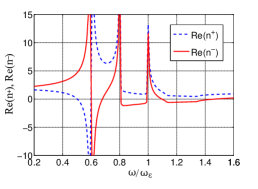
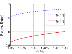
Figure 1: (Color online) Left panel: ${\rm Re}(\tilde{n}^{-})$ (solid red line) and ${\rm Re}(\tilde{n}^{+})$ (dashed blue line) in the spectral regime $(0.2\omega_{\epsilon},1.6\omega_{\epsilon})$. The constitutive parameters used for these data are presented at the beginning of Sec. 3. Three distinct spectral regimes exist wherein ${\rm Re}(\tilde{n}^{-})<0$ and ${\rm Re}(\tilde{n}^{+})>0$. Right panel: Magnification of left panel in the spectral subregime $(1.35\omega_{\epsilon},1.47\omega_{\epsilon})$, wherein not only are ${\rm Re}(\tilde{n}^{-})<0$ and ${\rm Re}(\tilde{n}^{+})>0$, but the NLS Eqs. (42) and (43) can also be approximated by the Manakov system (45).

For the chosen parameters with $a>0$, spectral regimes exist where the refractive indices are $\tilde{n}^{-}<0$ and $\tilde{n}^{+}>0$ if $a\gtrsim a_{c1}=5\times 10^{-3}\omega_{\epsilon}/c$. In the top panel of Fig. 1 we show an example of the frequency dependences of $\tilde{n}^{-}$ and $\tilde{n}^{+}$ for $a=0.5\omega_{\epsilon}/c$. In fact, if the chirality parameter is sufficiently large, i.e., $a\gtrsim a_{c2}=0.1\omega_{\epsilon}/c$, then there exists a certain spectral subregime located to the right of the largest resonance angular frequency $\omega_{\epsilon}$, such that $\tilde{n}^{-}<0$, $\tilde{n}^{+}>0$, and the NLS Eqs. (42) and (43) can be approximated by the Manakov system (45). Hence, this spectral regime is referred to as the Manakov regime in the remainder of this paper. In the particular case of $a=0.5\omega_{\epsilon}/c$, the Manakov regime is $(1.35\omega_{\epsilon},1.47\omega_{\epsilon})$; the dependencies of $\tilde{n}^{-}$ and $\tilde{n}^{+}$ on $\omega$ in this regime are illustrated in the bottom panel of Fig. 1. Here we should note that increase of $a$ above the characteristic value $a_{c2}$ results in the increase of the bandwidth of the Manakov regime; for example, when $a=1$, the Manakov regime is $(1.35\omega_{\epsilon},1.73\omega_{\epsilon})$.

If the sign of $a$ is changed, then a role-reversal occurs in that $\tilde{n}^{+}<0$ and $\tilde{n}^{-}>0$ in the Manakov regime. Although we have maintained $a>0$ in the remainder of this section, the case of $a<0$ can be treated analogously.

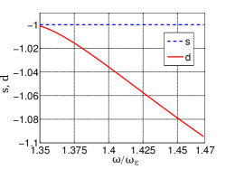
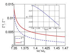
Figure 2: (Color online) Left panel: Normalized dispersion coefficients $s$ (dashed blue line) and $d$ (solid red line) of the NLS Eqs. (42)-(43), defined in Eqs. (44), in the Manakov regime $(1.35\omega_{\epsilon},1.47\omega_{\epsilon})$. Right panel: Normalized loss coefficients, $\Gamma^{+}$ (dashed blue line) and $\Gamma^{-}$ (solid red line) in the Manakov regime. Inset shows the group-speed-mismatch coefficient $\delta$.

In the Manakov regime $d\approx s$, while $\delta\approx 0$ and $\Gamma^{\pm}\approx 0$. This is confirmed by the data presented in Fig. 2. Whereas $d\approx-1$, the maximum deviation between $s$ and $d$ (for $\omega=1.47\omega_{\epsilon}$) is than $10\%$. Furthermore, $\Gamma^{\pm}$ are of order of $10^{-3}$ while $\delta$ is of order of $10^{-2}$. Thus, taking into account that the other coefficients in Eqs. (42) and (43) are equal to $\pm 1$, we can safely conclude that, in a first approximation, our system can be well approximated by the Manakov system (45).

Here it should be noted that, following the foregoing arguments, the (small) effects of the group-speed mismatch between the two Beltrami components and the linear losses can be studied analytically by means of the perturbation theory for solitons; see, e.g., Ref. [56]. However, such a study is beyond the scope of this work. In any case, some estimations concerning, e.g., the role of losses can already be made, based on the linear, dispersionless part of the NLS Eqs. (42)-(43): one expects that the Beltrami fields $\phi^{\pm}$ decay as $\exp(-\Gamma^{\pm}Z)$. To further elaborate on this estimation, however, one would employ real world parameter values, which are not currently available (since experiments on isotropic nonlinear chiral metamaterials considered herein have not been performed so far).

The reduction of Eqs. (42) and (43) to the Manakov system allows us to predict different types of exact vector solitons that can propagate in an isotropic chiral NRRI material. In particular, taking into regard that $s=d=-1$, there are two different cases, depending on the sign $\sigma$ of the nonlinearity coefficient $\gamma$:

• $\sigma=+1$, i.e., the effective Kerr nonlinearity in the Manakov system is self-focusing, and

• $\sigma=-1$, i.e., the effective Kerr nonlinearity is self-defocusing.

3.1 Self-focusing nonlinearity in the Manakov regime

When $s=d=-1$, $\sigma=+1$, and the boundary conditions associated with Eq. (45) are $\phi^{\pm}\rightarrow 0$ as $T\rightarrow 0$, there exist exact bright-bright soliton solutions, i.e., both Beltrami components take the form of bright solitons. Following Refs. [49, 50], we may find such solutions by using the traveling-wave ansatz

$$\phi^{+}(Z,T) = u_{1}(\xi)\exp\left[i(1+C^{2}/2)Z+iCT\right],$$ (49)

$$\phi^{-}(Z,T) = u_{2}(\xi)\exp\left[i(q^{2}+C^{2}/2)Z+iCT\right],$$ (50)

where $\xi=\sqrt{2}(T-CZ)$, the parameter $C$ sets the (common) speed of both components of the traveling wave in the $(Z,T)$-plane, $q$ is an arbitrary parameter connected with the wave number of the right-handed Beltrami component, and $u_{1,2}$ are unknown real functions.

Introducing the ansatz comprising Eqs. (49) and (50) into the Manakov system (45), we obtain the following system of ordinary differential equations (ODEs) for $u_{1}$ and $u_{2}$:

$$\frac{d^{2}u_{1}}{d\xi^{2}}-u_{1}+(u_{1}^{2}+u_{2}^{2})u_{1}=0,$$ (51)

$$\frac{d^{2}u_{2}}{d\xi^{2}}-q^{2}u_{2}+(u_{1}^{2}+u_{2}^{2})u_{2}=0.$$ (52)

The simplest exact solution to this system has either $u_{1}\equiv 0$ or $u_{2}\equiv 0$, i.e., either

$$u_{1} = 0,\quad u_{2}=\sqrt{2}q{\rm sech}(q\xi)$$ (53)

or

$$u_{1} = \sqrt{2}{\rm sech}(\xi),\quad u_{2}=0.$$ (54)

This solution can be generalized to the case wherein both $u_{1}$ and $u_{2}$ are nontrivial [49, 50]. Particularly, if $q=1$, a simple one-parameter family of such solutions is composed of symmetric, single-humped bright solitons of the following form:

$$u_{1}=\sqrt{2}\cos\theta{\rm sech}(\xi),\quad u_{2}=\sqrt{2}\sin\theta{\rm sech}(\xi),$$ (55)

where $\theta$ is an arbitrary parameter. On the other hand, if $0<q<1$, the soliton is

$$u_{1} = \frac{\sqrt{2(1-q^{2})}\cosh(q\xi)}{\cosh(\Delta\xi)\cosh(q\xi)-q\sinh(\Delta\xi)\sinh(q\xi)},$$ (56)

$$u_{2} = \frac{-q\sqrt{2(1-q^{2})}\sinh(\Delta\xi)}{\cosh(\Delta\xi)\cosh(q\xi)-q\sinh(\Delta\xi)\sinh(q\xi)},$$ (57)

where $\Delta\xi\equiv\xi-\xi_{0}$ and $\xi_{0}$ is an arbitrary constant. The solutions (56) and (57) are generally asymmetric; however. $u_{1}$ is symmetric but $u_{2}$ is antisymmetric when $\xi_{0}=0$. Other solution branches, such as soliton bound states and wave- and daughter-wave solutions (for $u_{1}\ll u_{2}$ or $u_{2}\ll u_{1}$), have also been found; see, e.g., Refs. [49, 50], as well as the book [43] and references therein.

3.2 Self-defocusing nonlinearity in the Manakov regime

Let us now change the sign of $\sigma$ to $\sigma=-1$ and keep $s=d=-1$. Now, there exist both dark-dark solitons (where both the Beltrami components take the form of dark solitons) and dark-bright ones (where one Beltrami component is a dark soliton and the other is a bright soliton).

Dark-dark soliton solutions of the Manakov system (45), with boundary conditions $|\phi^{\pm}|\rightarrow\mu_{\pm}$ as $T\rightarrow 0$, where $\mu_{\pm}$ are the amplitudes of the continuous-wave (cw) backgrounds carrying the dark solitons, can be expressed in the following general form [52, 51]:

$$\phi^{\pm}(Z,T)=\mu_{\pm}\{\cos\varphi_{\pm}\tanh[\nu(T-VZ)]+i\sin\varphi_{\pm}\}$$

$$\times\exp\left[i\left(\frac{\eta_{\pm}^{2}}{2}+|\mu_{+}|^{2}+|\mu_{-}|^{2}\right)Z+i\eta_{\pm}T\right],$$ (58)

where $\nu$ and $V$ are the (common) inverse width and speed of dark solitons, while $\eta_{\pm}$ are constants connected to the background angular frequency $\omega_{c}$ and wave numbers $k^{\pm}_{c}$. The phase angles $\varphi_{\pm}=\tan^{-1}[(\eta_{\pm}-V)/\nu]$ are connected with the rest of the soliton parameters according to the relations $\nu^{2}=\mu_{+}^{2}\cos^{2}\varphi_{+}+\mu_{-}^{2}\cos^{2}\varphi_{-}$, while the soliton intensities are as follows:

$$|\phi^{\pm}|^{2}=\mu_{\pm}^{2}-\nu^{2}{\rm sech}^{2}[\nu(T-VZ)].$$ (59)

Finally, for the same case ($\sigma=-1$), we present the exact analytical dark-bright soliton solutions of the Manakov system (45) [48, 52]:

$$\phi^{+}(Z,T) = \phi_{0}\{\cos\varphi\tanh[D(T-C_{s}Z)]+i\cos\varphi\}$$ (60)

$$\times \exp[i\Omega T+i(\Omega^{2}+\phi_{0}^{2})Z],$$

$$\phi^{-}(Z,T) = \eta\,{\rm sech}[D(T-C_{s}Z)]$$ (61)

$$\times \exp\{iC_{s}T+i[(D^{2}-C_{s}^{2})/2-\phi_{0}^{2}]Z\},$$

where $\phi^{+}$ and $\phi^{-}$ correspond, respectively, to the dark and bright soliton components; $\phi_{0}$ is the amplitude of the cw background carrying the dark soliton; $\varphi=\tan^{-1}[(\Omega-C_{s})/D]$ is the dark soliton’s phase angle; $D$ and $C_{s}$ denote the (common) inverse width and speed of both components; $\Omega$ sets the frequency of the dark-soliton component; and $\eta$ is the bright-soliton amplitude, with $\eta^{2}=\phi_{0}^{2}\cos^{2}\varphi-D^{2}$. In the limiting case of $\eta\rightarrow 0$, the bright soliton component vanishes and the inverse width of the dark soliton becomes $D=\phi_{0}\cos\varphi$; this way, Eq. (60) describes the single dark soliton solution of the defocusing NLS equation [44, 45]. It is important to stress here that the dark-bright soliton of Eqs. (60) and (61) is a generic example of a symbiotic soliton: the bright-soliton component exists only due to the coupling with the dark soliton and would not be supported otherwise, due to the fact that the NLS equation for $\phi^{-}$ features a self-defocusing nonlinearity.

Finally, we note in passing that other soliton solutions of the Manakov Eqs. (45) can be systematically constructed by employing the symmetries of the system (such as the SU(2) rotational symmetry) [53].

4 Conclusions

In conclusion, we have studied the propagation of electromagnetic pulses in isotropic chiral NRRI materials with Kerr nonlinearity. We have employed the reductive perturbation theory to derive a system of two coupled nonlinear Schrödinger (NLS) equations for the envelopes of the two Beltrami components of the EM field. Assuming a single-resonance double Lorentz model for the effective permittivity and permeability of the medium, as well as a Condon model for the chirality parameter, we have shown that if the characteristic chirality parameter is sufficiently large, then the material exhibits a negative-real refractive index for the right/left-handed Beltrami component in certain spectral regimes whereas the left/right-handed Beltrami component does not.

Furthermore, we have shown that in a certain subregime inside such a spectral regime, the system of the NLS equations (which is non-integrable in general) may be approximated well by the completely integrable Manakov system. This way, we have predicted various types of vector solitons, such as bright-bright, dark-dark or dark-bright ones, that can be formed in the chosen type of chiral material. Let us emphasize that, in all cases, the presented vector solitons are composed by a Beltrami component that features negative-real refractive index and another Beltrami component that features a positive-real refractive index.

The propagation of the predicted vector soliton solutions needs to be examined by direct numerical simulations in the framework of the Maxwell equations. Furthermore, a relevant future challenge is the analysis of pulse propagation in the bianisotropic [5, 57] counterparts of the isotropic materials we have discussed here. For that purpose, our work can be emulated in three steps as follows. In the first step, one has to obtain explicit plane wave solutions and associated dispersion relations, similar to the ones in Eqs. (10). In the secon step, one has to consider propagation of wavepackets, similar to Eqs. (14) and (15), along a fixed direction (identified by the $z$-axis in our work) of the linearized material — see, e.g., Ref. [57]. The third and final step is to apply the methodology of Section 2.3 to derive a vector NLS-type model (and, in the best-case scenario, a Manakov system) describing nonlinear pulse propagation in the nonlinear material. Also, another interesting possibility would be to apply the derived results in the case of pulse propagation inside a layered chiral [58, 59] or a layered bianisotropic material [60, 61]. For this purpose, one should first find expressions for the EM field components inside each homogeneous layer (relying, e.g., on plane waves for the linear layers, and nonlinear periodic waves or solitons for the nonlinear layers) and then impose the boundary conditions at the interfaces. Finally, our work may be exploited for the analysis of pulse propagation inside composite materials comprising linear chiral and nonlinear dielectric materials [62]. Such studies are currently in process and relevant results will be reported in the future.

References

References

- [1] S. A. Ramakrishna, Rep. Prog. Phys. 68, 449 (2005).
- [2] N. L. Litchinitser and V. M. Shalaev, J. Opt. Soc. Am. B 26, B161 (2009).
- [3] W. Withayachumnankul and D. Abbott, IEEE Photon. J. 1, 99 (2009).
- [4] R. A. Depine and A. Lakhtakia, Microw. Opt. Technol. Lett. 41, 315 (2004).
- [5] T. G. Mackay and A. Lakhtakia, Phys. Rev. E 69, 026602 (2004).
- [6] J. B. Pendry, Science 306, 1353 (2004).
- [7] T.G. Mackay and A. Lakhtakia, Electromagnetic Anisotropy and Bianisotropy (World Scientific, Singapore, 2010).
- [8] A. Lakhtakia, V. K. Varadan, and V. V. Varadan, Time-Harmonic Electromagnetic Fields in Chiral Media (Springer, Berlin, 1989).
- [9] A. Lakhtakia, Beltrami Fields in Chiral Media (World Scientific, Singapore, 1994).
- [10] I. V. Lindell, A. H. Sihvola, S. A. Tretyakov, and A. J. Viitanen, Electromagnetic Waves in Chiral and Bi-isotropic Media (Artech House, Boston, 1994).
- [11] T. G. Mackay and A. Lakhtakia, SPIE Rev. 1, 018003 (2010).
- [12] S. Tretyakov, A. Sihvola, and L. Jylhä, Photon. Nanostruct. 3, 107 (2005).
- [13] T. G. Mackay, Microwave Opt. Technol. Lett. 45, 120 (2005).
- [14] V. Yannopapas, J. Phys. C: Condens. Mater. 18, 6833 (2006).
- [15] T. G. Mackay and A. Lakhtakia, Microwave Opt. Technol. Lett. 49, 1245 (2007).
- [16] W. Dong, and L. Gao, J. Appl. Phys. 104, 023537 (2008).
- [17] B. Wang, J. Zhou, T. Koschny, and C. M. Soukoulis, Appl. Phys. Lett. 94, 151112 (2009).
- [18] A. A. Zharov, I. V. Shadrivov, and Yu. S. Kivshar, Phys. Rev. Lett. 91, 037401 (2003).
- [19] V. M. Agranovich, Y. R. Shen, R. H. Baughman, and A. A. Zakhidov, Phys. Rev. B 69, 165112 (2004).
- [20] N. Lazarides, and G. P. Tsironis, Phys. Rev. E 71, 036614 (2005).
- [21] I. Kourakis, and P. K. Shukla, Phys. Rev. E 72, 016626 (2005).
- [22] M. Marklund, P. K. Shukla, L. Stenflo, and G. Brodin, Phys. Lett. A 341, 231 (2005).
- [23] I. V. Shadrivov and Y. S. Kivshar, J. Opt. A: Pure Appl. Opt. 7, S68 (2005).
- [24] N. L. Tsitsas, T. P. Horikis, Y. Shen, P. G. Kevrekidis, N. Whitaker, and D. J. Frantzeskakis, Phys. Lett. A 374, 1384 (2010).
- [25] M. Scalora, M. S. Syrchin, N. Akozbek, E. Y. Poliakov, G. D’Aguanno, N. Mattiucci, M. J. Bloemer, and A. M. Zheltikov, Phys. Rev. Lett. 95, 013902 (2005).
- [26] S. C. Wen, Y. W. Wang, W. H. Su, Y. J. Xiang, X. Q. Fu, and D. Y. Fan, Phys. Rev. E 73, 036617 (2006).
- [27] N. L. Tsitsas, N. Rompotis, I. Kourakis, P. G. Kevrekidis, and D. J. Frantzeskakis, Phys. Rev. E 79, 037601 (2009).
- [28] F. G. Bass, G. Ya. Slepyan, S. A. Maksimenko, and A. Lakhtakia, Microw. Opt. Technol. Lett. 9, 218 (1995).
- [29] G. Ya. Slepyan, S. A. Maksimenko, F. G. Bass, and A. Lakhtakia, Phys. Rev. E 52, 1049 (1995).
- [30] K. Hayata and M. Koshiba, IEEE Trans. Microw. Theory Tech. 43, 1814 (1995).
- [31] D. J. Frantzeskakis, I. G. Stratis, and A. N. Yannacopoulos, Phys. Scr. 66, 280 (2002).
- [32] P. Weinberger, Philos. Mag. Lett. 88, 897 (2008).
- [33] T. Taniuti, Prog. Theor. Phys. Suppl. 55, 1 (1974).
- [34] H. Leblond, J. Phys. B: At. Mol. Opt. Phys. 41, 043001 (2008).
- [35] S. A. Maksimenko, G. Ya. Slepyan, and A. Lakhtakia, J. Opt. Soc. Am. A 14, 894 (1997).
- [36] S. V. Manakov, Zh. Eksp. Teor. Fiz. 65, 505 (1973) [Sov. Phys. JETP 38, 248 (1974)].
- [37] V. E. Zakharov and S. V. Manakov, Zh. Eksp. Teor. Fiz. 71, 203 (1976) [Sov. Phys. JETP 42, 842 (1976)].
- [38] V. E. Zakharov and E. I. Schulman, Physica D 4, 270 (1982).
- [39] V. G. Makhan kov and O. K. Pashaev, Theor. Math. Phys. 53, 979 (1982).
- [40] Y. Kodama, J. Stat. Phys. 39, 597 (1985).
- [41] Y. Kodama and A. Hasegawa, IEEE J. Quantum Electron. 23, 510 (1987).
- [42] M. J. Potasek, J. Appl. Phys. 65, 941 (1989).
- [43] Yu. S. Kivshar and G. P. Agrawal, Optical Solitons: From Fibers to Photonic Crystals (Academic Press, 2003).
- [44] Yu. S. Kivshar and B. Luther-Davies, Phys. Rep. 298, 81 (1998).
- [45] D. J. Frantzeskakis, J. Phys. A: Math. Theor. 43, 213001 (2010).
- [46] V. E. Zakharov and A. B. Shabat, Zh. Eksp. Teor. Fiz. 61, 118 (1971) [Sov. Phys. JETP 34, 62 (1971)].
- [47] V. E. Zakharov and A. B. Shabat, Zh. Eksp. Teor. Fiz. 64, 1627 (1973) [Sov. Phys. JETP 37, 823 (1973)].
- [48] R. Radhakrishnan and M. Lakshmanan, J. Phys. A: Math. Gen. 28, 2683 (1995).
- [49] M. Haelterman and A. Sheppard, Phys. Rev. E 49, 3376 (1994).
- [50] J. Yang, Physica D 108, 92 (1997).
- [51] Yu. S. Kivshar and S. K. Turitsyn, Opt. Lett. 18, 337 (1993).
- [52] A. P. Sheppard and Yu. S. Kivshar, Phys. Rev. E 55, 4773 (1997).
- [53] Q. H. Park and H. J. Shin, Phys. Rev. E 61, 3093 (2000).
- [54] C. A. Emeis, L. J. Oosterhoof and G. de Vries, Proc. R. Soc. Lond. A 297, 54 (1967).
- [55] F. Guérin and A. Lakhtakia, J. Phys. III France 5, 913 (1995).
- [56] Yu. S. Kivshar and B. A. Malomed, Rev. Mod. Phys. 61, 763 (1989).
- [57] T. G. Mackay and A. Lakhtakia, Prog. Opt. 51, 121 (2008).
- [58] A. Lakhtakia, V. K. Varadan and V. V. Varadan, Int. J. Engg. Sci. 27, 1267 (1989).
- [59] A. Lakhtakia, V. K. Varadan and V. V. Varadan, Z. Naturforsch. A 45, 639 (1990).
- [60] J. L. Tsalamengas, IEEE Trans. Microw. Theory Tech. 40, 1870 (1992).
- [61] A. F. Konstantinova, K. K. Konstantinov, B. V. Nabatov and E. A. Evdishchenko, Crystallogr. Rep. 47, 645 (2002).
- [62] A. Lakhtakia, and W. S. Weiglhofer, Int. J. Electron. 87, 1401 (2000).