Time Consistent Bid-Ask Dynamic Pricing Mechanisms for Contingent Claims and Its Numerical Simulations Under Uncertainty

Abstract We study time consistent dynamic pricing mechanisms of European contingent claims under uncertainty by using G framework introduced by Peng ([24]). We consider a financial market consisting of a riskless asset and a risky stock with price process modelled by a geometric generalized G-Brownian motion, which features the drift uncertainty and volatility uncertainty of the stock price process. Using the techniques on G-framework we show that the risk premium of the asset is uncertain and distributed with maximum distribution. A time consistent G-expectation is defined by the viscosity solution of the G-heat equation. Using the time consistent G-expectation we define the G dynamic pricing mechanism for the claim. We prove that G dynamic pricing mechanism is the bid-ask Markovian dynamic pricing mechanism. The full nonlinear PDE is derived to describe the bid (resp. ask) price process of the claim. Monotone implicit characteristic finite difference schemes for the nonlinear PDE are given, nonlinear iterative schemes are constructed, and the simulations of the bid (resp. ask) prices of contingent claims under uncertainty are implemented.
Keywords G Brownian motion, G expectation, volatility uncertainty, uncertain risk premium, dynamic pricing mechanism, monotone finite difference
MSC(2000): 60G35, 65M12,91B28

1 Introduction

In a complete financial market, it is well known that there exists unique neutral measure leading unique pricing and hedging for a given contingent claim, and in an incomplete market it is impossible that there is unique hedging strategy to hedge a given contingent claim. With the order processing, inventory, adverse selection, transaction cost, and illiquid in incomplete market, research on the bid-ask pricing in the incomplete market is prevailing. Recently, Madan (see [18], 2012) presents a two price economies model in a static one period and its corresponding bid-ask pricing rule, Eberlein, Madan and Pistorius, etc (see [14]), give the continuous time bid and ask price functionals as nonlinear G-expectations (Peng, [24]) in two price economies in the context of a Hunt process. Cherny and Madan (see [9]) develop measures satisfying the axioms they give and define acceptability indexes in conic finance, Cherny and Madan (see [10]) make their applications in finance. Based on time consistent dynamic risk processes ([6]), Bion-Nadal (see [7]) introduces an axiomatic approach of time consistent pricing procedure to lead to the bid-ask dynamic pricing in financial markets with transaction costs. In this paper, we will work in the G-framework proposed by Peng (see [24]) which is a powerful and beautiful theoretical analysis tool in the uncertainty economy, to construct time consistent dynamic bid-ask pricing mechanisms for the European contingent claims under uncertainty.

In probability framework, the uncertain model of the stock price is to assume that the stock price be a positive stochastic process that satisfies the generalized geometric Brownian motion

$$d\log\tilde{S}_{t}=\mu_{t}^{p}dt+\sigma_{t}^{p}dW_{t},$$ (1.1)

where $(W_{t})_{t\geq 0}$ be a 1-dimensional standard Brownian motion defined on a probability space $(W,\mathcal{F},(\mathcal{F}_{t}),P)$ and $(\mathcal{F}_{t}:0\leq t\leq T)$ is the filtration generated by $W_{t}$, and $(\mu^{p}_{t},\sigma^{p}_{t})_{t\geq 0}$ is unknown such that

$$(\mu^{p}_{t},\sigma^{p}_{t})\in[\underline{\mu},\overline{\mu}]\times[\underline{\sigma},\overline{\sigma}],\underline{\mu},\overline{\mu},\underline{\sigma},\overline{\sigma}\mbox{ are nonnegative constants and }\underline{\mu}<\overline{\mu},\underline{\sigma}<\overline{\sigma}.$$ (1.2)

We denote $\Gamma$ as all possible paths $(\mu^{p}_{t},\sigma^{p}_{t})_{t\geq 0}$ satisfying (1.2), then $\Gamma$ is a closed convex set. For each fixed path $(\gamma_{t})_{t\geq 0}=(\mu^{p}_{t},\sigma^{p}_{t})_{t\geq 0}\in\Gamma$, let $P_{\gamma}$ be the probability measure on the space of continuous paths $(C(0,\infty);\mathcal{B}(C(0,\infty)))$ induced by $\int_{0}^{t}(\mu^{p}_{s}ds+\sigma^{p}_{s}dW_{s})$, and denote $P_{0}$ as the reference probability measure induced by $W_{t}$. We set $\mathcal{P}$ be the class of all such probability measures $P_{\gamma}$, and for each $P\in\mathcal{P}$ we denote $E_{P}$ the corresponding expectation.

If the uncertainty comes from $\mu^{p}_{t}$ which is called drift uncertainty, by Girsanov transform the risky asset price model could be transfer to risk neutral model. The volatility uncertainty model was initially studied by Avellaneda, Levy and Paras [2] and Lyons [17] in the risk neutral probability measures, they intuitively give the bid-ask price of a European contingent claim as follows

$$\mbox{ask price:}\sup_{Q\in\mathcal{Q}}E_{Q}[\mbox{e}^{-r(T-t)}\xi|\mathcal{F}_{t}],\mbox{bid price:}-\sup_{Q\in\mathcal{Q}}E_{Q}[-\mbox{e}^{-r(T-t)}\xi|\mathcal{F}_{t}],$$ (1.3)

where $\mathcal{Q}=\{Q:Q\mbox{ is the risk neutral probability measure of }P\in\mathcal{P}\}$, $r$ is the short interest rate.

Motivated by the problem of coherent risk measures under the volatility uncertainty [1], Peng ([22], [23]) introduced a sublinear expectation on a well defined sublinear expectation space, under which the canonical process $(B_{t})_{t\geq 0}$ is defined as G-Brownian. The increments of the G-Brownian motion are zero-mean, independent and stationary and $N(\{0\};[\underline{\sigma},\overline{\sigma}])$, and the corresponding sublinear expectation is called G-expectation. By using quasi-sure stochastic analysis, Denis, Hu and Peng in [13] construct consistent G-expectation and G-Brownian motion, and constructed stochastic integral base under G-frame.

Recently, by using G framework, Epstein and Ji [15] study the utility uncertainty application in economics. For more general situations, if the uncertainty comes from drift and volatility coefficients, Peng [21] study the super evaluation of the contingent claim and utility uncertainty by using filtration consistent nonlinear expectations theory.

In this paper we study the dynamic pricing mechanism of European contingent claim written on a risky asset under uncertainty by using G-framework introduced by Peng (2005, [22]). At first, in a path sublinear space $(\Omega,L_{ip}(\Omega),\hat{E})$ we model the price process of the risky asset by a generalized G-Brownian motion which describes the drift uncertainty and the volatility uncertainty of the asset price. Using the techniques in G-framework we show that the risk premium of the risky asset is maximum distributed. We define the bid-ask dynamic price of the claim by using BSDE and derive a bid-ask dynamic pricing formula by using G-martingale representation theorem [25]. Further more we define a time consistent G-expectation $E^{G}$ by the G-heat equation and define a corresponding G-Brownian motion. By the G-expectation $E^{G}$ transform, the uncertainty model is transferred to volatility uncertainty model in $(\Omega,L_{ip}(\Omega),E^{G})$, we prove that the condition G-expectation $E^{G}_{t,T}$ is the bid-ask dynamic pricing mechanism for the claim. we also show that the bid-ask dynamic pricing mechanism $E^{G}_{t,T}$ is a Markovian dynamic consistent pricing mechanism and characterize the bid (resp. ask) price by the viscosity solution of a full nonlinear PDE which is the Black-Scholes- Barenblatt equation intuitively given by Avellaneda, Levy and Paras ([2]). For numerical computing the full nonlinear PDE, we propose monotone characteristic finite difference schemes for discrete solving the nonlinear PDE equations, provide iterative scheme for the discrete nonlinear system derived from the characteristic difference discretization, and analysis the convergence of the iterative solution to the viscosity solution of the nonlinear PDE. In the end, we give simulation examples for the ask and bid prices of contingent claims under uncertainty.

This paper is organized as follows. In Section 2, we give the financial market model. In Section 3 we derive a bid-ask price formula for the European contingent claim. In Section 4, we give a G-martingale transform and G dynamic pricing mechanism for the claim. Section 5 we investigate the Markovian case for the G dynamic pricing mechanism and full nonlinear PDEs are derived to describe the bid and ask prices for the claims. Numerical methods for the nonlinear PDEs are given in Section 6. The simulation for the digital option and butterfly option under uncertainty are shown in Section 7.

2 The market model

We denote by $\Omega=C(R^{+})$ the space of all $R-$ valued continuous paths $(\omega_{t})_{t\in R^{+}}$ with $\omega_{0}=0$, equipped with the distance

$$\rho(\omega^{1},\omega^{2}):=\sum_{i=1}^{\infty}2^{-i}[\max_{t\in[0,i]}|\omega^{1}_{t}-\omega^{2}_{t}|\wedge 1],$$ (2.1)

then $(\Omega,\rho)$ is a complete separable metric space. For each fixed $T\in[0,+\infty)$, we denote $\Omega_{T}=\{\omega_{\cdot\wedge T}:\omega_{t}\in\Omega,t\in[0,\infty)\}$. For the canonical process $(B_{t})(\omega)=\omega_{t},t\in[0;+\infty)$, for $\omega\in\Omega$, we set

$$L_{ip}(\Omega_{T}):=\{\phi(B_{t_{1}},\dots,B_{t_{n}}):\forall n\in N,t_{1},\dots,t_{n}\in[0;T],\phi\in C_{b,Lip}(R^{n})\},$$

and

$$L_{ip}(\Omega):=\cup_{n=1}^{\infty}L_{ip}(\Omega_{n}),$$

where $C_{b,Lip}(R^{n})$ denotes the linear space of functions $\phi$ satisfying

$$|\phi(x)-\phi(y)| \leq C(1+|x|^{m}+|y|^{m})|x-y|\mbox{ for }x,y\in R,$$

$$\mbox{ some }C>0,m\in N\mbox{ is depending on }\phi.$$

Assume that $\underline{\mu},\overline{\mu},\underline{\sigma}$ and $\overline{\sigma}$ are nonnegative constants such that $\underline{\mu}<\overline{\mu}$ and $\underline{\sigma}<\overline{\sigma}$, we denote $(\Omega,L_{ip}(\Omega),\hat{E})$ as a sublinear expectation space such that the canonical process $(B_{t})_{t\geq 0}$ is a generalized G-Brownian motion with

$$-\hat{E}[-B_{t}]=\underline{\mu}t, \hat{E}[B_{t}]=\overline{\mu}t,$$

$$-\hat{E}[-B^{2}_{t}]=\underline{\sigma}^{2}t, \hat{E}[B^{2}_{t}]=\overline{\sigma}^{2}t,$$ (2.2)

and the generalized G-Brownian motion can be express as follows

$$B_{t}=\hat{B}_{t}+b_{t},$$ (2.3)

where $(\hat{B}_{t})_{t\geq 0}$ is a G-Brownian motion and $\hat{B}_{t}$ is $N(\{0\},[\underline{\sigma}^{2}t,\overline{\sigma}^{2}t])$ distributed, and $b_{t}$ is $N([\underline{\mu}t,\overline{\mu}t],\{0\})$ distributed. (Peng in [24] gave the construction of the sublinear expectation space $(\Omega,L_{ip}(\Omega),\hat{E})$, the generalized G-Brownian motion $(B_{t})_{t\geq 0}$, G-Brownian motion $(\hat{B}_{t})_{t\geq 0}$ and $N([\underline{\mu}t;\overline{\mu}t],\{0\})$ distributed $(b_{t})_{t\geq 0}.)$

In this paper, we consider a financial market with a nonrisky asset (bond) and a risky asset (stock) continuously trading in market. The price P(t) of the bond is given by

$$dP(t)=rP(t)dt,P(0)=1,$$ (2.4)

where $r$ is the short interest rate, we assume a constant nonnegative short interest rate. The stock price process $S_{t}$ solves the following SDE

$$dS_{t}=S_{t}dB_{t},$$ (2.5)

where $B_{t}$ is the generalized G-Brownian motion. The properties showed in $(\ref{eq22})$ imply that the generalized G-Brownian describe the drift uncertainty and the volatility uncertainty of the stock price.

Remark 2.1

The generalized G-Brownian motion can be characterized by the following nonlinear PDE: $u(t;x)=\hat{E}[\phi(x+B_{t})]$ is the viscosity solution of

$$u(t,x)-g(u(t,x))-G(\partial_{xx}u(t,x))=0, u|_{t=0}=\phi(x),$$

where $\phi(x)$ is a Lipschitz function, $g(\alpha)=\overline{\mu}\alpha^{+}-\underline{\mu}\alpha^{-}$ and $G(\beta)=\displaystyle\frac{1}{2}(\overline{\sigma}^{2}\beta^{+}-\underline{\sigma}^{2}\beta^{-})$ for $\alpha,\beta\in R$.

For investigation risk premium of the uncertainty model we give the representation of the process $b_{t}$ which is $N([\underline{\mu}t,\overline{\mu}t],\{0\})$ distributed as follows

Lemma 2.1

For each fix $t\in R^{+}$, we assume that $\mu_{t}$ be $N([\underline{\mu},\overline{\mu}],\{0\})$ distributed, and for $t\geq 0$ we assume that $\mu_{t}$ is independent from $(\mu_{t_{1}},\mu_{t_{2}},\cdots,\mu_{t_{n}})$ for each $n\in N$ and $0\leq t_{1},\cdots,t_{n}<t$. Let $\pi^{N}_{t}=\{t^{N}_{0},t^{N}_{1},\cdots,t^{N}_{N}\}$ be a sequence of partitions of $[0,t]$, we define $\int^{t}_{0}\mu_{s}ds=\sum^{N-1}_{k=0}\mu_{k}(t^{N}_{k+1}-t^{N}_{k})$, then $\int_{0}^{t}\mu_{s}ds$ is $N([\underline{\mu}t,\overline{\mu}t],\{0\})$ distributed in $(\Omega,L_{ip}(\Omega),\hat{E})$.

From Lemma 2.1 we have

Lemma 2.2

$<\hat{B}>_{t}$ is identically distributed with $\int^{t}_{0}\sigma_{s}ds$, where for each fixed $t\in R^{+}$, $\sigma_{t}$ is $N([\underline{\sigma}^{2},\overline{\sigma}^{2}],\{0\})$ distributed, and for $t\geq 0\ \sigma_{t}$ is independent from $(\sigma_{t_{1}},\sigma_{t_{2}},\cdots,\sigma_{t_{n}})$ for each $n\in N$ and $0\leq t_{1},\cdots,t_{n}\leq t$.

From Lemma 2.1 we have that $b_{t}$ is identically distributed with $\int^{t}_{0}\mu_{s}ds$, then the price process of the stock can be rewritten as follows

$$dS_{t}=S_{t}(rdt+\theta_{t}dt+d\hat{B}_{t}),$$ (2.6)

where $\theta_{t}$ is risk premium defined by

$$\theta_{t}=\mu_{t}-r.$$

It is easy to check that $\theta_{t}$ is $N([\underline{\mu}-r,\overline{\mu}-r],\{0\})$ distributed.

Consider an investor with wealth $Y_{t}$ in the market, who can decide his invest portfolio and consumption at any time $t\in[0,T]$. We denote $\pi_{t}$ as the amount of the wealth $Y_{t}$ to invest in the stock at time $t$, and $C(t+h)-C(t)\geq 0$ as the amount of money to withdraw for consumption during the interval $(t,t+h],h>0$. We introduce the cumulative amount of consumption $C_{t}$ as RCLL with $C(0)=0$. We assume that all his decisions can only be based on the current path information $\Omega_{t}$.

Definition 2.1

A self-financing superstrategy (resp. substrategy) is a vector process $(Y,\pi,C)$ (resp. $(-Y,\pi,C)$), where $Y$ is the wealth process, $\pi$ is the portfolio process, and $C$ is the cumulative consumption process, such that

$$dY_{t}=rY_{t}dt+\pi_{t}d\hat{B}_{t}+\pi_{t}\theta_{t}dt-dC_{t},$$ (2.7)

$$\mbox{(resp. }-dY_{t}=-rY_{t}dt+\pi_{t}d\hat{B}_{t}+\pi_{t}\theta_{t}dt-dC_{t}\mbox{ )}$$ (2.8)

where C is an increasing, right-continuous process with $C_{0}=0$. The superstrategy (resp. substrategy) is called feasible if the constraint of nonnegative wealth holds

$$Y_{t}\geq 0,\ \ t\in[0,T].$$

3 Bid-ask pricing European contingent claim under uncertainty

From now on we consider a European contingent claim $\xi$ written on the stock with maturity $T$, here $\xi\in L^{2}_{G}(\Omega_{T})$ is nonnegative. We give definitions of superhedging (resp. subhedging) strategy and ask (resp. bid) price of the claim $\xi$.

Definition 3.1

(1) A superhedging (resp. subhedging) strategy against the European contingent claim $\xi$ is a feasible self-financing superstrategy $(Y,\pi,C)$ (resp. substrategy $(-Y,\pi,C)$) such that $Y_{T}=\xi$ (resp. $-Y_{T}=-\xi$). We denote by $\mathcal{H}(\xi)$ (resp. $\mathcal{H}^{\prime}(-\xi)$) the class of superhedging (resp. subhedging) strategies against $\xi$, and if $\mathcal{H}(\xi)$ (resp. $\mathcal{H}^{\prime}(-\xi)$) is nonempty, $\xi$ is called superhedgeable (resp. subhedgeable).

(2) The ask-price $X(t)$ at time $t$ of the superhedgeable claim $\xi$ is defined as

$$X(t)=\inf\{x\geq 0:\exists(Y_{t},\pi_{t},C_{t})\in\mathcal{H}(\xi)\mbox{ such that }Y_{t}=x\},$$

and bid-price $X^{\prime}(t)$ at time $t$ of the subhedgeable claim $\xi$ is defined as

$$X^{\prime}(t)=\sup\{x\geq 0:\exists(-Y_{t},\pi_{t},C_{t})\in\mathcal{H}^{\prime}(-\xi)\mbox{ such that }-Y_{t}=-x\}.$$

Under uncertainty, the market is incomplete and the superhedging (resp. subhedging) strategy of the claim is not unique. The definition of the ask-price $X(t)$ implies that the ask-price $X(t)$ is the minimum amount of risk for the buyer to superhedging the claim, then it is coherent measure of risk of all superstrategies against the claim for the buyer. The coherent risk measure of all superstrategies against the claim can be regard as the sublinear expectation of the claim, we have the following representation of bid-ask price of the claim.

Theorem 3.1

Let $\xi\in L^{2}_{G}(\Omega_{T})$ be a nonnegative European contingent claim. There exists a superhedging (resp. subhedging) strategy $(X,\pi,C)\in\mathcal{H}(\xi)$ (resp. $(-X^{\prime},\pi,C)\in\mathcal{H}^{\prime}(-\xi)$) against $\xi$ such that $X_{t}$ (resp. $X^{\prime}_{t}$ ) is the ask (resp. bid) price of the claim at time $t$.

Let$(H_{s}^{t}:s\geq t)$ be the deflator started at time $t$ satisfying

$$dH_{s}^{t}=-H_{s}^{t}[rds+\displaystyle\frac{\theta_{s}}{\sigma_{s}}d\hat{B}_{s}], H_{t}^{t}=1.$$ (3.9)

which implies the time value and the uncertain risk value.

Then the ask-price against $\xi$ at time $t$ is

$$X_{t}=\hat{E}[H_{T}^{t}\xi|\Omega_{t}],$$

and the bid-price against $\xi$ at time $t$ is

$$X^{\prime}_{t}=-\hat{E}[-H_{T}^{t}\xi|\Omega_{t}].$$

Proof. By G-Itô’s formula we can check that

$$H_{t}=\exp\{-[\int_{0}^{t}rds+\int_{0}^{t}\displaystyle\frac{\theta_{s}}{\sigma_{s}}d\hat{B}_{s}+\frac{1}{2}\int_{0}^{t}(\frac{\theta_{s}}{\sigma_{s}})^{2}d<\hat{B}>_{s}]\}$$ (3.10)

is the solution of (3.9). Define the stochastic process $X$ from

$$H_{t}X_{t}=\hat{E}[H_{T}\xi|\Omega_{t}]=M_{t},$$

then $M_{t}$ is a G-martingale. By the G-martingale representation theorem ([25]), there exists unique decomposition of $H_{t}X_{t}$ as follows

$$H_{t}X_{t}=\hat{E[H_{T}\xi]}+\int_{0}^{t}\beta_{s}d\hat{B}_{s}-K_{t},$$

where $\{\beta_{t}\}\in H_{G}^{1}(0,T)$,$\{K_{t}\}$ is a continuous, increasing process with $K_{0}=0$, and $\{-K_{t}\}_{0\leq t\leq T}$ is a G-martingale. Set $\pi_{t}=[H_{t}^{-1}\beta_{t}+X_{t}\displaystyle\frac{\theta_{t}}{\sigma_{t}}]$. Then $H_{t}X_{t}=\hat{E}[H_{T}\xi]+\int_{0}^{t}H_{s}(\pi_{s}-X_{s}\displaystyle\frac{\theta_{s}}{\sigma_{s}})d\hat{B}_{s}-K_{t}$. Define $C(t)=\int_{0}^{t}H_{s}^{-1}K_{s}ds$, then $C(t)$ is nonnegative and increasing process with $C(0)=0$. We prove that $(\hat{E}[H_{T}^{t}\xi|\Omega_{t}],\pi_{t},C_{t})\in\mathcal{H}(\xi)$ is a superhedging strategy against $\xi$.

For any superhedging strategy $(Y_{t},\hat{\pi}_{t},\hat{C}_{t})$ against $\xi$, by G-Itô’s formula and $\sigma_{t}dt=d<\hat{B}>_{t}$ which is given by Lemma 2.2, we have

$$H_{t}Y_{t}=H_{T}\xi-\int_{0}^{T}H_{s}(\hat{\pi}_{s}-Y_{s}\displaystyle\frac{\theta_{s}}{\sigma_{s}})d\hat{B}_{s}+\int_{0}^{T}H_{s}d\hat{C}_{s}.$$ (3.11)

Taking the condition G-expectatin on both side of $(\ref{eq315})$ with respect to $\Omega_{t}$, notice that $\hat{C}_{t}$ is a nonnegative right continuous process and $\hat{E}[\int_{t}^{T}H_{s}(\pi_{s}-Y_{s}\theta_{s})d\hat{B}_{s}|\Omega_{t}]=0$, we have

$$H_{t}Y(t)\geq\hat{E}[H_{T}\xi|\Omega_{t}],$$

i.e.

$$Y(t)\geq\hat{E}[H^{t}_{T}\xi|\Omega_{t}]=X_{t}$$

which prove that $X_{t}=\hat{E}[H^{t}_{T}\xi|\Omega_{t}]$ is the ask price against the claim $\xi$ at time $t$. Similarly we can prove that $X_{t}^{\prime}=-\hat{E}[-H_{T}^{t}\xi|\Omega_{t}]$ is the bid price against the claim $\xi$ at time $t$. $\ \ \square$

4 G-Girsanov transform and bid-ask dynamic pricing mechanisms

In this section, we will construct a time consistent G expectation $E^{G}$, and transfer the uncertainty model into the sublinear space $(\Omega,L_{G}^{2}(\Omega),E^{G})$ which is correspond with a sequence of the risk-neutral probability measure space.

Define a sublinear function $G(\cdot)$ as follows

$$G(\alpha)=\displaystyle\frac{1}{2}(\overline{\sigma}^{2}\alpha^{+}-\underline{\sigma}^{2}\alpha^{-}), \forall\alpha\in R.$$ (4.12)

For given $\varphi\in C_{b,lip}(R)$, we denote $u(t,x)$ as the viscosity solution of the following G-heat equation

$$\partial_{t}u-G(\partial_{xx}u)=0, (t,x)\in(0,\infty)\times R,$$ (4.13)

$$u(0,x)=\varphi(x).$$

Remark 4.1

The G-heat equation (4.13) is a special kind of Hamilton-Jacobi-Bellman eqaution, also the Barenblatt equation except the case $\underline{\sigma}=0$ (see [3] and [4]). The existence and uniqueness of (4.13) in the sense of viscosity solution can be found in, for example [16], [11], and [20] for $C^{1,2}$-solution if $\underline{\sigma}>0$.

Theorem 4.1

(G-Girsanov transform) Denote

$$\tilde{B}_{t}=B_{t}-rt,$$ (4.14)

where $(B_{t})_{t\geq 0}$ is generalized G-Brownian motion $(\ref{GBM})$ in sublinear expectation space $(\Omega,L_{lip}(\Omega),\hat{E})$, then there exists sublinear expectation $E^{G}$, such that on the sublinear expectation space $(\Omega,L_{lip}(\Omega),E^{G})$ the process $(\tilde{B}_{t})_{t\geq 0}$ is G-Brownian motion.

Proof. The stochastic path information of $\{\tilde{B}_{t}\}_{t\geq 0}$ up to $t$ is the same as $\{B_{t}\}_{t\geq 0}$, without loss of generality we still denote $\Omega_{t}$ as the path information of $\{\tilde{B}_{t}\}_{t\geq 0}$ up to $t$. For $\omega\in\Omega$ consider the process $(\tilde{B}_{t})(\omega)=\omega_{t},t\in[0,\infty)$, we define $E^{G}[\cdot]:L_{ip}(\Omega)\longrightarrow R$ as

$$E^{G}[\varphi(B_{t})]=u(t,0),$$

and for each $s,t\geq 0$ and $t_{1},\cdots,t_{N}\in[0,t]$

$$E^{G}[\varphi(\tilde{B}_{t_{1}},\cdots,\tilde{B}_{t_{N}},\tilde{B}_{t+s}-\tilde{B}_{t})]:=E^{G}[\psi(\tilde{B}_{t_{1}},\cdots,\tilde{B}_{t_{N}})]$$

where $\psi(x_{1},\cdots,x_{N})=E^{G}[\varphi(x_{1},\cdots,x_{N},\tilde{B}_{s})]$.

For $0<t_{1}<t_{2}<\cdots<t_{i}<t_{i+1}<\cdots<t_{N}<+\infty$, we define G conditional expectation with respect to $\Omega_{t_{i}}$ as

$$E^{G}[\varphi(\tilde{B}_{t_{1}},\tilde{B}_{t_{2}}-\tilde{B}_{t_{1}}\cdots,\tilde{B}_{t_{i+1}}-\tilde{B}_{t_{i}},\cdots,\tilde{B}_{t_{N}}-\tilde{B}_{t_{N-1}}|\Omega_{t_{i}}]$$

$$:= \psi(\tilde{B}_{t_{1}},\tilde{B}_{t_{2}}-\tilde{B}_{t_{1}},\cdots,\tilde{B}_{t_{i}}-\tilde{B}_{t_{i-1}}),$$

where $\psi(x_{1},\cdots,x_{i})=E^{G}[\varphi(x_{1},\cdots,x_{i},\tilde{B}_{t_{i+1}}-\tilde{B}_{t_{i}},\cdots,\tilde{B}_{t_{N}}-\tilde{B}_{t_{N-1}})]$.

We consistently define a sublinear expectation $E^{G}$ on $L_{ip}(\Omega)$. Under sublinear expectation $E^{G}$ we define above, the corresponding canonical process $(\tilde{B}_{t})_{t\geq 0}$ is a G-Brownian motion and $(\tilde{B}_{t})$ is $N(\{0\},[\underline{\sigma}^{2}t,\overline{\sigma}^{2}t])$ distributed. $\ \ \ \ \ \ \square$

We call $E^{G}[\cdot]$ defined in the above proof as G-expectation on $(\Omega,L_{ip}(\Omega))$. Denote $L_{G}^{p}(\Omega),p\geq 1$ as the completion of $L_{ip}(\Omega)$ under the norm $\|X\|_{p}=(E^{G}[|X|^{p}])^{1/p}$, and similarly we can define $L_{G}^{p}(\Omega_{t})$. The sublinear expectation $E^{G}[\cdot]$ can be continuously extended to the space $(\Omega,L_{G}^{1}(\Omega))$. From now on we will work in the sublinear expectation space $(\Omega,L_{G}^{1}(\Omega),E^{G})$.

The price dynamic process of the stock (2.5) can be rewritten as follows

$$dS_{t}=S_{t}(rdt+d\tilde{B}_{t}).$$ (4.15)

Denote $D(t):=\mbox{e}^{-rt}$ be the discounted factor, with the discounted process $\bar{Y}_{t}=D(t)Y_{t},\bar{\pi}_{t}=D(t)\pi_{t}$, and $d\bar{C}_{t}=D(t)dC_{t}$, using G-Itô’s formula, we can write the self-financing superstrategy $(\bar{Y},\bar{\pi},\bar{C})$ (resp. substrategy $(-\bar{Y},\bar{\pi},\bar{C})$) satisfying

$$d\bar{Y}_{t}=\bar{\pi}_{t}d\tilde{B}_{t}-d\bar{C}$$

$$(\mbox{resp.}-d\bar{Y}_{t}=\bar{\pi}_{t}d\tilde{B}_{t}-d\bar{C}).$$

The superhedging (resp. subhedging) strategies and ask (resp. bid) price of the claim $\xi$ which we defined in Definition 3.1 can also be characterized using discounted quantities.

For the nonnegative European contingent claim $\xi\in L^{2}_{G}(\Omega_{T})$, we define G dynamic pricing mechanism for the claim $\xi$ as follows:

Definition 4.1

For $t\in[0,T]$, we define G dynamic pricing mechanism as $E^{G}_{t,T}:L^{2}_{G}(\Omega_{T})\longrightarrow L^{2}_{G}(\Omega_{t})$

$$E^{G}_{t,T}[\cdot]=E^{G}[\cdot|\Omega_{t}].$$

By the comparison theorem of the G-heat equation (4.13) and the sublinear property of the function G($\cdot$), similar in [Peng] the G dynamic pricing mechanisms have the following properties

Proposition 4.1

For $t\in[0,T]$ and $\xi_{1},\xi_{2}\in L_{G}^{2}(\Omega_{T})$

(i) $E^{G}_{t,T}[\xi_{1}]\geq E^{G}_{t,T}[\xi_{2}]$ if $\xi_{1}\geq\xi_{2}$,

(ii) $E^{G}_{T,T}[\xi]=\xi$,

(iii) $E^{G}_{t,T}[\xi_{1}+\xi_{2}]\leq E^{G}_{t,T}[\xi_{1}]+E^{G}_{t,T}[\xi_{2}]$,

(iv) $E^{G}_{t,T}[\lambda\xi]=\lambda E^{G}_{t,T}[\xi]$ for $\lambda\geq 0$,

(v) $E^{G}_{s,t}[E^{G}_{t,T}[\xi]]=E^{G}_{s,T}[\xi]$ for $0\leq s\leq t$.

Theorem 4.2

Assume that $\xi=\phi(S_{T})\in L^{2}_{G}(\Omega_{T})$ be a nonnegative European contingent claim, and $E^{G}_{t,T}[\cdot]$ be the G pricing dynamic mechanisms defined in Definition 4.1. The ask price and bid price against the contingent claim $\xi$ at time t are

$$u^{a}(t,S_{t})=\mbox{e}^{-r(T-t)}E^{G}_{t,T}[\xi]\mbox{ and }u^{b}(t,S_{t})=-\mbox{e}^{-r(T-t)}E^{G}_{t,T}[-\xi],$$ (4.16)

respectively.

Proof. It is easy to check that $\{u_{t}^{a}\}_{0<t<T}$ satisfying

$$D(t)u_{t}^{a}=E_{t,T}^{G}[D(T)\xi].$$

Then $M_{t}=D(t)u_{t}^{a}$ is a G-martingale. By a similar way we used in the proof of Theorem 3.1, we can complete the proof. $\ \ \square$

Remark 4.2

In the Proposition 4.1, (iii) and (iv) imply that

$$E_{t,T}^{G}[\alpha\xi_{1}+(1-\alpha)\xi_{2}]\leq\alpha E_{t,T}^{G}[\xi_{1}]+(1-\alpha)E_{t,T}^{G}[\xi_{2}]\ \ \mbox{for}\ \alpha\in[0,1],$$

which means that the G dynamic pricing mechanism is a convex pricing mechanism. The equality (v) means the G dynamic pricing mechanism is a time consistent markivian pricing mechanism, under the G dynamic pricing mechanism the ask price $u^{a}(s;S_{s})=\mbox{e}^{-r(T-s)}E^{G}_{s,T}[\xi]$ (resp. the bid price $u^{b}(s,S_{s})=-\mbox{e}^{-r(T-s)}E^{G}_{s,T}[-\xi]$) at time $s(s\leq t\leq T)$ against the claim $\xi$ with maturity $T$ could be regarded as the ask (resp. bid) price at time $s$ against the claim $u^{a}(t,S_{t})=\mbox{e}^{-r(T-t)}E^{G}_{t,T}[\xi]$ (resp. $u^{b}(t,S_{t})=-\mbox{e}^{-r(T-t)}E^{G}_{t,T}[-\xi]$) with maturity $t$.

5 Markovian case

We assume that the stock price dynamic process satisfying the following SDE ($t\geq 0$)

$$dS_{s}^{t,x} = S_{s}^{t,x}[rdt+d\tilde{B}_{t}],\ \ s\in[t,T],$$ (5.17)

$$S_{t}^{t,x} = x.$$

For given a nonnegative European contingent claim $\xi=\phi(S_{T})\in L^{2}_{G}(\Omega)$, from Theorem 4.2 its ask price and bid price at time $t$ are

$$u^{a}(t,x)=\mbox{e}^{-r(T-t)}E^{G}_{t,T}[\phi(S_{T}^{t,x})],$$

$$u^{b}(t,x)=-\mbox{e}^{-r(T-t)}E^{G}_{t,T}[-\phi(S_{T}^{t,x})].$$

We establish the ask (resp. bid) price as the viscosity solution of a full nonlinear PDE as follows:

Theorem 5.1

Assume that the stock price dynamic process satisfying (5.17), $\xi=\phi(S^{t,x}_{T})\in L^{2}_{G}(\Omega_{T})$ be a nonnegative European contingent claim written on the stock with maturity $T$, and $\phi:R\longrightarrow R$ be a given Lipschitz function. The ask price of the contingent claim $u^{a}(t,x)=\mbox{e}^{-r(T-t)}E^{G}_{t,T}[\xi]$ is the viscosity solution of the following nonlinear PDE

$$\partial_{t}u^{a}(t,x)+rx\partial_{x}u^{a}(t,x)+G(x^{2}\partial_{xx}u^{a}(t,x))-ru^{a}(t,x)=0, (t,x)\in[0,T)\times R,$$ (5.18)

$$u^{a}(T,x)=\phi(x).$$

The bid price of the contingent claim $u^{b}(t,x)=-\mbox{e}^{-r(T-t)}E^{G}_{t,T}[-\xi]$ is the viscosity solution of the following nonlinear PDE

$$\partial_{t}u^{b}(t,x)+rx\partial_{x}u^{b}(t,x)-G(-x^{2}\partial_{xx}u^{b}(t,x))-ru^{b}(t,x)=0, (t,x)\in[0,T)\times R,$$ (5.19)

$$u^{b}(T,x)=\phi(x).$$

Proof. With the assumption that $\xi\in L_{G}^{2}(\Omega_{T})$, Peng in [24] prove that $v(t,x)=E_{t,T}^{G}[\phi(S_{T}^{t,x})]$ satisfying

$$|v(t,x)-v(t,x^{\prime})|\leq C|x-x^{\prime}|,\ \ |v(t,x)|\leq C(1+|x|),$$

and for $\delta\in[0,T-t]$

$$|v(t,x)-v(t+\delta,x)|\leq C(1+|x|)(\delta^{1/2}+\delta),\ \ \delta\in[0,T-t],$$

$$v(t,x)=E^{G}[v(t+\delta,S_{t+\delta}^{t,x})],$$

where $C$ is only dependent on the Lipschitz constant.

We can easily get that

$$|u^{a}(t,x)-u^{a}(t,x^{\prime})|\leq C|x-x^{\prime}|,\ \ |u^{a}(t,x)|\leq C(1+|x|),$$

$$|u^{a}(t,x)-u^{a}(t+\delta,x)|\leq C(1+|x|)(\delta^{1/2}+\delta),$$

and

$$u^{a}(t,x)=E^{G}[e^{-r\delta}u^{a}(t+\delta,S_{t+\delta}^{t,x})].$$

For fixed $(t,x)\in(0,T)\times R$, let $\psi\in C_{b}^{2,3}([0,T]\times R)$ be such that $\psi\geq u^{a}$ and $\psi(t,x)=u^{a}(t,x)$. By Taylor’s expansion, we have for $\delta\in(0,T-t)$

$$0 \leq E^{G}[\mbox{e}^{-r\delta}\psi(t+\delta,S_{t+\delta}^{t,x})-\psi(t,x)]$$

$$\leq \displaystyle\frac{1}{2}E^{G}[x^{2}\partial_{xx}\psi(t,x)(<B>_{t+\delta})-<B>_{t})]$$

$$+(\partial_{t}\psi(t,x)+rx\partial_{x}\psi(t,x)-r\psi(t,x))\delta+C(1+|x|+|x|^{2}+|x|^{3})\delta^{3/2}$$

$$\leq (\partial_{t}\psi(t,x)+rx\partial_{x}\psi(t,x)+G(x^{2}\partial_{xx}\psi(t,x))-r\psi(t,x))\delta$$

$$+C(1+|x|+|x|^{2}+|x|^{3})\delta^{3/2},$$

for $\delta\downarrow 0$, we have

$$\partial_{t}\psi(t,x)+rx\partial_{x}\psi(t,x)+G(x^{2}\partial_{xx}\psi(t,x))-r\psi(t,x)\geq 0,$$

which implies that $u^{a}(t,x)$ is the subsolution of the nonlinear PDE (5.18), and by a similar way we can prove that $u^{a}(t,x)$ is the supersolution of (5.18). Thus, we prove that the ask price against the claim $\xi$ at time $t$ is the viscosity solution of (5.18). Similarly, we can prove that $u^{b}(t,x)$ is the viscosity solution of (5.19). $\ \ \square$

Assume that the stock price solve the following SDE

$$d\log\tilde{S}_{u}^{t,x} = rdt+\tilde{\sigma}_{t}dW_{t},\ \ u\in[t,T],$$ (5.20)

$$\tilde{S}_{u}^{t,x} = x,$$

where $(W_{t})_{t\geq 0}$ be a 1-dimensional standard Brownian motion defined on a probability space $(\Omega,\mathcal{F},P)$ and the filtration generated by $W_{t}$ is ($\mathcal{F}_{t}:0\leq t\leq T)$. Assume that $(\tilde{\sigma}_{t})_{t\geq 0}$ is an adapted process such that $\tilde{\sigma}_{t}\in[\underline{\sigma},\overline{\sigma}]$. It is well known that the Black-Scholes type price against the European contingent claim $\xi=\phi(\tilde{S}_{T}^{t,x})$ at time $t$ is $u(t,x)=\mbox{e}^{-r(T-t)}E[\varphi(\tilde{S}_{T}^{t,x}|\mathcal{F}_{t}]$ which is the viscosity solution of the following PDE

$$\partial_{t}u(t,x)+rx\partial_{x}u(t,x)+\frac{1}{2}x^{2}\tilde{\sigma}_{t}^{2}\partial_{xx}u(t,x))-ru(t,x)=0, (t,x)\in[0,T)\times R,$$ (5.21)

$$u(T,x)=\phi(x).$$

Corollary 5.1

Assume that $\phi:R\longrightarrow R$ is a given Lipschitz function,$u(t,x)$ is the Black-Scholes type price against the claim $\phi(\tilde{S}_{T}^{t,x})$ which satisfies (5.20). Assume that $u^{a}(t,x)$ and $u^{b}(t,x)$ satisfying (5.19) and (5.18), i.e., be the bid price and ask price against the European contingent claim $\xi=\phi(S_{T}^{t,x})$ at time $t$. Then we have

$$u^{b}(t,x)\leq u(t,x)\leq u^{a}(t,x)$$ (5.22)

Proof. By using the comparison theorem proposed by Peng in [24], we can easily prove the Corollary. $\ \ \square$

Lemma 5.1

Assume that the price process $(S_{s}^{t,x})_{s>t}$ of the stock satisfies (5.17), $\xi=\phi(S_{T}^{t,x})\in L_{G}^{2}(\Omega_{T})$ be a nonnegative European contingent claim written on stock with maturity $T$, and $\phi:R\longrightarrow R$ be a given Lipschitz function.

(I) If $\phi(\cdot)$ is convex (resp. concave), for any $t\in[0,T]$ the ask price function $u^{a}(t,\cdot)$ is convex (resp. concave), and $u^{a}(t,x)$ satisfies (5.18) with $G(x^{2}\partial_{xx}u^{a})=\frac{1}{2}x^{2}\overline{\sigma}_{t}^{2}\partial_{xx}u^{a}(t,x)$ (resp. $=\frac{1}{2}x^{2}\underline{\sigma}_{t}^{2}\partial_{xx}u^{a}(t,x)$). If $\phi(\cdot)$ is convex (resp. concave) on interval $(a,b)\in R\ (a<b)$ the ask price function $u^{a}(t,\cdot)$ is convex (resp. concave) on $(a,b)$ for any $t\in[0,T]$.

(II) If $\phi(\cdot)$ is convex (resp. concave), for any $t\in[0,T]$ the bid price function $u^{b}(t,\cdot)$ is convex (resp. concave), and $u^{b}(t,x)$ satisfies (5.19) with $G(-x^{2}\partial_{xx}u^{b})=-\frac{1}{2}\underline{\sigma}^{2}x^{2}\partial_{xx}u^{b}$ (resp.$=-\frac{1}{2}\overline{\sigma}^{2}x^{2}\partial_{xx}u^{b}$). If $\phi(\cdot)$ is convex (resp. concave) on interval $(a,b)\in R\ (a<b)$ the bid price function $u^{b}(t,x)$ is convex (resp. concave) on $(a,b)$ for any $t\in[0,T]$.

Proof. We only prove (I).

1. First we prove that $u^{a}(t,x)$ is convex if $\phi(x)$ is convex.

For $x_{1},x_{2}\in R$ and for given $\alpha\in[0,1]$, by G-Itô’s formula, we get the stock price process as follows

$$S_{T}^{t,\alpha x_{1}+(1-\alpha)x_{2}}$$ (5.23)

$$= (\alpha x_{1}+(1-\alpha)x_{2})\exp(r(T-t)+\tilde{B}_{T}-\tilde{B}_{t}-\displaystyle\frac{1}{2}(<\tilde{B}>_{T}-<\tilde{B}>_{t}))$$

$$= \alpha x_{1}\exp(r(T-t))+\tilde{B}_{T}-\tilde{B}_{t}-\displaystyle\frac{1}{2}(<\tilde{B}>_{T}-<\tilde{B}>_{t}))$$

$$+(1-\alpha)x_{2}\exp(r(T-t))+\tilde{B}_{T}-\tilde{B}_{t}-\displaystyle\frac{1}{2}(<\tilde{B}>_{T}-<\tilde{B}>_{t}))$$

$$= \alpha S_{T}^{t,x_{1}}+(1-\alpha)S_{T}^{t,x_{2}}$$

Since the G pricing dynamic mechanism is a convex pricing mechanism, we have that

$$u^{a}(t,\alpha x_{1}+(1-\alpha)x_{2})$$ (5.24)

$$= e^{-r(T-t)}E_{t,T}^{G}[\phi(S_{T}^{t,\alpha x_{1}+(1-\alpha)x_{2}})]$$

$$= e^{-r(T-t)}E_{t,T}^{G}[\phi(\alpha S_{T}^{t,x_{1}}+(1-\alpha)S_{T}^{t,x_{2}})]$$

$$\leq e^{-r(T-t)}E_{t,T}^{G}[\alpha\phi(S_{T}^{t,x_{1}})+(1-\alpha)S_{T}^{t,x_{2}}]$$

$$\leq \alpha e^{-r(T-t)}E_{t,T}^{G}[\phi(S_{T}^{t,x_{1}})]+(1-\alpha)e^{-r(T-t)}E_{t,T}^{G}[S_{T}^{t,x_{2}}]$$

$$= \alpha u^{a}(t,x_{1})+(1-\alpha)u^{a}(t,x_{2})$$

which proves that $u^{a}(t,x)$ is convex on $R,\partial_{xx}u^{a}$ is nonnegative on $R$ and $G(x^{2}\partial_{xx}u^{a})=\frac{1}{2}\overline{\sigma}^{2}x^{2}\partial_{xx}u^{a}$.

If $\phi(x)$ is convex in interval $(a,b)$, for $x_{1},x_{2}\in(a,b)$, (5.23), (5.24) hold on $(a,b)$ and $u^{a}(t,x)$ is convex on $(a,b)$.

2. We will prove that $u^{a}(t,x)$ is concave if $\phi(x)$is concave.

For given process $(\sigma_{t})_{t\geq 0}$ such that $\sigma_{t}\in[\underline{\sigma}_{t},\overline{\sigma}_{t}]$, we denote $u_{\sigma}^{a}$ as the viscosity solution of the following PDE

$$\partial_{t}u^{a}_{\sigma}(t,x)+\frac{1}{2}x^{2}\sigma_{t}^{2}\partial_{xx}u^{a}_{\sigma}(t,x) = 0,(t,x)\in R^{+}\times R,$$

$$u^{a}_{\sigma}(T,x) = \phi(x).$$

then $u^{a}_{\sigma}=E_{t}[\phi(x\exp[\sigma_{t}(W_{T}-W_{t})-\frac{1}{2}\sigma_{t}^{2}(T-t)])]$, where $W_{t}$ is the standard Brownian motion defined on a probability space $(\Omega,\mathcal{F},(\mathcal{F}_{t}),P)$, and $E_{t}$ is the corresponding condition expectation. Denote $S_{T,\sigma}^{t,x}=x\exp[\sigma_{t}(W_{T}-W_{t})-\frac{1}{2}\sigma_{t}^{2}(T-t)]$, for $x_{1},x_{2}\in R$ if $\phi(x)$ is concave on $R$, we have

$$u^{a}_{\sigma}(t,\alpha x_{1}+(1-\alpha)x_{2})$$ (5.25)

$$= E_{t}[\phi((\alpha x_{1}+(1-\alpha)x_{2})\exp[\sigma_{t}(W_{T}-W_{t})-\frac{1}{2}\sigma_{t}^{2}(T-t)])]$$

$$= E_{t}[\phi(\alpha S_{T,\sigma}^{t,x_{1}}+(1-\alpha)S_{T,\sigma}^{t,x_{2}})]$$

$$\geq E_{t}[\alpha\phi(S_{T,\sigma}^{t,x_{1}})+(1-\alpha)\phi(S_{T,\sigma}^{t,x_{2}})]$$

$$= \alpha E_{t}[\phi(S_{T,\sigma}^{t,x_{1}})]+(1-\alpha)E_{t}[\phi(S_{T,\sigma}^{t,x_{2}})]$$

$$= \alpha u_{\sigma}^{a}(t,x_{1})+(1-\alpha)u_{\sigma}^{a}(t,x_{2})$$

which mean $u_{\sigma}^{a}(t,\cdot)$ is concave on $R$, and the function $U(t,x)=\sup_{\sigma\in[\underline{\sigma},\overline{\sigma}]}u_{\sigma}^{a}(t,x)$ is concave on $R$, i.e.

$$U(t,\alpha x_{1}+(1-\alpha)x_{2})\geq\alpha U(t,x_{1})+(1-\alpha)U(t,x_{2}).$$ (5.26)

Since the operator $\sup_{\sigma\in[\underline{\sigma},\overline{\sigma}]}E_{t}[\cdot]$ is a convex operator and $U(t,x)=\sup_{\sigma\in[\underline{\sigma},\overline{\sigma}]}E_{t}[\phi(S_{T,\sigma}^{t,x})]$, using the similar argument in Theorem 5.1, we can prove that $U(t,x)$ is the viscosity solution of the following HJB equation

$$\partial_{t}U(t,x)+G(x^{2}\partial_{xx}U(t,x)) = 0,\ \ (t,x)\in R^{+}\times R,$$ (5.27)

$$U(T,x) = \phi(x),$$

In [24], Peng prove that $U(t,x)=E_{t,T}^{G}[\phi(S_{T}^{t,x})]$ is the unique viscosity solution of (5.27), from (5.26) the solution $U(t,x)$ is concave for $x$ on $R$. Thus we prove that $u^{a}(t,x)=e^{-r(T-t)}U(t,x)$ is concave for $x$ on $R$ and $G(x^{2}\partial_{xx}u^{2})=\frac{1}{2}\underline{\sigma}x^{2}\partial_{xx}u^{a}$.

If $\phi(x)$ is concave on $(a,b)$, (5.25) and (5.26) hold on $(a,b)$, which prove that $u^{a}(t,x)$ is concave on $(a,b)$.

We finish the proof of (I).$\ \ \square$

6 Monotone characteristic finite difference schemes

In this section we will consider numerical schemes for the nonlinear PDE (5.18) (similar for (5.19)).

6.1 Characteristic finite difference schemes

Define $u(\tau,x)=u^{a}(T-t,x)$, the nonlinear PDE (5.18) (similar for (5.19)) can be written as

$$\partial_{\tau}u(\tau,x)-rx\partial_{x}u(\tau,x)-x^{2}G(\partial_{xx}u(\tau,x))+ru(\tau,x) = 0,\ \ (\tau,x)\in(0,T]\times R,$$

$$u(0,x) = \phi(x).$$ (6.28)

First, we consider the boundary conditions of (6.1). As $x\longrightarrow 0$, equation (6.1) becomes

$$\partial_{\tau}u|_{x=0}=-ru(\tau,0).$$ (6.29)

For $x\longrightarrow\infty$, normally for sufficient big enough $x$ there holds $\partial_{xx}u\simeq 0$. We set $x=S_{max}$ with $S_{max}$ big enough price of the stock which makes the payoff has asymptotic form. We consider the Dirichlet condition as follows

$$u|_{x=S_{max}}=g(\tau,S_{max}),$$ (6.30)

where $g(.,l)$ can be determined by financial reasoning for some given contingent claim, normally in the following asymptotic form

$$g(\tau,S_{max})=b(\tau)S_{max}+c(\tau).$$

We assume that $b(\tau),c(\tau)$ are bounded such that

$$|u(\tau,S_{max})|\leq C_{b},$$ (6.31)

where $C_{b}$ is a constant.

There is convection term $\partial_{\tau}u(\tau,x)-rx\partial_{x}u(\tau,x)$ in $(\ref{HJB11})$, if the convection dominate the diffusion the finite difference discretization for $(\ref{HJB11})$ could leads numerical oscillations, we consider discrete the convection term along the characteristic direction ([12]). Denote $\psi(s)=[1+r^{2}x^{2}]^{1/2}$, the direction derivative along characteristic direction is $\frac{\partial}{\partial c}=\frac{1}{\psi}(\frac{\partial}{\partial\tau}-rx\frac{\partial}{\partial x})$. (6.1)-(6.30) are equivalent to the following equation

$$\psi(x)\frac{\partial u}{\partial c}-\sup_{\underline{\sigma}\leq\sigma\leq\overline{\sigma}}\mathcal{L}^{\sigma}u=0, \ \ (\tau,x)\in(0,T]\times R,$$

$$\partial_{\tau}u|_{x=0}=-ru(\tau,0),\ \ u|_{x=S_{max}}=g(\tau,S_{max}),$$

$$u(0,x)=\phi(x),$$ (6.32)

where $\mathcal{L}^{\sigma}u=\frac{\sigma^{2}}{2}x^{2}\partial_{xx}u-ru$.

Now we define spatial partition of $I=[0,S_{max}]$. Let $I=[0,S_{max}]$ be divided into $N$ sub-intervals

$$I_{i}=(x_{i},x_{i+1}),\ \ i=0,...,N-1.$$

with $0=x_{0}<x_{1}<\cdots<x_{N}=S_{max}$. For each $i=0,...,N-1$, let $\Delta x_{i}=x_{i+1}-x_{i}$. Let $t_{i}\ (i=0,1,\cdots,M)$ be a set of partition point in $[0,T]$ satisfying $0=t_{0}<t_{1}<\cdots<t_{M}=T$, and denote $\Delta t_{n}=t_{n}-t_{n-1}>0$, where $M>1$ is a positive integer.

Let $u_{i}^{n}$ be a discrete approximation to $u(t_{n},x_{i})$. Denote $\bar{x}_{i}^{n}=x_{i}+rx_{i}\Delta t_{n+1}$, for $\Delta t_{n+1}$ small enough such that $\bar{x}_{i}^{n}\in[x_{i},x_{i+1}]$. Denote $\bar{u}_{i}^{n}$ be a discrete approximation to $u(t_{n},\bar{x}_{i}^{n})$, here we define $\bar{u}_{i}^{n}$ as the linear interpolate function of $u_{i}^{n}$. The implicit characteristic finite difference scheme for (6.1) is as follows:

For boundary $x=0$

$$\displaystyle\frac{u_{0}^{n+1}-u_{0}^{n}}{\Delta t_{n+1}}=-ru_{0}^{n+1},$$ (6.33)

for $i=1,2,\cdots,N-1$

$$\frac{u_{i}^{n+1}-u_{i}^{n}}{\Delta t_{n+1}}=\sup_{\sigma^{n+1}\in\{\underline{\sigma},\overline{\sigma}\}}[(L_{h}^{\sigma^{n+1}}u^{n+1})_{i}]+\frac{\bar{u}_{i}^{n}-u_{i}^{n}}{\Delta t_{n+1}},$$ (6.34)

where $(L_{h}^{\sigma^{n}}u^{n})_{i}$ denotes the central difference discrete of $(\L^{\sigma}u)$ at $(t_{n},x_{i})$, i.e.

$$(L_{h}^{\sigma^{n}}u^{n})_{i}=\alpha_{i}^{n}(\sigma_{i}^{n})u_{i-1}^{n}+\beta_{i}^{n}(\sigma_{i}^{n})u_{i+1}^{n}-(\alpha_{i}^{n}(\sigma_{i}^{n})+\beta_{i}^{n}(\sigma_{i}^{n})+r)u_{i}^{n},$$ (6.35)

where $\alpha_{i}^{n}$ and $\beta_{i}^{n}$ are defined as follows

$$\begin{array}[]{r}\alpha_{i}^{n}(\sigma_{i}^{n})=\displaystyle\frac{(\sigma_{i}^{n})^{2}x_{i}^{2}}{(x_{i}-x_{i-1})(x_{i+1}-x_{i-1})},\\ \beta_{i}^{n}(\sigma_{i}^{n})=\displaystyle\frac{(\sigma_{i}^{n})^{2}x_{i}^{2}}{(x_{i+1}-x_{i})(x_{i+1}-x_{i-1})}.\end{array}$$ (6.38)

It is easy to check that $\alpha_{i}^{n},\beta_{i}^{n}\geq 0$. We define

$$U^{n}=[u_{0}^{n},\cdots,u_{N-1}^{n},u_{N}^{n}]^{T},$$

$$\bar{U}^{n}=[\bar{u}_{0}^{n},\cdots,\bar{u}_{N-1}^{n},\bar{u}_{N}^{n}]^{T},$$

$$\sigma^{n}=[\sigma_{1}^{n},\cdots,\sigma_{N-1}^{n}]^{T},$$

and

$$(A^{n}(\sigma^{n})U^{n})_{i}=\alpha_{i}^{n}(\sigma_{i}^{n})u_{i-1}^{n}+\beta_{i}^{n}(\sigma_{i}^{n})u_{i+1}^{n}-(\alpha_{i}^{n}(\sigma_{i}^{n})+\beta_{i}^{n}(\sigma_{i}^{n})+r)u_{i}^{n}.$$

For notational consistency, we denote $\bar{u}_{0}^{n}=\displaystyle\frac{1}{1+r\Delta t_{n+1}}u_{0}^{n}$,$\bar{u}_{N}^{n}=u_{N}^{n+1}$, and enforce the first row and the last row of A to be zero. Then the discretization scheme (6.34) can be write as the following equivalent matrix form

$$\left\{\begin{array}[]{c}[I-\Delta t_{n+1}\hat{A}^{n+1}]U^{n+1}=\bar{U}^{n}\\ \hat{\sigma}_{i}^{n+1}=\mbox{argsup}_{\sigma^{n+1}\in\{\underline{\sigma},\overline{\sigma}\}}\{(A^{n+1}U^{n+1})_{i}\}\end{array}\right.$$ (6.41)

where $\hat{A}^{n+1}=A(\hat{\sigma}^{n+1})$ and $\hat{\sigma}^{n+1}=\hat{\sigma}^{n+1}(U^{n+1})$.

It is easy to see that $-\hat{A}^{n+1}$ has nonpositive off-diagonals, positive diagonal, and is diagonally dominate. We have the following theorem:

Theorem 6.1

Matrices $-\hat{A}^{n+1}$ and $I-\Delta t_{n+1}\hat{A}^{n+1}$ are M-matrices ([26]).

The equation (6.1) has unique viscosity solution, and satisfies the strong comparison property (see [8] and [11]), then a numerical scheme converges to the viscosity solution if the method is consistent, stable and monotone.

Let $h=\max\{\Delta x,\Delta t\}$ be the mesh parameter, where $\Delta x=\max_{i}\Delta x_{i},\Delta t=\max_{n}\Delta t_{n}$. Assume that the partition is quasi-uniform, i.e., $\exists C_{1},C_{2}>0$ independent of $h$ such that

$$C_{1}h\leq\Delta x_{i},\Delta t_{n}\leq C_{2}h$$ (6.42)

for $0\leq i\leq N-1$ and $1\leq n\leq M$.

We denote

$$G_{i}^{n+1}(h,u_{i-1}^{n+1},u_{i}^{n+1},u_{i+1}^{n+1},\bar{u}_{i}^{n}) = \frac{u_{i}^{n+1}-u_{i}^{n}}{\Delta t_{n+1}}-\sup_{\sigma^{n+1}\in\{\underline{\sigma},\overline{\sigma}\}}(A^{n+1}U^{n+1})_{i}-\frac{\bar{u}_{i}^{n}-u_{i}^{n}}{\Delta t_{n+1}}.$$ (6.43)

Then the discrete equation at each node can be written as the following form

$$G_{i}^{n+1}(h,u_{i-1}^{n+1},u_{i}^{n+1},u_{i+1}^{n+1},\bar{u}_{i}^{n})=0.$$ (6.44)

Lemma 6.1

(Stability) The discretizaition (6.41) is stable i.e.

$$\|U^{n}\|_{\infty}\leq\max(\|U^{0}\|_{\infty},C_{b}).$$ (6.45)

Proof. The discrete equations are

$$(1+\Delta t_{n+1}(\alpha_{i}^{n+1}+\beta_{i}^{n+1}+r))u_{i}^{n+1}=\bar{u}_{i}^{n}+\Delta t_{n+1}\alpha_{i}^{n+1}u_{i-1}^{n+1}+\Delta t_{n+1}\beta_{i}^{n+1}u_{i+1}^{n+1}.$$

Since we take $\bar{u}_{i}^{n}$ as linear interpolation of $u_{i}^{n}$ and $u_{i+1}^{n}$ in the discretization, we obtain

$$(1+\Delta t_{n+1}(\alpha_{i}^{n+1}+\beta_{i}^{n+1}+r))|u_{i}^{n+1}|\leq\|U^{n}\|_{\infty}+\Delta t_{n+1}(\alpha_{i}^{n+1}+\beta_{i}^{n+1})\|U^{n+1}\|_{\infty}.$$

If $\|U^{n+1}\|_{\infty}=|u_{j}^{n+1}|,\ 1<j<N$, then we have

$$(1+\Delta t_{n+1}(\alpha_{i}^{n+1}+\beta_{i}^{n+1}+r))\|U^{n+1}\|_{\infty}\leq\|U^{n}\|_{\infty}+\Delta t_{n+1}(\alpha_{j}^{n+1}+\beta_{j}^{n+1})\|U^{n+1}\|_{\infty}$$

which implies that

$$\|U^{n+1}\|_{\infty}\leq\|U^{n}\|_{\infty}.$$

If $j=0$ or $j=N$, then $\|U^{n+1}\|_{\infty}=|u_{0}^{n+1}|\leq|u_{0}^{n}|$ or $\|U^{n+1}\|_{\infty}=|u_{N}^{n+1}|\leq C_{b}$.

Thus, we have

$$\|U^{n+1}\|_{\infty}\leq\max(\|U^{0}\|_{\infty},C_{b})$$

which complete the prove.$\ \ \square$

Lemma 6.2

(Consistency) For any smooth function $v$ with $v_{i}^{n}=v(t^{n},x_{i})$, the discrete scheme (6.41) is consistent.

Proof. Using Taylor series expansions, we can have

$$|(\frac{1}{2}\sigma\partial_{xx}v-rv)_{i}^{n}-(L_{h}^{\sigma^{n}}v^{n})_{i}|=O(\Delta x)$$

and using expansion along characteristic direction $c$

$$|(\psi\frac{\partial v}{\partial c})_{i}^{n+1}-\frac{v_{i}^{n+1}-\bar{v}_{i}^{n}}{\Delta t_{n+1}}|$$

$$= O(\Delta x+\Delta t),$$

where $\bar{v}_{i}^{n}=v(t^{n},\bar{x}_{i}^{n})$.

For smooth $v$, by Taylor series expansions, we can derive the discretization error as follows

$$\begin{array}[]{rcl}&&\Big{|}(\psi\frac{\partial v}{\partial c})_{i}^{n+1}-\sup_{\sigma\in\{\underline{\sigma},\overline{\sigma}\}}(L^{\sigma}v^{n+1})_{i}-\left[\frac{v_{i}^{n+1}-\bar{v}_{i}^{n}}{\Delta t_{n+1}}-\sup_{\sigma^{n+1}\in\{\underline{\sigma},\overline{\sigma}\}}(L_{h}^{\sigma^{n+1}}v^{n+1})_{i}\right]\\ &\leq&|(\psi\frac{\partial v}{\partial\tau})_{i}^{n+1}-\frac{v_{i}^{n+1}-\bar{v}_{i}^{n}}{\Delta t_{n+1}}|+\sup_{\sigma\in\{\underline{\sigma},\overline{\sigma}\}}|(L^{\sigma}v^{n+1})_{i}-(L_{h}^{\sigma}v^{n+1})_{i}|\\ &=&O(\Delta t)+O(\Delta x)\end{array}$$

which prove the consistency of the discretizaiton scheme. $\square$

Lemma 6.3

(Monotonicity) The discretization (6.41) is monotone.

Proof. For $i=0$ or $i=N$ the lemma is trivially true. For $0<i<N$, we write equation (6.43) in component form

$$G_{i}^{n+1}(h,u_{i-1}^{n+1},u_{i}^{n+1},u_{i+1}^{n+1},\bar{u}_{i}^{n})$$

$$= \frac{u_{i}^{n+1}-u_{i}^{n}}{\Delta t_{n+1}}-\frac{\bar{u}_{i}^{n}-u_{i}^{n}}{\Delta t_{n+1}}$$

$$-\sup_{\sigma_{i}^{n+1}\in\{\underline{\sigma},\overline{\sigma}\}}[\alpha_{i}^{n+1}(\sigma_{i}^{n+1})u_{i-1}^{n+1}+\beta_{i}^{n+1}(\sigma_{i}^{n+1})u_{i+1}^{n+1}-(\alpha_{i}^{n+1}(\sigma_{i}^{n+1})+\beta_{i}^{n+1}(\sigma_{i}^{n+1})+r)u_{i}^{n+1}].$$

For $\varepsilon\geq 0$, we have

$$\begin{array}[]{rcl}&&G_{i}^{n+1}(h,u_{i-1}^{n+1},u_{i}^{n+1},u_{i+1}^{n+1}+\varepsilon,\bar{u}_{i}^{n})-G_{i}^{n+1}(h,u_{i-1}^{n+1},u_{i}^{n+1},u_{i+1}^{n+1},\bar{u}_{i}^{n})\\ &\leq&\sup_{\sigma_{i}^{n+1}\in\{\underline{\sigma},\overline{\sigma}\}}\{-\beta_{i}^{n+1}(\sigma^{n+1})\varepsilon\}=-\varepsilon\inf_{\sigma_{i}^{n+1}\in\{\underline{\sigma},\overline{\sigma}\}}\{\beta_{i}^{n+1}(\sigma^{n+1})\}\leq 0.\end{array}$$

With the similar argument we derive

$$G_{i}^{n+1}(h,u_{i-1}^{n+1}+\varepsilon,u_{i}^{n+1},u_{i+1}^{n+1},\bar{u}_{i}^{n})-G_{i}^{n+1}(h,u_{i-1}^{n+1},u_{i}^{n+1},u_{i+1}^{n+1},\bar{u}_{i}^{n})\leq 0.$$

It is easy to check that

$$G_{i}^{n+1}(h,u_{i-1}^{n+1},u_{i}^{n+1},u_{i+1}^{n+1},\bar{u}_{i}^{n}+\varepsilon)-G_{i}^{n+1}(h,u_{i-1}^{n+1},u_{i}^{n+1},u_{i+1}^{n+1},\bar{u}_{i}^{n})=-\frac{\varepsilon}{\Delta t_{n+1}}\leq 0.$$

Thus we proved the discretization is monotone. $\ \ \square$

The discrete scheme (6.41) is consistent, stable and monotone and from [5] we have the following convergence theorem

Theorem 6.2

(Convergence to the viscosity solution) The solution of the discrete scheme (6.41) converges to the viscosity solution of equation (6.1).

6.2 Iterative Solution of Discrete Algebraic System

In the previous subsection, we show that the solution of the discretization (6.41) convergences to the viscosity solution of the nonlinear PDE (6.1). Since the implicit scheme leads a nonlinear algebraic system (6.41) at each timestep, the discretization is not a practical scheme. In this section, we aim to solve this discrete scheme by a practical iterative method.

Iterative Algorithm for (6.41)

1. $n=0$

2. Set $k=0$ and $\tilde{u}^{k}=U^{n}$

3. For $k=0,1,2,\cdots$

Solve

$$\begin{array}[]{l}[I-\Delta t_{n+1}A^{n+1}(\tilde{\sigma}^{k})]\tilde{u}^{k+1}=\bar{U}^{n}\\ \tilde{\sigma}_{i}^{k}\in\mbox{argsup}_{\sigma\in\{\underline{\sigma},\overline{\sigma}\}}\{[A^{n+1}(\sigma)]\tilde{u}^{k}]_{i}\}\end{array}$$ (6.50)

4. If $\max_{i}\frac{|\tilde{u}_{i}^{k+1}-\tilde{u}_{i}^{k}|}{\max(scale,\tilde{u}_{i}^{k+1})}<tolerance$ then quit, else $k=k+1$ go to 3.

5. Set $U^{n+1}=\tilde{u}^{k+1},\hat{\sigma}^{n+1}=\tilde{\sigma}^{k}$ and $n=n+1$, go to 2.

The term $scale$ is used to ensure that unrealistic levels of accuracy are not required when the value is very small. In the iterative algorithm $\tilde{\sigma}^{k}$ is given by

$$\tilde{\sigma}_{i}^{k}=\left\{\begin{array}[]{ll}\overline{\sigma},&\mbox{if}\frac{(\tilde{u}^{k}_{i+1}-\tilde{u}^{k}_{i})/(x_{i+1}-x_{i})-(\tilde{u}^{k}_{i}-\tilde{u}^{k}_{i-1})/(x_{i}-x_{i-1})}{x_{i+1}-x_{i-1}}\geq 0.\\ \underline{\sigma},&\mbox{if}\frac{(\tilde{u}^{k}_{i+1}-\tilde{u}^{k}_{i})/(x_{i+1}-x_{i})-(\tilde{u}^{k}_{i}-\tilde{u}^{k}_{i-1})/(x_{i}-x_{i-1})}{x_{i+1}-x_{i-1}}<0.\end{array}\right.$$

Theorem 6.3

(Convergence of the Iterative Algorithm) The iteration algorithm (6.50) for (6.41) convergences to the unique solution of equation (6.34) for any initial iterate $\tilde{u}^{0}$.

Proof. First, we will prove that $\|\tilde{u}^{k}\|_{\infty}$ is bounded independent of iteration $k$ with a similar argument in Lemma 6.1.

We can write (6.50) in component form as follows

$$(1+\Delta t_{n+1}(\alpha_{i}^{n+1}(\tilde{\sigma}^{k})+\beta_{i}^{n+1}(\tilde{\sigma}^{k})+r))\tilde{u}_{i}^{k+1}-\Delta t_{n+1}\alpha_{i}^{n+1}(\tilde{\sigma}^{k})\tilde{u}_{i-1}^{k+1}-\Delta t_{n+1}\beta_{i}^{n+1}(\tilde{\sigma}^{k})\tilde{u}_{i+1}^{k+1}=\bar{u}_{i}^{k}.$$

Then

$$(1+\Delta t_{n+1}(\alpha_{i}^{n+1}(\tilde{\sigma}^{k})+\beta_{i}^{n+1}(\tilde{\sigma}^{k})+r))|\tilde{u}_{i}^{k+1}|$$

$$\leq |\tilde{u}^{n}|+|\Delta t_{n+1}\alpha_{i}^{n+1}(\tilde{\sigma}^{k})\tilde{u}_{i-1}^{k+1}+\Delta t_{n+1}\beta_{i}^{n+1}(\tilde{\sigma}^{k})\tilde{u}_{i+1}^{k+1}|$$

$$\leq \|U^{n}\|_{\infty}+\Delta t_{n+1}(\alpha_{i}^{n+1}(\tilde{\sigma}^{k})+\beta_{i}^{n+1}(\tilde{\sigma}^{k})\|\tilde{u}^{k+1}\|_{\infty}.$$

Thus

$$\|\tilde{u}^{k+1}\|_{\infty}\leq\|U^{n}\|_{\infty}\leq\max(\|U^{0}\|_{\infty},C_{b})$$

which means that $\|\tilde{u}^{k+1}\|_{\infty}$ is bounded independent of $k$.

Now we will prove that the iterates $\{\tilde{u}^{k}\}$ form a nondecreasing sequence. From (6.50), the iterates difference $\tilde{u}^{k+1}-\tilde{u}^{k}$ satisfy

$$[I-\Delta t_{n+1}A^{n+1}(\tilde{\sigma}^{k})](\tilde{u}^{k+1}-\tilde{u}^{k})=\Delta t_{n+1}[A^{n+1}(\tilde{\sigma}^{k})-A^{n+1}(\tilde{\sigma}^{k-1})]\tilde{u}^{k}.$$ (6.51)

Notice that

$$\tilde{\sigma}_{i}^{k}\in\mbox{argsup}_{\sigma\in\{\underline{\sigma},\overline{\sigma}\}}\{[A^{n+1}(\sigma)]\tilde{u}^{k}]_{i}\},$$

the right side of (6.51) is nonnegative, i.e.

$$\Delta t_{n+1}\{[A^{n+1}(\tilde{\sigma}^{k})-A^{n+1}(\tilde{\sigma}^{k-1})]\tilde{u}^{k}\}_{i}\geq 0$$

Consequently,

$$[(I-\Delta t_{n+1}A^{n+1}(\tilde{\sigma}^{k}))(\tilde{u}^{k+1}-\tilde{u}^{k})]_{i}\geq 0.$$ (6.52)

From Theorem 6.1 we know that matrix $[I-\Delta t_{n+1}A^{n+1}(\tilde{\sigma}^{k})]$ is an M-matrix and hence

$$[I-\Delta t_{n+1}A^{n+1}(\tilde{\sigma}^{k})]^{-1}\geq 0.$$ (6.53)

From (6.52) (6.53), we can derive that

$$\tilde{u}^{k+1}-\tilde{u}^{k}\geq 0$$ (6.54)

which prove that the iterates form a nondecreasing sequence. The iterates sequence $\{\tilde{u}^{k}\}$ is nondecreasing and bounded, thus the sequence converges to a solution, i.e., $\exists\tilde{u},s.t.\|\tilde{u}^{k}-\tilde{u}\|_{\infty}\longrightarrow 0$ and

$$[I-\Delta t_{n+1}A^{n+1}(\tilde{\sigma})]\tilde{u}=\bar{u}^{n},$$ (6.55)

$$\tilde{\sigma}_{i}\in\mbox{argsup}_{\sigma\in\{\underline{\sigma},\overline{\sigma}\}}\{[A^{n+1}(\sigma)]\tilde{u}]_{i}\}.$$

Since the matrix $[I-\Delta t_{n+1}A^{n+1}(\tilde{\sigma}^{k})]$ is a M-matrix, thus the solution of (6.55) is unique. $\square$

In next section we will simulate the ask (resp. bid) price of the contingent claim by using monotone characteristic finite difference schemes for (5.18) (resp. (5.19)). The convergence of the solution of the monotone characteristic finite difference schemes (6.41) to the viscosity solution of (6.1) guarantee the simulation ask (resp. bid) price of the contingent claim convergence to the correct financial relevant solution.

7 Examples and simulations

In this section, we will give simulations for the bid-ask pricing mechanisms of contingent claims under uncertainty with payoff given by some function $\phi(S_{T})$. In computational simulations, we only make the numerical program for the nonlinear PDE (5.18), since the bid price $u^{b}(t,x):=-u(t,x)$ where $u(t,x)$ is the viscosity solution of (5.18) with terminal condition $u(T,x)=-\phi(x)$.

Example 7.1

Digital call option under uncertain volatility.

We consider a digital call option with the payoff as follows

$$\phi(S_{T})=\left\{\begin{array}[]{ll}1,&S_{T}\geq K\\ 0,&S_{T}<K\end{array}\right..$$

The strike price of the digital option is $K=100(\$)$ and the maturity is six months $T=0.5$ year. The volatility bounds are given by $\underline{\sigma}=0.15,\overline{\sigma}=0.25$ and short interest rate is $r=0.10$.

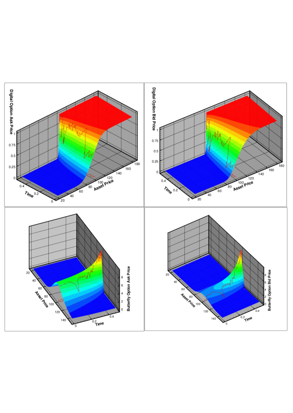
We use the numerical schemes constructed in Section 6 to compute the nonlinear PDE $(\ref{eq521})$ with the payoff function as initial condition and the boundary condition is $\phi(S_{\mbox{max}})=1$. We choose the grid as $\Delta s=1,\Delta t=0.0025$ and iterative tolerance$=10^{-6}$. We plot Fig. 1 the price trajectory on the ask (top left) price and bid (top right) price surfaces of the digital call option.

Example 7.2

Butterfly option under uncertain volatility.

The second example is a butterfly option with the payoff as follows

$$\phi(S_{T})=\max(S-K_{1},0)-2\max(S-(K_{1}+K_{2})/2,0)+\max(S-K_{2},0),$$

the boundary condition is $u^{a}(S_{\mbox{max}})=0,K_{1}=90$ and $K_{2}=110$. The other parameters used here are the same as that we used in example 1. The ask price (down left) and the bid price (down right) surfaces of the butterfly option are shown in Fig. 1.

Fig. 1 shows that the ask price trajectory is above the bid price trajectory for the both claims, and the ask (resp. bid) price dynamic keeps the monotone intervals and convex (resp. concave) intervals of the corresponding payoff function which verify the theoretical results we showed in Lemma 5.1.

Figure 1: Price trajectory on the ask (left top) and bid (right top) price surface of the digital option (up) and butterfly option (down).

References

• [1] Artzner, Ph., Delbaen F., Eber J. M. (1999) Coherent measures of risk, Mathematical Finance. 9, 73-88.
• [2] Avellaneda, M., Levy, A. and Par$\acute{\mbox{a}}$s, A. (1995) Pricing and Hedging Derivative Securities in Markets With Uncertain Volatilities, Appl. Math. Finance. 2, 73-88.
• [3] Barenblatt, G.I. (1978) Similarity, self-similarity and intermediate asympototics, Consultants Bureau, New York (there exists a revised second Russian edition, Leningrad Gidrometeoizdat, 1982).
• [4] Barenblatt, G.I. and Sivashinski, G.I. (1969) Self-similar solutions of the second kind in nonlinear filtration, Appl. Math. Mech. 33, 836-845(translated from Russian PMM, pages 861-870).
• [5] Barles, G. and Jakobsen, E.R. (2007) Error bounds for monotone approximation schemes for parabolic Hamilton-Jacobi-Bellman equations, Mathematics of Computation, 76, 1861-1893.
• [6] Bion-Nadal, J. (2009) Time consistent dynamic risk processes, Stochastic Processes and Their Applications, 119, 633-654.
• [7] Bion-Nadal, J. (2009) Bid-ask dynamic pricing in financial markets with transaction costs and liquidity risk, Journal of Mathematical Economics, 45, 738-750.
• [8] Chaumont, S. (2003) A strong comparision result for viscosity solutions to Hamilton-Jacobi-Bellman equations with Dirichlet condition on a non-smooth boundary, Acad. Sci. Paris, Ser. I 336.
• [9] Cherny, A., Madan, D.B. (2009) New measures for performance evaluation, The Review of Financial Studies, 22/7, 2571-2606.
• [10] Cherny, A., Madan, D.B. (2010) Illiquid market as a counterparty: an introduction to conic finance, International Journal of Theoretical and Applied Finance, 13/8, 1449-1177.
• [11] Crandall, M.G., Ishii, H., Lions, P.L. (1992) User’s guide to viscosity solutions of second order partial differential equations, Bull. Amer. Math. Soc. 27(1), 1-67.
• [12] Douglas, J.Jr., Russell, T.F. (1982) Numerical method for convection-dominated diffusion problem based on combing the method of characteristics with finite element or finite difference procedures, SIAM J. Numer. Anal., 19(5), 871-885.
• [13] Denis, L., Hu, M. and Peng, S. (2010) Function spaces and capacity related to a Sublinear Expectation: application to G-Brownian Motion Paths, Potential Analysis, 34, 139-161.
• [14] Eberlein, E., Madan, D.B., Pistorius, M., Schouotens, W., Yor, M. (2012) Two price economies in continuous time, Preprint (August, 2012), http://www.stochastik.uni-freiburg.de/eberlein/papers/TPECT1.pdf.
• [15] Epstein, L., Ji, Shaolin. (2011) Ambiguous volatility, possibility and utility in continuous time, arXiv:1103.1652v4.
• [16] Fleming, W., Soner, M. (1992) Controlled markov processes and viscosity solutions. Springer Verlag, New York.
• [17] Lyons, T. J. (1995) Uncertain volatility and the risk-free synthesis of derivatives, Appl. Math. Finance, 2, 117-133.
• [18] Madan, D.B. (2012) A two price theory of financial equilibrium with risk management implications, Ann Finance, 8, 489-505.
• [19] El Karoui, Peng, S., Quenez, M.-C. (1997) Backward stochastic differential equations in finance, Math. Finance. 7, 1-71.
• [20] Peng, S. (1992) A generalized dynamic programming principle and Hamilton-Jacobi-Bellman equation. Stochastics and Stochastic Reports, 38(2): 119-134.
• [21] Peng, S., (2004) Filtration Consistent Nonliear Expectations and Evaluations of Contingent Claims. Acta Mathematicae Applicatae Sinica, English Series, 20(2), 1-24.
• [22] Peng, S. (2005) G-Expectation, G-Brownian Motion and Related Stochastic Calculus of Ito Type, Stochastic Analysis and Applications, The Abel Symposium, 541-567.
• [23] Peng, S. (2008) Multi-dimensional G-Brownian Motion and Related stochastic Calculus under G-Expectation, Stochastic Processes and their Applications, 118, 2223-2253.
• [24] Peng, S. (2010) Nonlinear expectations and stochastic calculus under uncertainty - with robust central limit theorem and G-Brownian Motion, Preprint arXiv:1002.4546v1.
• [25] Song, Y. (2011) Some properties on G-evaluation and its applications to G-martingale decomposition, Science China Mathematics, 54(2), 287-300.
• [26] Varga, R.S. (2000) Matrix Iterative Analysis. Springer Verlag.