Analyses of turbulence in a wind tunnel by a multifractal theory for probability density functions

Abstract

The probability density functions (PDFs) for energy dissipation rates, created from time-series data of grid turbulence in a wind tunnel, are analyzed in a high precision by the theoretical formulae for PDFs within multifractal PDF theory which is constructed under the assumption that there are two main elements constituting fully developed turbulence, i.e., coherent and incoherent elements. The tail part of PDF, representing intermittent coherent motion, is determined by Tsallis-type PDF for singularity exponents essentially with one parameter with the help of new scaling relation whose validity is checked for the case of the grid turbulence. For the central part PDF representing both contributions from the coherent motion and the fluctuating incoherent motion surrounding the former, we introduced a trial function specified by three adjustable parameters which amazingly represent scaling behaviors in much wider area not restricted to the inertial range. From the investigation of the difference between two difference formulae approximating velocity time-derivative, it is revealed that the connection point between the central and tail parts of PDF extracted by theoretical analyses of PDFs is actually the boundary of the two kinds of instabilities associated respectively with coherent and incoherent elements.

Keywords: Multifractal, Fat tail, Intermittency, Turbulence, Energy dissipation rates

1 Introduction

There are several keystone works (Mandelbrot 1974, Parisi and Frisch 1985, Benzi et al1984, Halsey et al1986, Meneveau and Sreenivasan 1987, Nelkin 1990, Hosokawa 1991, Benzi et al1991, She and Leveque 1994, Dubrulle 1994, She Z-S and Waymire 1995, Arimitsu T and N 2000a, 2000b, 2001, 2002, Arimitsu N and T 2002, Biferale et al2004, Chevillard et al2006) providing the multifractal aspects for fully developed turbulence. Only a few works (Benzi et al1991, Arimitsu T and N 2001, 2002, Arimitsu N and T 2002, Biferale et al2004, Chevillard et al2006) analyze the probability density functions (PDFs) for physical quantities representing intermittent character. The other works deal with only the scaling property of the system, e.g., comparison of the scaling exponents of velocity structure function. Among the researches analyzing PDFs, multifractal probability density function theory (MPDFT) (Arimitsu T and N 2001, 2002, 2011, Arimitsu N and T 2002, 2011) provides the most precise analysis of the fat-tail PDFs. MPDFT is a statistical mechanical ensemble theory constructed by the authors (T.A. and N.A.) in order to analyze intermittent phenomena providing fat-tail PDFs.

To extract the intermittent character of the fully developed turbulence, it is necessary to have information of self-similar hierarchical structure of the system. This is realized by producing a series of PDFs for responsible singular quantities with different lengths

$$\ell_{n}=\ell_{0}\delta^{-n},\quad\delta>1\quad({n}=0,1,2,\cdots)$$ (1)

that characterize the regions in which the physical quantities are coarse-grained. The value for $\delta$ is chosen freely by observers. Let us assume that the self-similar structure of fully developed turbulence is such that the choice of $\delta$ should not affect the theoretical estimation of the values for the fundamental quantities characterizing the turbulent system under consideration. A&A model within the framework of MPDFT itself tells us that this requirement is satisfied if the scaling relation has the form (Arimitsu T and N 2011, Arimitsu N and T 2011)

$$\ln 2/(1-q)\ln\delta=1/\alpha_{-}-1/\alpha_{+}.$$ (2)

Here, $q$ is the index associated with the Rényi entropy (Rényi 1961) or with the Havrda-Charvat and Tsallis (HCT) entropy (Havrda and Charvat 1967, Tsallis 1988); $\alpha_{\pm}$ are zeros of the multifractal spectrum $f(\alpha)$ (see below in section 2). The multifractal spectrum is uniquely related to the PDF for $\alpha$ (see (4) below). The PDF of $\alpha$ is related to the tail part of PDFs within MPDFT for those quantities revealing intermittent behavior whose singularity exponents can have values $\alpha<1$, e.g., the energy dissipation rates, through the variable transformation between $\alpha$ and the physical quantities (see (3) below for the case of the energy dissipation rates $\varepsilon_{n}$). With the new scaling relation (2), observables have come to depend on the parameter $\delta$ only in the combination $(1-q)\ln\delta$. The difference in $\delta$ is absorbed in the entropy index $q$.

In the preceding papers, we analyzed PDFs for energy transfer rates (Arimitsu T and N 2011) and PDFs for energy dissipation rates (Arimitsu N and T 2011), which are given in figure 11 of Aoyama et al(2005), with the help of the new scaling relation, and checked the independence of the PDFs from $\delta$. It was found that the adjustable parameters for the central part PDF provide us with $\delta$-independent scaling behaviors as functions of $r/\eta$, and that the scaling properties are satisfied in much wider region not restricted to inside of the inertial range. However, the number of data points used in drawing the PDFs in figure 11 of Aoyama et al(2005) is not enough, especially, for the precise analyses of the central part of the PDFs performed in Arimitsu T and N (2011) and Arimitsu N and T (2011). Therefore, we will perform, as one of the aims of the present paper, the same analyses, which were done for DNS, with the help of PDFs created from wind tunnel turbulence with a higher enough resolution in order to make sure if the characteristics discovered previously with rather poor resolution at the central part are correct or not. Since we have the raw time-series data taken from wind tunnel turbulence, we can create PDFs for energy dissipation rates with enough resolutions fit to our needs.

In this paper, we analyze the PDFs for energy dissipation rates extracted out from the time series of the velocity field of a fully developed turbulence which were observed by one of the authors (H.M.) in his experiment conducted in a wind tunnel (Mouri et al2008). In section 2, we present the formulae of theoretical PDFs within A&A model which are necessary in the following sections for the analyses of PDFs obtained from the experimental turbulence. In section 3, we analyze the observed PDFs for energy dissipation rates in a high precision with the theoretical PDF within A&A model of MPDFT, and verify the proposed assumption related to the magnification $\delta$. In section 4, in order to see what information we can extract out from the time-series data, we compare two different PDFs for energy dissipation rates created from the time series data with different approximation for temporal derivative. We may learn from this how to treat the central part of PDFs to derive the information of incoherent fluctuating motion around the coherent turbulent motion. Summary and discussion are provided in section 5.

2 Singularity exponent and PDFs for energy dissipation rates

MPDFT is constructed under the assumption, following Parisi and Frisch (1985), that for high Reynolds number the singularities distribute themselves in a multifractal way in real physical space. The singularities stem from the invariance of the Navier-Stokes (N-S) equation for an incompressible fluid under the scale transformation ${\vec{x}}\rightarrow{\vec{x}}^{\prime}=\lambda{\vec{x}}$, accompanied by the scale changes ${\vec{u}}\rightarrow{\vec{u}}^{\prime}=\lambda^{\alpha/3}{\vec{u}}$ in velocity field, $t\rightarrow t^{\prime}=\lambda^{1-\alpha/3}t$ in time and $p\rightarrow p^{\prime}=\lambda^{2\alpha/3}p$ in pressure with an arbitrary real number $\alpha$, in the limit of large Reynolds number, i.e., the contribution from the dissipation term in N-S equation, which is proportional to the kinematic viscosity $\nu$, is negligibly small compared with the convection term. In treating an actual turbulent system, however, the value $\nu$ is fixed to a finite value unique to the material of fluid prepared for an experiment. We should keep in mind that the dissipation term can become effective depending on the region under consideration, since the term breaking the invariance does exist, i.e., non-zero (see the discussion in the following).

The invariance under the scale transformation leads to the scaling property

$$\varepsilon_{n}/\epsilon=\left(\ell_{n}/\ell_{0}\right)^{\alpha-1}$$ (3)

for the energy dissipation rate $\varepsilon_{n}$ averaged in the regions with diameter $\ell_{n}$. Here, we put $\varepsilon_{0}=\epsilon$ whose value is assumed to be constant. The energy dissipation rate becomes singular for $\alpha<1$, i.e., $\lim_{n\rightarrow\infty}\varepsilon_{n}=\lim_{n\rightarrow\infty}\ell_{n}^{\alpha-1}\rightarrow\infty$. The degree of singularity is specified by the singularity exponent $\alpha$ (Parisi and Frisch 1985).

Let us consider $\alpha$ to be a stochastic variable whose PDF $P^{(n)}(\alpha)$ is given by the Rényi or HCT type function (Arimitsu T and N 2000a, 2000b, 2001, 2002, 2011, Arimitsu N and T 2002, 2011):

$$P^{(n)}(\alpha)\propto\left[1-(\alpha-\alpha_{0})^{2}/({\it\Delta}\alpha)^{2}\right]^{n/(1-q)}$$ (4)

with ${\it\Delta}\alpha=\left[2X/(1-q)\ln\delta\right]^{1/2}$. The domain of $\alpha$ is $\alpha_{\rm min}\leq\alpha\leq\alpha_{\rm max}$ with $\alpha_{\rm min}$ and $\alpha_{\rm max}$ being given by $\alpha_{\rm min/max}=\alpha_{0}\mp{\it\Delta}\alpha$. $q$ is the entropy index. From (4), we have for $n\gg 1$ the expression of the multifractal spectrum

$$f(\alpha)=1+\ln\left[1-(\alpha-\alpha_{0})^{2}/({\it\Delta}\alpha)^{2}\right]/(1-q)\ln\delta.$$ (5)

The independence of $f(\alpha)$ from $n$ is interpreted as a manifestation of the existence of self-similar hierarchical structure responsible for the intermittent fluid motion of turbulence.

The three parameters $\alpha_{0}$, $X$ and $q$ appeared in $P^{(n)}(\alpha)$ are determined as the functions of the intermittency exponent $\mu$ with the help of the three conditions. One is the energy conservation law $\langle\varepsilon_{n}\rangle=\epsilon$. Another is the definition of the intermittency exponent $\mu$, i.e., $\langle(\varepsilon_{n}/\epsilon)^{2}\rangle=(\ell_{n}/\ell_{0})^{-\mu}$. The last condition is the scaling relation (2) with $\alpha_{\pm}$ being the solution of $f(\alpha_{\pm})=0$, which is a generalization of the one introduced by Tsallis and his coworkers (Costa et al1998, Lyra and Tsallis 1998) to which (2) reduces when $\delta=2$. Here, the average $\langle\cdots\rangle$ is taken with $P^{(n)}(\alpha)$. The parameter $q$ is determined, altogether with $\alpha_{0}$ and $X$, as a function of $\mu$ only in the combination $(1-q)\ln\delta$. The difference in $\delta$ is absorbed into the entropy index $q$, therefore changing the zooming rate $\delta$ may result in picking up the different hierarchy, containing the entropy specified by the index $q$, out of self-similar structure of turbulence. As the parameters are dependent on $q$ only in the combination $(1-q)\ln\delta$, we are naturally led to the replacement of $n$ in the expression of $P^{(n)}(\alpha)$ in (4) with $n=\tilde{n}/\ln\delta$. If $\tilde{n}$ does not depend on $\delta$, $P^{(n)}(\alpha)$ becomes also independent of $\delta$. Note that, with the new number $\tilde{n}$, $\ell_{n}$ introduced in (1) reduces to

$$\ell_{n}=\ell_{0}\mbox{e}^{-\tilde{n}}.$$ (6)

MPDFT provides us with a systematic framework to make a connection between the PDF $P^{(n)}(\alpha)$ of the singularity exponent $\alpha$ and the PDF of the observed quantity such as the energy dissipation rate representing intermittent singular behavior in its time-evolution. The element of fluid motion specified by the singularity exponent satisfying $\alpha<1$ takes care of the intermittent large (singular) spikes observed in the time-evolution of energy dissipation rate, and contributes to the tail part of PDF for energy dissipation rates (see figure 1 (a) and (b)). This element is directly related to a coherent hierarchical structure such as the multi-scale Cantor set characterized by the multifractal spectrum $f(\alpha)$. Therefore, the fluid motion controlled by this element is referred to as a coherent motion. There is another element of fluid motion due to the symmetry breaking term, i.e., the dissipation term in N-S equation, which produces fluctuation of fluid surrounding the coherent turbulent motion. This element contributes mainly to the central part of PDF (see figure 1 (a) and (b)). The fluid motion provided by this element is referred to as an in-coherent motion. Note that the central part of the PDF is constituted of two elements, i.e., the in-coherent and coherent motions.

Figure 1: Two kinds of divisions of PDF $\Pi_{3}^{(n)}(\varepsilon_{n})$. One into $\Pi^{(n)}_{3,{\rm S}}(\varepsilon_{n})$ and ${\it\Delta}\Pi_{3}^{(n)}(\varepsilon_{n})$ are given on (a) linear and (b) log scale in the vertical axes. The other into $\hat{\Pi}_{3,{\rm cr}}^{(n)}(\xi_{n})$ and $\hat{\Pi}_{3,{\rm tl}}^{(n)}(\xi_{n})$ is given in (c) on log scale. The open circles represent an experimental PDF for energy dissipation rates. The contribution of ${\it\Delta}\Pi_{3}^{(n)}(\varepsilon_{n})$ to the tail part $\hat{\Pi}_{3,{\rm tl}}^{(n)}(\xi_{n})$ is negligibly small.

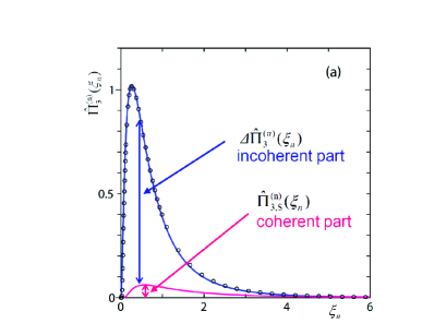
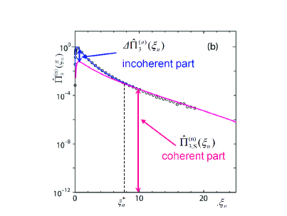
Based on the above consideration, we assume that the probability $\Pi^{(n)}_{3}(\varepsilon_{n})d\varepsilon_{n}$ can be, generally, divided into two parts as

$$\Pi_{3}^{(n)}(\varepsilon_{n})d\varepsilon_{n}=\Pi^{(n)}_{3,{\rm S}}(\varepsilon_{n})d\varepsilon_{n}+{\it\Delta}\Pi_{3}^{(n)}(\varepsilon_{n})d\varepsilon_{n}$$ (7)

(see figure 1 (a) and (b)). The first term describes the coherent motion, i.e., the contribution from the abnormal part of the physical quantity $\varepsilon_{n}$ due to the fact that its singularities distribute themselves multifractal way in real space. This is the part representing a coherent turbulent motion given in the limit $\nu\rightarrow 0$ but is not equal to zero ($\nu\neq 0$). The second term represents the contribution from the incoherent fluctuating motion. The normalization of PDF is specified by $\int_{0}^{\infty}d\varepsilon_{n}\Pi_{3}^{(n)}(\varepsilon_{n})=1$. We assume that the coherent contribution is given by (Arimitsu T and N 2001) $\Pi^{(n)}_{3,{\rm S}}(\varepsilon_{n})d\varepsilon_{n}=\bar{\Pi}_{3,{\rm S}}^{(n)}P^{(n)}(\alpha)d\alpha$ with the variable transformation (3). For the expression of $\bar{\Pi}_{3,{\rm S}}^{(n)}$, see Arimitsu N and T (2011).

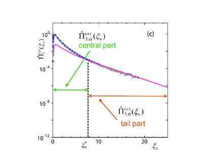
Let us introduce another division of the PDF (see figure 1 (c)), i.e.,

$$\hat{\Pi}_{3}^{(n)}(\xi_{n})=\hat{\Pi}_{3,{\rm cr}}^{(n)}(\xi_{n})+\hat{\Pi}_{3,{\rm tl}}^{(n)}(\xi_{n}),$$ (8)

where $\hat{\Pi}_{3}^{(n)}(\xi_{n})$ is introduced by the relation $\hat{\Pi}_{3}^{(n)}(\xi_{n})d\xi_{n}=\Pi_{3}^{(n)}(\varepsilon_{n})d\varepsilon_{n}$ with the variable transformation $\xi_{n}=\varepsilon_{n}/\langle\!\langle\varepsilon_{n}^{2}\rangle\!\rangle_{\rm c}^{1/2}$ where the cumulant average $\langle\!\langle\cdots\rangle\!\rangle_{\rm c}$ is taken with the PDF $\Pi_{3}^{(n)}(\varepsilon_{n})$. The two parts of the PDF, the tail part $\hat{\Pi}_{3,{\rm tl}}^{(n)}(\xi_{n})$ and the central part $\hat{\Pi}_{3,{\rm cr}}^{(n)}(\xi_{n})$, are connected at $\xi_{n}=\xi_{n}^{*}$ under the conditions that they have the common value and the common log-slope there. Note that $\xi_{n}^{*}$ is related to $\varepsilon_{n}^{*}$ by $\xi_{n}^{*}=\varepsilon_{n}^{*}/\langle\!\langle\varepsilon_{n}^{2}\rangle\!\rangle_{\rm c}^{1/2}$ and to $\alpha^{*}$ by (3). The value of $\alpha^{*}$ is determined for each PDF as an adjusting parameter in the analysis of PDFs obtained by ordinary or numerical experiments.

When one creates a PDF from the time-evolution data for microscopic energy dissipation rate, he puts each realization into an appropriate bin according to the value $\varepsilon_{n}$ which is obtained by averaging the microscopic energy dissipation rates in each time interval corresponding to the length $\ell_{n}$. For larger $\varepsilon_{n}$ values belonging to the tail part domain of the PDF, most of the realizations in a bin at the interval $\varepsilon_{n}\sim\varepsilon_{n}+d\varepsilon_{n}$ come from the time interval containing at least one intermittently large spike (singular spike) of microscopic energy dissipation rates. The bin may have negligibly small proportion of the number of realizations coming from those intervals with only fluctuations compared to the number of realizations with at least one singular spike. On the other hand, for smaller $\varepsilon_{n}$ values belonging to the central part PDF domain, the number of realizations coming from the time intervals containing singular spikes with smaller heights is about the same order as the number of realizations from the time intervals containing only fluctuations, since the height of singular spikes contributing to this bin must be about the same height as fluctuations.

Under the above interpretation, it may be reasonable to assume that, for the tail part of PDF $\hat{\Pi}_{3,{\rm tl}}^{(n)}(\xi_{n})$, the contribution from the first term $\Pi_{3,{\rm S}}^{(n)}(\varepsilon_{n})$ in (7) to the intermittent rare events dominates, and the contribution from the second term ${\it\Delta}\Pi_{3}^{(n)}(\varepsilon_{n})$ to the events is negligible, i.e.,

$$\hat{\Pi}_{3,{\rm tl}}^{(n)}(\xi_{n})\ d\xi_{n}=\Pi^{(n)}_{3,\rm S}(\varepsilon_{n})\ d\varepsilon_{n}$$ (9)

for $\xi_{n}^{*}\leq\xi_{n}$. For $0\leq\xi_{n}\leq\xi_{n}^{*}$, as there is no theory for the central part of PDF $\hat{\Pi}_{3,{\rm cr}}^{(n)}(\xi_{n})$ at present, we put

$$\hat{\Pi}_{3,{\rm cr}}^{(n)}(\xi_{n})d\xi_{n} = \bar{\Pi}_{3}^{(n)}\mbox{e}^{-[g_{3}(\xi_{n})-g_{3}(\xi_{n}^{*})]}\ \left(\ell_{n}/\ell_{0}\right)^{1-f(\alpha^{*})}\ \left(\bar{\xi}_{n}/\xi_{n}^{*}\right)d\xi_{n}$$ (10)

with $\bar{\Pi}_{3}^{(n)}=\bar{\Pi}_{3,S}^{(n)}\sqrt{|f^{\prime\prime}(\alpha_{0})|/2\pi|\ln(\ell_{n}/\ell_{0})|}/\bar{\xi}_{n}$ and a trial function of the Tsallis-type

$$\mbox{e}^{-g_{3}(\xi_{n})}=\left(\xi_{n}/\xi_{n}^{*}\right)^{\theta-1}$$ (11)

$$\times\left\{1-\left(1-q^{\prime}\right)\left[\theta+f^{\prime}(\alpha^{*})\right]\left[\left(\xi_{n}/\xi_{n}^{*}\right)^{w_{3}}-1\right]/w_{3}\right\}^{1/(1-q^{\prime})}$$

containing minimal number of adjustable parameters, i.e., $q^{\prime}$, $\theta$ and $w_{3}$. The parameter $w_{3}$ is adjusted by the property of the experimental PDFs around the connection point; $q^{\prime}$ is the entropy index different from $q$ in (4); $\theta$ is determined by the property of PDF near $\xi_{n}=0$. For the expression of $\bar{\xi}_{n}$, see Arimitsu N and T (2011). The contribution to $\hat{\Pi}_{3,{\rm cr}}^{(n)}(\xi_{n})$ comes both from coherent and incoherent motions (see figure 1).

The reason why we chose the trial function (11) for the central part PDF is because it is a natural generalization of the $\chi$-square distribution function for the variable $y_{n}=(\xi_{n}/\xi_{n}^{*})^{w_{3}}$. The observed value of $q^{\prime}$ is in the range $1.03\leq q^{\prime}\leq 1.09$ (see table 2). Note that in the limit $q^{\prime}\rightarrow 1$ the trial function reduces to the $\chi$-square distribution function for $y_{n}$. The quantity $(\theta+w_{3}-1)/w_{3}$ provides us with an estimate for the number of independent degrees of freedom for the dynamics contributing to the central part of PDF.

3 Verification of assumptions through the analyses of experimental PDFs

3.1 Experimental setup and extraction of PDFs

By means of the theoretical formula within MPDFT summarized in the last section, we analyze PDFs of energy dissipation rates created from the time series data (Mouri et al2008) for the turbulence produced by a grid in a wind tunnel (see table 1). Measurements are performed by a hot-wire anemometer with a crossed-wire probe placed on the centerline of the tunnel at $4$ m downstream from the grid. It is expected that turbulence around the probe is homogeneous in both stream-wise and span-wise directions, as the cross-section $16$ cm $\times$ $16$ cm of each open square surrounded by the rods constituting the grid is small enough compared with the cross-section $3$ m $\times$ 2 m of the wind tunnel. The cross section of a rod is $4$ cm $\times$ $4$ cm. We also expect that the turbulence around the probe is isotropic even for larger scales since the values of RMS one-point velocity fluctuations for span-wise and stream-wise components are almost equal (see table 1). There are still possible pitfalls about the assumption of isotropy (Biferale and Procaccia 2005) because of the difference of values between the averaged energy dissipation rates estimated with the span-wise velocity component $v$, i.e., $15\nu\langle\!\langle(\partial v/\partial x)^{2}\rangle\!\rangle/2=\langle\!\langle\varepsilon\rangle\!\rangle=7.98$ m² sec^-3, and the one estimated with the stream-wise velocity fluctuation $u$, i.e., $15\nu\langle\!\langle(\partial u/\partial x)^{2}\rangle\!\rangle=8.58$ m² sec^-3 (Mouri et al2008). However, as the difference is less than 10 %, we expect that anisotropy, even if it exists, may not affect the following analyses seriously.

Table 1: Parameters of the grid turbulence in a wind tunnel (Mouri et al2008). The inertial range is determined as the region where the second moment of the velocity differences for longitudinal component scales with the exponent $2/3$ with respect to the distance between the positions of two velocities used to derive the velocity difference.

Quantity	Value
Microscale Reynolds number Reλ	409
Kolmogorov length $\eta$	$0.138$ mm
Kinematic viscosity $\nu$	$1.42\times 10^{-5}$ m2 sec-1
Mean velocity of downstream wind $U$	21.16 m sec-1
Mean energy dissipation rate $\langle\!\langle\varepsilon\rangle\!\rangle=15\nu\langle\!\langle(\partial v/\partial x)^{2}\rangle\!\rangle/2$	7.98 m2 sec-3
Correlation length of longitudinal velocity	$17.9$ cm
Inertial range	$50\lesssim r/\eta\lesssim 150$
RMS of span-wise velocity fluctuations $\langle\!\langle v^{2}\rangle\!\rangle^{1/2}$	1.06 m sec-1
RMS of stream-wise velocity fluctuations $\langle\!\langle u^{2}\rangle\!\rangle^{1/2}$	1.10 m sec-1
Sampling interval ${\it\Delta}t$	$1.43\times 10^{-5}$ sec
Number of data points	$4\times 10^{8}$

Assuming isotropy of the grid turbulence, we adopted the surrogate $15\nu(\partial v/\partial x)^{2}/2=15\nu(\partial v/\partial t)^{2}/2U^{2}$ for the energy dissipation rate (Cleve et al2003, Mouri et al2008) with the mean velocity $U$ of downstream wind (see table 1) where $x$-axis is chosen to the direction of the mean flow in a wind tunnel and $v$ is the span-wise velocity component. Here, we used Taylor’s frozen hypothesis in replacing the variable from time $t$ to space $x$ (see Mouri et al(2008) for detail). For the estimation of $\partial v/\partial t$, we use here the difference formula

$$\partial v/\partial t\simeq{\it\Delta}^{(3)}v/{\it\Delta}t = \left\{8\ [v(t+{\it\Delta}t)-v(t-{\it\Delta}t)]\right.$$ (12)

$$\left.-[v(t+2{\it\Delta}t)-v(t-2{\it\Delta}t)]\right\}/12{\it\Delta}t$$

where ${\it\Delta}t$ is the sampling interval observing velocity (see table 1). With this formula, we can have a better estimate of the velocity time derivative by means of ${\it\Delta}^{(3)}v/{\it\Delta}t$ without contamination up to the term of ${\cal O}({\it\Delta}t)^{3}$. We represent the local energy dissipation rates derived from (12) by the symbol $\varepsilon$, i.e., $\varepsilon=15\nu({\it\Delta}^{(3)}v/{\it\Delta}t)^{2}/2U^{2}$.

In creating the experimental PDFs for energy dissipation rates, $4\times 10^{8}$ data points are put into $2\times 10^{4}$ bins along the $\xi_{n}$ axis. We discarded those bins containing the number of data points less than 25. Note that the average number of data points per bin is $2\times 10^{4}$. In drawing the created PDFs for energy dissipation rates, not all the bins but every $10^{2}$ bins are plotted for better visibility. The experimental PDF in the region near the right-most end points are scattered because of the lower statistics due to smaller number of data points in the bins located there (see figure 2 (a) and figure 4 (a)).

3.2 Analyses of experimental PDFs

The experimental PDF is analyzed with the help of the theoretical formula for PDF by the following procedure: (i) Pick up three experimental PDFs with consecutive $r$ values, say, $r_{1}$, $r_{2}=r_{1}\delta$ and $r_{3}=r_{1}\delta^{2}$. (ii) With a trial $\mu$ value, analyze each of the three experimental PDFs to find out tentative but the best values $q^{\prime}$, $w_{3}$, $\theta$, $\alpha^{*}$ and $n_{i}=\ln(r_{i}/\ell_{0})/\ln\delta$ ($i=1$, 2, 3) for the theoretical PDF. (iii) Check if the differences $n_{3}-n_{2}$ and $n_{2}-n_{1}$ are close to 1 or not. (iv) If not, change $\mu$ value, and repeat the processes (ii) and (iii) until one arrives at the set of best fit parameters under the condition $n_{3}-n_{2}=n_{2}-n_{1}\simeq 1$ within a settled accuracy. (v) With thus determined common $\mu$ value, determine the best fit values $q^{\prime}$, $w_{3}$, $\theta$ and $\alpha^{*}$ for each of other PDFs which are not picked out for the above processes (i) to (iv). One notices that $n_{i}-n_{i-1}\simeq 1$ are satisfied automatically for every PDFs created from the experiment.

Figure 2: PDFs of energy dissipation rates for $\delta=3$ on (a) log and (b) linear scale in the vertical axes. For better visibility, each PDF is shifted by $-2$ unit along the vertical axis in (a) and by $-0.4$ unit along the vertical axis in (b). Closed circles are the experimental PDFs for $r/\eta=21.9$, $65.7$, $197$ and $591$ from the smallest value (top) to the largest value (bottom) where $r$ corresponds to $\ell_{n}$. Solid lines represent the curves given by the present theory with parameters listed in table 2 (a).

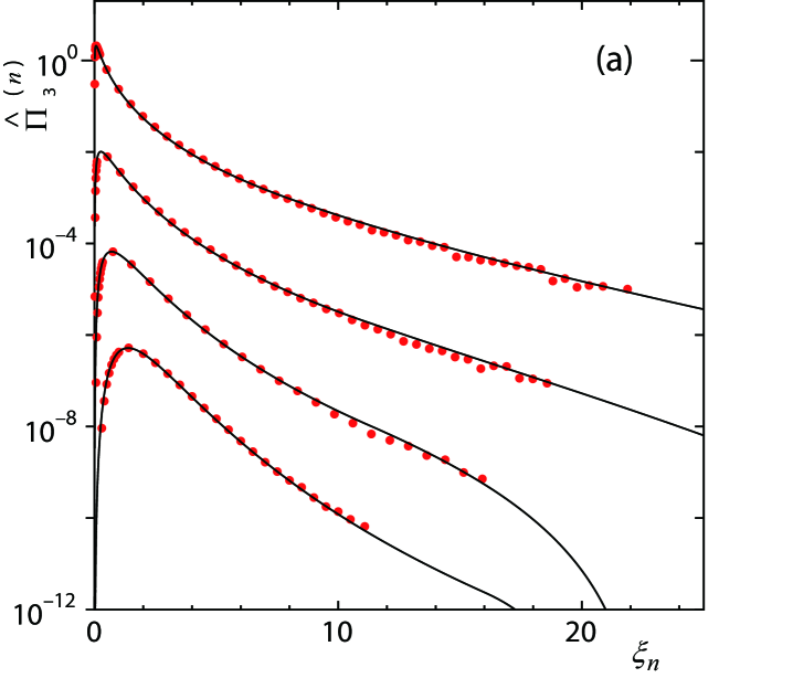
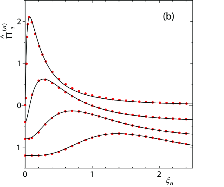
The PDFs of energy dissipation rates are analyzed in figure 2 for the magnification $\delta=3$ on (a) log and (b) linear scale in the vertical axes. For better visibility, each PDF is shifted by appropriate unit along the vertical axis. Closed circles are the experimental data points for PDFs for the cases $r/\eta=21.9$, $65.7$, $197$ and $591$ from the smallest value (top) to the largest value (bottom) where $r$ corresponds to $\ell_{n}$. Solid lines represent the theoretical PDFs given by (8) with (9) and (10). The parameters necessary for the theoretical PDF of A&A model are determined as $(1-q)\ln\delta=0.393$, $\alpha_{0}=1.15$ and $X=0.310$, which turn out to be independent of $\delta$. Other parameters are listed in table 2 (a) and table 3 (a). We performed the same analyses for other magnifications, $\delta=2$ and 5, and found that the extracted value $\mu=0.260$ for the intermittency exponent is common to three cases in which PDFs are created with the different values of magnification, i.e., $\delta=2$, 3, 5. It means that, within the analysis of the energy dissipation rates, the turbulent system under consideration is characterized by a unique $\mu$ value as it should be.

Table 2: Parameters of PDFs created by (a) the formula (12) and (b) the formula (13). For both cases, $\mu=0.260$ ($(1-q)\ln\delta=0.393$, $\alpha_{0}=1.15$, $X=0.310$) giving $q=0.642$.

	(a)					(b)
$r/\eta$	$n$	$\tilde{n}$	$q^{\prime}$	$w_{3}$	$\theta$	$n$	$\tilde{n}$	$q^{\prime}$	$w_{3}$	$\theta$
6.57	5.50	6.04	1.03	0.250	2.10	5.20	5.71	1.03	0.250	3.50
21.9	4.00	4.39	1.02	0.250	3.50	4.00	4.39	1.04	0.380	5.30
65.7	3.00	3.30	1.05	0.490	4.10	3.00	3.30	1.04	0.450	5.00
197	1.60	1.76	1.06	0.780	4.50	2.00	2.20	1.07	0.750	6.00
591	0.60	0.416	1.09	1.25	5.80	0.580	0.637	1.09	1.24	6.20

Table 3: Connection points between the central and the tail part PDFs created by (a) the formula (12) and (b) the formula (13). $\langle\!\langle\varepsilon\rangle\!\rangle=7.98$ m² sec^-3.

	(a)			(b)
$r/\eta$	$\alpha^{*}$	$\varepsilon_{n}^{*}/\langle\!\langle\varepsilon\rangle\!\rangle$	$\xi_{n}^{*}$	$\alpha^{*}$	$\varepsilon_{n}^{*}/\langle\!\langle\varepsilon\rangle\!\rangle$	$\xi_{n}^{*}$
6.57	0.750	4.53	3.30	0.750	4.17	3.56
21.9	0.700	3.74	3.56	0.550	7.22	5.24
65.7	0.500	5.20	5.25	0.500	5.20	6.25
197	0.280	3.54	13.6	0.300	4.66	13.2
591	0.180	1.72	16.0	0.180	1.69	15.3

Figure 3: $r/\eta$ ($=\ell_{n}/\eta$) dependence of (a) $\tilde{n}$, (b) $\alpha^{*}$ and (c) $\theta$. In (a), the data points extracted by the present analysis via (12) are plotted by closed circles for $\delta=2$, by closed squares for $\delta=3$, by closed triangles for $\delta=5$, whereas those extracted by the DNS analysis (Arimitsu N and T 2011) are plotted by symbols nabla for $\delta=2^{1/4}$, by times for $\delta=2^{1/2}$, by pluses for $\delta=2$. The empirical formula for the present (DNS) analysis is given by $\tilde{n}=-2.39\log_{10}(r/\eta)+7.31$ ($\tilde{n}=-2.33\log_{10}(r/\eta)+8.74$). In (b) and (c), the data points extracted by the present analyses via (12) (via (13)) are plotted by closed (open) circles for $\delta=2$, by closed (open) squares for $\delta=3$, by closed (open) triangles for $\delta=5$. Solid (dashed) lines are the empirical formulae (b) $\alpha^{*}=-0.326\log_{10}(r/\eta)+1.05$ ($\alpha^{*}=-0.285\log_{10}(r/\eta)+0.966$) and (c) $\theta=1.83\log_{10}(r/\eta)+0.460$ ($\theta=1.32\log_{10}(r/\eta)+2.70$). The empirical formulae are obtained by using all the data points for different values of $\delta$. The inertial range for the present (DNS) analysis is the region between the vertical dash-dotted (dotted) lines.

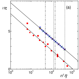
The dependence of $\tilde{n}$ on $r/\eta$ ($=\ell_{n}/\eta$) for the present analysis with the series of PDFs derived through (12) is given in figure 3 (a) by closed circles for $\delta=2$, by closed squares for $\delta=3$ and by closed triangles for $\delta=5$. The empirical formula for $\tilde{n}$ obtained by making use of all the data points for $\delta=2$, 3 and 5 with the method of least squares has the expression $\tilde{n}=-1.03\ln(r/\eta)+7.31$ which is drawn by a solid line (lower line in the figure). This proves the correctness of the assumption that the fundamental quantities of turbulence are independent of $\delta$. We also include in the figure, for comparison, the data points of $\tilde{n}$ for $4096^{3}$ DNS taken from figure 4 in Arimitsu N and T (2011) and the empirical formula $\tilde{n}=-1.01\ln(r/\eta)+8.74$ (upper solid line) derived with the data points by the method of least squares. For the DNS, $\mu=0.345$ (Arimitsu N and T 2011). How much $\tilde{n}$ data points are scattered from the empirical formula (see figure 3 (a)) and also from the theoretical formula (6) with $\ell_{n}=r$ provides us with a measure how much we perform appropriate extraction of parameters. The data points of $\tilde{n}$ for the turbulence in the wind tunnel are scattered more compared with those for the turbulence in $4096^{3}$ DNS, as the time-series raw data from wind tunnel include indispensable measurement errors associated with readout processes, e.g., mainly, electrical noises.

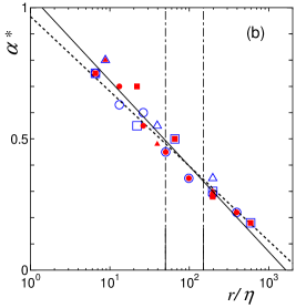
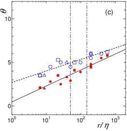
The $r/\eta$ ($=\ell_{n}/\eta$) dependences of $\alpha^{*}$ and $\theta$ are given, respectively, in figure 3 (b) and (c) by closed circles for $\delta=2$, by closed squares for $\delta=3$ and by closed triangles for $\delta=5$, which are extracted from the series of PDFs derived through (12). The solid line in each figure, (b) and (c), represents an empirical formula obtained from all the data points for $\delta=2$, 3 and 5 by the method of least squares. These figures prove again the correctness of the assumption that the fundamental quantities of turbulence are independent of $\delta$. The value of $q^{\prime}$ is found to be about $q^{\prime}=1.05$ (see table 2 (a)). We found that $w_{3}$ is also independent of $\delta$ and has a common line $\log_{10}w_{3}=0.372\log_{10}(r/\eta)+\log_{10}0.112$. Note that the empirical formulae for $\tilde{n}$, $\alpha^{*}$ and $\theta$ is effective only for the region $r/\eta\gtrsim 2$ since $\theta$ should satisfy $\theta>1$ (see figure 3 (c)). We observe that the parameters $q^{\prime}$, $\theta$, $w_{3}$ for the central part PDF and the connection point $\alpha^{*}$ have scaling behaviors in much wider region not restricted to inside of the inertial range.

4 Comparison of PDFs produced with full and less contaminations

In this section, we analyze the PDFs for the energy dissipation rates derived from the time-series data with the difference formula

$$\partial v/\partial t\simeq{\it\Delta}^{(0)}v/{\it\Delta}t=\left[v(t+{\it\Delta}t)-v(t)\right]/{\it\Delta}t$$ (13)

in order to study what difference comes out compared with the PDFs analyzed in section 3 which is derived by means of the difference formula (12). Note that the formula (13) estimates the values of velocity time derivative with ${\it\Delta}^{(0)}v/{\it\Delta}t$ which may contain full contamination, i.e., from the 1st order term with respect to ${\it\Delta}t$. We introduce the symbol $\varepsilon^{(0)}$ for the local energy dissipation rates derived from (13), i.e., $\varepsilon^{(0)}=15\nu({\it\Delta}^{(0)}v/{\it\Delta}t)^{2}/2U^{2}$. In creating the experimental PDFs for the energy dissipation rates, we took the same procedure as used in section 3.

Figure 4: Comparison of PDFs for energy dissipation rates $\Pi_{3}^{(n)}(\varepsilon/\langle\!\langle\varepsilon\rangle\!\rangle)$ and $\Pi_{3}^{(n)}(\varepsilon^{(0)}/\langle\!\langle\varepsilon\rangle\!\rangle)$ created, respectively, with the formulae (12) and (13). In (a) and (d)–(f), closed (open) circles and full (dashed) lines are, respectively, the experimental and theoretical PDFs for $\Pi_{3}^{(n)}(\varepsilon/\langle\!\langle\varepsilon\rangle\!\rangle)$ ($\Pi_{3}^{(n)}(\varepsilon^{(0)}/\langle\!\langle\varepsilon\rangle\!\rangle)$) with $\mu=0.260$. PDFs in (a) represent for the cases $r/\eta=6.57$ (top), $21.9$ (middle) and $65.7$ (bottom), shifted by $-2$ unit along the vertical axis for better visibility. The magnification of the central part PDFs for each $r$ ($=\ell_{n}$) is given in (d)–(f). The relative difference $\Delta_{n}=[\Pi_{3}^{(n)}(\varepsilon^{(0)}/\langle\!\langle\varepsilon\rangle\!\rangle)-\Pi_{3}^{(n)}(\varepsilon/\langle\!\langle\varepsilon\rangle\!\rangle)]/\Pi_{3}^{(n)}(\varepsilon/\langle\!\langle\varepsilon\rangle\!\rangle)$ is given for (b) $r/\eta=6.57$ and (c) 65.7, in which closed circles (full lines) are experimental (theoretical) $\Delta_{n}$. The error bar is the standard deviation of 100 hidden (not appeared in the figures) data points for $\Delta_{n}$ which locate between the adjacent data points for $\Delta_{n}$ appeared in the figures. The shown error bars are thinned out. Note that (a) and (b)–(f) are, respectively, drawn on log and linear scale in the vertical axes.

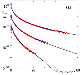
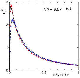
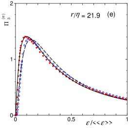
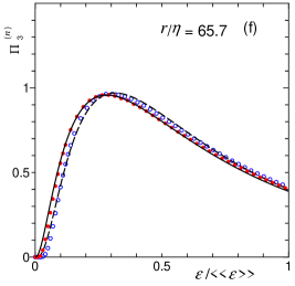
We compare, in figures 4 (a) and (d)–(f), the PDFs of energy dissipation rates $\Pi_{3}^{(n)}(\varepsilon/\langle\!\langle\varepsilon\rangle\!\rangle)$ and $\Pi_{3}^{(n)}(\varepsilon^{(0)}/\langle\!\langle\varepsilon\rangle\!\rangle)$ which are created, respectively, with the help of formulae (12) and (13). Note that the arguments for every PDFs are scaled by $\langle\!\langle\varepsilon\rangle\!\rangle$ which does not depend on $r$ ($=\ell_{n}$). In figure 4 (a) each PDF is displayed on log scale in vertical axis for the cases $r/\eta=6.57$ (top), $21.9$ (middle) and $65.7$ (bottom), which are shifted by $-2$ unit along the vertical axis for better visibility. The magnification of their central part PDFs are displayed in figures 4 (d) $r/\eta=6.57$, (e) $21.9$ and (f) $65.7$ on linear scale in vertical axis. The closed (open) circles and the full (dashed) lines are, respectively, the experimental and theoretical PDFs for $\Pi_{3}^{(n)}(\varepsilon/\langle\!\langle\varepsilon\rangle\!\rangle)$ ($\Pi_{3}^{(n)}(\varepsilon^{(0)}/\langle\!\langle\varepsilon\rangle\!\rangle)$) with $\mu=0.260$. Note that the values of the intermittency exponent $\mu$ for $\Pi_{3}^{(n)}(\varepsilon/\langle\!\langle\varepsilon\rangle\!\rangle)$ and for $\Pi_{3}^{(n)}(\varepsilon^{(0)}/\langle\!\langle\varepsilon\rangle\!\rangle)$ turn out to be the same. Other parameters are listed in table 2 and table 3.

The relative differences $\Delta_{n}=[\Pi_{3}^{(n)}(\varepsilon^{(0)}/\langle\!\langle\varepsilon\rangle\!\rangle)-\Pi_{3}^{(n)}(\varepsilon/\langle\!\langle\varepsilon\rangle\!\rangle)]/\Pi_{3}^{(n)}(\varepsilon/\langle\!\langle\varepsilon\rangle\!\rangle)$ for $r/\eta=$ $6.57$ and $65.7$ are given, respectively, in figures 4 (b) and (c), in which closed circles (full lines) represent experimental (theoretical) mean values of $\Delta_{n}$. The error bar in these figures is the standard deviation of 100 hidden (not appeared in the figures) data points for $\Delta_{n}$ which locate between the adjacent data points for $\Delta_{n}$ appeared in the figures. These figures show that the mean relative difference $\Delta_{n}$ in the region of central part of PDFs is about 10 times larger than the mean relative difference in the region of tail part. The small negative but nearly constant mean values of $\Delta_{n}$ in the tail part region tell us that the tail of $\Pi_{3}^{(n)}(\varepsilon/\langle\!\langle\varepsilon\rangle\!\rangle)$ and that of $\Pi_{3}^{(n)}(\varepsilon^{(0)}/\langle\!\langle\varepsilon\rangle\!\rangle)$ are parallel with each other, which gives the reason why we obtained the same $\mu$ value for both PDFs. We observe that the error bars in the tail part region become larger toward the rightmost end of PDF, which may be attributed to the smaller number of realizations in each bin there. Actually, the length of an error bar associated with a bin is quite close to the value $\sqrt{1/N+1/N^{(0)}}$ which estimates the standard deviation of $\Pi_{3}^{(n)}(\varepsilon^{(0)}/\langle\!\langle\varepsilon\rangle\!\rangle)/\Pi_{3}^{(n)}(\varepsilon/\langle\!\langle\varepsilon\rangle\!\rangle)$ with the help of the number of the realizations $N$ ($N^{(0)}$) in the bin under consideration for $\Pi_{3}^{(n)}(\varepsilon/\langle\!\langle\varepsilon\rangle\!\rangle)$ ($\Pi_{3}^{(n)}(\varepsilon^{(0)}/\langle\!\langle\varepsilon\rangle\!\rangle)$). The numbers of realizations in figure 4 (c) are, for example, $N=21$, $N^{(0)}=23$ for the rightmost error bar, $N=206$, $N^{(0)}=192$ for the fifth error bar from the rightmost error bar, $N=31508$, $N^{(0)}=31327$ for an error bar at $\varepsilon/\langle\!\langle\varepsilon\rangle\!\rangle\approx 5$ and $N=2861811$, $N^{(0)}=2886837$ for an error bar at around the peak point of $\Pi_{3}^{(n)}(\varepsilon/\langle\!\langle\varepsilon\rangle\!\rangle)$ where $\varepsilon/\langle\!\langle\varepsilon\rangle\!\rangle\approx 0.25$. The $\varepsilon$-dependence of the mean values of $\Delta_{n}$ in the central region indicates that the central part of $\Pi_{3}^{(n)}(\varepsilon^{(0)}/\langle\!\langle\varepsilon\rangle\!\rangle)$ around its peak point moves to rightwards relative to the central part of $\Pi_{3}^{(n)}(\varepsilon/\langle\!\langle\varepsilon\rangle\!\rangle)$. On the other hand, from the $\varepsilon$-dependence of the mean values of $\Delta_{n}$ in the tail region, it may be appropriate to interpret that the tail part of $\Pi_{3}^{(n)}(\varepsilon^{(0)}/\langle\!\langle\varepsilon\rangle\!\rangle)$ moves to leftwards relative to the tail part of $\Pi_{3}^{(n)}(\varepsilon/\langle\!\langle\varepsilon\rangle\!\rangle)$. If the number of realizations in each bin are increased, i.e., statistics are raised, we expect that the standard deviations of $\Delta_{n}$ should reduce their values and that the fluctuation of the mean values of $\Delta_{n}$ in the tail region should disappear. The difference of the squared time derivatives of (13) and (12) gives $({\it\Delta}^{(0)}v/{\it\Delta}t)^{2}-({\it\Delta}^{(3)}v/{\it\Delta}t)^{2}=(\partial v/\partial t)(\partial^{2}v/\partial t^{2}){\it\Delta}t+{\cal O}({\it\Delta}t)^{4}$. From the direction of the relative horizontal shift of the PDFs, we know that the net contributions of the velocity component $v$ for the region around the peak point and of the tail region satisfy, respectively,

$$\left(\partial v/\partial t\right)\ \left(\partial^{2}v/\partial t^{2}\right)>0\quad\mbox{and}\quad\left(\partial v/\partial t\right)\ \left(\partial^{2}v/\partial t^{2}\right)<0.$$ (14)

Taking into account the smallness of the gradient of tail part PDFs, we see that the absolute value of the latter in (14) is quite large compared with the former value.

The dependence of $\alpha^{*}$ and $\theta$ on $r/\eta$ ($=\ell_{n}/\eta$) are given, respectively, in figure 3 (b) and (c) by open circles for $\delta=2$, by open squares for $\delta=3$ and by open triangles for $\delta=5$, which are extracted from the series of PDFs cleated with (13). The dashed line in each figure, (b) and (c), represents an empirical formula obtained from all the data points for $\delta=2$, 3 and 5 by the method of least squares. These figures prove again, even for the case of full contamination, the correctness of the assumption that the fundamental quantities of turbulence are independent of $\delta$. We also found that $w_{3}$ is independent of $\delta$ and has a common line $\log_{10}w_{3}=0.318\log_{10}\left(r/\eta\right)+\log_{10}0.141$. The value of $q^{\prime}$ is found to be about $q^{\prime}=1.05$ (see table 2 (b)).

There is only a slightly visible difference of the lines for $\alpha^{*}$, $w_{3}$ and of the values $q^{\prime}$ between those obtained from the two kinds of PDFs, one with less contamination (12) and the other with full contamination (13) (see figure 3 (b); see also table 2 and table 3). The significant difference appears in the $r/\eta$ dependence of $\theta$ which are shown in figure 3 (c). The difference in $\theta$ explains the shift of the peak points between the two PDFs (see figures 4 (d)–(f)).

5 Summary and Discussion

The new scaling relation (2) is essential for the parameters $\alpha_{0}$, $X$ and $q$, associated with the tail part PDF, to be determined self-consistently as functions of the intermittency exponent $\mu$, and to be independent of the magnification rate $\delta$. On the other hand, we introduced the trial function (11) for the central part PDF with three adjustable parameters $q^{\prime}$, $w_{3}$ and $\theta$, and found that these parameters are also independent of $\delta$, and satisfy scaling behaviors in wider area not restricted to the inertial range.

The independence of $\tilde{n}$ from $\delta$ ensures the uniqueness of the PDF of $\alpha$ for any value of $\delta$. The comparison between the empirical formulae for $\tilde{n}$ given in figure 3 (a) and the theoretical formula (6) provides us with the estimation $\ell_{0}=20.6$ cm which is about the same as the correlation length $17.9$ cm or the separation $20$ cm of the axes of adjacent rods forming the grid. Here, we are assuming that the empirical formulae are effective even for $r/\eta\lesssim 2$ (see the discussion in section 3 about the effective region of $r/\eta$). Note that $\ell_{0}$ gives an estimation of the diameter of the largest eddy within the energy cascade model.

As for the parameters appeared in the trial function for the central part PDFs, $\exp[-g(\xi_{n})]$ in (11), the discoveries that $q^{\prime}\simeq 1.05$ and that $\theta$ and $\ln w_{3}$ reveal scaling properties are quite attractive for the research looking for the nature of the fluctuations surrounding the coherent turbulent motion of fluid. The fact that the value $q^{\prime}$ is quite close to 1 indicates that the HCT type function in (11), i.e., the part giving $\exp[-g(\xi_{n})](\xi_{n}^{*}/\xi_{n})^{\theta-1}$, is close to an exponential function. There is no theoretical prediction yet, which is based on an ensemble theoretical aspect or on a dynamical aspect starting with the N-S equation, to produce the formula for the central part PDF that represents the contributions both of the coherent turbulent motion providing intermittency and of incoherent fluctuations (background flow) around the coherent motion. If one could succeed to formulate a dynamical theory which produces properly the formula for the central part of PDFs starting with the N-S equation, it may provide us with the physical meaning of the parameters $q^{\prime}$, $\theta$ and $w_{3}$, and with an appropriate pathway to the dynamical approach, e.g., the renormalization group approach, to fully developed turbulence. A study to this direction is in progress.

Introducing two difference formulae (12) and (13) for the estimate of $\partial v/\partial t$, i.e., ${\it\Delta}^{(3)}v/{\it\Delta}t$ with less contamination and ${\it\Delta}^{(0)}v/{\it\Delta}t$ with full contamination, we performed a trial for the extraction of information from PDFs by comparing two kinds of PDFs for energy dissipation rates, $\Pi_{3}^{(n)}(\varepsilon/\langle\!\langle\varepsilon\rangle\!\rangle)$ and $\Pi_{3}^{(n)}(\varepsilon^{(0)}/\langle\!\langle\varepsilon\rangle\!\rangle)$ with $\varepsilon\propto({\it\Delta}^{(3)}v/{\it\Delta}t)^{2}$ and $\varepsilon^{(0)}\propto({\it\Delta}^{(0)}v/{\it\Delta}t)^{2}$. We observed that the intermittency exponents for the two kinds of PDFs turn out to take the same value $\mu=0.260$ (see table 2 and table 3 for other parameters). Through the accurate analyses of PDFs, it was also revealed that the parameters for $\Pi_{3}^{(n)}(\varepsilon/\langle\!\langle\varepsilon\rangle\!\rangle)$ and for $\Pi_{3}^{(n)}(\varepsilon^{(0)}/\langle\!\langle\varepsilon\rangle\!\rangle)$ are independent of $\delta$ thanks to the new scaling relation (2), and that they show quite similar scaling behaviors extending to the regions with smaller and larger $r/\eta$ values outside the inertial range (see figure 3). The connection points $\alpha^{*}$ of the tail and central parts of the PDFs take almost the same value for each $r/\eta$ (see table 3 and figure 3 (b)). It is found that, among the parameters controlling the central part, only $\theta$ has a relatively larger deviation between the two different PDFs (see table 2 and figure 3 (c)), which is related to the shift of the peak point occurred between the two kinds of PDFs. Other parameters $q^{\prime}$ and $w_{3}$ do not have significant difference among the two PDFs (see table 2).

Observing the relative difference $\Delta_{n}$ between $\Pi_{3}^{(n)}(\varepsilon^{(0)}/\langle\!\langle\varepsilon\rangle\!\rangle)$ and $\Pi_{3}^{(n)}(\varepsilon/\langle\!\langle\varepsilon\rangle\!\rangle)$ in figures 4 (b) and (c) with the values $\varepsilon_{n}^{*}/\langle\!\langle\varepsilon_{n}\rangle\!\rangle=4.53$ for $r/\eta=6.57$ and $\varepsilon_{n}^{*}/\langle\!\langle\varepsilon_{n}\rangle\!\rangle=5.20$ for $r/\eta=65.7$, we notice that the connection point $\varepsilon_{n}^{*}$ of the center part PDF and the tail part PDF provides us with the boundary dividing two regions according to their nature of stability specified by the inequalities in (14). It seems to tell us that the net behavior of incoherent motion of fluid contributing mainly around the peak point (central part) of PDF is an unstable time-evolution, whereas that of coherent turbulent motion contributing mainly to the tail part of PDF is a stable time-evolution. The former may be attributed to a manifestation of fluctuations, whereas the latter to the characteristics of intermittency. Note that we assumed that the central part $\hat{\Pi}_{3,{\rm cr}}^{(n)}(\xi_{n})$ is constituted of two contributions, one from the coherent contribution $\Pi_{3,{\rm S}}^{(n)}(\varepsilon_{n})$ and the other from the incoherent contribution ${\it\Delta}\Pi_{3}^{(n)}(\varepsilon_{n})$, and that almost all the contribution to the tail part $\hat{\Pi}_{3,{\rm tl}}^{(n)}(\xi_{n})$ comes from the coherent intermittent motion of turbulence. Further investigation about these outcomes and their interpretation is necessary, which we leave as one of the attractive future problems.

Let us close this paper by noting the studies in progress which are deeply related to the present work. It has been revealed (Motoike and Arimitsu 2012) that the new scaling relation (2) is intimately related to the $\delta^{\infty}$ periodic orbits ($\delta\geq 3$) located at the threshold to chaos via the $\delta$ ($\geq 3$) times ramification (bifurcation) in $\delta$-period windows in the chaotic region, for example, of the logistic map. The self-similar nesting structure of $\delta^{k}$-period windows ($k=1,2,3,\cdots$) can be an origin of intermittent coherent motion in fully developed turbulence. We expect that further investigation to this direction to extract a message provided by the new scaling relation may lead us to a novel interpretation of fully developed turbulence. We are also performing a precise comparison between the results extracted in this paper for the grid turbulence in a wind tunnel and those for 4096³ DNS turbulence by raising the resolution of PDFs, i.e., by creating more data points for PDFs. The results of these studies will be published elsewhere in the near future.

References

- [1] [] Aoyama T, Ishihara T, Kaneda Y, Yokokawa M, Itakura K and Uno A 2005 Statistics of energy transfer in high-resolution direct numerical simulation of turbulence in a periodic box J. Phys. Soc. Jpn. 74 3202–3212
- [2] [] Arimitsu N and Arimitsu T 2002 Multifractal analysis of turbulence by using statistics based on non-extensive Tsallis’ or extensive Rényi’s entropy J. Korean Phys. Soc. 40 1032–1036
- [3] [] Arimitsu N and Arimitsu T 2011 Verification of the scaling relation within MPDFT by analyzing PDFs for energy dissipation rates out of 40963 DNS Physica A 390 161–176
- [4] [] Arimitsu T and Arimitsu N 2000a Analysis of Fully Developed Turbulence in terms of Tsallis Statistics Phys. Rev. E 61 3237–3240
- [5] [] Arimitsu T and Arimitsu N 2000b Tsallis statistics and fully developed turbulence J. Phys. A: Math. Gen. 33 L235–L241 [CORRIGENDUM: 2001 34 673–674]
- [6] [] Arimitsu T and Arimitsu N 2001 Analysis of turbulence by statistics based on generalized entropies Physica A 295 177–194
- [7] [] Arimitsu T and Arimitsu N 2002 PDF of velocity fluctuation in turbulence by a statistics based on generalized entropy Physica A 305 218–226
- [8] [] Arimitsu T and Arimitsu N 2011 Analysis of PDFs for energy transfer rates from 40963 DNS —Verification of the scaling relation within MPDFT J. Turbulence 12 1–25
- [9] [] Benzi R, Paladin G, Parisi G and Vulpiani A 1984 On the multifractal nature of fully developed turbulence and chaotic systems J. Phys. A: Math. Gen. 17 3521-3531
- [10] [] Benzi R, Biferale L, Paladin G, Vulpiani A and Vergassola M 1991 Multifractality in the statistics of the velocity gradients in turbulence Phys. Rev. Lett. 67 2299–2302
- [11] [] Biferale L, Boffetta G, Celani A, Devenish B J, Lanotte A and Toschi F 2004 Multifractal statistics of Lagrangian velocity and acceleration in turbulence Phys. Rev. Lett. 93 064502-1-4
- [12] [] Biferale L and Procaccia I 2005 Anisotropy in Turbulent Flows and in Turbulent Transport Phys. Rep. 414 43–164
- [13] [] Chevillard L, Castaing B, Lévêque E and Arneodo A 2006 Unified multifractal description of velocity increments statistics in turbulence: Intermittency and skewness Physica D 218 77–82
- [14] [] Cleve J, Greiner M and Sreenivasan K R 2003 On the effects of surrogacy of energy dissipation in determining the intermittency exponent in fully developed turbulence Europhys. Lett. 61 756–761
- [15] [] Costa U M S, Lyra M L, Plastino A R and Tsallis C 1997 Power-law sensitivity to initial conditions within a logistic-like family of maps: Fractality and nonextensivity Phys. Rev. E 56 245–250
- [16] [] Dubrulle B 1994 Intermittency in fully developed turbulence: log-Poisson statistics and generalized scale covariance Phys. Rev. Lett. 73 959–962
- [17] [] Grassberger P 1983 Generalized dimension of strange attractors Phys. Rev. Lett. A 97 227–229
- [18] [] Halsey T C, Jensen M H, Kadanoff L P, Procaccia I and Shraiman B I 1986 Fractal measures and their singularities: The characterization of strange sets Phys. Rev. A 33 1141–1151
- [19] [] Havrda J H and Charvat F 1967 Quantification methods of classification processes: Concepts of structural entropy Kybernatica 3 30–35
- [20] [] Hentschel H G E and Procaccia I 1983 The infinite number of generalized dimensions of fractals and strange attractors Physica D 8 435–444
- [21] [] Hosokawa I 1991 Turbulence models and probability distributions of dissipation and relevant quantities in isotropic turbulence Phys. Rev. Lett. 66 1054–1057
- [22] [] Lyra M L and Tsallis C 1998 Nonextensivity and multifractality in low-dimensional dissipative systems Phys. Rev. Lett. 80 53–56
- [23] [] Mandelbrot B B 1974 Intermittent turbulence in self-similar cascades: Divergence of high moments and dimension of the carrier J. Fluid Mech. 62 331–358
- [24] [] Meneveau C and Sreenivasan K R 1987 The multifractal spectrum of the dissipation field in turbulent flows Nucl. Phys. B (Proc. Suppl.) 2 49–76
- [25] [] Motoike T and Arimitsu T 2012 in preparation to submit
- [26]
- [27] [] Mouri H, Hori A and Takaoka M 2008 Fluctuations of statistics among subregions of a turbulence velocity field Phys. Fluids 20 035108-1–6
- [28] [] Nelkin M 1990 Multifractal scaling of velocity derivatives in turbulence Phys. Rev. A 42 7226-7229
- [29] [] Parisi G and Frisch U 1985 Turbulence and predictability in geophysical fluid dynamics and climate dynamics (New York: North-Holland/American Elsevier) pp 84-87
- [30] [] Rényi A 1961 On measures of entropy and information Proc. of the 4th Berkeley Symp. on Mathematical Statistics and Probability (Berkeley: USA) pp 547–561
- [31] [] She Z-S and Leveque E 1994 Universal scaling laws in fully developed turbulence Phys. Rev. Lett. 72 336–339
- [32] [] She Z-S and Waymire E C 1995 Quantized energy cascade and log-Poisson statistics in fully developed turbulence Phys. Rev. Lett. 74 262–265
- [33] [] Suyari H and Wada T 2006 Scaling property and Tsallis entropy derived from a fundamental nonlinear differential equation Proc. of the 2006 Int. Symp. on Inf. Theory and its Appl. (ISITA2006) pp 75–80 (Preprint cond-mat/0608007)
- [34] [] Tsallis C 1988 Possible generation of Boltzmann-Gibbs statistics J. Stat. Phys. 52 479–487
- [35] [] Tsallis C 2001 Nonextensive statistical mechanics and thermodynamics: Historical background and present status Nonextensive Statistical Mechanics and Its Applications ed S Abe and Y Okamoto (Berlin: Springer-Verlag) pp 3–98