Resonance instability of axially-symmetric magnetostatic equilibria

Abstract

We review the evidence for and against the possibility that a strong enough poloidal field stabilizes an axisymmetric magnetostatic field configuration. We show that there does exist a class of resonant MHD waves which produce instability for any value of the ratio of poloidal and toroidal field strength. We argue that recent investigations of the stability of mixed poloidal and toroidal field configurations based on 3-d numerical simulations, can miss this instability because of the very large azimuthal wave numbers involved and its resonant character.

I Introduction

The stability of hydromagnetic configurations is still a topic of debate. Even simple magnetic configurations consisting in a pure azimuthal (toroidal) or vertical (poloidal) field are generally unstable (see, e.g., frei ), yet the magnetic fields observed in several astrophysical contexts are stable on a secular time scale. In this context, the energy principle of Bernstein et al. bernstein has extensively been used in the past to study the stability of simple poloidal or toroidal fields wr73 ; tay73a ; tay73b and also of mixed combinations of the two tay80 . In cylindrical geometry, it can be proved that the plasma is stable for all azimuthal and vertical wave numbers $m$ and $k$, if it is stable for $m=0$ in the $k\rightarrow 0$ limit, and for $m=1$ for all $k$ gopo . On the other hand, to show that a generic configuration with a combination of vertical field and non-homogenous azimuthal field is stable against the $m=1$ mode (for all $k$) is not an easy task in general and one has to resort either to a variational approach or to a numerical investigation of the full eigenvalue problem in the complex plane deblank . In this respect, the “normal mode” approach can be more useful in astrophysics, as it is often important to know the growth rate of the instability and the properties of the spectrum of the unstable modes bo08a ; bo08b .

In recent years, the use of 3D numerical simulations has opened up the possibility of studying the stability of various field configurations following the evolution from the linear phase to the non-linear regime. A strategy often used is to evolve a generic initial state which eventually relaxes to a final configuration assumed to be stable bs04 ; bn06 ; br08 ; br09 ; duez . The drawback with this approach is that it is difficult to characterize the topology of the final configuration from the analysis of the numerical data and to determine a class of sufficient conditions for instability which could be of astrophysical interest. In particular, the conclusions of some recent works in this direction seem to point out that it is the strength of the poloidal field which stabilizes the basic state br08 ; br09 .

The aim of this paper is to clarify that field configurations containing generic combinations of axial and azimuthal fields are subject to a class of resonant MHD waves which can never be stabilized for any value of the ratio of poloidal and toroidal fields. The instability of these waves has a mixed character, being both current- and pressure-driven bo11 . We argue that in this case the most dangerous unstable modes are resonant, i.e. the wave vector $\vec{k}=(m/s)\vec{e}_{\theta}+k_{z}\vec{e}_{z}$ is perpendicular to the magnetic field, $\vec{B}\cdot\vec{k}=0$ where $k_{z}$ is the wavevector in the axial direction, $m$ is the azimuthal wavenumber, and $s$ is the cylindrical radius. The length scale of this instability depends on the ratio of poloidal and azimuthal field components and it can be very short, while the width of the resonance turns out to be extremely narrow. For this reason its excitation in simulations can be problematic.

The paper is organized as follows. In Sec.2, the main equations governing the behaviour of linear perturbations in cylindrical plasma configurations are presented. In Sec.3, we consider a linear stability analysis of such configurations, using an analytical approach complemented by a numerical investigations. Direct numerical simulations of the non-linear evolution of a cylindrical configuration are presented in Sec.4. In Sec.5, we compare our results with those obtained by other authors and discuss possible astrophysical applications of this instability.

II Basic equations

Let us consider an axially symmetric basic state with azimuthal and axial magnetic fields. The azimuthal field is assumed to be dependent on $s$ alone, $B_{\varphi}=B_{\varphi}(s)$, but the axial magnetic field $B_{z}$ is constant. We assume that the sound speed is significantly greater than the Alfvén velocity in order to justify the use of incompressible MHD equations

$$\frac{\partial\vec{v}}{\partial t}+(\vec{v}\cdot\nabla)\vec{v}=-\frac{\nabla P}{\rho}+\frac{(\nabla\times\vec{B})\times\vec{B}}{4\pi\rho},$$

$$\frac{\partial\vec{B}}{\partial t}-\nabla\times(\vec{v}\times\vec{B})=0\;,\;\;\;\nabla\cdot\vec{B}=0\>,\;\;\;\nabla\cdot\vec{v}=0.$$ (1)

In the basic state, hydrostatic equilibrium in the radial direction is assumed. We study a linear stability with respect to small disturbances. Since the basic state is stationary and axisymmetric, the dependence of disturbances on $t$, $\varphi$, and $z$ can be taken in the form $\exp{(\sigma t-ik_{z}z-im\varphi)}$. Linearizing Eq.(1) and eliminating all variables in favor of the radial velocity disturbance, $v_{1s}$, we obtain

$$\frac{d}{ds}\left[\frac{1}{\lambda}(\sigma^{2}+\omega_{A}^{2})\left(\frac{dv_{1s}}{ds}+\frac{v_{1s}}{s}\right)\right]-k_{z}^{2}(\sigma^{2}+\omega_{A}^{2})v_{1s}+$$

$$2\omega_{B}\left[\frac{m(1+\lambda)}{s^{2}\lambda^{2}}\left(1-\frac{\alpha\lambda}{1+\lambda}\right)(\omega_{Az}+2m\omega_{B})+\frac{m\omega_{Az}}{s^{2}\lambda^{2}}\right.$$

$$\left.-k_{z}^{2}\omega_{B}(1-\alpha)\right]v_{1s}+\frac{4k_{z}^{2}\omega_{A}^{2}\omega_{B}^{2}}{\lambda(\sigma^{2}+\omega_{A}^{2})}v_{1s}=0,\;\;\;\;\;\;$$ (2)

where $\omega_{A}=(\vec{B}\cdot\vec{k})/\sqrt{4\pi\rho}$, $\omega_{Az}=k_{z}B_{z}/\sqrt{4\pi\rho}$, $\omega_{B}=B_{\varphi}/s\sqrt{4\pi\rho}$, $\alpha=\partial\ln B/\partial\ln s$, and $\lambda=1+m^{2}/s^{2}k_{z}^{2}$. Eq.(2) describes the stability problem as a nonlinear eigenvalue problem. This equation has been first derived by Freidberg frei70 in his study of MHD stability of a diffuse screw pinch (see also bo08b ). The author found that, for a given value of $k_{z}$, it is possible to obtain multiple values of the eigenvalue $\sigma$, each one corresponding to a different eigenfunction, and calculated $\sigma$ for the fastest growing fundamental mode. The most general form of Eq.(2), taking into account compressibility of plasma, was derived by Goedbloed goed71 . Since we study the stability assuming that the magnetic energy is smaller than the thermal one, the incompressible form of Eq.(2) can be a sufficiently accurate approximation. In fact, Eq.(2) was studied by Bonanno & Urpin bo08b in their analysis of the non-axisymmetric stability of stellar magnetic fields.

We can represent the azimuthal magnetic field as $B_{\varphi}=B_{\varphi 0}\psi(s)$, where $B_{\varphi 0}$ is its characteristic strength and $\psi(s)\sim 1$. It is convenient to introduce dimensionless coordinate $x=s/s_{2}$ and dimensionless quantities $q=k_{z}s_{2}$, $\Gamma=\sigma/\omega_{B0}$, $\omega_{B0}=B_{\varphi 0}/s_{2}\sqrt{4\pi\rho}$, and $\varepsilon=B_{z}/B_{\varphi 0}$. Then, Eq. (2) transforms into

$$\frac{d}{dx}\!\left(\!\frac{dv_{1s}}{dx}\!+\!\frac{v_{1s}}{x}\!\right)\!+\!\left(\!\frac{dv_{1s}}{dx}\!+\!\frac{v_{1s}}{x}\!\right)\!\frac{d\ln\Delta}{dx}-\frac{2q^{2}\psi(x)}{x(\Gamma^{2}+f^{2})}\!\times\!$$

$$\left\{\left[\left(1\!-\!\frac{m^{2}}{q^{2}x^{2}}\right)\frac{\psi(x)}{x}\!-\!\frac{m\varepsilon}{qx^{2}}\right](1-\alpha)\!-\!\frac{2mf}{m^{2}+q^{2}x^{2}}\right\}v_{1s}$$

$$-\!q^{2}\left(1+\frac{m^{2}}{q^{2}x^{2}}\right)v_{1s}+\frac{4q^{2}f^{2}\psi^{2}(x)}{x^{2}(\Gamma^{2}+f^{2})^{2}}v_{1s}=0,\;\;\;\;\;$$ (3)

where

$$f=q\varepsilon+m\frac{\psi(x)}{x},\;\;\Delta=\frac{q^{2}x^{2}(\Gamma^{2}+f^{2})}{m^{2}+q^{2}x^{2}}.$$ (4)

With appropriate boundary conditions, Eq. (3) allows to determine the eigenvalue $\Gamma$. If the inner boundary is extended to include the cylinder axis it is not difficult to show that the eigenfunction for $m=1$ must be non-vanishing there to ensure regularity. This result follows from the series solution of Eq.(3) near $x=0$, so that $v_{1s}\propto x^{b}$ with $b=-1\pm m$, and regularity at $x=0$ implies $b=0$ for $m=1$, and $b>0$ for $m>1$. In the setup discussed in this paper the inner boundary is not located at the axis, and we can safely assume that $v_{1s}=0$ at $x=x_{1}$ and $x=x_{2}$. We will demonstrate the occurrence of a resonance instability in magnetic configurations by an analytical and numerical solution of Eq. (3), and by 3D direct numerical simulations.

III Linear analysis of instability

III.1 Analytical considerations

It is interesting to have a qualitative understanding of the MHD spectrum, thus solving Eq. (3) in the small gap approximation. In this case one assumes that the distance between the boundaries, $\Delta x=x_{2}-x_{1}$, is small compared to $x_{2}=1$ and neglect in Eq. (3) terms of the order $v_{1s}/x$ compared to $dv_{1s}/dx$. In this approximation, all coefficients of Eq. (3) can be considered as constant and Eq. (3) yields

$$\frac{d^{2}v_{1s}}{dx^{2}}-\frac{2q^{2}}{(\Gamma^{2}+f^{2})}\left[\left(1\!-\!\frac{mf}{q^{2}}\right)(1-\alpha)\!-\!\frac{2mf}{m^{2}+q^{2}}\right]v_{1s}$$

$$-\!(q^{2}+m^{2})v_{1s}+\frac{4q^{2}f^{2}}{(\Gamma^{2}+f^{2})^{2}}v_{1s}=0,\;\;\;\;\;$$ (5)

The solution, satisfying the boundary conditions, is $v_{1s}\propto\sin[\pi(x-x_{1})/\Delta x]$. The corresponding dispersion relation is biquadratic and can be easily solved. The solution is

$$\Gamma^{2}=-f^{2}-\mu\left[\left(1-\frac{mf}{q^{2}}\right)(1-\alpha)-\frac{2mf}{m^{2}+q^{2}}\right]\pm$$

$$\left\{\mu^{2}\left[\left(1-\frac{mf}{q^{2}}\right)(1-\alpha)-\frac{2mf}{m^{2}+q^{2}}\right]^{2}+4\mu f^{2}\right\}^{1/2},$$ (6)

where $\mu=q^{2}/[q^{2}+m^{2}+(\pi/\Delta x)^{2}]$. The parameter $f$ characterizes departures from the magnetic resonance, $\omega_{A}=0$. To show the occurrence of instability, we consider solution (6) at small departures from the magnetic resonance, $f\approx 0$. If $\alpha>1$, we have

$$\Gamma^{2}=\frac{2m^{2}(\alpha-1)}{m^{2}+(p^{2}+m^{2})\varepsilon^{2}}$$ (7)

where $p^{2}=(\pi/\Delta x)^{2}$ and the instability is never suppressed for any finite value of $\varepsilon$. The growth rate is a rapidly increasing function of $m$ and $\Gamma^{2}\approx(1+\varepsilon^{2})^{-1}$ in the limit $m\gg p^{2}$. If $\alpha<1$, then Eq. (6) yields

$$\Gamma^{2}\approx f^{2}\frac{1+\alpha}{1-\alpha},$$ (8)

that implies instability if $\alpha>-1$. The profile with $\alpha<-1$ is stable in the small gap limit. Note that modes with $q$ satisfying the resonance condition $\omega_{A}=0$ (or $f=0$) are marginally stable because $\Gamma=0$ for them, but $\Gamma^{2}>0$ in a neighborhood of the resonance. Therefore, the dependence of $\Gamma$ on $q$ should have a two-peak structure for any $m$. As in the case $\alpha>1$, the instability occurs for any value of $\varepsilon$. If $\alpha=1$, then we have

$$\Gamma^{2}\approx\mu f\left[\frac{2m}{m^{2}+q^{2}}\pm\sqrt{\frac{4m^{2}}{(m^{2}+q^{2})^{2}}+4\mu}\right].$$ (9)

In this case, the dependence $\Gamma^{2}(q)$ also has a two-peak structure because $\Gamma=0$ at the resonance but $\Gamma^{2}>0$ in its neighborhood. The instability is always present for any finite value of $\varepsilon$.

Our explicit solution shows that, if $\alpha>-1$, the instability always occur for disturbances with $q$ and $m$ close to the condition of magnetic resonance, $\omega_{A}=0$. The axial field cannot suppress the instability which occurs even if $B_{z}$ is significantly greater than $B_{\varphi 0}$.

III.2 Numerical results

In spite of the various approximations which have been done, the picture emerging in the previous session gives a qualitatively correct account of the MHD spectrum. In order to show this we solved numerically Eq. (5), assuming $\alpha=1$ so that $B_{\varphi}\propto r$. The results for other profiles of $B_{\varphi}$ are qualitatively similar. Eq. (5) together with the boundary conditions is a two-point boundary value problem which can be solved by using the “shooting” method pr92 . In order to solve Eq. (5), we used a fifth-order Runge-Kutta integrator embedded in a globally convergent Newton-Rawson iterator. We have checked that the eigenvalue was always the fundamental one, as the corresponding eigenfunction had no zero except that at the boundaries.

Fig. 1 exhibits the growth rate of instability as a function of $q$ in the case when the toroidal field is stronger than the axial one ($\varepsilon=0.1$). We plot $\Gamma$ for two values of the azimuthal wavenumber, $m=1$ and $m=100$. Calculations confirm that only the modes are unstable with the axial wavevectors $q$ close to the condition of the magnetic resonance. The resonance values of $q=-m/\varepsilon$ are 10 and 1000 for $m=1$ and $m=100$, respectively. Also, in complete agreement with the analytic results (see Eq. (9)), the growth rate goes to 0 at the resonance but $\Gamma^{2}$ can be positive in its neighborhood. The dependence in Fig, 1 is very sharp: the ratio $\delta$ of the half-thickness of the peak to $q=-m/\varepsilon$, corresponding to the resonance, is $\sim 2$ for $m=1$ but rapidly decreases and reaches $\approx 0.02$ for $m=100$. The maximum growth rate slowly increases with $m$ and becomes $\sim 1$ for large $m$ that corresponds to the growth time of the order of the Alfvén crossing time.

Figure 1: The growth rate as a function of $q$ for $\varepsilon=0.1$ and $\alpha=1$. The panels correspond to $m=1$ and $m=100$. The horizontal axis has different scales in the panels.

In Fig. 2, we plot the dependence of $\Gamma^{2}$ on $q$ for the same $\alpha$ and $\varepsilon=10$. Qualitatively, the behavior of $\Gamma^{2}$ is similar to that shown in Fig. 1: only modes with $q$ close to the magnetic resonance can be unstable, the corresponding range of $q$ is narrow and the instability has a resonance character, a two-peak structure of $\Gamma^{2}$ near the resonance, the maximum growth rate increases with $m$, etc. Numerically, however, the results differ substantially. The resonance peaks are much sharper for $\varepsilon=10$. For example, $\delta$ is $\sim 0.2$% and $\sim 0.1$% for $m=200$. The maximum growth rate is approximately 10 times lower than in the previous figure but still is sufficiently high. Note that, generally, disturbances with such small wavelengths in the $\varphi$-and $z$-directions can be influenced by dissipation (viscosity, resistivity). In astrophysical bodies, however, the ordinary and magnetic Reynolds numbers are huge and even disturbances with $m\sim 10^{2}-10^{4}$ can be treated, neglecting dissipation.

Figure 2: Same as in Fig. 1, but for $\varepsilon=10$. The panels correspond to $m=10$ and $m=200$.

IV Direct numerical simulations

Figure 3: Evolution of the mean kinetic density as a function of the Alfvén travel time in the azimuthal directions for all the three models, $\varepsilon=0$ (solid line), 1 (dashed), and 2 (dot-dashed)

Figure 4: Radial profile of the eigenfunctions for the fastest growing modes excited in the simulations from the linear analysis. Solid line represent the $\varepsilon=0$ model with $m=1$ and $q\approx 20$. Dashed line and dot-dashed line represent the $\varepsilon=1$ case for $m=4$ and $m=6$ respectively at the resonance.

It is not difficult to realize this type of instability in numerical simulations, at least for moderate values of $m$. In particular, we solved the ideal MHD simulation by means of the ZEUSMP code hayes in the limit of subthermal field. Our setup consists in an isothermal cylinder with a radial extent from $s_{\rm in}$ to $s_{\rm out}$ and vertical size $h$ and solve the time dependent ideal MHD equations with periodic boundary conditions in $z$, reflection in $s$ and periodic in $\varphi$ and a resolution ranging from $120^{3}$ to $240^{3}$ all the directions. The azimuthal field in the basic state is taken in the form

$$B_{\varphi}=b_{0}\;(s/s_{0})\exp[-(s-s_{0})^{2}/d^{2}]$$ (10)

with $b_{0}$ being a normalization constant; the axial field $B_{z}$ is a constant whose value can be varied. In the basic state, the Lorentz force is balanced with a gradient of pressure, and we have checked that our setup was numerically stable if no perturbation was introduced in the system. For actual calculation we have chosen $h=10$, $s_{\rm in}=1.5$, $s_{\rm out}=3$, $s_{0}=2$ and $d^{2}=0.15$; the sound speed is assumed to be much larger than the Alfén speed ($\approx$ ten times), in order to compare our results with the linear analysis of the previous session obtained for an incompressible plasma. After few time steps we perturbed the density with random perturbations in order to excite the unstable modes and study their evolution. In the case of $\epsilon=0$ the spectrum is dominated by the $m=1$ mode during the linear phase and we obtain $\Gamma\approx 11.7$ for the growth rate in units of the Alfvén travel time in the azimuthal direction. In order to compare this value with the the linear spectrum we explicitly solved Eq.(II) for our basic state (10) for various values of $m$ and $q$ obtaining $\Gamma\approx 13.5$ for the fastest growing modes for the vertical wave numbers excited in the numerical simulations according to the spectral analysis. We found about $\sim 15\%$ difference with the linear result, we think this discrepancy is acceptable as 3D simulations are usual rather diffusive and one expects that the actual growth rate should be smaller than the one obtained from linear analysis. Similar considerations apply for the $\epsilon>1$ cases. For instance for $\epsilon=1$ we find the the fastest growing mode has $\Gamma\approx 1.54$ with $m=4$ and $m=6$ both excited, while the growth rate obtained from the linear analysis predicts $\Gamma\approx 1.45$. The model with $\varepsilon=2$ has instead $m=9$ as the fastest growing modes and also in this case the difference with the linear analysis is about $10-15\%$. The eigenfunctions corresponding to the fastest growing modes for $\varepsilon=0$ and $\varepsilon=1$ are depicted in Fig.(4). In Fig.(3) the evolution of the mean kinetic energy are plotted as a function of the Alfvén travel time. The solid line is for $\varepsilon=0$, while the dashed is for $\varepsilon=1$ and the dot-dashed for $\varepsilon=2$. Note that $E_{\rm ax}/E_{\rm tor}\sim 13$ for model $\varepsilon=1$ and $E_{\rm ax}/E_{\rm tor}\sim 42$ for model $\varepsilon=2$ in our setup. The growth time for model $\varepsilon=0$ is of the order of the Alfvén crossing time, while it is significantly longer for models $\varepsilon=1$ and $\varepsilon=2$. Nevertheless, the key point that should be stressed here is that the strength of the (turbulent) magnetic energy and turbulent kinetic energy at the beginning of the non-linear phase is essentially the same for all the three models. Moreover, in the presence of a nonzero axial field the corresponding spectrum along the vertical direction shows a specific excited mode, so that the resonance condition $q\sim-m/\varepsilon$ is satisfied. For model $\varepsilon=2$ for instance, $q\approx 4-5$, for the radial component of the magnetic field during the linear evolution.

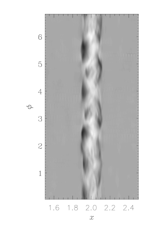
Figure 5: The density for model $\varepsilon=2$ during the unstable evolution, around $t_{A}=7.3$, along the plane $z=0$ as a function of radial and azimuthal coordinate. The presence of a higher $m$ mode around $m\sim 9$ is clearly visible. The domain along $\varphi$ is $2\pi$ and the resolution of the simulation along the $(z,r,\varphi)$ box is $240\times 120^{2}$.

Fig.(5) shows the occurrence of high $m$ modes for the density in the $(s,\varphi)$ plane for $\varepsilon=2$ for a $240\times 120^{2}$ simulation. It is difficult to reproduce the instability for much higher values of $\varepsilon$. As it is clear from Fig.(2) the width of the resonance is quite narrow in this case, the growth rate is significantly different from zero only for very large values of $m$ and the resolution in all three directions needed to reproduce the instability can be extremely large.

V Astrophysical implications and conclusions

In this paper, we revisited the stability properties of the screw pinch, a problem which has received considerable attention in the past in the context of MHD plasma stability for thermonuclear fusion. As it was pointed out by Freidberg frei70 , Eq.(2) describes various types of modes which can become unstable under certain conditions. The basic properties of the unstable modes are similar to those of quasi-kinks and quasi-interchanges obtained by goed71b ; goed72 for compressible plasma. However, astrophysical condition like those of stellar interior imply a high $\beta$ plasma parameter, a regime which is very far from the typical laboratory conditions. To the best of our knowledge, an instability of this type has not yet been extensively studied for a pressure balanced mixed poloidal/toroidal field configuration in the incompressible limit, an approximation which can be applied to various astrophysical situations. The following properties characterize the instability in this case: i) the instability does not occur for a current-free magnetic configuration; ii) it can arise on a time scale comparable to the Alfvén time scale whereas the growth rate calculated by goed72 is an order of magnitude lower, at least; iii) the eigenfunctions for high values of $m$ have a resonant character being very localized as shown in Fig.(4) for $m=6$; iv) the dependence of the growth rate on $m$ seems also to be rather peculiar. In the case of the instability described in goed72 , unfortunately, the growth rate is calculated only in the so called tokamak approximation $B_{\varphi}/xB_{z}\ll 1$ (see Eqs.(30)-(31) by goed72 ) and increases approximately proportional to $m$ or even faster. In our case, the dependence on $m$ is qualitatively different because the growth rate saturates with $m$ very rapidly, as noticed in the numerical investigation and in the approximate expression (7).

In spite of these differences, quasi-kink and quasi-interchange instabilities obtained by goed71b ; goed72 also have the typical double-peak structure depicted in Fig.(1) and Fig.(2) as a function of the the axial wavevector.

Note that the basic state in our model is characterized by the negative pressure gradient in some fraction of the volume, at least. Indeed, hydrostatic equilibrium with the toroidal field (10) implies that

$$\frac{dP}{ds}=-\frac{B_{\varphi}^{2}}{2\pi s}\left(1-\frac{s(s-s_{0})}{d^{2}}\right)$$ (11)

Then, $dP/ds<0$ if $d^{2}>s(s-s_{0})$. The condition $dP/ds<0$ is required for the development of instability (see, e.g., long ). The sign of the pressure gradient is important because it determines the destabilizing effect in the so called Suydam’s criterion suy . This criterion represents a necessary but local condition for stability and it reads in our notations

$$\frac{sB_{z}^{2}}{4\pi}\left(\frac{1}{h}\frac{dh}{ds}\right)^{2}+8\frac{dP}{ds}>0,$$ (12)

where $h=sB_{z}/B_{\varphi}$ is the magnetic shear. In the case of the basic state with toroidal field (10), the necessary condition for stability is not satisfied in some fraction of the volume (for example, in a neighborhood of $s_{0}$). This violation of the stability condition (12) is actually indicating the presence of at least some unstable mode in the system.

Stability properties of magnetic configurations are of great importance for various astrophysical applications. For instance, it is widely believed that magnetic fields play an important role in the formation and propagation of astrophysical jets providing an efficient mechanism of collimation through magnetic tension forces (e.g., blan ). Polarization observations provide information on the orientation and degree of order of the magnetic field in jets. It appears that many jets can develop relatively highly organized magnetic structures. To explain the observational data, various simplified models of three-dimensional magnetic structures have been proposed. Typically, the magnetic field can have both longitudinal component and substantial toroidal component in the core region (see, e.g., gab ). The mechanisms responsible for generation of the magnetic field in jets are still unclear. Since the origin of jets is probably relevant to MHD-processes in magnetized plasma, their magnetic fields could be generated during the process of jet formation (see, e.g., rom ) or, alternatively, it can be generated by the dynamo mechanism urp when the jet propagates in the interstellar medium. In both cases, the stability is a crucial issue for the properties of the jet. For instance, the origin of relatively small scale structures within the jet can be attributed to different instabilities arising in jets, including the one considered in our study. Magnetic structures that appears as a result of the development of instabilities can manifest themselves in polarization observations of the jets.

The considered instability can play an important role in magnetic stars where it can affect the magnetic field in stably stratified regions. Spruit spr reviewed various types of instabilities that are likely to intervene in a magnetized radiative regions of stars, and he concluded that the strongest among them are those which are related to the instability of magnetic configurations. According to spr , turbulence generated by such instability can drive a genuine dynamo in stellar radiative zones (see, however, zahn ). Understanding the conditions required for the instability is, therefore, crucial for dynamo models in stably stratified zones of stars.

This type of magnetic instabilities can be of interest also for neutron stars where the magnetic field reaches an extremely high value $\sim 10^{13}-10^{14}$ G. Such a strong field can be generated by the turbulent dynamo action during the very early stage of evolution (see bon ) when the neutron star is convectively unstable. This unstable stage lasts less than $\sim 1$ min. The further evolution of the magnetic field is determined mainly by ohmic dissipation but can be affected by current-driven instabilities as well land because dynamo in the convective zone generates a magnetic configuration that is not equilibrium.

Acknowledgments. VU thanks INAF-Ossevatorio Astrofisico di Catania for hospitality and financial support. All the computations were performed on the sanssouci-cluster of AIP whose support is gratefully acknowledged.

References

- (1)
- (2) Freidberg, J.P.: Ideal Magnetohydrodynamics. Plenum Press (1987);
- (3) Bernstein, I.B., Frieman, E.A., Kruskal, M.D., Kulsrud, R.M., Proc. R. Soc. A244, 17 (1958)
- (4) Wright G.A.E. Mon. Not. R. astr. Soc. 162, 339 (1973)
- (5) Tayler R.J. Mon. Not. R. astr. Soc. 161, 365 (1973)
- (6) Tayler R.J. Mon. Not. R. astr. Soc. 163, 77 (1973)
- (7) Tayler R.J. Mon. Not. R. astr. Soc. 191, 151 (1980)
- (8) Goedbloed, H., Poedts, S., Principles of Magnetohydrodynamics, CUP, (2004)
- (9) de Blank H.J., Transaction of Fusion science and Technology vol. 4 feb. 2006,
- (10) Bonanno A., Urpin V. Astron. Astrophys. 477, 35 (2008)
- (11) Bonanno A., Urpin V. Astron. Astrophys. 488, 1 (2008)
- (12) Braithwaite J., Spruit H. Nature 431, 819 (2004)
- (13) Braithwaite J., Nordlund A. Astron. Astrophys. 450, 1077 (2006)
- (14) Braithwaite J. Mon. Not. R. astr. Soc. 386, 1947 (2008)
- (15) Braithwaite J. Mon. Not. R. astr. Soc. 397, 763 (2009)
- (16) Duez, V.; Braithwaite, J.; Mathis, S., ApJ 724L, 24 (2010)
- (17) Bonanno A., Urpin V. Astron. Astrophys. 525, 100 (2011)
- (18) Freidberg J. Phys. Fluids. 13, 1812 (1970)
- (19) Goedbloed J.P. Physica. 53, 501 (1971)
- (20) W.H.Press, S.A.Teukolsky, W.T.Vetterling, and B.P.Flannery. Numerical Recipes in FORTRAN. The art of scientific computing (Cambridge UP, 1992).
- (21) Hayes, J. C., Norman, M. L., Fiedler, R. A., Bordner, J. O., Li, P. S., et al. ApJS, 165, 188 (2006)
- (22) Goedbloed J.P. Physica. 53. 535 (1971)
- (23) Goedbloed J.P., Hagebeuk H. Phys. Fluids. 15, 1090 (1972)
- (24) Longaretti P.-Y. 2003. PhLA, 320, 215
- (25) B.R. Suydam, in: Proc. of the Second U.N. Internat. Conf. on the Peaceful Uses of Atomic Energy, Vol. 31, United Nations, Geneva, 1958, p. 157.
- (26) Blandford R. 1993. In ”Astrophysical Jets” (Eds. D.Burgarella, M.Livio & C.P.O’Dea), Cambridge: Cambridge University Press Königl A., Pudritz R. 1999. In ”Protostars and Planets III” (Eds. V.Mannings, A.Boss & S.Russell), Tucson: University of Arizona Press
- (27) Hirabayashi H. et al. 1998. Science, 281, 1825; Gabuzda D., Murray E., Cronin P. 2004. MNRAS, 351, 89L
- (28) Blandford R., Payne D. 1982. MNRAS, 199, 883; Romanova M., Lovelace R. 1992. A&A, 262, 26; Koide S., Shibata K., Kudoh T. 1998. ApJ, 495, L63
- (29) Urpin V. 2006. A&A, 455, 779
- (30) Spruit H. 1999. A&A, 349, 189
- (31) Zahn J.-P., Brun A., Mathis S. 2007. A&A, 474, 145
- (32) Bonanno A., Rezzolla L., Urpin V. 2003, A&A, 410, 33; Bonanno A., Urpin V., Belvedere G. 2005. A&A, 440, 199; Bonanno A., Urpin V., Belvedere G. 2006. A&A, 451, 1049
- (33) Lander S.K., Jones D.I. 2011. MNRAS, 412, 1394; Kiuchi K., Yoshida S., Shibata M. 2011. astro-ph/1104.5561