On the collective curvature radiation

Abstract

The paper deals with the one possible mechanism of the pulsar radio emission, i.e., with the collective curvature radiation of the relativistic particle stream moving along the curved magnetospheric magnetic field lines. It is shown that the electromagnetic wave containing one cylindrical harmonic $\exp\{is\phi\}$ can not be radiated by the curvature radiation mechanism, that corresponds to radiation of a charged particle moving along curved magnetic field lines. The point is that the particle in vacuum radiates the triplex of harmonics ($s,s\pm 1$), so for the collective curvature radiation the wave polarization is very important and cannot be fixed a priori. For this reason the polarization of real unstable waves must be determined directly from the solution of wave equations for the media. Its electromagnetic properties should be described by the dielectric permittivity tensor ${\hat{\varepsilon}}(\omega,{\bf k,r})$, that contains the information on the reaction on all possible types of radiation.

1 Introduction

The curvature radiation is the type of the bremsstrahlung radiation when a radiated charged particle moves along the curved trajectory with the curvature radius $\rho_{0}$ and its acceleration is orthogonal to the velocity ${\bf v}$. The cyclotron rotation of a charged particle in the external magnetic field $B$ is the example of this motion when $\rho_{0}=v_{\perp}/\omega_{\rm c}$. Here $\omega_{\rm c}$ is the cyclotron frequency, $\omega_{\rm c}=eB/{m_{e}}c\gamma$, $e$ and $m_{\rm e}$ are the charge and the mass of a particle, $\gamma$ is the particle Lorentz factor, and $v_{\perp}$ is the component of the particle velocity which is orthogonal to the magnetic field.

Moving along the circular trajectory, a particle radiates at harmonics of the cyclotron frequency: $\omega=n\omega_{\rm c}$. This radiation is called as cyclotron radiation for a nonrelativistic particle and as synchrotron radiation for a relativistic particle ($\gamma\gg 1$). For the synchrotron radiation the maximum of the radiated power turns to be at large numbers of cyclotron harmonics: $n\simeq\gamma^{3}$. The total radiation power $I$ also grows with the particle energy, $I\propto\gamma^{2}$. Therefore, the synchrotron radiation of relativistic particles is presented widely in the space radiation (Ginzburg & Syrovatskii 1964).

It is necessary to stress that the length of formation of the curvature radiation, though is larger than the wave length $\lambda$, is much less than curvature radius $\rho_{0}$. So, the properties of the curvature radiation do not differ from that of the synchrotron radiation in which the cyclotron radius is equal to the local curvature radius $\rho_{0}$. The frequency of the maximum of the spectral power, $\omega\simeq c\gamma^{3}/\rho_{0}$, and radiation power, $I=4/3\,e^{2}c\gamma^{4}/\rho_{0}^{2}$, increases with the particle energy. Here the dependence on $\gamma$ is stronger than for the synchrotron radiation because the curvature is fixed, and does not fall with the energy as for the motion in the constant magnetic field.

The curvature mechanism of radiation is believed to be connected with the mechanism of the coherent pulsar radio emission. Indeed, in the region of the open magnetic field lines in the pulsar magnetosphere there is a relativistic electron-positron plasma moving with relativistic velocities along curved magnetic field lines. For the typical values of curvature radius, $\rho_{0}\simeq 10^{8}$ cm, and Lorentz factor of electrons and positrons, $\gamma\simeq 10^{2}$, the characteristic frequency of the curvature radiation is in the radio band. In the magnetosphere, where the curvature frequency coincides with the plasma frequency, $\omega_{\rm p}/\gamma^{3/2}$, we can expect the collective curvature radiation. Here $\omega_{\rm p}=(4\pi e^{2}n_{\rm e}/m_{\rm e})^{1/2}$ is the usual plasma frequency, and $n_{\rm e}$ is the plasma number density. In the strong magnetic field of the pulsar magnetosphere, when the charged particles can move along magnetic field lines only, the frequency of the plasma oscillations is $\gamma^{-3/2}$ times less than the usual plasma frequency $\omega_{\rm p}$.

It seems natural to continue the analogy between the curvature radiation and the cyclotron radiation for the collective radiation. But there is the essential difference between them, which does not permit to rewrite formulas of cyclotron plasma radiation for the curvature radiation replacing the cyclotron radius by the curvature radius. The matter is that at each point of plasma in the magnetic field the distribution of particles over transverse velocities is isotropic. All directions of particle transverse motion exist, so that the average velocity equals zero. It is not so for the curvature radiation when all particles have only one direction of motion along the magnetic field.

For the plasma physics the problem of the collective curvature radiation is rather complicated since it demands the consideration of an essentially nonuniform plasma. It does not result from the change of parameters of magnetic field and plasma in space. These effects can be taken into account in the local approximation because the wave length of radiation is much less than the scales of inhomogeneities. In order not to lose the curvature radiation we need to include into consideration the turn of the vector of anisotropy of the particle distribution function, $f({\bf p})\propto\delta({\bf p}-p_{\parallel}{\bf B}/B)$, in space. Here $p_{\parallel}$ is the longitudinal particle momentum.

Two parameters of the curvature radiation, i.e., the length of formation $l_{\rm f}=\rho_{0}/\gamma\simeq\lambda\gamma^{2}\gg\lambda$ and the width of the radiation directivity $\delta\phi\simeq\gamma^{-1}$, connect by the relation $l_{\rm f}/\rho_{0}\simeq\delta\phi$. Thus, the particle is in the synchronism with the wave (i.e., the particle sees the constant wave phase) along the path on which the wave intensity changes essentially. The value of $\lambda$ is the wave length of the curvature radiation, $\lambda\simeq\rho_{0}/\gamma^{3}$.

The problem of calculation of the dielectric permittivity in the geometrical optics approximation for the nonuniform anisotropic plasma particle distribution was solved by Beskin, Gurevich and Istomin (below BGI, 1993). They also described the collective curvature-plasma interaction, when the electromagnetic waves, connected with the curvature radiation, are amplified simultaneously by the Cherenkov mechanism. This effect is absent in the vacuum. However, this procedure is rather complicated and demands clear understanding. Because of that there are some incorrect statements in the literature (see, e.g., Nambu 1989; Machabeli 1991, 1995).

Apart, another way of investigation of the problem of the collective curvature radiation was carried out during many years (Asseo et al. 1983; Larroche & Pellat 1987; Lyutikov et al. 1999; Kaganovich & Lyubarsky 2010). They considered more simple task connected with the pure cylindrical geometry which can be solved ”exactly”. In such a statement the magnetic field lines are considered to be concentric, the relativistic plasma moving (i.e., rotating) along the magnetic field lines owing to the centrifugal drift directed parallel to the cylindrical axis ($z$-coordinate) with the velocity $u=c\rho_{c}/\rho_{0}\ll c$. Here again $\rho_{c}=c/\omega_{\rm c}$. But this approach cannot be used when analyse the curvature radiation (Beskin, Gurevich & Istomin 1988).

Indeed, let us choose the electromagnetic fields of the wave, as was done in all the papers mentioned above, in the form

$$\left({\bf E},{\bf B}\right)=\left({\bf E}(\rho),{\bf B}(\rho)\right)\times\exp\left\{-i\omega t+is\phi+ik_{z}z\right\}.$$ (1)

Here $\omega$ is the wave frequency, $s$ is integer number defining the azimuthal wave vector $k_{\phi}$, and $k_{z}$ is the longitudinal wave vector along the cylinder. In this approach the wave amplitudes ${\bf E}(\rho),{\bf B}(\rho)$ are to be considered as functions of the radial distance $\rho$ only. Moreover, not vectors ${\bf E}$ and ${\bf B}$, but their cylindrical components $(E,B)_{\rho},(E,B)_{\phi}$ and $(E,B)_{z}$ depend on the coordinate $\rho$ only. It means that the wave polarization follows the magnetic field, turning from one point $\phi$ to another. It can be so if we have the definite boundary condition, e.g., putting the system into the metallic coat. Under such suggestions we come to the one dimensional problem, which can be easily solved. Here we will show that such a wave does not have any relation to the curvature radiation.

Really, let us consider the particle moving exactly along the circle of radius $\rho_{0}$ with the constant velocity $v$; this motion corresponds to the infinite magnetic field. Then the radiated power is equal to the work of the wave electric field under the particle electric current. The electric current is

$${\bf j}=ev\delta(\phi-\Omega t)\,\delta(z)\frac{\delta(\rho-\rho_{0})}{\rho}\,{\bf e}_{\phi},$$ (2)

where $\Omega=v/\rho_{0}$, and for selected polarization we get

$$\int{\bf jE}{\rm d}{\bf r}=evE_{\phi}(\rho_{0})\exp\left\{-i\omega t+is\Omega t\right\}.$$ (3)

As we see, the radiation is possible only if $\omega-s\Omega=0$, i.e., $\omega=k_{\phi}v$. It is just the condition of Cherenkov, not curvature radiation. The point is that the wave with such polarization can not be radiated by the curvature mechanism. The difference between the curvature wave and the Cherenkov wave is in the finite interaction time of the bremsstrahlung radiation with a radiated particle. The freely propagating wave with almost constant polarization deflects from the direction of a particle motion. As a result, the nonzero projection of the wave electric field on the particle velocity (i.e., on the direction of the electric current) occurs, and the wave takes away the energy from the particle. This continues the finite time $\tau=l_{f}/v$ that can be determined from the relation $\tau(\omega-{\bf kv})\simeq 1$. For the relativistic particle ($v\simeq c$) $\tau=(\rho_{0}^{2}/\omega c^{2})^{1/3}\simeq\rho_{0}/c\gamma$. Below we will find the real polarization of the curvature radiation.

The paper is organized as follows. In section 2 we will find that the polarization of the curvature wave does not correspond to one cylindrical harmonic. In section 3 it is shown that the nonlinear wave interaction can lead to significant changes in cylindrical modes propagation. In section 4 the BGI permittivity tensor will be derived from the permittivity corresponding to one cylindrical mode. Finally, in section 5 we discuss the main results of our consideration.

2 Polarization of the curvature wave

The radiation field of the electric current density ${\bf j}$ and the electric charge density $\rho_{\rm e}$ of the moving particle with the charge $e$ is described by the retarded potentials (Landau & Lifshits 1975):

$${\bf A} = \frac{1}{c}\int\frac{{\bf j}(t^{\prime})}{R}{\rm d}{\bf r},$$ (4)

$$\Phi = \int\frac{\rho_{\rm e}(t^{\prime})}{R}{\rm d}{\bf r}.$$ (5)

Here $t^{\prime}=t-R/c$ is the retarded time, $R$ is the distance from the charge location at the time $t^{\prime}$ to the observer which has the cylindrical coordinates $(\rho,\phi,z)$,

$$R = \left[\rho^{2}+z^{2}+\rho_{0}^{2}-2\rho\rho_{0}\cos(\phi^{\prime}-\phi)\right]^{1/2},$$ (6)

$$\phi^{\prime} = \Omega t^{\prime}.$$ (7)

After the Fourier transformation of potentials (4)–(5) over the time we obtain

$${\bf A}_{\omega} = \frac{1}{2\pi}\int{\bf A}(t)\exp\{i\omega t\}{\rm d}t,$$ (8)

$$\Phi_{\omega} = \frac{1}{2\pi}\int\Phi(t)\exp\{i\omega t\}{\rm d}t.$$ (9)

It is convenient now to replace the integration over time $t$ by the integration over the retarded time $t^{\prime}$ and then over the angle $(\phi^{\prime}-\phi)$. As a result one can obtain for the cartesian components ($x,y,z$) of the vector potential ${\bf A}$ and the scalar potential $\Phi$

$$\left[{\bf A}_{\omega};\,\Phi_{\omega}\right]=\frac{e\rho_{0}}{2\pi c}\exp\{i\omega\phi/\Omega\}\left[-K_{s};\,K_{c};\,0;\,\frac{c}{v}K_{0}\right].$$ (10)

Here the quantities $K_{0},K_{s},K_{c}$ are the functions of coordinates $\rho$ and $z$ only and they are equal to

$$K_{0} = \int\frac{\exp\{i\omega(R/c+\Omega^{-1})\alpha\}}{R+v\rho\sin\alpha/c}{\rm d}\alpha,$$

$$K_{s} = \int\frac{\exp\{i\omega(R/c+\Omega^{-1})\alpha\}\sin\alpha}{R+v\rho\sin\alpha/c}{\rm d}\alpha,$$ (11)

$$K_{c} = \int\frac{\exp\{i\omega(R/c+\Omega^{-1})\alpha\}\cos\alpha}{R+v\rho\sin\alpha/c}{\rm d}\alpha,$$

$$R = (\rho^{2}+z^{2}+\rho_{0}^{2}-2\rho\rho_{0}\cos\alpha)^{1/2}.$$

The expression (10) is valid at any point ${\bf r}$, i.e., not only in the wave zone. The dependence over the angle $\phi$ is given by the exponent $\exp\{i\omega\phi/\Omega\}$. From the periodicity over $\phi$ we have $\omega=s\Omega$.

The key point of the above expansion (10) is that the radiated wave is the superposition of three harmonics: $s$,$s-1$, and $s+1$. For example, the azimuthal electric field $E_{\phi\omega}$ is equal to

$$E_{\phi\omega}=\frac{i\omega}{v}\left(-\frac{\rho_{0}}{\rho}\Phi_{\omega}+\frac{v}{c}A_{\phi\omega}\right)$$

$$=-i\frac{e\rho_{0}\omega}{2\pi v^{2}}e^{is\phi}\left[\frac{\rho_{0}}{\rho}K_{0}-\frac{v^{2}}{c^{2}}\left(K_{s}\sin\phi+K_{c}\cos\phi\right)\right].$$ (12)

The first term in Eqn. (12), which is proportional to the scalar potential $\Phi$, is not important in the wave zone, $\rho\gg\rho_{0}$, but is significant in the near zone on the particle trajectory $\rho=\rho_{0}$. Due to this term, the particle, which is in the resonance with one of three harmonics, say with $s$ ($\omega=s\Omega$), is beaten out of the synchronism by neighbour harmonics $s\pm 1$. The electric field $E_{\phi\omega}$ changes its sign during the time $\tau$. The synchronism condition, i.e., $1-\cos\Omega\tau\simeq 1-v^{2}/c^{2}=\gamma^{-2}$, defines the time $\tau$,

$$\tau\simeq 1/\Omega\gamma=\rho_{0}/c\gamma,$$ (13)

which coincides with the time of formation of the curvature radiation.

Thus, the radiated curvature wave consists of three harmonics $s,s\pm 1$ with the fixed relation between their amplitudes. Namely, this circumstance provides the curvature mechanism of the radiation. Appearance of harmonics $s\pm 1$ except the resonant one $s=\omega/\Omega$ is due to the additional modulation of the radiation field induced by a modulation of the particle electric current having the harmonic $s=1$. Now one can understand why the simple problem of the collective curvature radiation in the cylindrical geometry with only one azimuthal harmonic $\exp\{is\phi\}$ does not reveal any significant amplification of waves (Asseo et al., 1983; Lyutikov et al., 1999; Kaganovich & Lyubarsky, 2010). In this case the chosen wave polarization does not contain primordially the curvature mechanism.

3 Collective triple radiation

In the previous section it was shown that the curvature radiation of one charged particle can not be described in the pure cylindrical geometry by one azimuthal harmonic $\exp\{is\phi\}$. In a collective radiation the modulation of the particle electric current appears together with electromagnetic field excitation. Because of that the resonant azimuthal harmonic $s=\omega\rho/v_{\phi}$ mixes with harmonics of the electric current modulation and produces all possible values of $s$. Further in the section 4 we will see the all azimuthal harmonics $s$ give contribution to the response of a media on an electromagnetic field. But in this section it will be demonstrated that the collective curvature radiation of only triplex of azimuthal harmonics $(s,s\pm 1)$ differs significantly from that of one harmonic $s$ as it is usually considered in the literature.

Let us consider the simple cylindrical one-dimensional problem of radiation of the cold stream of plasma particles with the charge $e$ and the mass $m_{\rm e}$ moving along the infinite azimuthal magnetic field $B_{0}=B_{\phi}$. In this case the particles can move only in $\phi$-direction with the velocity $v_{\phi}$ at different cylindrical radius $\rho$. The unperturbed particle density $n^{(0)}$ and velocity $v_{\phi}^{(0)}$ are constants, i.e., they do not depend on $\rho$. The electric current ${\bf j}$ has only $\phi$-component as well as $B_{z}$-component of the wave magnetic field ($B_{\rho}=B_{\phi}=0$). Accordingly, the wave electric field has two components $E_{\rho}$ and $E_{\phi}$ ($E_{z}=0$).

The dependence of the wave fields over time and coordinates is the following

$$[E_{\rho};\,E_{\phi};\,B_{z}]=[E_{\rho}(\rho);\,E_{\phi}(\rho);\,B_{z}(\rho)]\exp\{-i\omega t+is\phi\}.$$ (14)

Then, we obtain from Maxwell equations

$$\frac{{\rm d}E^{(\sigma)}_{\phi}}{{\rm d}\rho}=\frac{i\sigma}{\rho}E^{(\sigma)}_{\rho}-i\frac{\rho}{\sigma}\frac{\omega^{2}}{c^{2}}E^{(\sigma)}_{\rho}-\frac{E^{(\sigma)}_{\phi}}{\rho},$$ (15)

$$\frac{{\rm d}E^{(\sigma)}_{\rho}}{{\rm d}\rho}=-i\frac{\sigma}{\rho}E^{(\sigma)}_{\phi}+\frac{4\pi}{\omega}\frac{\sigma}{\rho}j^{(\sigma)}_{\phi}-\frac{E^{(\sigma)}_{\rho}}{\rho}.$$ (16)

Here index $\sigma$ corresponds to one of three harmonics $s$ or $s\pm 1$. For simplicity we use here the dimensionless variable $r$ defined as $r=\rho\omega/c$, as well as quantities $\Lambda=\omega^{2}_{p}/(\omega^{2}\gamma^{3})$ and $J_{\sigma}=4\pi j^{(\sigma)}_{\phi}/(\Lambda\omega)$. Here $\omega_{\rm p}=(4\pi ne^{2}/m_{e})^{1/2}$ is plasma frequency, and $\gamma$ is the Lorentz-factor of the particle motion: $\gamma=(1-v_{\phi}^{2}/c^{2})^{-1/2}$. After these definitions the equations above take the following form

$$\frac{{\rm d}E^{(\sigma)}_{\phi}}{{\rm d}r} = \frac{i\sigma}{r}E^{(\sigma)}_{\rho}-i\frac{r}{\sigma}E^{(\sigma)}_{\rho}-\frac{E^{(\sigma)}_{\phi}}{r},$$ (17)

$$\frac{{\rm d}E^{(\sigma)}_{\rho}}{{\rm d}r} = -i\frac{\sigma}{r}E^{(\sigma)}_{\phi}+\Lambda\frac{\sigma}{r}J_{\sigma}-\frac{E^{(\sigma)}_{\rho}}{r}.$$ (18)

As was already stressed, we consider here the interaction of three waves $s,s\pm 1$. It is important that they are not independent and their interaction is realized by the static electric field $[E_{\rho}(\rho);\,E_{\phi}(\rho)]\exp\{i\phi\}$ having the first azimuthal harmonic $s=1$. This electrostatic field turns to be the result of nonlinear interactions of high frequency neighbour harmonics $s$ and $s\pm 1$. Equations for the mode $s=1$ under the same definitions are

$$\frac{{\rm d}E_{\phi}}{{\rm d}r} = \frac{i}{r}E_{\rho}-\frac{E_{\phi}}{r},$$ (19)

$$\frac{{\rm d}E_{\rho}}{{\rm d}r} = -i\frac{1}{r}E_{\phi}+\Lambda Z-\frac{E_{\rho}}{r}.$$ (20)

Here $Z=4\pi nec/(\Lambda\omega)$.

To determine the response of the stream on the electromagnetic fields of the wave one can use the continuity and Euler equations

$$\frac{\partial n}{\partial t}+{\rm\nabla}(n{{\bf v}})=0,$$ (21)

$$\left(\frac{\partial}{\partial t}+{\bf v}\nabla\right){\bf p}=e\left({\bf E}+\left[\frac{{\bf v}}{c},{\bf B}\right]\right).$$ (22)

It is easily to understand that only the $\phi$-component of Euler equation is needed, while the radial component just provides us the equilibrium configuration across the infinite magnetic field. We represent the plasma number density and the plasma velocity as the expansion over powers of the wave amplitude

$$v_{\phi}=v^{(0)}_{\phi}+\delta v^{(1)}_{\phi}+\delta v^{(2)}_{\phi}+...,$$ (23)

$$n=n^{(0)}+\delta n^{(1)}+\delta n^{(2)}+....$$ (24)

The linear response can be easy found

$$n^{(1)} = n^{(0)}\frac{kv^{(1)}_{\phi}}{\omega-kv_{\phi}^{(0)}},$$ (25)

$$v^{(1)}_{\phi} = i\frac{eE_{\phi}}{m_{\rm e}\gamma^{3}(\omega-kv_{\phi}^{(0)})},$$ (26)

where $k=s/\rho$. On the other hand, for the nonlinear current the nonlinear relation between $\delta v_{\phi}$ and $\delta p_{\phi}$ should be taken into account

$$\delta p_{\phi}=m_{\rm e}\gamma^{3}\delta v_{\phi}-\frac{3}{2}m_{\rm e}v^{(0)}_{\phi}\gamma^{5}\frac{(\delta v_{\phi})^{2}}{c^{2}}.$$ (27)

The result of cumbersome but straightforward calculation is

$$J_{s}=\frac{1}{1-sv^{(0)}_{\phi}/r}\left[i\frac{E^{s}_{\phi}}{1-sv^{(0)}_{\phi}/r}+\alpha\frac{r}{v^{(0)}_{\phi}}\left(A_{s,s-1}\frac{E^{s-1}_{\phi}E^{1}_{\phi}}{1-(s-1)v^{(0)}_{\phi}/r}-A_{s,s+1}\frac{E^{s+1}_{\phi}E^{1*}_{\phi}}{1-(s+1)v^{(0)}_{\phi}/r}\right)\right],$$ (28)

$$J_{s-1}=\frac{1}{1-(s-1)v^{(0)}_{\phi}/r}\left[i\frac{E^{s-1}_{\phi}}{1-(s-1)v^{(0)}_{\phi}/r}-\alpha\frac{r}{v^{(0)}_{\phi}}A_{s,s-1}\frac{E^{s}_{\phi}E^{1*}_{\phi}}{1-sv^{(0)}_{\phi}/r}\right],$$ (29)

$$J_{s+1}=\frac{1}{1-(s+1)v^{(0)}_{\phi}/r}\left[i\frac{E^{s}_{\phi}}{1-(s+1)v^{(0)}_{\phi}/r}+\alpha\frac{r}{v^{(0)}_{\phi}}A_{s,s+1}\frac{E^{s}_{\phi}E^{1}_{\phi}}{1-sv^{(0)}_{\phi}/r}\right],$$ (30)

$$Z=\frac{1}{\left(v^{(0)}_{\phi}\right)^{2}}\left[i\frac{E_{1}}{1/r}+\alpha\left(\frac{E^{s+1}_{\phi}E^{s*}_{\phi}}{(1-(s+1)v^{(0)}_{\phi}/r)(1-sv^{(0)}_{\phi}/r)}+\frac{E^{s}_{\phi}E^{(s-1)*}_{\phi}}{(1-sv^{(0)}_{\phi}/r)(1-(s-1)v^{(0)}_{\phi}/r)}\right)\right],$$ (31)

$$A_{i,j}=\frac{1}{1-iv^{(0)}_{\phi}/r}+\frac{1}{1-jv^{(0)}_{\phi}/r}-3\gamma^{2},$$

Here $\alpha=e/(m_{e}c\gamma^{3}\omega)$ is the particle velocity divided over the velocity of light. The same quantities for plane waves can be found in (BGI, 1993). Equations above are evaluated with vacuum initial condition for the normal mode that can be presented analytically, $E^{(\sigma)}_{\phi}=-J^{{}^{\prime}}_{\sigma}(r),E^{(\sigma)}_{r}=i{\sigma}J_{\sigma}(r)/r$. Here $J_{\sigma}(r)$ is the Bessel function. It should be noted that the singularity in equations (17) is passed smoothly by additional small term $+i\varepsilon$ in the resonance denominators in (25)–(26).

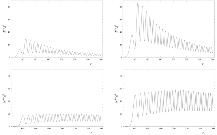
Figure 1: Model calculations of two cases, $\Lambda=10^{-2}$, $\nu=1GHz$, $\gamma=5$, $s=125$.

In numerical calculations equations (17)–(20) for $\sigma=s$ and $\sigma=s\pm 1$ were solved with two different values for the quantities $J_{\sigma}$ and $Z$. In the first case we neglect non-linear terms in (28)–(31), while the second one corresponds to the full non-linear problem. On Fig.  1 the results obtained for this cases are presented. For better representation of the influence of the nonlinear current, we choose the amplitudes of $s-1$ and $s+1$ modes twenty times higher than the amplitude of the $s$ mode. In reality the $s$-mode interacts with the whole continuum of modes, so this model assumption is rather reasonable. Fig.  1 shows that in this case the intensity of the wave $|E|^{2}$ is approximate 2.5 times larger than in the case when the nonlinear current is neglected. Hence, one can conclude that three wave interaction is rather effective.

Thus, we have shown that the triplex of cylindrical harmonics, which corresponds better to the curvature mechanism, is amplified more effective than the separated harmonic having the single value of the azimuthal number. In fact the real polarization of the collective curvature mode can be obtained only by calculating the permittivity tensor of the streaming plasma in the strong curved magnetic field. The solution of wave equations produces not only the dispersive equation for normal waves, $\omega=\omega({\bf k})$, but defines also their polarization. A priory it is unclear what polarization corresponds to unstable modes.

At first sight, the problem considered above is essentially nonlinear and has no direct connection with the question of the linear wave amplification. We included nonlinearity only in order to connect harmonics $s,\,s\pm 1$ self-consistently. And appearance of neighbour harmonics $s\pm 1$, even for small nonlinearity, strongly change the $s$-mode amplification. It is clear also that interaction of $s\pm 1$ waves with the field $s=1$ will result in all azimuthal harmonics.

4 Tensor derivation

In this section we will show that the asymptotic behaviour of the BGI dielectric tensor in the case of large enough curvature radius $\rho_{0}$ can be found directly from the plasma response on the one cylindrical mode. For the infinite toroidal magnetic field only the response to the toroidal component of the wave electric field $E_{\phi}$ is to be included into consideration (Beskin 1999). Here and below we consider the stationary medium only, so the time dependence can be chosen as $\exp\{-i\omega t\}$. Making summation over all cylindrical modes, one can write down

$$D_{\phi}(\rho,\phi)=E_{\phi}(\rho,\phi)-\sum\limits_{s=-\infty}^{\infty}E_{\phi}(\rho,s)K(\rho,s)\exp\{is\phi\},$$ (32)

where

$$K(\rho,s)=\frac{4\pi e^{2}}{\omega}\int\frac{v_{\phi}}{\omega-sv_{\phi}/\rho}\frac{\partial f^{(0)}}{\partial p_{\phi}}{\rm d}p_{\phi}.$$ (33)

Here $f^{(0)}(p_{\phi})$ is unperturbed distribution function. Making the Fourier transformation

$$E_{\phi}(\rho,s)=\frac{1}{2\pi}\int\limits_{0}^{2\pi}E_{\phi}(\rho,\phi^{\prime})\exp\{-is\phi^{\prime}\}{\rm d}\phi^{\prime}$$ (34)

and the transition to cartesian coordinate system one can obtain:

$$D_{x}=E_{x}+\frac{1}{2\pi}\int\frac{\rho^{\prime}{\rm d}\rho^{\prime}{\rm d}\phi^{\prime}}{\rho^{\prime}}\sum\limits_{s=-\infty}^{\infty}E_{\phi}(\rho^{\prime},\phi^{\prime})\delta(\rho-\rho^{\prime})\times$$

$$K(\rho,s)\,\exp\{is(\phi-\phi^{\prime})\}\sin\phi,$$ (35)

$$D_{y}=E_{y}-\frac{1}{2\pi}\int\frac{\rho^{\prime}{\rm d}\rho^{\prime}{\rm d}\phi^{\prime}}{\rho^{\prime}}\sum\limits_{s=-\infty}^{\infty}E_{\phi}(\rho^{\prime},\phi^{\prime})\delta(\rho-\rho^{\prime})\times$$

$$K(\rho,s)\,\exp\{is(\phi-\phi^{\prime})\}\cos\phi.$$ (36)

We choose the local coordinate system with the $y$-axis directed along the magnetic field and the $x$-axis, that is orthogonal to it. From the above equations one can obtain the permittivity kernel components

$$\varepsilon_{yy}({\bf{r}},{\bf{r^{\prime}}})=1-\frac{1}{2\pi}\frac{1}{\rho^{\prime}}\sum\limits_{s=-\infty}^{\infty}\delta(\rho-\rho^{\prime})K(\rho,s)\times$$

$$\exp\{is(\phi-\phi^{\prime})\}\cos\phi\cos\phi^{\prime};$$ (37)

$$\varepsilon_{yx}({\bf{r}},{\bf{r^{\prime}}})=\frac{1}{2\pi}\frac{1}{\rho^{\prime}}\sum\limits_{s=-\infty}^{\infty}\delta(\rho-\rho^{\prime})K(\rho,s)\times$$

$$\exp\{is(\phi-\phi^{\prime})\}\cos\phi\sin\phi^{\prime};$$ (38)

$$\varepsilon_{xy}({\bf{r}},{\bf{r^{\prime}}})=\frac{1}{2\pi}\frac{1}{\rho^{\prime}}\sum\limits_{s=-\infty}^{\infty}\delta(\rho-\rho^{\prime})K(\rho,s)\times$$

$$\exp\{is(\phi-\phi^{\prime})\}\sin\phi\cos\phi^{\prime},$$ (39)

$$\varepsilon_{xx}({\bf{r}},{\bf{r^{\prime}}})=1-\frac{1}{2\pi}\frac{1}{\rho^{\prime}}\sum\limits_{s=-\infty}^{\infty}\delta(\rho-\rho^{\prime})K(\rho,s)\times$$

$$\exp\{is(\phi-\phi^{\prime})\}\sin\phi\sin\phi^{\prime},$$ (40)

that provides the material relationship

$$D_{i}({\bf{r}})=\int\varepsilon_{ij}({\bf{r}},{\bf{r^{\prime}}})E_{j}({\bf{r^{\prime}}}){\rm d}{\bf{r^{\prime}}}.$$ (41)

It should be noted that the operator presented above satisfies the needed symmetry condition

$$\varepsilon_{ij}({\bf{r}},{\bf{r^{\prime}}},\omega)=\varepsilon_{ji}({\bf{r^{\prime}}},{\bf{r}},-\omega)$$ (42)

(it is provided by the condition $K(r,s,\omega)=K(r,-s,-\omega)$). As it is well-known (Kadomtsev 1965; Bornatici & Kravtsov 2000), it is this symmetrical form of permittivity tensor that is to be used for the calculation of components of the permittivity tensor $\varepsilon_{ij}(\omega,{\bf{k}},{\bf{r}})$

$$\varepsilon_{ij}(\omega,{\bf{k}},{\bf{\boldsymbol{\eta}}}\to{\bf{r}})=\int\varepsilon_{ij}(\omega,{\bf{\boldsymbol{\xi}}},{\bf{\boldsymbol{\eta}}})\exp\{-i\bf{k\boldsymbol{\xi}}\}{\rm d}{\bf{r}}.$$ (43)

Here ${\boldsymbol{\boldsymbol{\eta}}}=({\bf r}+{\bf r^{\prime}})/2$, ${\bf\boldsymbol{\xi}}=\bf{r}-\bf{r^{\prime}}$. It is important that the above tensor only describes correctly wave-particle interaction in inhomogeneous media with slowly varying parameters (Bernstein & Friedland 1984).

Substituting now the kernel components, one can find

$$\varepsilon_{xx}(\omega,{\bf{k}},{\bf{\boldsymbol{\eta}}})=1-\frac{1}{2\pi}\int{\rm d}{\bf\boldsymbol{\xi}}\exp\{-i{\bf{k\boldsymbol{\xi}}\}}\frac{1}{|{\bf\boldsymbol{\eta}-\boldsymbol{\xi}}/2|}\times$$

$$\sum\limits_{s=-\infty}^{\infty}\delta(|{\bf\boldsymbol{\eta}+\boldsymbol{\xi}}/2|-|{\bf\boldsymbol{\eta}-\boldsymbol{\xi}}/2|)K(|{\bf\boldsymbol{\eta}+\boldsymbol{\xi}}/2|,s)\times$$

$$\exp\{is(\phi-\phi^{\prime})\}\sin\phi\sin\phi^{\prime},$$ (44)

$$\varepsilon_{xy}(\omega,{\bf{k}},{\bf{\boldsymbol{\eta}}})=\frac{1}{2\pi}\int{\rm d}{\bf\boldsymbol{\xi}}\exp\{-i{\bf{k\boldsymbol{\xi}}\}}\frac{1}{|{\bf\boldsymbol{\eta}-\boldsymbol{\xi}}/2|}\times$$

$$\sum\limits_{s=-\infty}^{\infty}\delta(|{\bf\boldsymbol{\eta}+\boldsymbol{\xi}}/2|-|{\bf\boldsymbol{\eta}-\boldsymbol{\xi}}/2|)K(|{\bf\boldsymbol{\eta}+\boldsymbol{\xi}}/2|,s)\times$$

$$\exp\{is(\phi-\phi^{\prime})\}\sin\phi\cos\phi^{\prime},$$ (45)

$$\varepsilon_{yx}(\omega,{\bf{k}},{\bf{\boldsymbol{\eta}}})=\frac{1}{2\pi}\int{\rm d}{\bf\boldsymbol{\xi}}\exp\{-i{\bf{k\boldsymbol{\xi}}\}}\frac{1}{|{\bf\boldsymbol{\eta}-\boldsymbol{\xi}}/2|}\times$$

$$\sum\limits_{s=-\infty}^{\infty}\delta(|{\bf\boldsymbol{\eta}+\boldsymbol{\xi}}/2|-|{\bf\boldsymbol{\eta}-\boldsymbol{\xi}}/2|)K(|{\bf\boldsymbol{\eta}+\boldsymbol{\xi}}/2|,s)\times$$

$$\exp\{is(\phi-\phi^{\prime})\}\cos\phi\sin\phi^{\prime},$$ (46)

$$\varepsilon_{yy}(\omega,{\bf{k}},{\bf{\boldsymbol{\eta}}})=1-\frac{1}{2\pi}\int{\rm d}{\bf\boldsymbol{\xi}}\exp\{-i{\bf{k\boldsymbol{\xi}}\}}\frac{1}{|{\bf\boldsymbol{\eta}-\boldsymbol{\xi}}/2|}\times$$

$$\sum\limits_{s=-\infty}^{\infty}\delta(|{\bf\boldsymbol{\eta}+\boldsymbol{\xi}}/2|-|{\bf\boldsymbol{\eta}-\boldsymbol{\xi}}/2|)K(|{\bf\boldsymbol{\eta}+\boldsymbol{\xi}}/2|,s)\times$$

$$\exp\{is(\phi-\phi^{\prime})\}\cos\phi\cos\phi^{\prime}.$$ (47)

In this equations, the angles $\phi$ and $\phi^{\prime}$ are the functions of polar angles of vectors $\bf{\boldsymbol{\eta}}$ and $\bf{\boldsymbol{\xi}}$, $\alpha_{\eta}$, and $\alpha_{\xi}$

$$\sin\phi=\frac{|\boldsymbol{\eta}|\sin\alpha_{\eta}+(|\boldsymbol{\xi}|/2)\sin\alpha_{\xi}}{|{\bf\boldsymbol{\eta}+\boldsymbol{\xi}}/2|},$$ (48)

$$\cos\phi^{\prime}=\frac{|\boldsymbol{\eta}|\cos\alpha_{\eta}-(|\boldsymbol{\xi}|/2)\cos\alpha_{\xi}}{|{\bf\boldsymbol{\eta}-\boldsymbol{\xi}}/2|}.$$ (49)

As a result, integrals above are reduced to integration over $\bf{\boldsymbol{\xi}}$, which is perpendicular to $\bf{\boldsymbol{\eta}}$. On the other hand, the expression for the delta-functions in (44)–(47) is the following:

$$\delta(...) = \frac{\delta(\theta-\pi/2)}{(|{\bf\boldsymbol{\eta}+\boldsymbol{\xi}}/2|-|{\bf\boldsymbol{\eta}-\boldsymbol{\xi}}/2|)^{\prime}_{\theta}}$$ (50)

$$+ \frac{\delta(\theta+\pi/2)}{(|{\bf\boldsymbol{\eta}+\boldsymbol{\xi}}/2|-|{\bf\boldsymbol{\eta}-\boldsymbol{\xi}}/2|)^{\prime}_{\theta}},$$

where $\theta$ is the angle between vectors $\bf{\boldsymbol{\eta}}$ and ${\bf{\boldsymbol{\xi}}}$. So, the integration over angles can be done easily. Finally, from the transition ${\bf{\boldsymbol{\eta}}}\to{\bf{r}}$, one can obtain $\cos\alpha_{\eta}\to\cos\alpha_{r}=1$. Hence, according to (50) $({\bf k\boldsymbol{\xi}})=k_{\parallel}|\boldsymbol{\xi}|$, where $k_{\parallel}$ is the component of the wave vector parallel to external magnetic field.

The property of the absence of $k_{\perp}$ is very important, it provides the same symmetry as it was in the case of homogeneous medium: $\varepsilon_{ij}(-\omega,-{\bf k},-{\bf B},{\bf r})=\varepsilon_{ji}(\omega,{\bf k},{\bf B},{\bf r})$ (Istomin 1994). This result differs from one obtained by Lyutikov at al. (1999). In this work the importance of transformation (43) is neglected.

Using finally the Taylor expansion over $|\boldsymbol{\xi}|$ and the reduction of resonant denominator to delta-function, one can obtain:

$$\sum(...)\frac{1}{\omega|{\bf\boldsymbol{\eta}+\boldsymbol{\xi}}/2|/v_{\phi}-s}$$

$$\to i\pi\int(...)\delta\left[s-\frac{\omega(|\boldsymbol{\eta}|^{2}+|\boldsymbol{\xi}|^{2}/4)^{1/2}}{v_{\phi}}\right]{\rm d}s.$$ (51)

As a result, one can write down

$$\varepsilon_{xx} = -i\frac{8\pi^{2}e^{2}}{\omega}\int F^{\prime\prime}(\kappa)\frac{v_{\phi}}{\omega}\frac{\partial f^{(0)}}{\partial p_{\phi}}{\rm d}p_{\phi},$$ (52)

$$\varepsilon_{xy} = -\varepsilon_{yx}=\frac{8\pi^{2}e^{2}}{\omega}\int F^{\prime}(\kappa)\frac{\rho^{1/3}_{0}v^{2/3}_{\phi}}{\omega^{2/3}}\frac{\partial f^{(0)}}{\partial p_{\phi}}{\rm d}p_{\phi},$$ (53)

$$\varepsilon_{yy} = -i\frac{8\pi^{2}e^{2}}{\omega}\int F(\kappa)\frac{\rho^{2/3}_{0}v^{1/3}_{\phi}}{\omega^{1/3}}\frac{\partial f^{(0)}}{\partial p_{\phi}}{\rm d}p_{\phi}.$$ (54)

Here

$$F(\kappa) = \frac{1}{\pi}\int\limits^{+\infty}_{0}\exp\{i\kappa t+it^{3}/3\}{\rm d}t,$$ (55)

$$\kappa = \frac{2(\omega-k_{\parallel}v_{\phi})}{\omega^{1/3}v^{2/3}_{\phi}}\rho^{2/3}_{0},$$ (56)

prime means the derivative, and $\rho_{0}$ is the curvature radius of magnetic field.

Due to high enough curvature radius of field lines in the pulsar magnetosphere, one can use the asymptotic behaviour of $F(\kappa)$ for $\kappa\gg 1$

$$F(\kappa)\approx\frac{i}{\pi\kappa}+\frac{2i}{\pi\kappa^{4}}+...$$ (57)

After integration by parts, the final result is

$$\varepsilon_{ij}=\begin{pmatrix}1-\frac{3}{2}\left<\frac{\omega^{2}_{pl}v^{2}_{\parallel}}{\gamma^{3}\rho^{2}_{0}\tilde{\omega}^{4}}\right>&&-i\left<\frac{\omega^{2}_{pl}v_{\parallel}}{\gamma^{3}\rho_{0}\tilde{\omega}^{3}}\right>\cr i\left<\frac{\omega^{2}_{pl}v_{\parallel}}{\gamma^{3}\rho_{0}\tilde{\omega}^{3}}\right>&&1-\left<\frac{\omega^{2}_{pl}}{\gamma^{3}\tilde{\omega}^{2}}\right>\cr\end{pmatrix}$$ (58)

Here by definition $\tilde{\omega}=\omega-{\bf kv}$, and the brackets $<>$ denote both the averaging over the particle distribution function $f_{e^{+},e^{-}}(p_{\phi})$ and the summation over the types of particles:

$$<(...)>\,=\sum_{e^{+}e^{-}}\int(...)f^{(0)}_{e^{+},e^{-}}(p_{\phi}){\rm d}p_{\phi}.$$ (59)

We see that the tensor above is just the BGI tensor, that leads to instability of the so-called curvature plasma modes. In the limit $\rho_{0}=\infty$ this tensor, as expected, tends to the dielectric permittivity of a homogeneous plasma. The nonzero components $\varepsilon_{xy},\varepsilon_{yx}$ and $\delta\varepsilon_{xx}=\varepsilon_{xx}-1$ in the tensor $\varepsilon_{ij}$ (58) for the finite curvature are due to nonlocal properties of the plasma response on the electromagnetic wave in curved magnetic field. The parameter of nonlocality $(v_{\parallel}/\tilde{\omega})/\rho_{0}$ is the ratio of the formation length of radiation to the curvature radius. For vacuum $\tilde{\omega}\simeq\omega/\gamma^{2}$, and the length $v_{\parallel}/\tilde{\omega}$ coincides with the length of formation of the curvature radiation $l_{f}$.

It is important that the components $\varepsilon_{xy}=-\varepsilon_{yx}$ and $\delta\varepsilon_{xx}$ essentially change the wave polarization. The relation between $E_{\phi}$ and $E_{\rho}$ of the wave electric field, following from the tensor of the dielectric permittivity (58), is

$$\left(\varepsilon_{xy}+n_{\rho}n_{\phi}\right)E_{\phi}+\left(\delta\varepsilon_{xx}+1-n_{\phi}^{2}\right)E_{\rho}=0,$$ (60)

where $n_{\rho}$ and $n_{\phi}$ are components of the dimensionless wave vector: ${\bf n}={\bf k}c/\omega$. For the tangent wave propagation (i.e., for $n_{\rho}=0$) we have $E_{\phi}\simeq(\delta\varepsilon_{xx}/\varepsilon_{xy})E_{\rho}\simeq(c/\rho_{c}\tilde{\omega})E_{\rho}$. As a result, a wave can produce the negative work under the electric particle current $j_{\phi}$, i.e., it can be excited. It is not so if $\delta\varepsilon_{xx}=\varepsilon_{xy}=0$ when $E_{\phi}=0$.

5 Discussion

Thus, as it was shown above, the wave polarization $[E_{\rho}(\rho);\,E_{\phi}(\rho)]\exp\{is\phi\}$ containing one cylindrical harmonic $s$ suggests only the Cherenkov mechanism of radiation. In the curvature radiation mechanism of one particle in vacuum the generated wave consists of three harmonics $s,s\pm 1$. This property provides the exit from the phase synchronism of the wave with the particle motion which is inherent in the bremsstrahlung radiation. For the collective curvature radiation it is shown that the hydrodynamical model of plasma motion along the infinite magnetic field gives different results of the wave amplification depending on the wave polarization. So, there is no another way to find the polarization of exiting waves instead of calculation of the response of the medium on an electromagnetic field, i.e., to use the dielectric permittivity. The correct procedure of dielectric permittivity calculation using the expansion over cylindrical modes is also shown above. It was demonstrated that the tensor obtained by this procedure coincides with the BGI tensor calculated previously by another method.

In conclusion it is worth to note that unsuccessful attempts to find the collective curvature radiation bring to the term ’curvature-drift instability’ (Lyutikov et al. 1999). As was shown the chosen simple wave polarization, i.e., one $s$-harmonic, means only the existence of the Cherenkov mechanism of the wave generation. In this case the centrifugal particle drift places the significant role. Practically all curvature effects come only to this drift. And the Cherenkov resonance on the drift motion produces small wave amplification in better case (Kaganovich & Lyubarsky 2010). Stronger magnetic field produces less drift velocity and less Cherenkov effect though the curvature of a particle motion does not depend on the magnetic field strength at all.

6 Acknowledgments

We thank A.V. Gurevich for his interest and support. This work was partially supported by Russian Foundation for Basic Research (Grant no. 11-02-01021).

References

• APS (1983) Asseo E., Pellat R., Sol H., 1983, Astrophys. J., 266, 201
• BK (2000) Bornatici M., Kravtsov Yu.A., 2000, Plasma Phys. Control Fusion, 42, 255
• Bernstein&Fried (1984) Bernstein I.B., Friedland L., 1984, Handbook of Plasma Physics vol. 1, ed. Galeev A. & Sudan R.N., North - Holland, Amsterdam
• Beskin & Gurevich & Istomin (1988) Beskin V.S., Gurevich A.V., Istomin Y.N., 1988, Phys. Rev. Let. 61, 649
• Beskin & Gurevich & Istomin (1993) Beskin V.S., Gurevich A.V., Istomin Y.N., 1993, Physics of the Pulsar Magnetosphere, Cambridge University Press, Cambridge
• Beskin (1999) Beskin V.S., 1999, Physics-Uspekhi, 169, 1169
• GS (1964) Ginzburg V.L., Syrovatskii S.I., 1964, The Origin of cosmic rays, Pergamon press, New York
• Istomin (1994) Istomin Ya.N., 1994, Plasma Phys. Control Fusion, 36, 1081
• Kadomtsev (1965) Kadomtsev B.B., 1965, Plasma Turbulence, Academic, New York
• LK (2010) Kaganovich A., Lyubarsky Y., 2010, Astrophys. J., 721, 1164
• Landau & Lifshits (1975) Landau L.D., Lifshits E.M., 1975, The Classical Theory of Fields, Pergamon Press
• Larroche (1987) Larroch O., Pellat R., 1987, Phys Rev. Lett., 59, 1104
• Larroche (1987) Lyutikov M., Machabeli G.Z., Blandford R., 1999, Astrophys. J., 512, 804
• M1 (1991) Machabeli G.Z., 1991, Plasma Phys. Control Fusion, 33, 1227
• M2 (1995) Machabeli G.Z., 1995, Plasma Phys. Control Fusion, 37, 177
• Nambu (1989) Nambu M., 1989, Plasma Phys. Control Fusion, 31, 143