Adiabatic quantum pumping through surface states in 3D topological insulators

Abstract

We investigate adiabatic quantum pumping of Dirac fermions on the surface of a strong 3D topological insulator. Two different geometries are studied in detail, a normal metal – ferromagnetic – normal metal (NFN) junction and a ferromagnetic – normal metal – ferromagnetic (FNF) junction. Using a scattering matrix approach, we first calculate the tunneling conductance and then the adiabatically pumped current using different pumping mechanisms for both types of junctions. We explain the oscillatory behavior of the conductance by studying the condition for resonant transmission in the junctions and find that each time a new resonant mode appears in the transport window, the pumped current diverges. We also predict an experimentally distinguishable difference between the pumped current and the rectified current.

I Introduction

Recently, surface states in topological insulators have attracted a lot of attention in the condensed-matter community Hasan2010 . Both in two-dimensional (e.g., HgTe) and in three-dimensional (e.g., Bi₂Se₃) compounds with strong spin-orbit interaction the topological phase has been demonstrated experimentally Konig2007 ; Hsieh2008 ; Xia2009a ; Xia2009b . Although these compounds are insulating in the bulk (since they have an energy gap between the conduction band and the valance band), their surface states support topological gapless excitations. In the simplest case these low-energy excitations of a strong three-dimensional topological insulator can be described by a single Dirac cone at the center of the two-dimensional Brillouin zone ($\Gamma$ point) Konig2007 ; Xia2009a ; Hsieh2009a ; Roushan2009 ; Hsieh2009b ; *HZhang2009. The corresponding Hamiltonian is given by Fu2008

$$\mathcal{H}_{0}=\hbar v_{F}\vec{\sigma}\cdot\vec{k}-\mu I.$$ (1)

Here $\vec{\sigma}$ represents a vector whose three components are the three Pauli spin matrices, $I$ represents a $2\times 2$ identity matrix in spin space, $v_{F}$ is the Fermi velocity, and $\mu$ is the chemical potential. The low-energy excitations of $\mathcal{H}_{0}$ [Eq. (1)] are topologically protected against perturbations TZhang2009 . This has prompted recent research on the transport properties of surface Dirac fermions. For example, the conductance and magnetotransport of Dirac fermions have been studied in normal metal – ferromagnet (NF), normal metal – ferromagnetic – normal metal (NFN) and arrays of NF junctions on the surface of a topological insulator Mondal2010a ; Mondal2010b ; Zhang2010 , suggesting the possibility of an engineered magnetic switch. An anomalous magnetoresistance effect has been predicted in ferromagnetic-ferromagnetic junctions Yokoyama2010 . Also, electron tunneling and magnetoresistance have been studied in ferromagnetic – normal metal – ferromagnetic (FNF) junctions Wu2010 ; Salehi2011 , for which it has been predicted that the conductance can be larger in the anti-parallel configuration of the magnetizations of the two ferromagnetic regions than in the parallel configuration. In addition, a large research effort has been devoted to studying models which predict the existence of Majorana fermion edge states at the interface between superconductors and ferromagnets deposited on a topological insulator Fu2008 ; Akhmerov2009 ; Tanaka2009 .

In this article we investigate adiabatic quantum pumping of Dirac fermions through edge states on the surface of a strong three-dimensional topological insulator. Quantum pumping refers to a transport mechanism in meso- and nanoscale devices by which a finite dc current is generated in the absence of an applied bias by periodic modulations of at least two system parameters (typically gate voltages or magnetic fields) Buttiker1994 ; Brouwer1998 ; Spivak1995 . In order for electrical transport to be adiabatic, the period of the oscillatory driving signals has to be much longer than the dwell time $\tau_{\rm dwell}$ of the electrons in the system, $T=2\pi\omega^{-1}\gg\tau_{\rm dwell}$. In the last decade, many different aspects of quantum pumping have been theoretically investigated in a diverse range of nanodevices, for example charge and spin pumping in quantum dots Switkes1999 ; Mucciolo2002 ; Sharma2003 ; Watson2003 , the role of electron-electron interactions Splettstoesser2005 ; Sela2006 ; Reckermann2010 , quantum pumping in graphene mono- and bilayers Prada2009 ; Zhu2009 ; Prada2010 ; Wakker2010 ; Tiwari2010 ; AlosPalop2011 ; Kundu2011 as well as charge and spin pumping through edge states in quantum Hall systems miriam2003 and recently a two-dimensional topological insulator Citro2011 . On the experimental side, Giazotto et al. Giazotto2011 have recently reported an experimental demonstration of charge pumping in an InAs nanowire embedded in a superconducting quantum interference device (SQUID).

Our main focus is to study quantum pumping induced by periodic modulations of gate voltages or exchange fields, which are induced by a ferromagnetic strip in two topological insulator devices: a NFN and a FNF junction, see Figs. 1 and 2. Using a scattering matrix approach, we obtain analytical expressions for the angle-dependent pumped current in both types of junctions. We find that the adiabatically pumped current in a NFN topological insulator junction induced by periodic modulations of gate voltages reaches maximum values at specific energy values. In order to explain the position of these values, we study in detail the conductance of the junctions. In particular, we provide an explanation for resonances in the conductance that were predicted but not explained in detail in the previous works Mondal2010a ; Mondal2010b . We show that each time a new resonant mode appears in the junction the conductance increases and the pumped current reaches a maximum value. For the FNF pump we predict a non-zero current by periodic modulation of the exchange magnetic coupling in the absence of external voltages. We observe and analyze basic similarities and differences between the two pumps studied in this paper and highlight an experimentally distinguishable feature between the pumped current and the conductance.

The remainder of the paper is organized as follows. In Sec. II, we describe the NFN and FNF junctions and use a scattering matrix model to calculate the reflection and transmission coefficients of both junctions. In Sec. III, we review the conductance of the NFN junction and present a detailed analysis of the plateau-like steps that appear in the conductance. We also analyze and compare the conductance of the FNF junction with parallel and anti-parallel configuration of the magnetization. In Sec. IV, we calculate the adiabatically pumped current for the two different pumps and derive analytical expressions as a function of the angle of incidence of the carriers. We also investigate the dependence of the pumped current and the conductance on the width $d$ of the middle region. Finally, in Sec. V we summarize our main results and propose possibilities for experimental observation of our predictions.

II NFN and FNF junctions

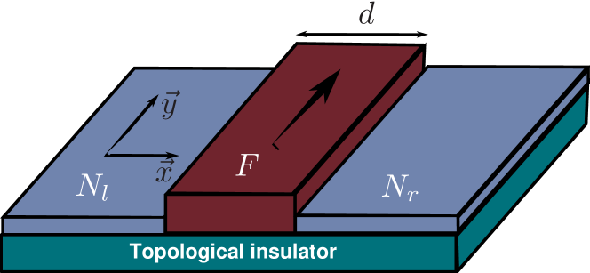
Figure 1: (Color online) Sketch of the N_lFN_r junction on the surface of a topological insulator. Pumping is induced by applying gate voltages (not shown) to the normal leads. In the middle region a thin ferromagnetic film induces ferromagnetism on the surface of the topological insulator by means of the exchange coupling Yokoyama2010 . The arrow in the middle region indicates the direction of the magnetization $M$ in this region.

We first describe the NFN junction, see Fig. 1. The junction is divided into three regions: region $N_{l}$ (for $x<0$), region $N_{r}$ (for $x>d$) and the ferromagnetic region $F$ in the middle. The left and right-hand side of the junction represent the bare topological insulator. The charge carriers (surface Dirac fermions) in these regions are described by the Hamiltonian $\mathcal{H}_{0}$ [Eq. (1)] whose eigenstates are given by

$$\psi_{N}^{\pm}=\frac{1}{\sqrt{2}}\,\left(\begin{array}[]{c}1\\ \pm e^{\pm i\alpha}\\ \end{array}\right)e^{\pm ik_{n}x}e^{iqy},$$ (2)

where $+(-)$ labels the wavefunctions traveling from the left (right) to the right (left) of the junction. The angle of incidence $\alpha$ and the momentum $k_{n}$ in the $x$-direction are given by:

$$\sin(\alpha)=\frac{\hbar v_{F}q}{|\epsilon+\mu|},$$ (3)

$$k_{n}=\sqrt{\left(\frac{\epsilon+\mu}{\hbar v_{F}}\right)^{2}-q^{2}}.$$ (4)

Here $\epsilon$ represents the energy measured from the Fermi energy $\epsilon_{F}$ and $q$ denotes the momentum in the $y$-direction. In the normal regions $N_{l}$ and $N_{r}$ a dc electrical voltage can be applied via metallic top gates to tune the chemical potential $\mu$ and thereby control the number of charge carriers incident on the junction. We assume gate voltages to be small compared to the bandgap for bulk states ($eV_{i}\ll E_{g}\sim 1$ eV, $i=l,r$), so that transport is well described by surface Dirac states HZhang2009 . In this case, the eigenstates are given by

$$\psi_{N_{l}}^{\pm}=\frac{1}{\sqrt{2}}\,\left(\begin{array}[]{c}1\\ \pm e^{\pm i\alpha_{l}}\\ \end{array}\right)e^{\pm ik_{n_{l}}x}e^{iqy},$$ (5)

$$\psi_{N_{r}}^{\pm}=\frac{1}{\sqrt{2}}\,\left(\begin{array}[]{c}1\\ \pm e^{\pm i\alpha_{r}}\\ \end{array}\right)e^{\pm ik_{n_{r}}(x-d)}e^{iqy},$$ (6)

$$\sin(\alpha_{i})=\frac{\hbar v_{F}q}{|\epsilon+\mu-eV_{i}|},$$ (7)

$$k_{n_{i}}=\sqrt{\left(\frac{\epsilon+\mu-eV_{i}}{\hbar v_{F}}\right)^{2}-q^{2}},$$ (8)

where the index $i=l,r$ labels the normal sides of the junction.

In the middle region M of the junction ($0<x<d$), the presence of the ferromagnetic strip modifies the Hamiltonian by providing an exchange field. The Hamiltonian that describes the surface states is now $\mathcal{H}=\mathcal{H}_{0}+\mathcal{H}_{\textrm{induced}}$, where the induced exchange Hamiltonian is given by Yokoyama2010 ; Mondal2010b

$$\mathcal{H}_{\textrm{induced}}=\hbar v_{F}M\sigma_{y},$$ (9)

with the magnetization $\vec{M}=M\hat{y}$. The magnitude $M$ depends on the strength of the exchange coupling of the ferromagnetic film and can be tuned for soft ferromagnetic films by applying an external magnetic field Yokoyama2010 . The eigenstates of the full Hamiltonian $\mathcal{H}$ are then given by:

$$\psi_{F}^{\pm}=\frac{1}{\sqrt{2}}\,\left(\begin{array}[]{c}1\\ \pm e^{\pm i\alpha_{m}}\\ \end{array}\right)e^{\pm ik_{m}x}e^{iqy},$$ (10)

with

$$\sin(\alpha_{m})=\frac{\hbar v_{F}(q+M)}{|\epsilon+\mu|},$$ (11)

and

$$k_{m}=\sqrt{\left(\frac{\epsilon+\mu}{\hbar v_{F}}\right)^{2}-(q+M)^{2}}.$$ (12)

From Eq. (12) we see that for a given energy there exists a critical magnetization

$$M_{c}=\pm\,2|\epsilon+\mu|/(\hbar v_{F}),$$ (13)

beyond which for all transverse ($q$) modes the wavefunction changes from propagating to spatially decaying (evanescent) along the $x$-direction Mondal2010a ; Mondal2010b .

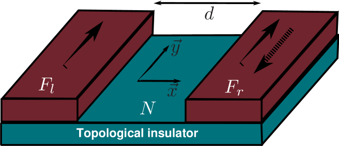
Figure 2: (Color online) Sketch of the F_lNF_r junction. Ferromagnetic films are placed on top of the topological insulator on the left and right providing exchange fields in these regions. The arrows indicate the direction of the corresponding magnetizations $M_{l}$ and $M_{r}$, see the text for further explanation.

Now we describe the FNF junction, see Fig. 2. Region $F_{l}$ ($x<0$) and region $F_{r}$ ($x>d$) are modeled as ferromagnetic regions, respectively, with different magnetizations $M_{l}$, $M_{r}$ along the $y$-axis and corresponding wavefunction $\psi_{F}$ [Eq. (10)]. The Dirac fermions in the middle region N ($0<x<d$) are described by the wavefunctions $\psi_{N}$ [Eq.(2)]. When calculating transport properties of the FNF junction, we focus on two different alignments of the magnetizations of the ferromagnetic regions: the parallel configuration (M_l $\parallel$ M_r), where the magnetizations in the ferromagnetic regions point in the same direction, and the anti-parallel configuration (M_l $\parallel$ - M_r), in which the magnetizations are in opposite directions.

Using Eqns. (2)-(12) we can calculate the reflection and transmission coefficients for a Dirac fermion with energy $\epsilon$ and transverse momentum $q$ incident from the left on the junction, for both the NFN and the FNF junctions. To this end, we consider a general F_lF_mF_r junction, where the wavefunctions in each of the three regions left ($l$), middle ($m$) and right ($r$) are given by:

$$\psi_{l} = \psi_{l}^{+}+r_{ll}\,\psi_{l}^{-},$$

$$\psi_{m} = p\,\psi_{m}^{+}+q\,\psi_{m}^{-},$$ (14)

$$\psi_{r} = t_{rl}\,\psi_{r}^{+}.$$

Here $\psi_{j}^{\pm}$ ($j=l,m,r$) are the wavefunctions (5), (6) or (10) (depending on the junction considered) and $r_{ll}$ and $t_{rl}$ denote the corresponding reflection and transmission coefficients. By requiring continuity of the wavefunction at the interfaces $x=0$ and $x=d$, we obtain the reflection and transmission coefficients:

$$r_{ll} = e^{i\alpha_{l}}\,\frac{e^{2ik_{m}d}(1+e^{i(\alpha_{m}+\alpha_{l})})(e^{i\alpha_{m}}-e^{i\alpha_{r}})+(e^{i\alpha_{l}}-e^{i\alpha_{m}})(1+e^{i(\alpha_{m}+\alpha_{r})})}{e^{2ik_{m}d}(e^{i\alpha_{m}}-e^{i\alpha_{l}})(e^{i\alpha_{m}}-e^{i\alpha_{r}})+(1+e^{i(\alpha_{m}+\alpha_{l})})(1+e^{i(\alpha_{m}+\alpha_{r})})},$$ (15)

$$t_{rl} = \frac{e^{ik_{m}d}(1+e^{2i\alpha_{m}})(1+e^{2i\alpha_{l}})}{e^{2ik_{m}d}(e^{i\alpha_{m}}-e^{i\alpha_{l}})(e^{i\alpha_{m}}-e^{i\alpha_{r}})+(1+e^{i(\alpha_{m}+\alpha_{l})})(1+e^{i(\alpha_{m}+\alpha_{r})})}.$$ (16)

Here $\alpha_{j}$ denotes the polar angle of the wavevector in region $j=l,m,r$ [Eqns. (7) and (11)]. When considering an electron incident from the right lead, one can similarly obtain $r_{rr}$ and $t_{lr}$. These expressions for the reflection and transmission coefficients form the basis of our calculations of the conductance and the pumped current in Secs. III and IV respectively.

III Conductance

The conductance $G^{\text{NFN}}$ of a topological insulator NFN junction has been studied in earlier work by Mondal et al. Mondal2010a ; Mondal2010b , who predicted oscillatory behavior of $G^{\text{NFN}}$ as a function of the applied bias voltage (see also Fig. 3). In this section we first briefly review their results and then add a quantitative explanation for the oscillations of the conductance. This explanation is crucial for understanding the behavior of the pumped current in the next section. We also calculate and analyze the conductance in a FNF junction.

The general expression for the conductance $G$ across the junction in terms of the transmission probability $T(\alpha)\equiv|t_{rl}(\alpha)|^{2}$ is given by

$$G=(G_{0}/2)\int_{-\pi/2}^{\pi/2}T(\alpha)\cos\alpha\,d\alpha.$$ (17)

Here $G_{0}=\frac{2e^{2}}{h}\rho(eV)\hbar v_{F}W$, $\rho(eV)=|\mu+eV|/(2\pi(\hbar v_{F})^{2})$ denotes the density of states, $W$ is the sample width, and the integration is over all the angles of incidence $\alpha$. For $V_{l}=V_{r}=0$ ($\alpha_{l}=\alpha_{r}=\alpha$) the angle-dependent transmission probability $T^{\text{NFN}}(\alpha)$ is given by Mondal2010a ; Mondal2010b

$$T^{\text{NFN}}(\alpha) = \cos^{2}(\alpha)\cos^{2}(\alpha_{m})/\left[\cos^{2}(k_{m}d)\cos^{2}(\alpha)\cos^{2}(\alpha_{m})\right.$$ (18)

$$\left.+\sin^{2}(k_{m}d)(1-\sin(\alpha)\sin(\alpha_{m}))^{2}\right],$$

where $\alpha_{m}$ is the polar angle of the wave vector in the middle region as defined in Eq. (11). This angle can be expressed in terms of $\alpha$ using the fact that the momentum is conserved along $y$-axis as:

$$\sin(\alpha_{m})=\sin(\alpha)+\frac{M\hbar v_{F}}{\mid\epsilon+\mu\mid}.$$ (19)

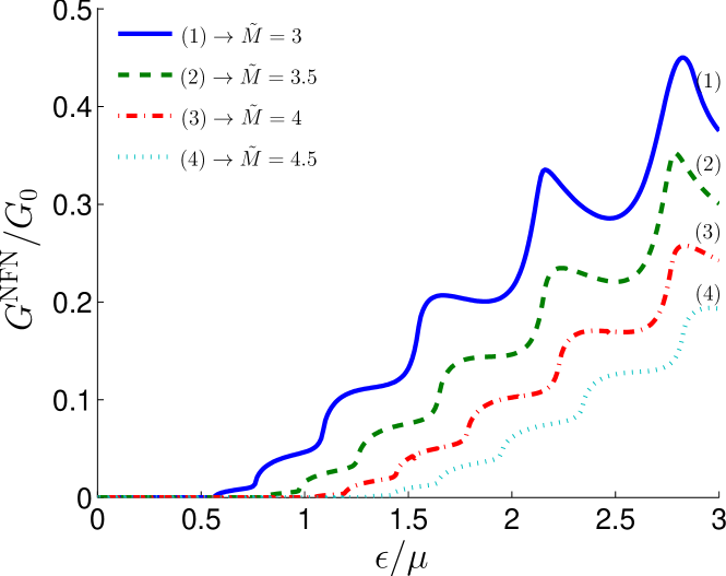
Figure 3: (Color online) The conductance $G^{\text{NFN}}$ of the NFN junction [Eq.(17)] as a function of $\epsilon/\mu$ for $V_{l}=V_{r}=0$ and for different values of the effective magnetization $\tilde{M}\equiv\hbar v_{F}M/\mu=3$ (solid blue line), 3.5 (dashed green line), 4 (dot-dashed red line) and 4.5 (dotted light-blue line). The effective junction width $\tilde{d}\equiv\mu d/(\hbar v_{F})=5$.

Figure 3 shows the conductance of the NFN junction [obtained from Eqns. (17) and (18)] as a function of the energy of the incoming carriers $\epsilon/\mu$ for different values of the effective magnetization $\tilde{M}\equiv\hbar v_{F}M/\mu$. For a given magnetization $M$, the conductance is zero for $\epsilon<\epsilon_{c}$, i.e., $G^{\text{NFN}}(\epsilon)=0$, with the critical energy $\epsilon_{c}\equiv\hbar v_{F}M/2-\mu$. Below this energy there are no traveling modes inside the barrier. Our results agree with the previous results in the literature Mondal2010a ; Mondal2010b .

From Fig. 3 it can be observed that the conductance changes from plateau-like to oscillatory as $\epsilon/\mu$ increases. In order to provide an explanation for this behavior we first analyze the plateau like regime in detail. After setting $\alpha_{l}=\alpha_{r}\equiv\alpha$ in Eq. (15), we begin by finding the conditions when the reflection coefficient is zero, i.e., $r_{ll}=0$. The first, trivial, condition $\alpha=\alpha_{m}+2\pi n$ corresponds to the situation of an entirely normal junction (i.e., no ferromagnetic region). The second and more interesting condition is $\sin(k_{m}d)=0$. This is the case when transmission occurs via a resonant mode of the junction and can be written as (using Eqns. (3) and (12))

$$k_{m}d=\frac{|\epsilon+\mu|}{\hbar v_{F}}d\sqrt{1-\left(\sin\alpha+\frac{\hbar v_{F}M}{|\epsilon+\mu|}\right)^{2}}=n\pi.$$ (20)

Eq. (20) indicates that for a given $M$ and $\epsilon$ there are certain privileged angles $\alpha_{c}$ for which the barrier becomes transparent:

$$\sin(\alpha_{c})=\pm\sqrt{1-\left(\frac{n\pi}{\tilde{d}(1+\frac{\epsilon}{\mu})}\right)^{2}}-\frac{\tilde{M}}{|1+\frac{\epsilon}{\mu}|},$$ (21)

with $\tilde{d}\equiv d\mu/(\hbar v_{F})$ being the dimensionless barrier length. These modes are referred to as resonant modes in this article.

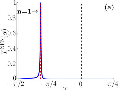
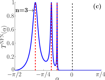
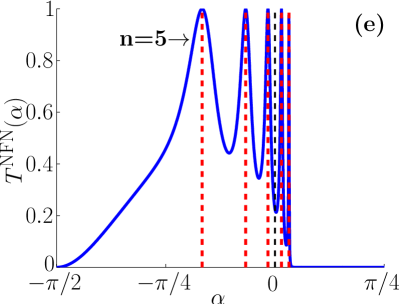
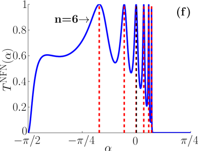
Figure 4: (Color online) The transmission probability $T^{\text{NFN}}(\alpha)$ [Eq. (18)] as a function of the angle of incidence $\alpha$ for different values of energy $\epsilon/\mu$, (a) $\epsilon/\mu=0.7$, (b) $\epsilon/\mu=0.9$, (c) $\epsilon/\mu=1.2$, (d) $\epsilon/\mu=1.6$, (e)$\epsilon/\mu=2.4$, and (f) $\epsilon/\mu=2.9$. Parameters used are $\tilde{d}=5$ and $\tilde{M}=3$.

Figure 4 shows the transmission probability [Eq. (18)] as a function of the angle of incidence $\alpha$ for different values of energy $\epsilon/\mu$. The dashed (red) vertical lines correspond to the angles satisfying Eq. (21) for different $n$. It can be seen that as the energy increases more resonant modes become available for transmission. It is also worth noting that for energies at which only one mode is present ($n=1$, see Fig. 4(a)) the transmission is strongly localized at one particular angle. This property could be exploited to fabricate single-mode filters. For low energy excitations only negative angles $\alpha$ (i.e., $q$-momenta anti-parallel to M) contribute to the conductance, see Figs. 4(a)-(d). As the energy increases, the resonant modes move from the left to the right and also positive angles $\alpha$ (i.e., $q$-momenta parallel to M) begin to contribute, see Figs. 4(e) and (f).

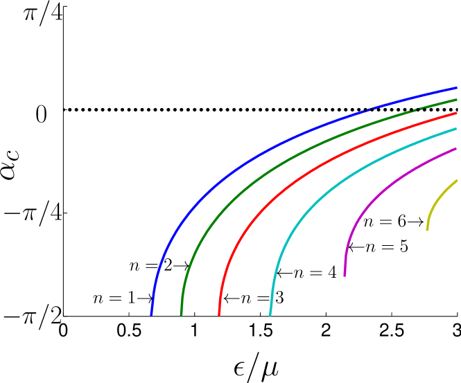
Figure 5: (Color online) The real part of the angle of incidence $\alpha_{c}$ [Eq. (21)] versus energy $\epsilon/\mu$ for the modes $n=1,2,3,4,5$. Parameters used are the same as in Fig. 4.

Now we address the question why a mode becomes resonant in the barrier. Figure 5 shows the angle of incidence $\alpha_{c}$ [Eq. (21)] for different values of $n$ as a function of energy $\epsilon/\mu$. For a given $n$, the resonant mode does not contribute to the conductance if the energy $\epsilon$ satisfies the condition $\epsilon_{c}<\epsilon<\epsilon_{c}^{\alpha_{n}}$, because the imaginary part of the momentum $k_{m}$ is nonzero and thus the mode is decaying along the $x$-direction. This critical energy $\epsilon_{c}^{\alpha_{n}}$ for each mode is given by:

$$\frac{\epsilon_{c}^{\alpha_{n}}}{\mu}=\frac{n^{2}\pi^{2}}{2\tilde{d}^{2}\tilde{M}}+\frac{\tilde{M}}{2}-1.$$ (22)

When $\epsilon>\epsilon_{c}^{\alpha_{n}}$, $k_{m}$ becomes real and the mode becomes resonant. As we increase the energy, all the modes asymptotically reach their saturation angle $\alpha=\pi/2$.

Finally, we analyze the effect of the appearance of subsequent resonant modes on the conductance. For small energies, the conductance increases in plateau-like steps (see Fig. 3). The first plateau corresponds to the situation in which the first transmission mode appears at $\alpha=-\pi/2$. As the energy increases, a new resonant mode appears and the conductance increases in a step-like manner. The plateaus are not sharp due to the fact that each new mode appearing is not sharply peaked, but rather has a certain distribution around a particular angle of incidence, see Fig. 4. Once the energy is large enough for there to be contributions from both positive and negative angles of incidence, the conductance becomes oscillatory. For very large energies ($\epsilon\gg\epsilon_{c}$), the effect of the magnetic barrier disappears and the conductance becomes unity ($G^{\text{NFN}}=G_{0}$).

Figure 6: (Color online) The conductance $G^{\text{NFN}}$ of the NFN junction as a function of $\epsilon/\mu$ for different values of gate voltages, $eV/\mu=0$ (solid blue line), 1 (dashed green line), 2 (dashed-dot red line) and 3 (double-dotted light-blue line). As before, $\tilde{M}=3$ and $\tilde{d}=5$.

Figure 6 shows the conductance as a function of energy for several values of applied bias voltages $V_{l}=V_{r}\equiv V$. As expected, the features of the conductance remain the same for finite $V$. As we increase $eV$, the critical energy $\epsilon_{c}=\hbar v_{F}M/2+eV/2-\mu$ for the onset of the conductance increases and the spacing between two consecutive resonant modes decreases. As a result the plateaus become narrower.

In the remaining part of this section we study the conductance in a topological insulator FNF junction, as shown in Fig. 2. We consider both the junction with parallel and with anti-parallel magnetization in the ferromagnetic regions. In the parallel configuration, using $\alpha_{l}=\alpha_{r}\equiv\alpha=\sin^{-1}(\hbar v_{F}(q+M)/|\epsilon+\mu|)$ and $\alpha_{m}=\sin^{-1}(\hbar v_{F}q/|\epsilon+\mu|)$ in Eq. (16), we find that the conductance is similar to the conductance of a NFN junction, as displayed in Fig. 3. However, in the FNF junction the first resonant mode becomes resonant for positive $\alpha$ (i.e., transverse $q$-momentum parallel to $M$) and as the energy increases, the resonances move towards negative values of the angle $\alpha$. This, however, does not affect the total conductance, as we sum over all possible angles of incidence, and the same analysis as for the NFN junction presented above can be applied to understand the FNF junction with parallel magnetization.

In the case of anti-parallel alignment of the magnetization in the two ferromagnetic regions, we substitute $\sin(\alpha_{l})=\hbar v_{F}(q+M)/|\epsilon+\mu|$, $\sin(\alpha_{r})=\hbar v_{F}(q-M)/|\epsilon+\mu|$ and $\sin(\alpha_{m})=\hbar v_{F}q/|\epsilon+\mu|$ in Eq. (16). The conductance of this junction was studied previously in Refs. Wu2010 ; Salehi2011 and the transmission probability $T^{\text{FNF,AP}}(\alpha_{l},\alpha_{r})\equiv|t_{rl}(\alpha_{l},\alpha_{r})|^{2}$ is given by:

$$T^{\text{FNF,AP}}(\alpha_{l},\alpha_{r})=\frac{\cos^{2}(\alpha_{l})\cos^{2}(\alpha_{m})}{\cos^{2}(k_{m}d)\cos^{2}(\frac{\alpha_{l}+\alpha_{r}}{2})\cos^{2}(\alpha_{m})+\sin^{2}(k_{m}d)\left[\cos\left(\frac{\alpha_{l}-\alpha_{r}}{2}\right)-\sin(\frac{\alpha_{l}+\alpha_{r}}{2})\sin(\alpha_{m})\right]^{2}}.$$ (23)

The total conductance is obtained by multiplying $T^{\text{FNF,AP}}(\alpha_{l},\alpha_{r})$ with $\cos(\alpha_{r})/\cos(\alpha_{l})$ and then integrating over the allowed angles of incidence restriction , i.e., from $\alpha_{c_{1}}=\sin^{-1}(2\hbar v_{F}M/(|\epsilon+\mu|)-1)$ to $\alpha_{c_{2}}=\sin^{-1}(2\hbar v_{F}M/(|\epsilon+\mu|)+1)$. Thus we can write

$$G^{\text{FNF,AP}}=G_{0}/2\int_{\alpha_{c_{1}}}^{\pi/2}G^{\text{FNF,AP}}(\alpha_{l},\alpha_{r})\cos(\alpha_{l})d\alpha_{l},$$ (24)

where

$$G^{\text{FNF,AP}}(\alpha_{l},\alpha_{r})=\frac{\cos(\alpha_{r})}{\cos(\alpha_{l})}T^{\text{FNF,AP}}(\alpha_{l},\alpha_{r}).$$ (25)

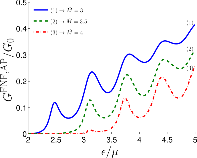
Figure 7: (Color online) The conductance $G^{\text{FNF,AP}}$ of the FNF junction in the anti-parallel configuration as a function of $\epsilon/\mu$, for $\tilde{M}=3$ (blue solid line), $3.5$ (green dashed line) and $4$ (red dotted line). The parameter $\tilde{d}=5$.

Fig. 7 shows the conductance of the FNF junction in the anti-parallel configuration. From the horizontal axis we see that the critical energy $\epsilon_{c}$ for the onset of the conductance is larger than in the corresponding parallel configuration. Moreover, as the energy $\epsilon/\mu$ increases the conductance exhibits no plateau behavior: it increases in an oscillatory fashion. This oscillatory behavior can be understood from Fig. 8, which shows $G^{\text{FNF,AP}}(\alpha)$ for four different values of $\epsilon/\mu$. Note that all the angles ($\alpha_{l}$, $\alpha_{m}$ and $\alpha_{r}$) can be expressed in terms of one angle, which we choose to be $\alpha_{l}\equiv\alpha$. As the energy increases, the area under the curve oscillates resulting in oscillations in the conductance.

Summarizing, we have obtained a quantitative explanation for the behavior of the conductance in topological insulator NFN and FNF-junctions in terms of the number of resonant modes in the junction. This explanation forms the basis for understanding the behavior of the pumped current in the next section.

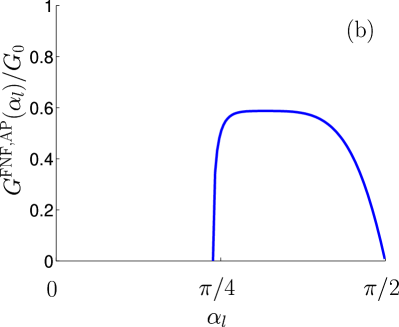
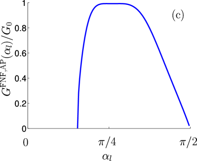
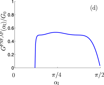
Figure 8: The angle-dependent total transmission $T^{\text{FNF,AP}}(\alpha_{l},\alpha_{r})$ for the anti-parallel configuration of the FNF junction as a function of the angle of incidence $\alpha_{l}$ for (a) $\epsilon/\mu=2.47$, (b) $\epsilon/\mu=2.57$, (c) $\epsilon/\mu=3.10$ and (d) $\epsilon/\mu=3.40$. Parameters used are $\tilde{M}=3$ and $\tilde{d}=5$.

IV Adiabatically pumped current

In this section we investigate adiabatically pumped currents through NFN and FNF junctions in a topological insulator difference . In general, a pumped current is generated by slow variation of two system parameters $X_{1}$ and $X_{2}$ in the absence of a bias voltage Buttiker1994 ; Brouwer1998 . For periodic modulations $X_{1}(t)=X_{1,0}+\delta X_{1}\cos(\omega t)$ and $X_{2}(t)=X_{2,0}+\delta X_{2}\cos(\omega t+\phi)$, the pumped current $I_{p}$ into the left lead of the junction can be expressed in terms of the area $A$ enclosed by the contour that is traced out in $(X_{1},X_{2})$-parameter space during one pumping cycle as Brouwer1998 :

$$I_{p} = \frac{\omega e}{2\pi^{2}}\int_{A}\,dX_{1}\,dX_{2}\,\sum_{m}\ \Pi(X_{1},X_{2})$$ (26a)

$$\approx \frac{\omega e}{2\pi}\,\delta X_{1}\,\delta X_{2}\,\sin\phi\,\sum_{m}\ \Pi(X_{1},X_{2}),$$ (26b)

with

$$\Pi(X_{1},X_{2})\equiv\mbox{\rm Im}\ \left(\frac{\partial r_{ll}^{\ast}}{\partial X_{1}}\frac{\partial r_{ll}}{\partial X_{2}}+\frac{\partial t_{lr}^{\ast}}{\partial X_{1}}\frac{\partial t_{lr}}{\partial X_{2}}\right).$$ (27)

Here $r_{ll}$ and $t_{lr}$ represent the reflection and transmission coefficients into the left lead and the index $m$ sums over all modes (a similar expression can be obtained for the pumped current into the right lead). Eq. (26b) is valid in the bilinear response regime where $\delta X_{1}\ll X_{1,0}$ and $\delta X_{2}\ll X_{2,0}$ and the integral in Eq. (26a) becomes independent of the pumping contour.

First we analyze the NFN pump, where the pumped current is generated by adiabatic variation of gate voltages $V_{l}$ and $V_{r}$ which change the chemical potential in the normal leads on the left and right of the junction, respectively (see Fig. 1). Calculating the derivatives of the reflection and transmission coefficients $r_{ll}$ [Eq. (15)] and $t_{rl}$ with respect to $\alpha_{l}$ and $\alpha_{r}$, substituting into Eq. (27) and using $\partial\alpha_{j}/(e\partial V_{j})=\tan(\alpha_{j})/|\epsilon+\mu-eV_{j}|$ ($j=l,r$), the pumped current for $V_{1}=V_{2}\equiv V$ and for a specific angle of incidence $\alpha$ is given by:

$$I_{p}^{\text{NFN}}(\alpha)=-I_{0}^{\text{NFN}}\frac{\cos^{3}(\alpha_{m})\sin^{2}(\alpha)\cos(\alpha)\sin(2k_{m}d)}{(1+\epsilon/\mu-eV/\mu)^{2}(\cos^{2}(\alpha)\cos^{2}(\alpha_{m})\cos^{2}(k_{m}d)+\sin^{2}(k_{m}d)(1-\sin(\alpha)\sin(\alpha_{m}))^{2})^{2}}.$$ (28)

Here $I_{0}^{\text{NFN}}\equiv\omega e/(8\pi)\sin({\phi})(e\delta V_{1}/\mu)(e\delta V_{2}/\mu)$ and $\sin(\alpha_{m})$ is given by Eq. (19). In the limit $M\rightarrow 0$ (i.e., $\alpha_{m}\rightarrow\alpha$) in an entirely normal junction, we obtain from Eq. (28) the angle-dependent pumped current as:

$$I_{p}^{\text{NFN}}|_{\tilde{M}=0}=I_{0}^{\text{NFN}}\int_{-\pi/2}^{\pi/2}\frac{\sin(2k_{m}d)\sin^{2}\alpha}{(1+\epsilon/\mu-eV/\mu)\cos^{3}\alpha}\,d\alpha.$$ (29)

On the other hand, the transmission $T^{\text{NFN}}(\alpha)$ [Eq. (18)] in this limit is given by $T^{\text{NFN}}|_{\tilde{M}\rightarrow 0}\rightarrow 1$, independent of the angle of incidence $\alpha$. We notice that even if the probability for transmission is one, it is possible to pump a current in the adiabatic driving regime. The total pumped current $I_{p}^{NFN}$ is then obtained by integrating over $\alpha$:

$$I_{p}^{\text{NFN}}=\int_{-\pi/2}^{\pi/2}I_{p}^{\text{NFN}}(\alpha)\cos\alpha\,d\alpha.$$ (30)

In general, this integral cannot be evaluated analytically and we have obtained our results numerically.

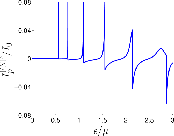
Figure 9: The pumped current $I_{p}^{\text{NFN}}$ [Eq. (30)] in the NFN junction as a function of $\epsilon/\mu$ for $V=0$, $\tilde{d}=5$ and $\tilde{M}=3$.

Figure 9 shows the total pumped current $I_{p}^{\text{NFN}}$ (in units of $I_{0}^{\text{NFN}}$) at zero bias $V=V_{1}=V_{2}=0$ for $\tilde{M}=3$. Comparing Figs. 3 and 9 we see that there is a correlation between the pumped current and the conductance for the NFN junction: for low energies, the pumped current $I_{p}^{NFN}$ is zero as no traveling modes are allowed in the junction. As we increase the energy, each time a resonant mode appears [see Eq. (20)], the pumped current diverges and changes sign. For energies where both positive and negative angles of incidence contribute to the conductance, the pumped current remains finite but keeps changing its sign. From Figs. 3 and 9 it can also be seen that the pumped current vanishes for energies at which subsequent resonant modes become fully transmitting. In order to gain further insight we plot the analogue of Fig. 4 for the pumped current. Figure  10 shows the pumped current [Eq. 30] as a function of the angle of incidence $\alpha$ for different values of $\epsilon/\mu$. The chosen values of $\epsilon/\mu$ are same as in Fig. 4. We see that the features in Fig. 10 have a direct correlation with the features in Fig. 4: whenever there is a sharp peak in the transmission the pumped current diverges and changes sign. The key feature that distinguishes between the pumped current and the conductance is that the pumped current changes sign at particular values of the energy, while the conductance does not.

Now we analyze the pumped current in the FNF junction with parallel orientation of the magnetizations. In this system, the driving parameters are the magnetizations $M_{l}$ and $M_{r}$ in the left and right contacts, respectively, see Fig. 2. After calculating the derivatives of the reflection and transmission coefficients, obtaining the imaginary part of Eq. (27), and using $\partial\alpha_{j}/\partial M_{j}=\hbar v_{F}/(|\epsilon+\mu|\cos(\alpha_{j}))$ ($j=l,r)$, the pumped current $I_{p}^{\text{FNF}}(\alpha)$ for $M_{1}=M_{2}=M$ is:

$$I_{p}^{\text{FNF}}(\alpha)=-I_{0}^{\text{FNF}}\frac{\cos^{3}(\alpha_{m})\cos(\alpha)\sin(2k_{m}d)}{(1+\epsilon/\mu)^{2}(\cos^{2}(\alpha)\cos^{2}(\alpha_{m})\cos^{2}(k_{m}d)+\sin^{2}(k_{m}d)(1-\sin(\alpha)\sin(\alpha_{m}))^{2})^{2}}.$$ (31)

Here $I_{0}^{\text{FNF}}=\omega e/(8\pi)\sin({\phi})(\hbar v_{F}\delta M_{l}/\mu)(\hbar v_{F}\delta M_{r}/\mu)$ and $\sin(\alpha_{m})=\sin(\alpha)-\hbar v_{F}M/(|\epsilon+\mu|)$.

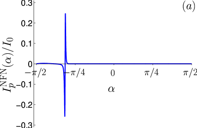
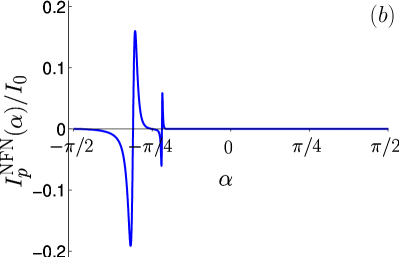
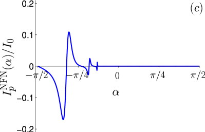
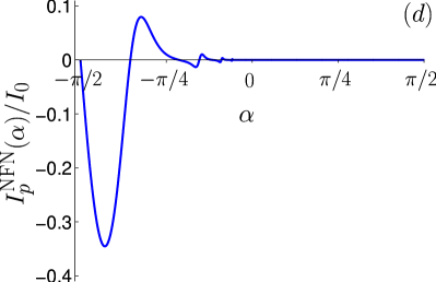
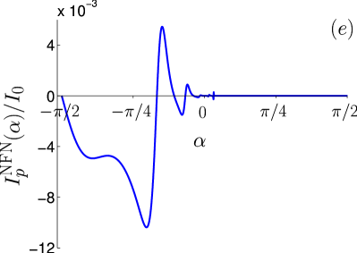
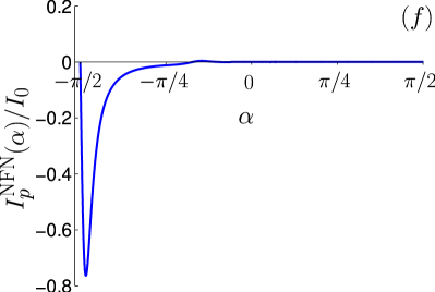
Figure 10: The pumped current $I_{p}^{\text{NFN}}(\alpha)$ [Eq. (28)] as a function of the angle of incidence $\alpha$ for different values of energy $\epsilon/\mu$, (a) $\epsilon/\mu=0.7$, (b) $\epsilon/\mu=0.9$, (c) $\epsilon/\mu=1.2$, (d) $\epsilon/\mu=1.6$, (e) $\epsilon/\mu=2.4$, and (f) $\epsilon/\mu=2.9$. Parameters used are $\tilde{d}=5$ and $\tilde{M}=3$.

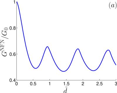
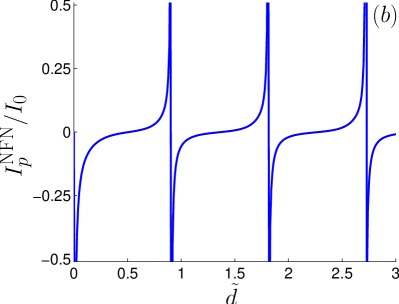
Figure 11: (a) The conductance of the NFN junction as a function of $\tilde{d}$. (b) The pumped current for the NFN junction as a function of $\tilde{d}$. Parameters used are $\epsilon/\mu=2.5$, $\tilde{M}=3$ and $V=0$.

The behavior of the current $I_{p}^{\text{FNF}}$ is similar to that of the pumped current $I_{p}^{\text{NFN}}$ in a NFN-junction (shown in Fig. 9). This can also be seen by comparing the denominators in Eqns. (28) and (31). Again we observe that the pumped current diverges at exactly the same locations where the conductance changes sharply. But there is an important difference between both pumped currents. The pumped current in an NFN-junction at normal incidence vanishes, $I_{p}^{\text{NFN}}(\alpha=0)=0$, while $I_{p}^{\text{FNF}}(\alpha=0)\neq 0$. This difference arises because the two pumps are driven by two different parameters (voltages in the NFN pump and magnetizations in the FNF pump).

Finally, we briefly analyze the behavior of the pumped current as a function of the width $d$ of the middle region. For energies below $\epsilon_{c}$, the pumped current of the NFN junction decays to zero as the width $d$ increases (there are no resonant modes in the system). For energies larger than $\epsilon>\epsilon_{c}$, the pumped current $I_{p}^{\text{NFN}}$ oscillates as a function of width $\tilde{d}$. Fig. 11 shows the conductance and the pumped current as a function of $\tilde{d}$ for $\epsilon/\mu=2.5$. The peaks in the conductance correspond to the resonance condition Eq. (20). The pumped current $I_{p}^{\text{NFN}}$ changes its sign at exactly the same values of $\tilde{d}$ where the conductance has a maximum. This analysis holds as well for the FNF junction.

V Summary and discussion

To summarize, we have analyzed quantum transport by Dirac fermion surface states in NFN and the FNF junctions in a 3D topological insulator. We have shown that for low energies the appearance of a new resonant mode results in a plateau-like increment of the conductance and a diverging pumped current in these junctions which also changes sign. This is our key result, and represents an experimentally distinguishable signature between conductance and the pumped current. We highlighted an interesting difference between the two different pumping mechanisms for the NFN and FNF junctions, observing different behaviors for normal incidence ($\alpha=0$). Experimentally, the NFN pump could be realized using current technology. The FNF pump will be more difficult to realize since it requires oscillating magnetizations. A possible way to realize a FNF pump could be by moving the two ferromagnetic layers coherently using a nanomechanical oscillator Kovalev2005 . Experimental verification of our predictions will provide further insight into quantum transport through these junctions.

- (1) M. Z. Hasan and C. L. Kane, Rev. Mod. Phys. 82, 3045 (2010).
- (2) M. König, S. Wiedmann, C. Brüne, A. Roth, H. Buhmann, L. W. Molenkamp, X.-L. Qi, and S.-C. Zhang, Science 318, 766 (2007).
- (3) D. Hsieh, D. Qian, L. Wray, Y. Xia, Y. S. Hor, R. J. Cava, and M. Z. Hasan, Nature 452, 970 (2008) .
- (4) Y. Xia, D. Qian, D. Hsieh, L. Wray, A. Pal, H. Lin, A. Bansil, D. Grauer, Y. S. Hor, R. J. Cava, and M. Z. Hasan, Nature Phys. 5, 398 (2009).
- (5) Y. Xia, D. Qian, D. Hsieh, R. Shankar, H. Lin, A. Bansil, A. V. Fedorov, D. Grauer, Y. S. Hor, R. J. Cava and M. Z. Hasan, arXiv:0907.3089.
- (6) D. Hsieh, Y. Xia, D. Qian, L. Wray, J. H. Dil, F. Meier, J. Osterwalder, L. Patthey, J. G. Checkelsky, N. P. Ong, A. V. Fedorov, H. Lin, A. Bansil, D. Grauer, Y. S. Hor, R. J. Cava, and M. Z. Hasan, Nature 460, 1101 (2009).
- (7) P. Roushan, J. Seo, C. V. Parker, Y. S. Hor, D. Hsieh, D. Qian, A. Richardella, M. Z. Hasan, R. J. Cava, and A. Yazdani, Nature 460, 1106 (2009).
- (8) D. Hsieh, Y. Xia, L. Wray, D. Qian, A. Pal, J. H. Dil, J. Osterwalder, F. Meier, G. Bihlmayer, C. L. Kane, Y. S. Hor, R. J. Cava, and M. Z. Hasan, Science 323, 919 (2009).
- (9) H. Zhang, Chao-Xing Liu, Xiao-Liang Qi, Xi Dai, Zhong Fang and Shou-Cheng Zhang, Nature Physics 5, 438 (2009).
- (10) L. Fu and C. L. Kane, Phys. Rev. Lett. 100, 096407 (2008).
- (11) T. Zhang, P. Cheng, X. Chen, J.-F. Jia, X. Ma, K. He, L. Wang, H. Zhang, X. Dai, Z. Fang, X. Xie, Q.-K. Xue, Phys. Rev. Lett. 103, 266803 (2009).
- (12) S. Mondal, D. Sen, K. Sengupta, and R. Shankar, Phys. Rev. Lett. 104, 046403 (2010).
- (13) S. Mondal, D. Sen, K. Sengupta, and R. Shankar, Phys. Rev. B 82, 045120 (2010).
- (14) Ya Zhang and Feng Zhai, Appl. Phys. Lett. 96, 172109 (2010).
- (15) T. Yokoyama, Y. Tanaka, and N. Nagaosa, Phys. Rev. B 81, 121401(R) (2010).
- (16) Zhenzua Wu, F. M. Peeters, and Kai Chang, Phys. Rev. B 82, 115211 (2010).
- (17) M. Salehi, M. Alidoust, Y. Rahnavard, and G. Rashedi, Physica E 43, 4, 966 (2011).
- (18) A. R. Akhmerov, J. Nilsson, and C. W. J. Beenakker, Phys. Rev. Lett. 102, 216404 (2009).
- (19) Y. Tanaka, T. Yokoyama, and N. Nagaosa, Phys. Rev. Lett. 103, 107002 (2009).
- (20) M. Büttiker, H. Thomas, and A. Prêtre, Z. Phys. B 94, 133 (1994).
- (21) P. W. Brouwer, Phys. Rev. B 58 10135(R) (1998).
- (22) B. Spivak, F. Zhou, and M. T. Beal Monod, Phys. Rev. B 51, 13226 (1995).
- (23) M. Switkes, C. M. Marcus, K. Campman, and A. D. Gossard, Science 283, 1905 (1999).
- (24) E. R. Mucciolo, C. Chamon, and C. M. Marcus, Phys. Rev. Lett. 89, 146802 (2002).
- (25) P. Sharma and P. W. Brouwer, Phys. Rev. Lett. 91, 166801 (2003).
- (26) S. K. Watson, R. M. Potok, C. M. Marcus, and V. Umansky, Phys. Rev. Lett. 91, 258301 (2003).
- (27) J. Splettstoesser, Michele Governale, J. König, and R. Fazio, Phys. Rev. Lett. 95, 246803 (2005).
- (28) E. Sela and Y. Oreg, Phys. Rev. Lett. 96 , 166802 (2006).
- (29) F. Reckermann, J. Splettstoesser, and M. R. Wegewijs, Phys. Rev. Lett. 104, 226803 (2010).
- (30) E. Prada, P. San-Jose, and H. Schomerus, Phys. Rev. B 80, 245414 (2009).
- (31) R. Zhu and H. Chen, Appl. Phys. Lett. 95, 122111 (2009).
- (32) E. Prada, P. San-Jose, and H. Schomerus, Solid State Commun. 151, 1065 (2011).
- (33) G. M. M. Wakker and M. Blaauboer, Phys. Rev. B, 82, 205432 (2010).
- (34) R. P. Tiwari and M. Blaauboer, Appl. Phys. Lett. 97, 243112 (2010).
- (35) M. Alos-Palop and M. Blaauboer, Phys. Rev. B 84, 073402 (2011).
- (36) A. Kundu, S. Rao, and A. Saha, Phys. Rev. B 83, 165451 (2011).
- (37) M. Blaauboer, Phys. Rev. B 68, 205316 (2003).
- (38) R. Citro, F. Romeo, and N. Andrei, ArXiv:1109.1711.
- (39) F. Giazotto, P. Spathis, S. Roddaro, S. Biswas, F. Taddei, M. Governale and L. Sorba, Nature Physics (2011).
- (40) This restriction of the angles of incidence comes from the fact that the minimum and the maximum value of the angle for the transmitted wavefunction is and respectively.
- (41) A fundamental difference between these pumps and the ones in graphene Prada2009 ; Zhu2009 ; Prada2010 ; Wakker2010 ; Tiwari2010 ; AlosPalop2011 is the nature of the spinor in the Hamiltonian (1) which in our case represents a real spin due to the spin-orbit interaction, while in graphene the spinor represents a pseudo-spin (or the sub-lattice variable).
- (42) A. A. Kovalev, G. E. W. Bauer, and A. Brataas, Phys. Rev. Lett. 94, 167201 (2005).