Improved convergence of scattering calculations in the oscillator representation.

Abstract

The Schrödinger equation for two and tree-body problems is solved for scattering states in a hybrid representation where solutions are expanded in the eigenstates of the harmonic oscillator in the interaction region and on a finite difference grid in the near– and far–field. The two representations are coupled through a high–order asymptotic formula that takes into account the function values and the third derivative in the classical turning points. For various examples the convergence is analyzed for various physics problems that use an expansion in a large number of oscillator states. The results show significant improvement over the JM-ECS method [Bidasyuk et al, Phys. Rev. C 82, 064603 (2010)].

1 Introduction

The accurate prediction of the breakup of a many-particle system into multiple fragments is one of the most challenging problems in quantum mechanics. Not only the relative motion of the particles needs to be modeled, but also the internal structure of the target and the products need to be described accurately. This leads in many cases, to a high–dimensional Schrödinger equation posed on a huge domain. For example, in breakup or collisions of nuclear clusters the cross section depends on a delicate interplay of the forces that hold the clusters together and the forces between the clusters.

The quantum state that describes the internal structure of a bound many particle system is often represented as linear combination of eigenstates of the quantum mechanical oscillator. These states form an $L^{2}$-basis which reduces the problem to finding the correct expansion coefficients. Examples are the correlated many electron state of a quantum dot [1, 2, 3] and the many nucleon state in nuclear physics [4, 5]. The various applications of the oscillator representation are discussed in [6]. Such a representation is very efficient for tightly bound ground state or lowest excited states as any smooth potential well is close to parabolic shape near it’s bottom. As a result, if the oscillator parameter is optimized to match this local parabolic potential, the lowest states of a system can be efficiently represented with only a few oscillator functions [7].

However, the representation is inefficient to describe scattering or break-up processes. Scattering states are not square integrable and many oscillator states are required to represent the interaction and asymptotic region. Furthermore, many potential matrix elements need to be calculated and this results in a dense linear system that has a complexity of $N^{3}$ to arrive at the solution, where $N$ is the number of oscillator states used in the representation, omitting the cost of calculating the potential matrix elements.

The $J$-matrix method offers a way of calculating cross sections and other scattering observables in the oscillator representation. It was proposed by Heller and Yamani in the seventies [8, 9] and mainly applied to atomic problems. The method exploits the tridiagonal structure of the kinetic energy operator. The $J$-matrix has been under constant development since its inception and a review of the recent developments can be found in [10]. For problems with Coulomb interactions the Coulomb-Sturmian basis is preferred over the oscillator representation. Recently the Coulomb-Sturmians have been used to describe multiphoton single and double-ionization [11] and electron impact ionization [12].

At the same time, and mostly independent, the Algebraic Resonating Group Method was developed for nuclear scattering problems [4, 13, 14, 15, 16]. This method exploits the same principles as the $J$-matrix method for description of nuclear cluster systems, where the oscillator representation is efficiently used to describe the internal structure of clusters. If the same representation is used for intercluster degrees of freedom, then the nucleon symmetrization rules become straightforward.

One shortcoming of the methods based on an $L^{2}$ basis is that the asymptotic solutions need to be known explicitly before a system for the wave function in the inner region and the scattering observables can be written down. This is a serious limitation since it is hard to find the asymptotic wave function for breakup reactions with multiple fragments. The Complex Scaling method, which scales the full domain into the complex plane, can be easily implemented in the oscillator representation by taking a complex valued oscillator strength. This has been used to calculate energy spectrum or extract the resonances [17], but the calculation of cross sections and other scattering observables may be quite difficult.

In recent decades significant progress has been made in the numerical solution of scattering processes described by the Helmholtz equation. In contrast to many particle systems, where the potential $V$ is often non-local, the wave number $k(x)$ in the Helmholtz equation depends only on the local material parameters such as the speed of sound in acoustics or the electric permittivity and magnetic permeability for electromagnetic scattering. For these problems grid based representations such as finite difference, finite element [18, 19], or Discontinuous Galerkin [20, 21] are preferred since they lead to sparse matrices that can be easily solved by preconditioned Krylov subspace methods [22, 23].

Another technique that has found widespread application is the use of absorbing boundary conditions. These boundary conditions allow a scattering calculation without prior knowledge about the asymptotic wave form. Exterior Complex Scaling (ECS) and Complex Scaling (CS) are widely used in atomic and molecular physics [24, 25, 26, 27]. Perfectly matched layers (PML) are used for electromagnetic and acoustic scattering [28], which can also be interpreted as a complex stretching transformation [29]. There are many other excellent absorbing boundary conditions [30, 31, 32].

In [33] the JM-ECS method was introduced that combines the $J$-Matrix method with a grid based ECS. The method describes the scattering solution in the interior region with an oscillator representation and in the exterior region with finite differences. The two representations are matched through a low order asymptotic formula with an error that scales as $\mathcal{O}(N^{-1/2})$, where $N$ is the size of the oscillator basis describing the inner region. Once the grid and oscillator representation are matched, it is easy to introduce an absorbing boundary layer since the grid representation can be easily extended with an ECS absorbing layer or any other absorbing boundary condition.

The resulting method was illustrated for one– and two–dimensional model problems representative for real scattering problems with local interactions. Furthermore, the representation was used for nuclear $p$-shell scattering. However, the accuracy of the calculations was unsatisfactory due the low–order matching condition. While the grid representation on the exterior has an accuracy of $\mathcal{O}(N^{-1})$, the matching is only accurate to order $\mathcal{O}(N^{-1/2})$.

The main contribution of the current paper is to increase the accuracy of the asymptotic formula that allows a better matching of the grid and oscillator representations. The better asymptotic formula takes function values and its third derivative into account. It can bring the matching error down to the level of the accuracy of the grid representation.

A higher–order asymptotic approximation of the oscillator representation was already discussed by S. Igashov in [34]. However, the formula was not used to increase the accuracy of scattering calculations.

This paper is outlined as followed. In Section 2 we shortly describe the process of scattering calculations in the oscillator representation. In Section 3 we derive a higher–order asymptotic formula that takes into account the behavior of the function in the classical turning points in coordinate and Fourier space. In Section 4 and 5 we use this asymptotic formula to solve scattering problems.

2 Review of scattering calculations in the oscillator representation

In this section we discuss the most important properties of the oscillator representation and how they can be used to perform scattering calculations with the $J$-matrix method. We also recall the working of the hybrid $J$-matrix and ECS method proposed in [33].

2.1 The radial scattering equation

The aim is to solve the Schrödinger equation in atomic units ($m=1$, $\hbar=1$) that describes a scattering process of two particles for an energy $E\in\mathbb{R}$. This equation written in relative coordinates is

$$\left[-\frac{1}{2}\Delta+V(\mathbf{r})-E\right]\Psi(\mathbf{r})=F(\mathbf{r}),\quad\forall\mathbf{r}\in\mathbb{R}^{3}$$ (1)

where $F(\mathbf{r})$ is the function describing the initial state or the source term and $V(\mathbf{r})$ is the potential. The coordinate $\mathbf{r}$ can be written in spherical coordinates $(\rho,\theta,\phi)$. In case of spherically symmetric potential ($V(\mathbf{r})=V(\rho)$), Eq. (1) can be reduced to a one-dimensional radial equation using partial wave decomposition

$$\Psi(\mathbf{r})=\Psi(\rho,\theta,\phi)=\sum_{l,m}\frac{\psi_{l}(\rho)}{\rho}Y_{l,m}(\theta,\phi),\quad F(\mathbf{r})=F(\rho,\theta,\phi)=\sum_{l,m}\frac{f_{l}(\rho)}{\rho}Y_{l,m}(\theta,\phi),$$

where $Y_{l,m}(\theta,\phi)$ is a spherical harmonic, $l=0,1,2,\ldots$ is the orbital angular momentum of the relative motion, $m$ is the projection of this angular momentum. The resulting reduced radial equation becomes

$$\left[-\frac{1}{2}\frac{d^{2}}{d\rho^{2}}+\frac{l(l+1)}{2\rho^{2}}+V(\rho)-E\right]\psi_{l}(\rho)=f_{l}(\rho).$$ (2)

For the problem we are interested in there is a range $a>0$ such that for all $\rho>a$ both $V(\rho)$ and $\chi(\rho)$ are zero.

We solve the Eq. (2) for $E>0$ and extract from the solution $\psi_{l}$ scattering observables such as the cross sections or phase shift. In order to solve the Eq. (2) we represent the solution as

$$\psi_{l}(\rho)=\sum_{n=0}^{\infty}c_{n,l}\varphi_{n,l}(\rho),$$ (3)

where $\varphi_{n,l}(\rho)$ are orthogonal $L^{2}$ functions, in particular we will use reduced oscillator functions, whose properties will be explained in the next section. After projection of (3) on $\varphi_{n,l}$, Eq. (2) results in an infinite linear system

$$\sum_{n=0}^{\infty}\left(T^{(l)}_{kn}+V^{(l)}_{kn}-E\right)c_{n,l}=b_{k,l},$$ (4)

where $T_{kn}^{(l)}$ denotes the elements of the kinetic energy matrix and $V_{kn}$ the elements of the potential energy matrix. They are the integrals

$$T^{(l)}_{kn}=\int_{0}^{\infty}\varphi_{k,l}(\rho)\left(-\frac{1}{2}\frac{d^{2}}{d\rho^{2}}+\frac{l(l+1)}{2\rho^{2}}\right)\varphi_{n,l}(\rho)\;d\rho,$$

$$V^{(l)}_{kn}=\int_{0}^{\infty}\varphi_{k,l}(\rho)V(\rho)\varphi_{n,l}(\rho)\;d\rho$$

and $b_{k,l}=\int_{0}^{\infty}\varphi_{k,l}(\rho)\chi_{l}(\rho)\;d\rho$. As the considered problem is effectively one-dimensional we will use $x$ instead of $\rho$ to denote radial relative coordinate in all following sections devoted to two-body problem.

2.2 The oscillator representation

Before we explain the strategy to solve Eq. (4), we repeat the main properties of the oscillator representation and the function $\varphi_{n,l}$ that will be used in the expansion.

The reduced radial equation analogous to (2) for the quantum harmonic oscillator with an oscillator strength $\omega$ is

$$\left[-\frac{1}{2}\frac{d^{2}}{dx^{2}}+\frac{1}{2}\frac{l(l+1)}{x^{2}}+\frac{1}{2}\omega^{2}x^{2}\right]\varphi_{n,l}(x)=E_{n,l}\varphi_{n,l}(x)$$ (5)

with $x\in[0,\infty[$ a radial coordinate. The boundary conditions are $\varphi_{n,l}(0)=0$ and $\lim_{x\rightarrow\infty}\varphi_{n,l}(x)=0$. The eigenvalues are

$$E_{n,l}=\left(2n+l+\frac{3}{2}\right)\omega,$$ (6)

and eigenstates

$$\varphi_{n,l}(x)=(-1)^{n}N_{n,l}b^{-1/2}\left(\frac{x}{b}\right)^{l+1}\exp\left(-\frac{x^{2}}{2b^{2}}\right)L_{n}^{l+1/2}\left(\frac{x^{2}}{b^{2}}\right),$$ (7)

where $L_{n}^{l+1/2}$ are Laguerre polynomials. The normalization is $N_{n,l}=\sqrt{2n!/\Gamma(n+l+3/2)}$, where $n\in\{0,1,\ldots,\}$ and oscillator length is defined as $b=\sqrt{1/\omega}$.

The classical turning point associated with each state is $R_{n,l}=b\sqrt{4n+2l+3}$, defined as the point where the potential energy equals the total energy of the system.

The functions (7) form a complete orthonormal basis and any wave function $\psi_{l}(x)$ that behaves as $x^{l}$ in $x=0$ can be represented using the infinite sum:

$$\psi_{l}(x)=\sum_{n=0}^{\infty}c_{n,l}\varphi_{n,l}(x),\quad\text{where}\quad c_{n,l}=\int_{0}^{\infty}\varphi_{n,l}(x)\psi_{l}(x)dx.$$ (8)

In the following section we will use that the radial oscillator equation, (5), can be rewritten in terms of $b$, the oscillator length, and $R_{n,l}$, the classical turning point as

$$\left[-\frac{1}{2}\frac{d^{2}}{dx^{2}}+\frac{l(l+1)}{x^{2}}+\frac{x^{2}}{2b^{4}}-\frac{R_{n,l}^{2}}{2b^{4}}\right]\varphi_{n,l}(x)=0.$$ (9)

An important property that forms the basis of the results in this paper is that the $n$-th oscillator state has $n$ oscillations between the origin and the classical turning point $R_{n,l}=\sqrt{4n+2l+3}$. Beyond this turning point the function is exponentially decaying without additional oscillations. This means that as $n$ increases, the frequency of the oscillation between the origin and $R_{n,l}$ grows proportional to $\sqrt{n}$. This property will be used to derive the asymptotic formula in Section 3.

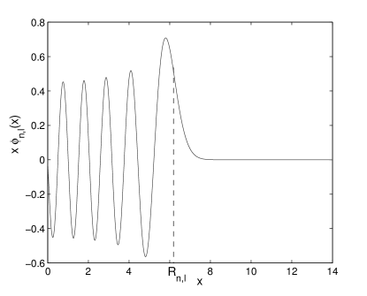
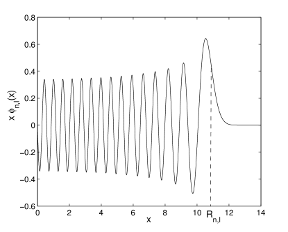
Figure 1: The reduced oscillator state $\varphi_{n,l}(x)$ with a classical turning point $R_{n,l}$ for $l=0$ and two values of $n$: $n=10$ (left) and $n=30$ (right). The function oscillates $n$ times on the interval $[0,R_{n,l}]$. Since $R_{n,l}$ only grows with $\mathcal{O}(\sqrt{n})$ the state becomes rapidly oscillating as $n$ grows.

The Bessel transform $\tilde{F_{l}}(k)$ of a function $F_{l}(x)$ is defined as

$$\tilde{F}_{l}(k):=\sqrt{\frac{2}{\pi}}\int_{0}^{\infty}F_{l}(x)\hat{j}_{l}(kx)dx.$$ (10)

where $\hat{j}_{l}(kx)$ is a Riccati–Bessel function, the regular solution of the radial Schrödinger equation without potential, (2). It is connected with the ordinary Bessel function in a following way $\hat{j}_{l}(x)=\sqrt{\pi x/2}\,J_{l+1/2}(x)$. The Bessel transform of an oscillator state is again an oscillator state

$$\tilde{\varphi}_{n,l}(k)=(-1)^{n}b\,\varphi_{n,l}(kb^{2}),$$ (11)

with a classical turning point $K_{n,l}=R_{n,}/b^{2}=\sqrt{4n+2l+3}/b$. This relation that can easily be derived using e.g. formula (7.421.4) from [35]. The oscillator states therefore form an orthonormal basis of $L^{2}([0,\infty[)$ that diagonalizes the Bessel transform. Similar properties hold for the Cartesian oscillator state based on Hermite polynomials, see, for example, [3].

An other important property that will be used in the remainder of the text is the following:

Proposition 2.1.

Let $\psi_{l}$ a function that behaves as $x^{l}$ in $x=0$. The projection on the oscillator state $\varphi_{n,l}$ can be calculated with either $\psi_{l}$ or its Bessel transform $\tilde{\psi}_{l}$ as:

$$c_{n,l}=\int_{0}^{\infty}\varphi_{n,l}(x)\psi_{l}(x)dx=(-1)^{n}b\int_{0}^{\infty}\varphi_{n,l}(x)\tilde{\psi}_{l}(x)dx.$$ (12)

Proof.

Since Parseval’s theorem holds we can calculate $c_{n}$ either with $\varphi_{n,l}$ or its Bessel transform

$$c_{n,l}=\int_{0}^{\infty}\varphi_{n,l}(x)\psi_{l}(x)dx=\int_{0}^{\infty}\tilde{\varphi}_{n,l}(k)\tilde{\psi}_{l}(k)dk.$$ (13)

But since $\tilde{\varphi}_{n,l}(k)=(-1)^{n}b\varphi_{n,l}(kb^{2})$, the oscillator state in the latter integral is the same as in the first integral, after substitution of variables and up to a constant.∎

This result will be used in the next section to derive the asymptotic formula for $c_{n,l}$ with large $n$. This symmetry between $\psi_{l}(x)$ and its Bessel transform $\tilde{\psi_{l}}(k)$ should also hold in the asymptotic formula.

The kinetic energy operator $T_{i,j}^{l}$ is a tri-diagonal matrix. For the oscillator basis the non-zero elements are

$$T^{l}_{i,j}=\int_{0}^{\infty}\varphi_{i,l}(x)\left(-\frac{1}{2}\frac{d^{2}}{dx^{2}}+\frac{l(l+1)}{2x^{2}}\right)\varphi_{j,l}(x)dx=\left\{\!\!\begin{array}[]{c@{\quad}l}\left(2i+l+\frac{3}{2}\right)\frac{\omega}{2}&\text{for }j=i,\\ -\sqrt{i\,\left(i+l+\frac{1}{2}\right)}\frac{\omega}{2}&\text{for }j=i-1,\\ -\sqrt{(i+1)\left(i+l+\frac{3}{2}\right)}\frac{\omega}{2}&\text{for }j=i+1.\end{array}\right.$$ (14)

For the remainder of the text we will consider only the case of zero angular momentum and drop $l$ from the notation. All results, however, are valid for arbitrary $l$.

2.3 The asymptotic formula

In [36] an asymptotic formula was derived for the projection of a smooth radial function $\psi$ on the state $\varphi_{n}$. The derivation uses stationary phase arguments to exploit the increase of oscillations as $n\rightarrow\infty$. We repeat here the derivation of the results.

There are two main contributions to the value of the integral

$$c_{n}=\int_{0}^{\infty}\varphi_{n}(x)\psi(x)dx\approx I_{0}+I_{R_{n}}.$$ (15)

There is a first contribution, denoted $I_{0}$, of the left integration boundary near zero. There is a second contribution, denoted $I_{R_{n}}$, from the point of stationary phase, which is the classical turning point where the oscillations stop (see Figure 1). Here we provide only general steps of calculating this integral in the asymptotic region. More details can be found in [36].

The contribution from the classical turning point can be calculated by approximating the oscillator state $\varphi_{n}$ near the classical turning point by an Airy function as

$$\varphi_{n}(x)\approx\frac{2}{b}\left(\frac{b^{4}}{2R_{n}}\right)^{1/6}\mathrm{Ai}\left[\left(\frac{2R_{n}}{b}\right)^{1/3}(x-R_{n})\right]\quad\text{if}\quad|x-R_{n}|\ll 1.$$ (16)

The integral representation of this Airy function and the stationary phase approximation leads to the contribution of the turning point to the integral

$$I_{R_{n}}\approx b\sqrt{\frac{2}{R_{n}}}\psi(R_{n}).$$ (17)

The contribution of the left integration boundary, $I_{0}$, can be derived by approximating the oscillator state near the origin by a Riccati–Bessel function

$$\varphi_{n}(x)\approx(-1)^{n}\frac{\sqrt{2}}{b}\sqrt{\frac{2}{\pi K_{n}}}\hat{j}_{0}(K_{n}x),$$ (18)

where $K_{n}$ is the classical turning point of the oscillator state in the momentum space. Then the contribution from the origin becomes

$$I_{0}\approx(-1)^{n}\frac{1}{b}\sqrt{\frac{2}{K_{n}}}\tilde{\psi}(K_{n}).$$ (19)

And the resulting asymptotic approximation of the oscillator coefficients becomes

$$c_{n}\approx(-1)^{n}\frac{1}{b}\sqrt{\frac{2}{K_{n}}}\tilde{\psi}(K_{n})+b\sqrt{\frac{2}{R_{n}}}\psi(R_{n})\quad\text{if}\quad n\gg 1.$$ (20)

This relation has a contribution from the turning points in the coordinate space, $R_{n}$ and the Fourier space, $K_{n}$. Note that it satisfies the symmetry observed in 2.1 above.

Note that Eq. (20) as well as the similar equation in [36] does not provide the order of the approximation. This is one of the shortcomings that will be addressed in the current paper.

2.4 Scattering calculations in the oscillator representation

We now discuss how a finite linear system can be obtained that solves for the wave function in the interaction region and the phase shift, describing the solution in the asymptotic region. The presentation here is based on the asymptotic formula and differs from how the method was derived historically. For more detail about the formulation of the original $J$-matrix method we refer to [9] and [14].

Let $\psi(x)$ be a smooth two-body radial scattering state with a bounded energy, depending on one spatial coordinate (can be always reduced using center-of-mass relative coordinates and spherical coordinates). Since it is a scattering state, the function does not go to zero as $x\rightarrow\infty$. However, its Bessel transform $\tilde{\psi}(k)$ goes to zero as $k\rightarrow\infty$. This means that, as $n$ grows, the only contribution to the expansion coefficient $c_{n}$ comes from the classical turning point in coordinate space. So, for a scattering state $\psi$ with total energy $E=k^{2}/2$ the solution is asymptotically $\hat{j}_{l}(kr)+\tan(\delta_{l})\hat{n}_{l}(kr)$ where $\delta_{l}$ is the phase shift [37] holds that

$$c_{n}\approx b\sqrt{\frac{2}{R_{n}}}\psi(R_{n})=b\sqrt{\frac{2}{R_{n}}}\left(\hat{j}_{l}(kR_{n})+\tan(\delta_{l})\hat{n}_{l}(kR_{n})\right),$$ (21)

where $\hat{j}_{l}$ and $\hat{n}_{l}$ are the regular and irregular solutions of the free-particle equation. The $c_{n}$ becomes the representation of $\psi$ on the grid of classical turning points $R_{n}$.

The aim of a one-dimensional radial scattering calculation is to find a numerical approximation to $\tan(\delta_{l})$ for a given potential $V$. This can be achieved by writing the solution in the oscillator representation as

$$c_{n,l}=\begin{cases}c^{0}_{n,l}+j_{n,l}+\tan(\delta_{l})\,n_{n,l}&n<N\\ j_{n,l}+\tan(\delta_{l})\,n_{n,l}&n\geq N,\end{cases}$$ (22)

where $j_{n,l}$ is the regular solution of the homogeneous three-term recurrence relation

$$T_{n,n-1}j_{n-1,l}+(T_{n,n}-E)j_{n,l}+T_{n,n+1}j_{n+1,l}=0,$$ (23)

where as $n\gg 1$ holds that $j_{n,l}=b\sqrt{2/R_{n}}\,\hat{j}_{l}(kR_{n})$. The $n_{n,l}$ is the irregular solution of the recurrence relation that goes as $n_{n,l}=b\sqrt{2/R_{n}}\,\hat{n}_{l}(kR_{n})$ when $n$ becomes large.

With the form (22) we reduce the infinite linear system to a finite dimensional problem with a set of $N+1$ unknowns $\{c^{0}_{i,l},\tan\delta_{l}\}$. Once solved we simultaneously obtain the wave function of the system, $\{c^{0}_{i,l}\}$, and the scattering information, $\tan(\delta_{l})$.

A detailed description of the construction of this linear system, known as the $J$-matrix, can be found in [14].

2.5 The hybrid $J$-matrix and ECS method

In [33] the asymptotic formula (20) was used to introduce a hybrid oscillator and grid representation for the Schrödinger equation that is useful for scattering calculations where an asymptotic form such as (21) is not explicitly known. Such a situation appears in breakup reactions of three or more particles.

Let $\psi(x)$ be again a smooth one-dimensional radial scattering state with a bounded energy such that

$$c_{n}\approx b\sqrt{\frac{2}{R_{n}}}\psi(R_{n}).$$ (24)

holds. The $c_{n}$ becomes the representation of $\psi$ on the grid of classical turning points $R_{n}$. The grid distance between these points becomes smaller when $n$ increases since

$$h_{n}=R_{n}-R_{n-1}\approx b^{2}\frac{2}{R_{n}}.$$ (25)

However, the asymptotic $\psi$ does not necessarily need to be represented on the grid of turning points $R_{n}$. Another option is, for example, a regular grid of equally spaced points.

The hybrid JM-ECS method represents the one-dimensional radial wave function as a vector ${\sf\Psi}$ in $\mathbb{C}^{N+K}$, where

$${\sf\Psi}=(c_{0},c_{1},\ldots,c_{N-1},\psi(R_{N}),\psi(R_{N}\!+\!h),\ldots,\psi(R_{N}\!+\!(K\!-\!1)h)).$$ (26)

The first $N$ elements represent the wave function in the oscillator representation. While the remaining $K$ elements represent $\psi$ on an equidistant grid that starts at $R_{N}$, the $N$-th classical turning point, and runs up to $R_{N}+(K-1)h$ with a grid distance $h$ equal to the difference of the last two turning points of the oscillator representation $h=R_{N}-R_{N-1}$. It is assumed that the matching point that connects the oscillator to finite–difference representation corresponds to a large index $N$ such that the asymptotic formula, (24), applies.

Again, the kinetic energy operator in this hybrid representation is tridiagonal since in both finite–difference and oscillator representations it is tridiagonal. One should only be careful in matching both representations. To obtain the kinetic energy in the last point of the oscillator representation, the tridiagonal kinetic energy formula (14) is used. It involves a recurrence relation connecting the three terms $c_{N-2}$, $c_{N-1}$ and $c_{N}$. The latter, the coefficient $c_{N}$, is unknown. Only $\psi(R_{N})$ is available on the grid. Using the asymptotic relation (24), however, it is possible to calculate the required matrix element as follows:

$$\begin{split}(Tc)_{N-1}=T_{N-1,N-2}c_{N-2}+T_{N-1,N-1}c_{N-1}+T_{N-1,N}b\sqrt{2/R_{N}}\psi_{l}(R_{N}).\end{split}$$

To calculate the kinetic energy in the first point of the finite difference grid, the second derivative of the wave function has to be known. To approximate the latter with a finite difference formula, one needs the wave function in the grid points $R_{N-1}$, $R_{N}$ and $R_{N}+h$. Again it is possible to apply (24) to obtain $\psi(R_{N-1})$ in terms of $c_{N-1}$:

$$\psi^{\prime\prime}(R_{N})\approx\frac{c_{N-1}/(b\sqrt{2/R_{N-1}})-2\psi(R_{N})+\psi(R_{N}+h)}{h^{2}}.$$

The coupling between both representations around the matching point is sketched in Figure 2, together with the terms involved to determine the correct matching.

Oscillator           Finite Differences

$$\overbrace{\vphantom{\rule[5.0pt]{5.0pt}{5.0pt}}c_{n-2}\;\;\quad c_{N-1}\qquad\psi(R_{N})}^{Tc_{N-1}}\quad\psi(R_{N}+h)\makebox[0.0pt][r]{$\underbrace{\phantom{c_{N-1}\qquad\psi(R_{N})\quad\psi(R_{N+1})\vphantom{\rule[-20.0pt]{20.0pt}{20.0pt}}}}_{\psi^{\prime\prime}(R_{N})}$}$$

Figure 2: Illustration on the calculation of the kinetic energy matrix elements that are calculated in the last point $R_{N-1}$ of the oscillator representation and in the first point $R_{N}$ of the finite difference representation. To calculate $T$ applied to a solution vector we need to translate the oscillator representation to the grid. Vice versa for the application of the finite difference stencil approximation to the second derivative.

However, in the next section we will show that the asymptotic matching condition that is used in [33] to couple both representations, is only accurate to $\mathcal{O}(R_{N}^{-1})$, while the outer grid is accurate to order $\mathcal{O}(h^{2})=\mathcal{O}(R_{N}^{-2})$. Therefore the largest error is made in the matching condition that couples both representations.

Note that introducing an absorbing layer is easy once the oscillator representation is coupled to a grid representation. For example ECS is implemented by extending the grid with a complex scaled part [24].

3 Higher–order asymptotic formula

In this section we derive a higher–order asymptotic formula. It not only takes into account the function values in the turning point $R_{n}$ but also the third derivative in this point. A similar asymptotic formula was derived by S. Igashov in [34], however, it did not include the contributions from the Fourier space.

Proposition 3.1.

Let $\psi(x)$ be a regular scattering state that behaves as $x^{l}$ in $x=0$, that is infinitely differentiable and $\varphi_{n}(x)$ is a reduced oscillator state, solution of (9). Then the projection of the scattering state on the oscillator state can be approximated as

$$c_{n}=\int_{0}^{\infty}\,\varphi_{n}(x)\,\psi(x)dx=b\sqrt{\frac{2}{R_{n}}}\left(\psi(R_{n})+\frac{b^{4}}{6R_{n}}\psi^{\prime\prime\prime}(R_{n})\right)+\mathcal{O}(R_{n}^{-5/2}).$$ (27)

This expresses the expansion coefficient in terms of the wave function and its derivatives in the classical turning point $R_{n}$.

Proof.

The oscillator Eq. (9) can be rewritten as

$$\left[-\frac{d^{2}}{dx^{2}}+\frac{2R_{n}(x-R_{n})}{b^{4}}+\frac{(x-R_{n})^{2}}{b^{4}}\right]\varphi_{n}(x)=0.$$ (28)

For $R_{n}\gg|x-R_{n}|$ (which means either $n\gg 1$ or $|x-R_{n}|\approx 0$), we can neglect the quadratic term in this equation and get the Airy equation with the solution

$$\varphi_{n}(x)\approx\varphi_{n}^{(0)}(x)=\frac{2}{b}\left(\frac{b^{4}}{2R_{n}}\right)^{1/6}\mathrm{Ai}\left[\left(\frac{2R_{n}}{b^{4}}\right)^{1/3}(x-R_{n})\right],$$ (29)

where the normalization is chosen such that it coincides with the oscillator state near the classical turning point $R_{n}$.

This can be further improved by writing $\varphi_{n}(x)=\left(1+u_{n}(x)\right)\varphi^{(0)}_{n}$ and inserting this in the oscillator equation. The equation for $u_{n}(x)$ becomes

$$-\frac{1}{2}u_{n}^{\prime\prime}\varphi_{n}^{(0)}-u_{n}^{\prime}{\varphi_{n}^{(0)}}^{\prime}-\frac{1}{2}u_{n}\,{\varphi_{n}^{(0)}}^{\prime\prime}+\left(R_{n}(x-R_{n})+\frac{1}{2}(x-R_{n})^{2}\right)u_{n}\varphi_{n}^{(0)}=-\frac{1}{2}(x-R_{n})^{2}\varphi_{n}^{(0)}.$$ (30)

Using that

$${\varphi_{n}^{(0)}}^{\prime}=\left(2R_{n}/b^{4}\right)^{1/3}\mathrm{Ai}^{\prime}\left[\left(2R_{n}/b^{4}\right)^{1/3}(x-R_{n})\right]$$

and

$${\varphi_{n}^{(0)}}^{\prime\prime}=\left(2R_{n}/b^{4}\right)^{2/3}\mathrm{Ai}^{\prime\prime}\left[\left(2R_{n}/b^{4}\right)^{1/3}(x-R_{n})\right]$$

the equation (30) becomes

$$-\frac{1}{2}u_{n}^{\prime\prime}\varphi_{n}^{(0)}-u^{\prime}\left(\frac{2R_{n}}{b^{4}}\right)^{1/3}\mathrm{Ai}^{\prime}\left[\left(\frac{2R_{n}}{b^{4}}\right)^{1/3}(x-R_{n})\right]$$

$$-\frac{1}{2}u_{n}\,\left(\frac{2R_{n}}{b^{4}}\right)^{2/3}\mathrm{Ai}^{\prime\prime}\left[\left(\frac{2R_{n}}{b^{4}}\right)^{1/3}(x-R_{n})\right]+\left(R_{n}(x-R_{n})+\frac{1}{2}(x-R_{n})^{2}\right)u_{n}\,\varphi_{n}^{(0)}=-\frac{1}{2}(x-R_{n})^{2}\varphi_{n}^{(0)}.$$ (31)

In the limit $n\rightarrow\infty$, the term with $R_{n}(x-R_{n})$ dominates compared to $(1/2)(x-R_{n})^{2}$ and the other terms since both the first and second derivative of $\mathrm{Ai}(x)$ around zero are bounded. We find that $u_{n}(x)\approx-(x-R_{n})/(2R_{n})$ is a solution of the remaining equation.

At this time we will not consider the contributions to the integral for the boundary at zero. This contribution will be equal to the contribution from the Fourier space as in Eq. (20) and for scattering states and large $n$ this contribution is negligible. So we can lower the integration boundary and write

$$c_{n}\approx\frac{2\sqrt{a_{n}}}{b}\int_{-\infty}^{\infty}\psi(x+R_{n})\mathrm{Ai}(x/a_{n})\left(1-\frac{x}{2R_{n}}\right)dx,$$ (32)

where $a_{n}:=(b^{4}/2R_{n})^{1/3}$ and we have substituted the integration variable $x\rightarrow x+R_{n}$.

The value of this integral will be determined by the behavior around $R_{n}$, the point of stationary phase. Since the function $\psi$ is infinitely differentiable we can Taylor expand

$$c_{n}\approx\frac{2\sqrt{a_{n}}}{b}\int_{-\infty}^{\infty}\sum_{m=0}^{\infty}\frac{x^{m}}{m!}\psi^{(m)}(R_{n})\left(1-\frac{x}{2R_{n}}\right)\mathrm{Ai}(x/a_{n})dx$$ (33)

All integrals in these series can be calculated explicitly using specific properties of Airy function (see page 52 of [38]).

$$\int_{-\infty}^{\infty}\mathrm{Ai}(x)x^{3k}dx=\frac{(3k)!}{3^{k}k!}\quad\text{and}\quad\int_{-\infty}^{\infty}\mathrm{Ai}(x)x^{3k+1}dx=\int_{-\infty}^{\infty}\mathrm{Ai}(x)x^{3k+2}dx=0.$$ (34)

We finally get

$$\begin{split}c_{n}&\approx\frac{2a_{n}^{3/2}}{b}\sum_{k=0}^{\infty}\frac{a_{n}^{3k}}{3^{k}k!}\left(\psi^{(3k)}(R_{n})-\frac{a_{n}^{3}}{2R_{n}}\psi^{(3k+2)}(R_{n})\right)\\ &=b\sqrt{\frac{2}{R_{n}}}\sum_{k=0}^{\infty}\frac{1}{k!}\left(\frac{b^{4}}{6R_{n}}\right)^{k}\left(\psi^{(3k)}(R_{n})-\frac{b^{4}}{4R_{n}^{2}}\psi^{(3k+2)}(R_{n})\right).\end{split}$$ (35)

In lowest order (in terms of $1/R_{n}$) this gives us exactly the initial relation (24). Including the next order correction we get a relation (27). For testing purposes we also include terms of the next order $1/R_{n}^{2}$

$$\begin{split}c_{n}&=b\sqrt{\frac{2}{R_{n}}}\left(\psi(R_{n})+\frac{b^{4}}{6R_{n}}\psi^{\prime\prime\prime}(R_{n})\right.\left.+\frac{1}{R_{n}^{2}}\left(\frac{b^{8}}{72}\psi^{(6)}(R_{n})-\frac{b^{4}}{4}\psi^{\prime\prime}(R_{n})\right)+\mathcal{O}(\frac{1}{R_{n}^{3}})\right)\end{split}$$ (36)

∎

Note that a similar result is readily obtained for Cartesian harmonic oscillator states that are based on the Hermite polynomials. There, however, there is a contribution from both turning points, one from $R_{n}=\sqrt{2n+1}$ and $R_{n}=-\sqrt{2n+1}$.

Corollary 3.2.

Let $\psi(x)$ be a function that behaves as $x^{l}$ in $x=0$ that is infinitely differentiable, then the asymptotic expansion coefficient is

$$c_{n}= \int_{0}^{\infty}\,\varphi_{n}(x)\,\psi(x)dx=b\sqrt{\frac{2}{R_{n}}}\left(\psi(R_{n})+\frac{b^{4}}{6R_{n}}\psi^{\prime\prime\prime}(R_{n})\right)$$

$$+\frac{(-1)^{n}}{b}\sqrt{\frac{2}{K_{n}}}\left(\tilde{\psi}(K_{n})+\frac{1}{6b^{4}K_{n}}{\tilde{\psi}}^{\prime\prime\prime}(K_{n})\right)+\mathcal{O}(n^{-5/4}).$$ (37)

Proof.

The asymptotic formula should have the same result when we interchange $\psi(x)$ with its Bessel transform $\tilde{\psi}(k)$ as a result of Proposition 2.1. Indeed, the integral

$$c_{n}=(-1)^{n}b\int_{0}^{\infty}\varphi_{n}(k)\tilde{\psi}(k)dk$$

will have a contribution from integral boundary near 0 and a contribution from the turning point $K_{n}$ in Fourier space. The latter is, with the help of the previous results, $(-1)^{n}b\sqrt{2/K_{n}}(\tilde{\psi}(K_{n})+\tilde{\psi}^{\prime\prime\prime}(K_{n})/6b^{4}K_{n})$. While the contribution from boundary become the contribution from the turning point $R_{n}$ in coordinate space.

∎

Example 3.3.

We illustrate the convergence of the asymptotic formula (37) with an application to the function $\psi(x)=\exp(-ax)\sin(x)$. We give results for two choices of $a$. As the scale of the representation is defined by the oscillator length $b$, the result will change with its choice. If the product $ab$ is large, the Fourier components will dominate in the expansion coefficient. When $ab$ is small the function $\psi$ resembles a scattering state, on a scale defined by $b$, and the coordinate approximation will dominate. However, as Figure 3 illustrates the combined formula always gives the correct result. We see an overall convergence with $n^{-5/4}$. This is smaller than $\mathcal{O}(h_{n}^{2})$ which goes as $\mathcal{O}(1/n)$. In general, it is possible to construct a function, for which both coordinate and Fourier terms fail to represent the exact oscillator coefficient, but the combined formula remains valid even in this case (see Figure 4).

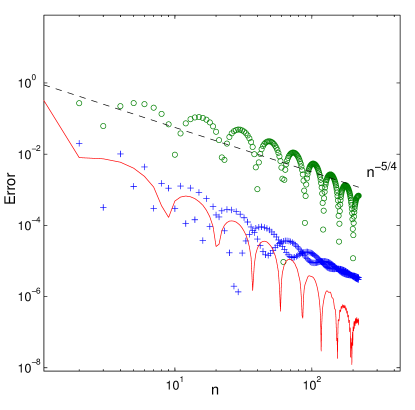
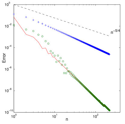
Figure 3: Convergence of the general asymptotic formula (37) with only coordinate terms (crosses), only Fourier terms (circles), both coordinate and Fourier terms (solid line) for test function $\psi(x)=\exp(-ax)\sin(x)$ with different values of $a$: left figure — $a=0.2$, right figure — $a=1.5$ ($b=1$ in both cases)

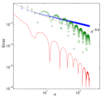
Figure 4: Convergence of the general asymptotic formula (37) for the test function $\psi(x)=\exp(-ax)\cos(x)$ with $a=0.2$, for which neither coordinate (crosses) nor Fourier terms (circles) give accurate result, while the combined formula (solid line) does.

Example 3.4.

We have verified the asymptotic relations derived in the previous section with a numerical experiment using the wave function $\psi(x)=\sin(kx)$. We calculate oscillator coefficients directly and compare them against the values obtained with asymptotic formulas of different order derived previously (see Fig. 5).

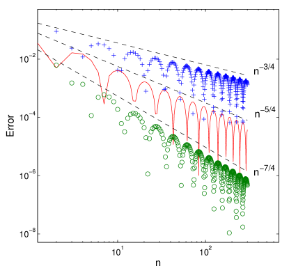
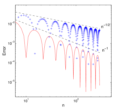
Figure 5: Convergence of the asymptotic formula (36) (left) and the inverse asymptotic formula (41) (right) with different number of terms included (crosses — one term, solid line — two terms, circles — three terms). The test function has the form $\psi(x)=\sin(kx)$ with $k=1.5$ and the oscillator length $b=0.8$

3.1 Inverse relation

The asymptotic expansion coefficient is an approximation with the help of the functions values of $\psi$ evaluated at certain grid points. It is also useful to derive in inverse relation that allows us to construct the function value in certain grid points given the expansion coefficients.

To approximate $c_{n}$ with Eq. (27) the function value and its third derivative need to be calculated at the turning point $R_{n}$. When only the function values of $\psi$ are available at the turning points $R_{n}$, the third derivative can be approximated by finite differences.

The coefficient is then calculated as

$$c_{n}=b\sqrt{\frac{2}{R_{n}}}\left(\psi(R_{n})+\frac{b^{4}}{6R_{n}}\sum_{k}D^{(3)}_{k}\psi(R_{n+k})\right)+\mathcal{O}(R_{n}^{-5/2})+R_{n}^{-3/2}\epsilon_{n},$$ (38)

where $D^{(3)}$ is the matrix with coefficients that approximates the third derivative and $k$ indicates the stencil points and $\epsilon_{n}$ is the error term of this approximation. In case of 5-point finite difference approximation $k\in\{-2,-1,0,1,2\}$. Note that the grid of turning points $R_{n}$ is an irregular grid and the coefficients will depend on the local distances between the neighboring grid points. The error of the approximation $\epsilon_{n}$ will also depend on the local grid distances as $\mathcal{O}(h^{p})\sim\mathcal{O}(R_{n}^{-p})$, where $p$ is the order of the approximation.

The resulting transformation can be represented by a banded sparse matrix $U$

$$c_{n}=\sum_{k}U_{nk}\psi(R_{k})+\mathcal{O}(R_{n}^{-5/2}).$$ (39)

Note that the matrix elements of $U$ will only depend on the values of $R_{n}$. Indeed, The differential operator $D^{(3)}$ only depends on the grid distances and so do the coefficients of the asymptotic expression.

The relation (38) translates $\psi$ on the grid of turning points to corresponding $c_{n}$. It is also useful to derive the inverse relation that gets $\psi(R_{n})$ from known values of $c_{n}$. We can not use a direct inversion of Eq. (27) since it involves the third derivative, a dense operator in the oscillator representation. However, an approximate inverse relation can be obtained by rearranging terms in (38) as

$$\psi(R_{n})=\frac{1}{b}\sqrt{\frac{R_{n}}{2}}c_{n}-\frac{b^{4}}{6R_{n}}\sum_{k}D^{(3)}_{k}\psi(R_{n+k})+\mathcal{O}(R_{n}^{-2})+R_{n}^{-1}\epsilon_{n}$$ (40)

and replacing values of the wave function in the right–hand side by oscillator coefficients using only the first term of (24), i.e. $\psi(R_{n})=(1/b)\sqrt{R_{n}/2}\,c_{n}+\mathcal{O}(R_{n}^{-1})$. This only introduces an error of the order of $\mathcal{O}(R_{n}^{-1})$ but combined with the $1/R_{n}$ this gives the approximate inverse relation

$$\psi(R_{n})=\frac{1}{b}\sqrt{\frac{R_{n}}{2}}c_{n}-\frac{b^{3}}{6R_{n}}\sum_{k}D^{(3)}_{k}\sqrt{\frac{R_{n+k}}{2}}c_{n+k}+\mathcal{O}(R_{n}^{-2})$$ (41)

that is accurate to $\mathcal{O}(R_{n}^{-2})$. An example of the resulting numerical accuracy of this inverse asymptotic relation is shown on the right panel of figure 5. Also this transformation can be presented as a sparse banded matrix multiplication

$$\psi(R_{n})=\sum_{n}W_{nk}c_{k}+\mathcal{O}(R_{n}^{-2}).$$ (42)

Again the matrix elements of $W$ only depend on the values of the turning points $R_{n}$.

Combining the two relations leads to an approximate partition of unity:

$$UW=I+\mathcal{O}(R_{n}^{-2}).$$ (43)

It is important to note that since these transformation matrices only depend on values of $R_{n}$ they can, in principle, both be defined for an arbitrary grid.

3.2 Approximate discretization of Operators

With the help of these two transformation matrices $U$ and $W$ we can now build an approximate oscillator representation of an operator $Q$ using its finite difference representation. Let $Q^{(fd)}$ be the finite difference representation of $Q$ on the grid $R_{n}$. Then the application of the $Q$ on $\psi$ can be written as

$$(Q\psi)^{(osc)}_{n}=\sum_{m}Q^{(osc)}_{nm}c_{m}=\sum_{m}\check{Q}^{(osc)}_{nm}c_{m}+\mathcal{O}(n^{-1}),\qquad\text{where}\quad\check{Q}^{(osc)}_{nm}:=[UQ^{(fd)}W]_{nm}.$$

We illustrate the accuracy of this relation on a second derivative operator $D^{(}2)$, as we intend to apply the constructed representation to Helmholtz-type equations.

$$\check{D}^{(2)(osc)}=UD^{(2)(fd)}W,$$ (44)

where $D^{(2)(fd)}$ is a finite difference matrix of the second derivative. To analyze the accuracy of this approximation Figure 6 shows the result of the error operator defined as $(D^{(osc)}-\check{D}^{(osc)})$ acting on the vector of oscillator coefficients of the test function $\psi(x)=\sin(kx)$. For comparison we show the error of the approximate identity operator, that can be defined as $(I-\check{I})=(I-UW)$. We see that both considered error operators decay as $\mathcal{O}(n^{-1})$ in high-$n$ region. This means that our approximate operators are asymptotically equal to the exact ones and we can expect the same order of convergence in a solution of the scattering problem.

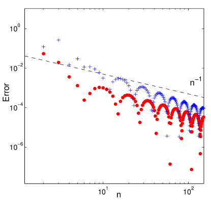
Figure 6: Convergence of the approximate second derivative operator $\check{D}=UD^{(fd)}W$ (crosses) and the approximate identity operator $\check{I}=UW$ (circles) with a test function of the form $\psi(x)=\sin(kx)$ ($k$ and $b$ are the same as in Figure 5)

It is important to note that all matrices in (44) can be built for any arbitrary spatial grid, though it will not be an approximate oscillator representation. But we can modify this grid only in the asymptotic region (e.g. to implement the absorbing boundary with ECS). Then the coefficients $c_{n}$ have no physical meaning as oscillator coefficients but the coordinate wave function can sill be reconstructed with (42).

4 High-order hybrid representation for scattering problems

The aim is now to build a hybrid representation for scattering calculations where the oscillator basis is used in the internal region and finite differences in the outer region. The matching of the two should use the higher–order asymptotic formula (27). However, the strategy displayed on Fig. 2 cannot be easily applied since the third derivative of the wave function needs to be estimated from several neighboring points symmetrically distributed on both sides of the matching point. But in the matching point we only have the required function values on one side of the matching point. This arguments holds both for the oscillator and for the finite difference representation. We therefore present a matching strategy that differs from the proposal of [33].

Consider a arbitrary grid $\bar{R}_{n}$ in $[0,\infty]$ with $n=1,2,\ldots$ that differs from the grid of turning points $R_{n}$. On this grid we can construct the differential operator $D^{(3)}$ and construct the operators $\bar{U}$ and $\bar{W}$ by replacing every appearance of $R_{n}$ in equations (38) and (41) by $\bar{R}_{n}$. Similarly, for a function $\psi$ sampled in the grid points $\bar{R}_{n}$ we can calculate

$$\bar{c}_{n}=\sum_{k}\bar{U}_{nk}\psi(\bar{R}_{k}).$$ (45)

These coefficients $\bar{c}_{n}$ are not the expansion coefficients of the function $\psi$ in the oscillator function basis. Only when $\bar{R}_{n}$ equals $R_{n}$, the oscillator turning points, then the $\bar{c}_{n}$ are approximations to the oscillator expansion coefficients $c_{n}$.

To build the hybrid representation, we choose the grid $\bar{R}_{n}$ such that first $N+1$ points correspond to the turning points $R_{n}$. The remaining points of $\bar{R}_{n}$, for $n>N+1$, are chosen to correspond to points on a equidistant finite difference grid. To solve a scattering problem the equation (2) needs to be discretized with finite differences on the grid $\bar{R}_{n}$ and then transformed with the help of $\bar{U}$ and $\bar{W}$ into

$$\sum_{j}\left(\bar{U}H^{fd}\bar{W}-E\bar{U}\bar{W}\right)_{ij}\bar{c}_{j}=(\bar{U}f)_{i}$$ (46)

to arrive at an equation for $\bar{c}_{i}$.

The first $N$ coefficients of $\bar{c}_{n}$ correspond now to approximations to oscillator expansion coefficients $c_{n}$. However, because $n$ is low, they are only a poor approximation. The idea is now to replace the first $N$ coefficients with the exact coefficients. At the same time we replace the first $N$ rows of the matrix with the exact operator in the oscillator representation. The linear system then becomes

$$\left(\begin{array}[]{ccc|cc}H^{(osc)}_{00}-E&\ldots&H^{(osc)}_{0N}&H^{(osc)}_{0N+1}&\ldots\\ H^{(osc)}_{10}&\ldots&H^{(osc)}_{1N}&H^{(osc)}_{1N+1}&\ldots\\ \vdots&&\vdots&\vdots&\\ H^{(osc)}_{N0}&\ldots&H^{(osc)}_{NN}-E&H^{(osc)}_{NN+1}&\ldots\\ \hline\cr[\bar{U}H^{(fd)}\bar{W}]_{N+1,0}&\ldots&[\bar{U}H^{(fd)}\bar{W}]_{N+1,N}&[\bar{U}(H^{(fd)}-E)\bar{W}]_{N+1,N+1}&\ldots\\ \vdots&&\vdots&\vdots&\end{array}\right)\left(\begin{array}[]{c}\vphantom{H^{(N)}_{N}}c_{0}\\ \vphantom{H^{(N)}_{N}}c_{1}\\ \vdots\\ \vphantom{H^{(N)}_{N}}c_{N}\\ \hline\cr\vphantom{H^{(N)}_{N}}\bar{c}_{N+1}\\ \vdots\end{array}\right)=\left(\begin{array}[]{c}f^{(osc)}_{0}\\ f^{(osc)}_{1}\\ \vdots\\ f^{(osc)}_{N}\\ \hline\cr\sum_{j}\bar{U}_{N+1j}f(x_{j})\\ \vdots\end{array}\right),$$ (47)

where $H^{(osc)}$ is the representation of the Hamiltonian in the oscillator representation and $H^{(fd)}$ in the finite difference representation.

We emphasize the difference with [33]. Here we do not match two regions by using the asymptotic formula in one point. Now the representation in the asymptotic region is a fairly good approximation of the oscillator representation. Therefore the structure of the discretized wave function is simpler than (26). Now we have

$$\bar{\sf\Psi}=\left(c_{0},\ldots c_{N},\bar{c}_{N+1},\ldots\bar{c}_{K}\right),$$

where in the initial version of hybrid method, the latter elements of the vector are the function values of $\psi$ in the grid points. Now the internal region is covered by an exact oscillator representation, and the asymptotic region is covered by approximate representation which is based on finite differences and includes the ECS transformation.

4.1 Numerical Illustration

We illustrate the method for a one-dimensional radial example. After the solution of (47), we first reconstruct the coordinate wave function using (42). Outside the range of the potential $V$ the solution can be written as a linear combination $\psi_{sc}=A\hat{h}_{l}^{+}(kx)+B\hat{h}_{l}^{-}(kx)$, where $\hat{h}_{l}^{\pm}$ are the in- and outgoing Riccati-Hankel functions. The coefficient $A$ is then extracted with

$$A=W\left(\psi_{\text{sc}}(x),\hat{h}_{l}^{-}(kx)\right)/W\left(\hat{h}_{l}^{+}(kx),\hat{h}_{l}^{-}(kx)\right),$$ (48)

where $x$ is outside the range of the potential but still on the real part of the ECS domain. The Wronskian is calculated as $W(u,v)=u^{\prime}v-v^{\prime}u$, where the derivatives can be implemented with finite differences. From the Wronskians for $A$ and $B$ we can extract the phase shift of the solution.

It is important to note that the accuracy of the method does not directly depend on the size of the asymptotic region as long as this region is located outside the range of the potential ($V=0$ in the considered part of $\check{H}^{(osc)}$). In this region we use a grid of 150 equidistant points and then the ECS layer that spans 10 dimensionless length units and applies a complex rotation of $45^{\circ}$ to the coordinate axis.

We first consider a model problem with a attractive potential in Gaussian form, $V(x)=-\exp(-x^{2})$, and we limit our consideration to the case of zero total angular momentum $l=0$. Nevertheless, all the conclusions are applicable to higher angular momenta as well. The right panel of Figure 7 shows the error in the scattering phase shift of the considered problem calculated with the original JM-ECS and the new approach. To obtain the reference phase shift we use the highly accurate variable phase approach (VPA). We see that for all energies the new method gives much more accurate and less oscillatory results. The convergence as a function of the number of oscillator states in the inner region of both methods is shown on Figure 8. We see that we arrived at the desired the convergence rate to $N^{-1}$ in both low-energy and high-energy regions.

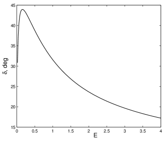
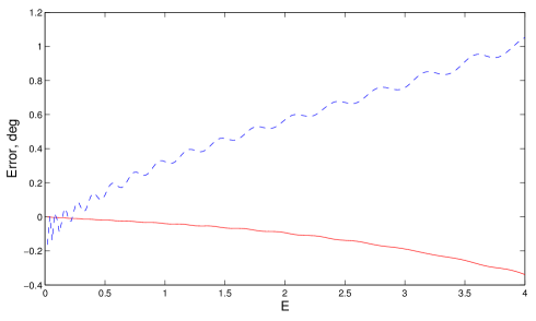
Figure 7: Scattering phase shift of the model problem of Section 4 with a Gaussian potential (left) and the absolute error of the scattering phase shift calculated with JM-ECS (dashed line) and our new approach (solid line) depending on the energy of the system (right). Both calculations were made with 100 functions in the oscillator basis with the oscillator length $b=0.7$.

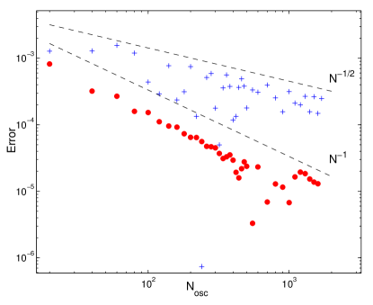
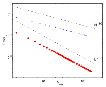
Figure 8: Accuracy of the scattering phase shift calculated with JM-ECS (crosses) and the new method (circles) depending on the size of the oscillator basis. Calculations were made for two values of energy: $E=0.2$, where $\delta=43.73^{\circ}$ (left) and $E=3$, where $\delta=19.67^{\circ}$ (right)

The Gaussian shape of the interaction potential was chosen as the main model problem as it is particularly well adapted to the harmonic oscillator basis and $J$-matrix method for this potential converges for any oscillator length $b$. However we can also test our approach against other short-range potentials. But if the asymptotic behavior of the potential is not Gaussian then the results will converge only for specific values of the oscillator length, that match the range of the potential. Also, if the potential has a special point in the origin (like Yukawa potential) then the convergence will be much slower due to the importance of the Fourier contribution in the potential matrix elements. For additional convergence tests we have chosen two potentials with non Gaussian asymptotics and different behavior in the origin: Morse potential $V(x)=\exp(-2|x/b|)-\exp(-|x/b|)$ and Yukawa potential $V(x)=-\exp(-|x/b|)/x$. In both potentials the potential range is chosen to match the oscillator length of the basis. Figure 9 shows the convergence of the phase shift for these two potentials. We see that in high-energy region the convergence pattern is mostly similar for all potentials as the kinetic energy is much higher than the potential energy in this case. The behavior of the error is much less clear for low energies. The convergence rate appears to be the same here for both methods with Morse potential, for Yukawa potential the convergence rate is blurred due to high oscillations which clearly indicates the importance of Fourier terms. Though we can generally conclude that the new approach always gives better and generally less oscillatory result.

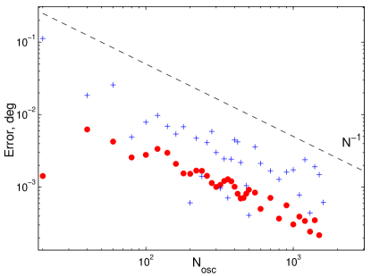
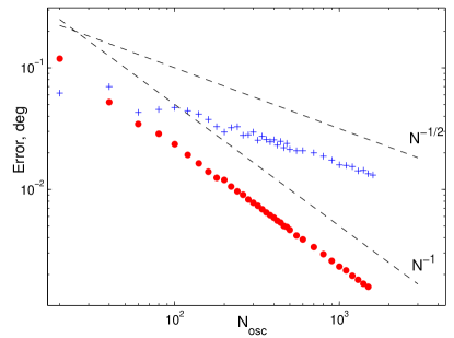
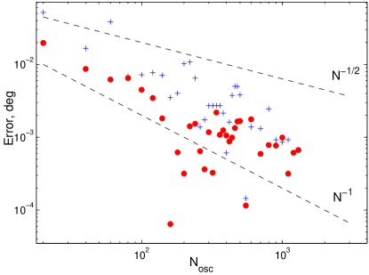
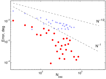
Figure 9: Same as Figure 8 but for the Morse potential (two upper panels) and Yukawa potential (two lower panels)

5 Extension to systems with more particles

The results of the previous sections can be generalized to systems of three and more particles. Let $\mathbf{r}_{1}$ and $\mathbf{r}_{2}$ be two relative coordinates describing a three–body problem. The 6D wave function can be expanded in partial waves

$$\Psi(\mathbf{r}_{1},\mathbf{r}_{2})=\Psi(\rho_{1},\rho_{2},\theta_{1},\theta_{2},\phi_{1},\phi_{2})=\sum_{l_{1},m_{1},l_{2},m_{2}}\frac{\psi_{l_{1},l_{2},m_{1},m_{2}}(\rho_{1},\rho_{2})}{\rho_{1}\rho_{2}}Y_{l_{o}1,m_{1}}(\theta_{1},\phi_{1})Y_{l_{2},m_{2}}(\theta_{2},\phi_{2}).$$ (49)

Such an expansion is used for example to describe double ionization processes in atomic physics [39]

Let $\psi(x,y)$ now be an infinitely differentiable two–dimensional radial scattering wave function that is expanded in the bi-oscillator basis as

$$\psi(x,y)=\sum_{n=0}^{\infty}\sum_{m=0}^{\infty}c_{nm}\varphi_{n}(x)\varphi_{m}(y),$$ (50)

where $x$ and $y$ should be interpreted as two radial coordinates. The expansion coefficient is then calculated as a double integral that can be approximated by applying the asymptotic relation twice. First in the $x$-direction and then in the $y$-direction

$$c_{nm}= \int_{0}^{\infty}\int_{0}^{\infty}\varphi_{n}(x)\varphi_{m}(y)\psi(x,y)\,dxdy$$ (51)

$$= \int_{0}^{\infty}\varphi_{n}(x)\left[\sqrt{2}\,R_{m}^{-1/2}\psi(x,R_{m})+(b^{4}/6)R_{m}^{-3/2}\partial_{yyy}\psi(x,R_{m})+\mathcal{O}(R_{m}^{-5/2})\right]dx$$

$$= 2\,(R_{m}R_{n})^{-1/2}\psi(R_{n},R_{m})+\frac{b^{4}\sqrt{2}}{6}R_{n}^{-3/2}R_{m}^{-1/2}\partial_{xxx}\psi(R_{n},R_{m})+\frac{b^{4}\sqrt{2}}{6}R_{n}^{-1/2}R_{m}^{-3/2}\psi_{yyy}(R_{n},R_{m})$$

$$+\frac{b^{8}}{36}R_{n}^{-3/2}R_{m}^{-3/2}\partial_{xxx,yyy}\psi(R_{n},R_{m})+\mathcal{O}(R_{n}^{-1/2}R_{m}^{-5/2})+\mathcal{O}(R_{m}^{-1/2}R_{n}^{-5/2}).$$

It is important to note that the accuracy depends on both indices $n$ and $m$. For example, when the low order approximation is used for both integrals, there will be error terms of the order $R_{m}^{-1/2}R_{n}^{3/2}$ and $R_{n}^{-1/2}R_{m}^{3/2}$. Along the diagonal, i.e. when $R_{m}=R_{n}$, it is accurate up to order $R_{n}^{-1/2}R_{m}^{-3/2}=R_{n}^{-2}=\mathcal{O}(n^{-1})$, which is of the order $h_{n}^{2}$, with $h_{n}$ the distance between the classical turning points. For the higher–order approximation the error term along the diagonal, where $R_{n}=R_{m}$, will be $R_{n}^{-3}=\mathcal{O}(n^{-3/2})$. In the left panel of Figure 10 we compare the exact expansion coefficients with the first order and second order approximation along the diagonal for $n=m$. The results show an improvement with the higher–order expression over the first order approximation.

However, when one of the indices remains small, for example $m$, then the error becomes asymptotically $\mathcal{O}(R_{n}^{-1/2})$, as expected from (51). As $n$ becomes large, all error terms with a higher–order accuracy decay until the term $O(R_{n}^{-1/2}R_{m}^{-5/2})$ dominates for the higher–order formula, or $O(R_{n}^{-1/2}R_{m}^{-3/2})$ for the low order accuracy. This is shown in the right panel of Figure 10.

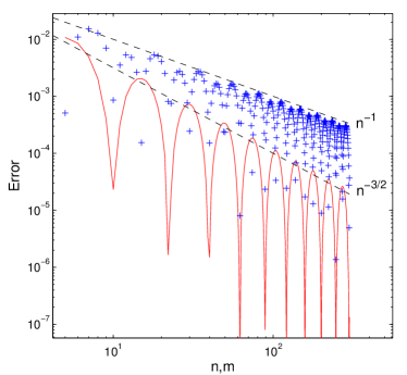
Figure 10: Convergence of the asymptotic formula for two-dimensional radial functions. The error is calculated by comparing the exact expansion coefficient with the asymptotic approximations. The function $f(x,y)=\sin(kx)\sin(ky)$ along the diagonal (n=m, left) and along the line with fixed m=20 (right). Crosses show the first order and solid lines correspond to the second order asymptotic expansion coefficient ($k=1$, $b=1$).

5.1 Three–body scattering problems

In a similar way as in the previous sections we can use the asymptotic formulate to build a hybrid representation that can solve the radial equation of two radial variables that arises after an expansion of a full three–body scattering problem equation in spherical harmonics (49). This typically leads to a set of coupled two–dimensional radial partial waves. A diagonal block of this coupled set reads

$$\left(-\frac{1}{2}\frac{d^{2}}{dx^{2}}-\frac{1}{2}\frac{d^{2}}{dy^{2}}+\frac{l_{1}(l_{1}+1)}{2x^{2}}+\frac{l_{2}(l_{2}+1)}{2y^{2}}+V(x,y)-E\right)\psi(x,y)=\chi(x,y)$$ (52)

with boundary conditions $\psi(x,0)=\psi(0,y)=0$.

The solution of this equation can be represented in a bi-oscillator basis, (50), using two indices $n$ and $m$. Then similar to the two–body case we use approximate oscillator coefficients in the asymptotic region. But there are now three asymptotic regions: first, the region where $n$ is large, second, the region where $m$ is large and finally, the region where both $n$ and $m$ are large. For each of these regions we define approximate oscillator coefficients that take the form:

$$c_{nm}\approx\grave{c}_{nm}:= \sum_{i}U_{ni}\int_{0}^{\infty}\varphi_{m}(y)\psi(R_{i},y)\,dy+\mathcal{O}(R_{n}^{-5/2})\quad\text{where}\quad n\gg 1$$ (53)

$$c_{nm}\approx\acute{c}_{nm}:= \sum_{i}U_{mi}\int_{0}^{\infty}\varphi_{n}(x)\psi(x,R_{i})\,dx+\mathcal{O}(R_{m}^{-5/2})\quad\text{where}\quad m\gg 1$$ (54)

$$c_{nm}\approx\check{c}_{nm}:= \sum_{i,j}U_{ni}U_{mj}\psi(R_{i},R_{j})+\mathcal{O}(R_{n}^{-1/2}R_{m}^{-5/2})+\mathcal{O}(R_{m}^{-1/2}R_{n}^{-5/2})\quad\text{where}\quad n,m\gg 1,$$ (55)

where the error terms in the last expression are explained in (51).

Then the coefficient matrix $c_{nm}$ of hybrid representation is divided into four blocks corresponding to different regions

$$c_{nm}=\left(\begin{array}[]{lll|lll}c_{0\,0}&\ldots&c_{0\,M-1}&\acute{c}_{0\,M}&\ldots&\acute{c}_{0\,{K^{\prime}}}\\ c_{1\,0}&\ldots&c_{1\,M-1}&\acute{c}_{1\,M}&\ldots&\acute{c}_{1\,{K^{\prime}}}\\ \vdots&&\vdots&\vdots&&\vdots\\ c_{N-1\,0}&\ldots&c_{N-1\,M-1}&\acute{c}_{N-1\,M}&\ldots&\acute{c}_{N-1\,K^{\prime}}\\ \hline\cr\grave{c}_{N\,0}&\ldots&\grave{c}_{N\,M-1}&\check{c}_{N\,M}&\ldots&\check{c}_{N\,K^{\prime}}\\ \grave{c}_{N+1\,0}&\ldots&\grave{c}_{N+1\,M-1}&\check{c}_{N+1\,M}&\ldots&\check{c}_{N+1\,K^{\prime}}\\ \vdots&&\vdots&\vdots&&\vdots\\ \grave{c}_{K\,0}&\ldots&\grave{c}_{K\,M-1}&\check{c}_{K\,M}&\ldots&\check{c}_{K\,K^{\prime}}\\ \end{array}\right),$$ (56)

where we define $N$ and $M$ as sizes of the oscillator bases in each direction and $K$ and $K^{\prime}$ are the total number of variables in each direction.

To build a linear system corresponding to (52), we reshape the matrix $c_{nm}$ to a vector. Then the Hamiltonian matrix of a 2D problem is constructed as a Kronecker sum of the two-body Hamiltonian’s constructed as in (47) and a two-body potential matrix. In the case of our approximate oscillator representation this takes the form

$$\check{H}^{(osc)}_{2D}=\check{H}^{(osc)}_{1}\otimes(U^{y}W^{y})+(U^{x}W^{x})\otimes\check{H}^{(osc)}_{2}+(U^{x}\otimes U^{y})V_{12}^{(fd)}(W^{x}\otimes W^{y})$$ (57)

so the Kronecker sum contains the approximated unity operator instead of the real one. Where $U^{x}$ and $W^{x}$ are the transformation matrices for the $x$ coordinate and similarly for the $y$ coordinate. The total size of the Hamiltonian matrix is $K\times K^{\prime}$.

5.2 Numerical results

We first evaluate the method with the help of a model Helmholtz problem with a constant wave number or energy $E=k^{2}/2$ and for $l_{1}=0$ and $l_{2}=0$. The equation is then

$$\left(-\frac{1}{2}\Delta-E\right)\psi(x,y)=\varphi_{0}(x)\varphi_{0}(y),$$ (58)

with boundary conditions $\psi(x,0)=0$ and $\psi(0,y)=0$. The form of the right–hand side here was chosen for simplicity as it results in a vector $(1,0,0,\dots 0)$ in bi-oscillator representation. This problem is exactly solvable with the help of the Greens function

$$G(x,y;x^{\prime},y^{\prime})= \frac{i}{2}\left(H_{0}^{(1)}(k\sqrt{(x-x^{\prime})^{2}+(y-y^{\prime})^{2}})-H_{0}^{(1)}(k\sqrt{(x+x^{\prime})^{2}+(y-y^{\prime})^{2}})\right.$$ (59)

$$- \left.H_{0}^{(1)}(k\sqrt{(x-x^{\prime})^{2}+(y+y^{\prime})^{2}})+H_{0}^{(1)}(k\sqrt{(x+x^{\prime})^{2}+(y+y^{\prime})^{2}})\right),$$ (60)

where $H_{0}^{(1)}$ is a 0-th order Hankel function of the first kind. The scattering solution is then

$$\psi(x,y)=\int_{0}^{\infty}\!\!\int_{0}^{\infty}\varphi_{0}(x^{\prime})\varphi_{0}(y^{\prime})G(x,y;x^{\prime},y^{\prime})\;x^{\prime}y^{\prime}\;dx^{\prime}\;dy^{\prime}$$ (61)

For simplicity we are not going to compare any scattering information extracted from the wave function as it involves additional operations like surface integration, which can lead to additional loss of accuracy and need to be studied separately. We will compare the values of the wave function in a fixed spatial point. As the spatial grid is different for every size of the oscillator basis we can not ensure that any fixed spatial point lies exactly on the grid point at every calculation, so we need to interpolate. We have used a cubic spline interpolation, and from comparison to the other interpolation methods we can expect that the additional error introduced by this operation is negligible compared to the errors of the method (of course, that is only if the function is smooth enough, that means not very high values of $E$).

As we do not have any potential in this model problem, the convergence of the proposed hybrid oscillator representation will depend mainly on the accuracy of the asymptotic relations used. This means that we can choose the size of the spatial domain on which we solve the two–dimensional radial problem as small as possible but not smaller than the region spanned by the exact oscillator basis. As the maximal size of the oscillator basis we use in this calculations is $350$ and the oscillator length was chosen as $b=0.7$ ($R_{N}\approx 26$) the size of the spatial domain was chosen as $30$ dimensionless length units of the real grid and additional $10$ units of the ECS layer. The value of the wave function was extracted at the point $(28,28)$ when we increase the basis size simultaneously and at $(28,12)$ when we keep the basis size fixed in the $y$-dimension.

In Figure 11 we compare the numerical solution of the linear system with the one obtained from (61) which we consider as exact. We see that, similar to Figure 10, if we expand the basis only in one direction the convergence is of the order $N^{-1/2}$.

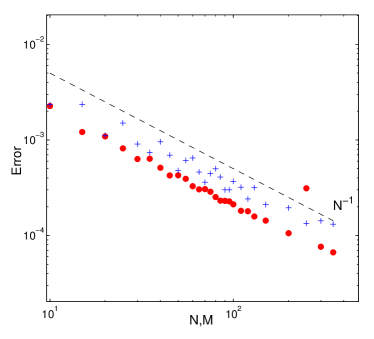
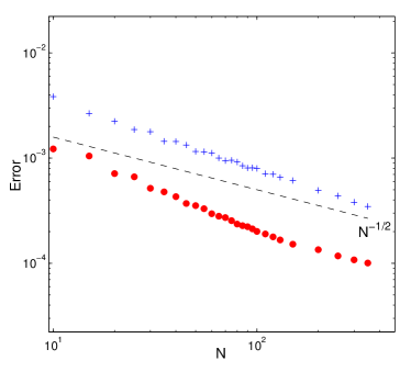
Figure 11: Convergence of the two-dimensional scattering wave function for the problem in Eq. (58) at the fixed spatial point. Left figure represents the case where the basis was increased in two dimensions simultaneously ($N=M$), right figure shows the convergence with a fixed $M=50$. Both calculations are made with $b=0.7$ and $E=2$.

Next we test the method on a model potential scattering problem described by (52) with zero partial angular momenta and the Gaussian interaction potential in the form

$$V(x,y)=-3\mathrm{e}^{-x^{2}}-3\mathrm{e}^{-y^{2}}+10\mathrm{e}^{-x^{2}-y^{2}}$$ (62)

The one-body potential, here $V_{1}(x)=-3\exp(-x^{2})$, can support one bound state. This means that using the potential (62) we can model a three-body breakup problem using the right–hand side in the form

$$\chi(x,y)=-(V(x,y)-V_{1}(x))f_{0}(x)\hat{j}_{0}(y),$$ (63)

where $f_{0}(x)$ is the wave function of the bound state, $\hat{j}_{0}(y)$ is the Riccati-Bessel function and together they represent the initial state of the system. For the considered problem there are no analytical results to compare with, so on the Figure 12 we present the solution of the linear system for $c_{nm}$ and the spatial wave function, reconstructed from $c_{nm}$ by applying the transformation matrix $W\otimes W$. On both figures we can clearly recognize the patterns of elastic scattering (the plane waves along the axes) and the breakup (the radial waves with lower frequency as part of the energy was spent to break the bound state). The in-depth analysis of the three–body scattering results is the subject of future work.

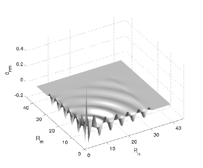
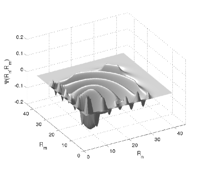
Figure 12: The solution of three–body scattering problem in oscillator representation (left figure) and the reconstructed spatial wave function (right figure). The calculation is made with $b=1$ and $E=1$. The problem has Dirichlet boundaries on all sides.

6 Conclusions and outlook

This paper focuses on scattering calculations in the oscillator representation, where the solution is expanded in the eigenstates of the harmonic oscillator. The oscillator representation is not the most natural representation to describe scattering processes since it involves a basis set that is designed to describe bound states. This leads to a rather low convergence and may result in a linear system with very large dense matrix. It is often more natural to describe a scattering process with the help of a grid representation. These grid–based calculations have been very successful in describing scattering and breakup processes in atomic and molecular physics. The Helmholtz equation is also efficiently solved on these grids.

However, internal structure of the nuclear clusters and other many–particle systems are efficiently described by such an oscillator basis, since the bottom of the potential can be mimicked by the oscillator potential leading to an efficient description of the internal structure.

In this paper we combine the advantages of grid–based calculations with those of the oscillator representation. The method was originally proposed in [33], as a further development of the $J$-matrix or algebraic method for scattering. There the method combined the grid and oscillator representation with a low–order asymptotic formula. In this paper we have improved this matching with a higher–order approximation and this brings the overall error down to the level of the discretization error of the finite–difference grid.

Although a similar asymptotic formula appeared earlier in the work of S. Igashov [34], we believe that the asymptotic formula presented in the current paper is more generally applicable. Furthermore, we have used the asymptotic formulas to improve the accuracy and convergence of the hybrid simulation method. The convergence of the method is illustrated with various examples from two–body and three–body scattering.

In preparation of this papers, our initial efforts involved application of the strategy showed in Figure 2 with the higher–order formula. However, this required the use of a forward and backward stencils to estimate the third derivative in the first grid point of the finite difference representation. This strategy, however, gives rise to eigen modes with a negative energy localized near the interface. This destroys the positive definiteness of the Laplace operator. These modes are avoided in the proposed method that uses a symmetric stencil around the matching point. This gives satisfactory convergence.

We have applied the asymptotic technique to radial oscillator state that are based on Laguerre polynomials. Similar results can be derived for the 1D oscillator states that are based on the Hermite polynomials. These Hermite polynomials are closely related to Gaussian Type Orbitals (GTO) that are frequently used in computational quantum chemistry [40] . It is worth to explore if the asymptotic formulas make it possible to combine GTO’s with grid based calculations to describe molecular scattering processes.

In the future further research is necessary on asymptotic expressions of products of two functions. This will involve convolution integrals. Better expressions for products will also help to take into account asymptotic behavior of the potentials in the grid representation.

7 Acknowledgments

We acknowledge fruitful discussions with F. Arickx and J. Broeckhove and we are grateful to B. Reps and P. Kłosiewicz for reading the manuscript. We also thank the anonymous referees for their suggestions. We are thankful for support from FWO–Flanders with project number G.0120.08.

References

- Pfannkuche et al. [1993] D. Pfannkuche, V. Gudmundsson, P. A. Maksym, Comparison of a Hartree, a Hartree-Fock, and an exact treatment of quantum-dot helium, Phys. Rev. B 47 (1993) 2244–2250.
- Sako and Diercksen [2003] T. Sako, G. Diercksen, Confined quantum systems: a comparison of the spectral properties of the two-electron quantum dot, the negative hydrogen ion and the helium atom, Journal of Physics B: Atomic, Molecular and Optical Physics 36 (2003) 1681.
- Kvaal [2009] S. Kvaal, Harmonic oscillator eigenfunction expansions, quantum dots, and effective interactions, Phys. Rev. B 80 (2009) 045321.
- Filippov and Okhrimenko [1980] G. Filippov, I. Okhrimenko, Use of an oscillator basis for solving continuum problems, Sov. J. Nucl. Phys.) 32 (1980) 480.
- Vasilevsky et al. [2001] V. Vasilevsky, A. V. Nesterov, F. Arickx, J. Broeckhove, Algebraic model for scattering in three-s-cluster systems. I. Theoretical background, Phys. Rev. C 63 (3) (2001) 034606 (16 pp).
- Dineykhan [1995] M. Dineykhan, Oscillator representation in quantum physics, vol. 26, Springer, 1995.
- Navrátil et al. [2000] P. Navrátil, J. P. Vary, B. R. Barrett, Large-basis ab initio no-core shell model and its application to , Phys. Rev. C 62 (2000) 054311, URL http://link.aps.org/doi/10.1103/PhysRevC.62.054311.
- Heller and Yamani [1974a] E. Heller, H. Yamani, New L2 approach to quantum scattering: Theory, Physical Review A 9 (3) (1974a) 1201.
- Heller and Yamani [1974b] E. Heller, H. Yamani, J-matrix method: Application to s-wave electron-hydrogen scattering, Physical Review A 9 (3) (1974b) 1209–1214.
- Alhaidari et al. [2008] A. Alhaidari, E. Heller, H. Yamani, M. E. Abdelmonem, The J-Matrix Method, Springer, 2008.
- Foumouo et al. [2006] E. Foumouo, G. Kamta, G. Edah, B. Piraux, Theory of multiphoton single and double ionization of two-electron atomic systems driven by short-wavelength electric fields: An ab initio treatment, Physical Review A 74 (6) (2006) 063409.
- Konovalov and Bray [2010] D. A. Konovalov, I. Bray, Calculation of electron-impact ionization using the -matrix method, Phys. Rev. A 82 (2010) 022708.
- Filippov [1981] G. Filippov, Taking into account correct asymptotic behavior in oscillator-basis expansions, Sov. J. Nucl. Phys. 33 (1981) 808.
- Arickx et al. [1994] F. Arickx, J. Broeckhove, P. Van Leuven, V. Vasilevsky, G. Filippov, The algebraic method for the quantum theory of scattering, Amer. J. Phys. 62 (1994) 362–370.
- Okhrimenko [1984] I. Okhrimenko, Allowance for the Coulomb interaction in the framework of an algebraic version of the resonating group method, Nuclear Physics A 424 (1) (1984) 121–142.
- Vasilevsky and Arickx [1997] V. S. Vasilevsky, F. Arickx, Algebraic model for quantum scattering: Reformulation, analysis, and numerical strategies, Phys. Rev. A 55 (1) (1997) 265–286.
- Csótó [1994] A. Csótó, Three-body resonances in 6He,6Li, and 6Be, and the soft dipole mode problem of neutron halo nuclei, Physical Review C 49 (6) (1994) 3035.
- Thompson and Pinsky [1995] L. L. Thompson, P. M. Pinsky, A Galerkin least-squares finite element method for the two-dimensional Helmholtz equation, International Journal for Numerical Methods in Engineering 38 (3) (1995) 371–397, ISSN 1097-0207, URL http://dx.doi.org/10.1002/nme.1620380303.
- Babuška et al. [1995] I. Babuška, F. Ihlenburg, E. T. Paik, S. A. Sauter, A Generalized Finite Element Method for solving the Helmholtz equation in two dimensions with minimal pollution, Computer Methods in Applied Mechanics and Engineering 128 (3-4) (1995) 325 – 359, ISSN 0045-7825, URL http://www.sciencedirect.com/science/article/pii/004578259500%890X.
- Farhat et al. [2001] C. Farhat, I. Harari, L. P. Franca, The discontinuous enrichment method, Computer Methods in Applied Mechanics and Engineering 190 (48) (2001) 6455 – 6479, ISSN 0045-7825, URL http://www.sciencedirect.com/science/article/pii/S00457825010%02328.
- Farhat et al. [2003] C. Farhat, I. Harari, U. Hetmaniuk, A discontinuous Galerkin method with Lagrange multipliers for the solution of Helmholtz problems in the mid-frequency regime, Computer Methods in Applied Mechanics and Engineering 192 (11-12) (2003) 1389 – 1419, ISSN 0045-7825, URL http://www.sciencedirect.com/science/article/pii/S00457825020%06461.
- Van der Vorst [2003] H. Van der Vorst, Iterative Krylov methods for large linear systems, Cambridge Univsity Press, 2003.
- Erlangga et al. [2006] Y. Erlangga, C. Vuik, C. Oosterlee, Comparison of multigrid and incomplete LU shifted-Laplace preconditioners for the inhomogeneous Helmholtz equation, Applied numerical mathematics 56 (5) (2006) 648–666.
- McCurdy et al. [2004] C. W. McCurdy, M. Baertschy, T. N. Rescigno, Solving the three-body Coulomb breakup problem using exterior complex scaling, J. Phys. B 37 (2004) R137–187.
- Moiseyev [1998] N. Moiseyev, Quantum theory of resonances: calculating energies, widths and cross-sections by complex scaling, Physics Reports 302 (5) (1998) 211.
- Rescigno et al. [1999] T. N. Rescigno, M. Baertschy, W. A. Isaacs, C. W. McCurdy, Collisional breakup in a quantum system of three charged particles, Science 286 (5449) (1999) 2474.
- Vanroose et al. [2005] W. Vanroose, F. Martin, T. Rescigno, C. McCurdy, Complete Photo-Induced Breakup of the H2 Molecule as a Probe of Molecular Electron Correlation, Science 310 (5755) (2005) 1787.
- Berenger [1994] J. Berenger, A perfectly matched layer for the absorption of electromagnetic waves, Journal of computational physics 114 (2) (1994) 185–200.
- Chew and Weedon [1994] W. Chew, W. Weedon, A 3D perfectly matched medium from modified Maxwell’s equations with stretched coordinates, Microwave and optical technology letters 7 (13) (1994) 599–604.
- Givoli [2008] D. Givoli, Computational Absorbing Boundaries, in: S. Marburg, B. Nolte (Eds.), Computational Acoustics of Noise Propagation in Fluids - Finite and Boundary Element Methods, Springer Berlin Heidelberg, ISBN 978-3-540-77448-8, 145–166, 2008.
- Antoine et al. [2008] X. Antoine, A. Arnold, C. Besse, M. Ehrhardt, A. Schädle, A Review of Transparent and Artificial Boundary Conditions Techniques for Linear and Nonlinear Schrödinger Equations, Comm. Comp. Phys. 4 (2008) 729–796.
- Nissen et al. [2010] A. Nissen, H. Karlsson, G. Kreiss, A perfectly matched layer applied to a reactive scattering problem, The Journal of chemical physics 133 (2010) 054306.
- Bidasyuk et al. [2010] Y. Bidasyuk, W. Vanroose, J. Broeckhove, F. Arickx, V. Vasilevsky, Hybrid method (JM-ECS) combining the -matrix and exterior complex scaling methods for scattering calculations, Phys. Rev. C 82 (6) (2010) 064603.
- Igashov [2008] S. Igashov, Oscillator Basis in the J-Matrix Method: Convergence of Expansions, Asymptotics of Expansion Coefficients and Boundary Conditions, in: A. D. Alhaidari, H. A. Yamani, E. J. Heller, M. S. Abdelmonem (Eds.), The J-Matrix Method, Springer Netherlands, ISBN 978-1-4020-6073-1, 49–66, 2008.
- Gradshteyn and Ryzhik [1980] I. S. Gradshteyn, I. M. Ryzhik, Table of Integrals, Series, and Products, Academic Press, 1980.
- Vanroose et al. [2001] W. Vanroose, J. Broeckhove, F. Arickx, Modified J-Matrix Method for Scattering, Phys. Rev. Lett. 88 (2001) 10404.
- Taylor [1983] J. R. Taylor, Scattering Theory : The Quantum Theory of Non-Relativistic Collisions, R.E. Krieger Pub. Co, Malabar, Fla., 1983.
- Vallée and Soares [2010] O. Vallée, M. Soares, Airy functions and applications to physics, Imperial College Press, 2010.
- Vanroose et al. [2006] W. Vanroose, D. Horner, F. Martin, T. Rescigno, C. McCurdy, Double photoionization of aligned molecular hydrogen, Physical Review A 74 (5) (2006) 052702.
- McMurchie and Davidson [1978] L. McMurchie, E. Davidson, One-and two-electron integrals over Cartesian Gaussian functions, Journal of Computational Physics 26 (2) (1978) 218–231.