High $Q$ BPS Monopole Bags are Urchins

Jarah Evslin and Sven Bjarke Gudnason

TPCSF, Institute of High Energy Physics, CAS, P.O. Box 918-4, Beijing 100049, P.R. China
and
Racah Institute of Physics, The Hebrew University, Jerusalem 91904, Israel

Abstract

It has been known for 30 years that ’t Hooft-Polyakov monopoles of charge $Q$ greater than one cannot be spherically symmetric. 5 years ago, Bolognesi conjectured that, at some point in their moduli space, BPS monopoles can become approximately spherically symmetric in the high $Q$ limit. In this note we determine the sense in which this conjecture is correct. We consider an $SU(2)$ gauge theory with an adjoint scalar field, and numerically find configurations with $Q$ units of magnetic charge and a mass which is roughly linear in $Q$, for example in the case $Q=81$ we present a configuration whose energy exceeds the BPS bound by about $54$ percent. These approximate solutions are constructed by gluing together $Q$ cones, each of which contains a single unit of magnetic charge. In each cone, the energy is largest in the core, and so a constant energy density surface contains $Q$ peaks and thus resembles a sea urchin. We comment on some relations between a non-BPS cousin of these solutions and the dark matter halos of dwarf spherical galaxies.

1 Introduction

Within the large moduli space of solutions of BPS monopoles [1, 2, 3, 4] of charge $Q$, it is plausible that there exists a high $Q$ limiting sequence of monopoles that are spherically symmetric up to $1/Q$ corrections. However even the most qualitative features of such solutions are, as yet, unknown. In this note we will solve an easier problem, we will explicitly construct configurations in an $SU(2)$ gauge theory with an adjoint scalar whose energy slightly exceeds the BPS bound. These configurations do not provide time-independent solutions of the equations of motion, but the near saturation of the BPS bound supports a conjecture that certain qualitative features of these solutions will be shared by some true solutions. In particular, our approximate solutions become spherically symmetric in the high $Q$ limit, and so the corresponding true solutions are also asymptotically spherically symmetric.

We will construct these approximate solutions by decomposing space into $Q$ identical cones which extend from the origin, each of which asymptotically contains a unit of magnetic flux and is axially symmetric in a sense which will be made precise below. Of course, the classification of regular polyhedra implies that no decomposition of space into identical cones exists for general $Q$. Therefore the cones may not fill all of space. We will provide configurations in which the space between the cones consists of a vanishing gauge field and a continuous Higgs field, which at high $Q$ provide a contribution to the energy which decreases with $Q$, and so is subdominant with respect to the total energy of the configurations, which is proportional to $Q$.

Our problem is then reduced to the following steps. First, in Sec. 2 we will choose an Ansatz and boundary conditions for the configuration in a single cone. The finiteness of the energy fixes all of the functions in our Ansatz except for two angular functions which must be chosen. Different choices yield different energies, none of which satisfy the BPS bound but all of which satisfy the bound up to a factor which is $Q$-independent at large $Q$. This $Q$-independence, which is critical for the qualitative agreement with a BPS configuration, is achieved if we impose that the radial dependence of the solution satisfies an ODE in a single variable. Next in Sec. 3 we will explicitly solve this equation in the large and small radius limits, and discuss how these solutions grow together. In this way we are able to establish the qualitative profiles of these solutions, confirming the monopole bag description conjectured in Ref. [5]. We will then present numerical solutions of the ODE in Sec. 4. Given the large moduli space of solutions, one may wonder why approximately spherically symmetric monopoles are interesting, especially given the fact that exact solutions which are spherically symmetric up to $1/Q$ corrections are unknown. In Sec. 5 we describe the kinds of field theories in which we expect such monopoles to be the only monopoles which survive a non-BPS deformation, and provide a very speculative application of such theories.

Since Bolognesi’s groundbreaking proposal [5], the field of monopole bags has been steadily advancing with the understanding of various limiting behaviors [6] and of large $Q$ limits of Nahm transforms of bag solutions [7]. Yesterday a paper by Manton appeared on the arXiv with significant overlap with our results [8]. He found exactly BPS Bolognesi bag solutions with an approximate spherical symmetry of the type considered here. This begs the question: how we can justify presenting an approximate solution after exact solutions have appeared? Our justification is that the physical application that we have in mind in Sec. 5 is in a theory in which we expect the radial dependence to be very distorted, but under a radial deformation the cone structure of our configurations is preserved.

2 Ansatz and equations of motion

2.1 The cone

As described in the introduction, charge $Q$ magnetic monopole configurations will be constructed from $Q$ identical cones extending from the origin together with an extrapolation in the region between the cones which yields a contribution to the energy which is subdominant at large $Q$. The crucial step in the construction is therefore to provide the configuration in a single cone. The first step is to determine the size of the cone and to fit it with coordinates.

For simplicity let $Q=n^{2}$ be a perfect square. This limitation will not be relevant for our analysis of the large $Q$ regime. We will consider a cone whose core extends along the positive $z$ axis, and will let $\psi$ be the azimuthal angle

$$\tan\psi=\frac{y}{x}\ .$$ (2.1)

If we define the radius in cylindrical coordinates to be

$$\rho\equiv\sqrt{x^{2}+y^{2}}\ ,$$ (2.2)

then the cone will be defined by the condition

$$\rho\leq\sigma\frac{z}{n}\ ,$$ (2.3)

where the cone is small enough that $n^{2}$ non-overlapping copies fit inside of $\mathbb{R}^{3}$. The constant $\sigma$ parametrizes the size of the cone.

The base of each cone at a radius $r=\sqrt{x^{2}+y^{2}+z^{2}}$ is then a circle of radius $\rho=r/\sqrt{\frac{n^{2}}{\sigma^{2}}+1}\simeq\sigma r/n$ and so the area of the base of the cone is about $\pi\sigma^{2}r^{2}/n^{2}=\pi\sigma^{2}r^{2}/Q$ which is $\sigma^{2}/4Q$ times the total area at that radius, implying that $\sigma\leq 2$ in order for the area of the cones to be less or equal to the area of the spatial sphere. This is still not sufficient for the $Q$ cones to fit inside of $\mathbb{R}^{3}$. Here we are interested in the large $Q$ limit and hence we can consider the size of the base of the cone to be much much smaller than the radius of curvature of the sphere at $r$. Then the limit, which is an upper bound on the size of the cone, is given by the size of the circle which can fit inside of a hexagon. More precisely, in the large $Q$ limit the upper bound on $\sigma$ is

$$\sigma_{\rm max}=2\sqrt{\frac{A_{\rm circle}}{A_{\rm hexagon}}}=2\sqrt{\frac{\pi}{2\sqrt{3}}}\simeq 1.9\ .$$ (2.4)

Clearly such a configuration cannot hope to saturate the BPS bound, instead a qualitative agreement with a true solution leads to the requirement that it exceeds the BPS bound by a factor (of order unity) which tends to a constant in the high $Q$ limit.

2.2 The Ansatz

We will consider an $SU(2)$ gauge theory with a massless adjoint scalar $\Phi$. Furthermore, we will make the crude approximation that the configuration of the Higgs and gauge field factorizes into $z$ and $\rho/z$-dependent functions, yielding the following axially-symmetric Ansatz

$$\Phi=h(z)\left[F(\eta)\left(c\,t^{1}+s\,t^{2}\right)+\epsilon\sqrt{1-F^{2}(\eta)}\,t^{3}\right]\ ,$$ (2.5)

for the Higgs field and

$$A_{1} =\frac{\alpha(z)}{z}\left(cs\left[J(\eta)-G(\eta)\right]t^{1}+\left[c^{2}G(\eta)+s^{2}J(\eta)\right]t^{2}-sH(\eta)\,t^{3}\right)\ ,$$

$$A_{2} =\frac{\alpha(z)}{z}\left(-\left[c^{2}J(\eta)+s^{2}G(\eta)\right]t^{1}-cs\left[J(\eta)-G(\eta)\right]t^{2}+cH(\eta)\,t^{3}\right)\ ,$$

$$A_{3} =\frac{\alpha(z)}{nz}I(\eta)\left(s\,t^{1}-c\,t^{2}\right)\ ,$$ (2.6)

for the $SU(2)$ gauge field $A_{i}$ where we have defined the variables

$$\eta\equiv\frac{n\rho}{z}\in[0,\sigma]\ ,\quad\epsilon\equiv{\rm sign}(F^{\prime}(\eta))\ ,\quad c\equiv\cos\psi\ ,\quad s\equiv\sin\psi\ ,$$ (2.7)

and the functions $F$, $G$, $H$, $I$ and $J$ of $\eta$ and also $h$ and $\alpha$ of $z$.

Such solutions are invariant under a rigid axial symmetry which simultaneously rotates the vectors

$$\begin{pmatrix}x&t^{1}\\ y&t^{2}\end{pmatrix}\rightarrow\begin{pmatrix}\cos\phi&-\sin\phi\\ \sin\phi&\cos\phi\end{pmatrix}\begin{pmatrix}x&t^{1}\\ y&t^{2}\end{pmatrix}\ ,$$ (2.8)

and the potential

$$\begin{pmatrix}A_{1}\\ A_{2}\end{pmatrix}\rightarrow\begin{pmatrix}\cos\phi&\sin\phi\\ -\sin\phi&\cos\phi\end{pmatrix}\begin{pmatrix}A_{1}\\ A_{2}\end{pmatrix}\ ,$$ (2.9)

by an arbitrary angle $\phi$.

2.3 Finite energy conditions

Topological conditions

We define the charge of the magnetic monopole to be equal to the number of cones $Q=n^{2}$ in which the Abelian magnetic field $\hbox{\rm Tr}(F\Phi)$ asymptotically pointing in the outward radial direction integrates, over the base of each cone, to a single Dirac quantum $4\pi$. The configuration then will have a finite energy only if, for all sufficiently high $z$, the value of $\Phi$ on the cone’s base is in the correct topological sector. More precisely, we will demand that, at large $z$, $\Phi$ be constant on the boundary $\rho=\sigma z/n$ of the cone. Therefore the value of $\Phi$ on the base of the cone defines a map from a 2-sphere $S^{2}$, which is the $(z=\infty,\ \eta\leq\sigma)$ two-disc $D^{2}$ with its boundary identified with a point, to the space $S^{2}$ of values of $\Phi$ of constant norm $|\Phi|=v$. The topological condition is then that this map $S^{2}\rightarrow S^{2}$ be of degree one.

We will satisfy this condition by imposing that $F$ be a continuous function such that

$$0\leq F(\eta)\leq 1\ ,\hskip 19.91684ptF(0)=0\ ,\qquad F(\sigma)=0\ ,$$ (2.10)

and $F(\eta_{0})=1$ for some intermediate value $\eta_{0}$ of its argument. We will assume that the function $F$ has only one maximum on the interval $[0,\sigma]$. One function obeying this condition is

$$F(\eta)=\sin\left(\frac{\pi\eta}{\sigma}\right)\ .$$ (2.11)

We will see shortly that the analysis of the region between the cones is simplified if one requires the derivative of $F$ to be zero at $\eta=\sigma$ which can be achieved via the deformation

$$F(\eta)=\sin\left(\frac{\pi\eta}{\sigma}\right)\left(1-\frac{\eta^{\kappa}}{\sigma^{\kappa}}\right)\ ,$$ (2.12)

where $\kappa\gg 1$ is a large integer. With this deformation, $F$ needs to be rescaled so that its maximal value is equal to one. It is difficult to calculate the resulting normalization of $F$ analytically, but for $\kappa\gg 1$ the normalization constant is arbitrarily close to unity.

High $z$ asymptotics

The topological condition on the Higgs field is necessary but not sufficient for the finite energy of the configuration. The total energy is the sum of the integrals of the gauge field strength energy density $|F_{ij}|^{2}$ and the kinetic energy density of the Higgs field $|D_{i}\Phi|^{2}$. So long as the local energy density is finite, a divergence may only arise from the noncompact region $z\rightarrow\infty$, where we will demand that

$$h(\infty)=gv\ ,\qquad\alpha(\infty)=n\ ,$$ (2.13)

and so their derivatives tend to zero. The former condition is an arbitrary choice, however in the non-BPS generalizations discussed in Sec. 5 it minimizes the potential for the Higgs field. As will be clear from the analysis that follows, any different choice of limiting value for $\alpha$ will lead to a rescaled value of the finite energy conditions on the functions $G$, $H$, $I$ and $J$. The combination of the rescaling of $\alpha$ with that of the functions leads to precisely the same form of the connection, and so this reflects a simple redundancy in the parametrization of our Ansatz.

Higgs field kinetic energy

We will now impose that the total energy in each cone is finite. There are two contributions to the energy, one from the magnetic field $F_{ij}F^{ij}$ and another from the kinetic term of the Higgs field $|D_{i}\Phi|^{2}$. As both contributions are positive definite, we must demand that they are finite separately. We now begin by imposing the finiteness of the Higgs field kinetic energy.

The finiteness of the Higgs field kinetic energy places non-trivial conditions on the functions in our Ansatz. At high $z$ the Higgs field tends to a constant limit, and so its covariant derivative is at most of order $\mathcal{O}(1/z)$ and the energy density $|D_{i}\Phi|^{2}$ is therefore at most of order $\mathcal{O}(1/z^{2})$. The finiteness of the energy of the configuration is then equivalent to the vanishing of the order $\mathcal{O}(1/z^{2})$ and $\mathcal{O}(1/z^{3})$ terms of $|D_{i}\Phi|^{2}$ for each spatial index $i$ and each gauge direction. As there are three spatial directions and three gauge directions, this consists of $9$ directions, of which we will see $3$ are independent.

The axial symmetry (2.8) and (2.9) implies that the energy density is axially symmetric. Therefore it suffices to calculate the energy at $\psi=0$, corresponding to $x=\rho$ and $y=0$. This is merely to simplify the expressions in the following. The three contributions to the kinetic energy are then the squares of the quantities $D_{i}\Phi=\partial_{i}\Phi+i[A_{i},\Phi]$,

$$D_{x}\Phi|_{y=0} = \frac{\epsilon h}{z}\big{(}n|F^{\prime}|-\alpha G\sqrt{1-F^{2}}\big{)}\left(t^{1}-\frac{\epsilon F}{\sqrt{1-F^{2}}}\,t^{3}\right)\ ,$$

$$D_{y}\Phi|_{y=0} = \frac{hF}{z}\left(\frac{n}{\eta}-\alpha\left(\epsilon J\frac{\sqrt{1-F^{2}}}{F}+H\right)\right)t^{2}\ ,$$ (2.14)

$$D_{z}\Phi|_{y=0} = h^{\prime}\big{(}F\,t^{1}+\epsilon\sqrt{1-F^{2}}\,t^{3}\big{)}+\frac{\epsilon h}{z}\left(-\eta|F^{\prime}|+\frac{\alpha}{n}\sqrt{1-F^{2}}I\right)\left(t^{1}-\frac{\epsilon F}{\sqrt{1-F^{2}}}\,t^{3}\right)\ .$$

The terms of order $\mathcal{O}(1/z^{2})$ and $\mathcal{O}(1/z^{3})$ in the kinetic energy will only arise if there are terms of order $\mathcal{O}(1/z)$ in $D_{i}\Phi$. Therefore if we assume that $h-gv$ and $\alpha-n$ go to zero at least as quickly as $1/z$, then we may drop the first term in the expression for $D_{z}\Phi$ and approximate $\alpha$ by $n$ everywhere in (2.14) without affecting the divergent terms.

The $\mathcal{O}(1/z)$ terms in each of the three $D_{i}\Phi$ can then be seen to be proportional to a combination of the functions $F$, $G$, $H$, $I$ and $J$. By setting these combinations to zero, we eliminate the divergence. These three conditions can be solved to yield, for example, $G$, $H$ and $I$ as functions of $F$ and $J$, we find respectively

$$G=\frac{|F^{\prime}|}{\sqrt{1-F^{2}}}\ ,\qquad H=\frac{1}{\eta}-\epsilon J\frac{\sqrt{1-F^{2}}}{F}\ ,\qquad I=\frac{\eta|F^{\prime}|}{\sqrt{1-F^{2}}}\ .$$ (2.15)

Recall that $F(\sigma)=0$ therefore $H$ is only finite if $J(\sigma)=0$ as well, and in fact the ratio of the two needs to tend to a constant as $z$ tends to $\sigma$. $F(0)=0$ as well, and so the finiteness of $H(0)$ requires that the divergences in both terms cancel. Here $\epsilon=1$ and so

$$\lim_{\eta\to 0}\frac{J}{F}=\lim_{\eta\to 0}\frac{1}{\eta}+\mathcal{O}(1)\ .$$ (2.16)

Substituting these relations into (2.14) the $J$ dependence cancels and so we can find exact expressions for the covariant derivatives as functionals of $F$ alone

$$D_{x}\Phi|_{y=0} = \frac{hF^{\prime}}{z}(n-\alpha)\left(t^{1}-\frac{\epsilon F}{\sqrt{1-F^{2}}}\,t^{3}\right)\ ,$$

$$D_{y}\Phi|_{y=0} = \frac{hF}{z\eta}(n-\alpha)\,t^{2}\ ,$$ (2.17)

$$D_{z}\Phi|_{y=0} = h^{\prime}\big{(}F\,t^{1}+\epsilon\sqrt{1-F^{2}}\,t^{3}\big{)}-\frac{\eta}{n}D_{x}\Phi|_{y=0}\ .$$

Notice that finite energy densities require

$$\lim_{z\to 0}\frac{h}{z}<\infty\ ,\qquad\lim_{\eta\to 0}\frac{F}{\eta}<\infty\ ,$$ (2.18)

and imply in particular

$$h(0)=\alpha(0)=0\ ,$$ (2.19)

as they must be in order for $\Phi$ and $A_{i}$ to be well defined at the origin. A finite energy density at the maximum of $F$ also requires that $F^{\prime}$ vanish as quickly as $\sqrt{1-F^{2}}$.

The total Higgs kinetic energy density is found by adding the squares of the components in Eq. (2.17)

$$\rho_{\rm kin}=\frac{1}{g^{2}}\sum_{i=1}^{3}\hbox{\rm Tr}|D_{i}\Phi|^{2}=\frac{1}{2g^{2}}(h^{\prime})^{2}+\frac{h^{2}}{2g^{2}z^{2}}(n-\alpha)^{2}\left(\frac{F^{2}}{\eta^{2}}+\frac{(F^{\prime})^{2}}{1-F^{2}}\left(1+\frac{\eta^{2}}{n^{2}}\right)\right)\ .$$ (2.20)

As the covariant derivatives were independent of $J$, so is the total kinetic energy density.

Magnetic field kinetic energy

As was the case for the Higgs kinetic term, the axial symmetry of the energy means that, for the purposes of calculating energy, it suffices to consider the gauge field strength

$$F_{ij}=\partial_{i}A_{j}-\partial_{j}A_{i}+i[A_{i},A_{j}]\ ,$$ (2.21)

at $y=0$. Again this contribution to the total energy will be finite if the energy density is at most of order $\mathcal{O}(1/z^{4})$, which means that the field strength itself must be at most of order $\mathcal{O}(1/z^{2})$. Therefore it will again suffice to impose that terms of order $\mathcal{O}(1/z)$ vanish, and that the coefficient of the order $\mathcal{O}(1/z^{2})$ terms is finite.

These conditions are only nontrivial in the case of $F_{12}$, which is

$$F_{12}|_{y=0}=\frac{\alpha}{z^{2}}\left(\left[n\left(-J^{\prime}+\frac{G-J}{\eta}\right)-\alpha GH\right]t^{1}+\left[n\left(H^{\prime}+\frac{H}{\eta}\right)-\alpha GJ\right]t^{3}\right)\ .$$ (2.22)

A divergence at the tip of the cone can be avoided if

$$\lim_{z\to 0}\frac{\alpha}{z^{2}}<\infty\ .$$ (2.23)

The expression (2.22) is then, at any constant $\eta$, of order $\mathcal{O}(1/z^{2})$ and so the energy is only divergent if the field strength itself diverges. To avoid such a divergence as $\eta$ tends to $0$ we will impose that the two quotients by $\eta$ are finite

$$\lim_{\eta\to 0}\frac{G-J}{\eta}<\infty\ ,\qquad\lim_{\eta\to 0}\frac{H}{\eta}=\lim_{\eta\to 0}\left(\frac{1}{\eta^{2}}-\frac{J\sqrt{1-F^{2}}}{\eta F}\right)<\infty\ ,$$ (2.24)

where we have used the expression for $H$ in Eq. (2.15). From here we learn that $G(0)=J(0)$, $H(0)=0$ and also this yields a refinement of the boundary condition (2.16)

$$\lim_{\eta\to 0}\frac{J}{F}=\lim_{\eta\to 0}\frac{1}{\eta}+\mathcal{O}(\eta)\ .$$ (2.25)

If we now expand $F$ as

$$F\sim c_{j}\eta^{j}+\mathcal{O}\left(\eta^{j+1}\right)\ ,$$ (2.26)

where $j=1,2,3,\ldots$ and $j$ represents the first non-zero term in the expansion then Eq. (2.25) implies

$$J\sim c_{j}\eta^{j-1}+\mathcal{O}\left(\eta^{j+1}\right)\ .$$ (2.27)

This is sufficient for rendering $H/\eta$ finite at small $\eta$. Finally, $G\sim jc_{j}\eta^{j-1}+\cdots$ together with Eq. (2.27) implies that the first constraint of Eq. (2.24) is trivially satisfied for $j>1$ while it is also non-trivially satisfied for $j=1$ due to the matching of the coefficients of $G$ and $J$.

The other components of the field strength can be evaluated easily. Using the fact that $I=\eta G$ from Eq. (2.15) one finds the $y$ component of the magnetic field

$$F_{13}|_{y=0}=-\frac{\alpha{}^{\prime}}{z}G\,t^{2}\ ,$$ (2.28)

which yields a finite energy contribution at large $z$ since $\alpha{}^{\prime}$ is at most of order $\mathcal{O}(1/z^{2})$. A divergence is avoided at small $z$ if in addition to (2.23) one imposes

$$\lim_{z\to 0}\frac{\alpha{}^{\prime}}{z}<\infty\ .$$ (2.29)

In fact this condition follows from (2.23) if $\alpha$ is differentiable at $\eta=0$.

The final component of the magnetic field is

$$F_{23}|_{y=0}=\left[\frac{\alpha\eta}{z^{2}}\left(\frac{G-J}{\eta}-\frac{\alpha GH}{n}-J^{\prime}\right)+\frac{\alpha^{\prime}J}{z}\right]t^{1}-\left[\frac{\alpha\eta}{z^{2}}\left(-\frac{H}{\eta}+\frac{\alpha JG}{n}-H^{\prime}\right)+\frac{\alpha^{\prime}H}{z}\right]t^{3}\ .$$ (2.30)

Again the finiteness of this contribution to the energy is guaranteed by the condition Eq. (2.23).

2.4 What lies outside of the cones

To choose a consistent configuration outside of the cones, one must first determine the configuration on the boundaries of the cones. We have already imposed the boundary condition $F(\sigma)=0$ and we have seen that the finiteness of $H(\sigma)$ implies that $J(\sigma)=0$ as well. In general the shape of the region between the cones is quite complicated. However, we are only interested in an approximately BPS configuration, which we define as a series of configurations at various values of $Q$ such that at large $Q$ the energy is asymptotically proportional to $Q$. We will see in this subsection that it is therefore sufficient to consider a configuration in which the gauge field vanishes in the region between the cones, considerably simplifying our analysis.

The vanishing of the gauge field in the region between the cones means that it also vanishes on the boundaries of the cones

$$G(\sigma)=H(\sigma)=I(\sigma)=0\ .$$ (2.31)

According to Eq. (2.15), for $G(\sigma)$ and $I(\sigma)$ to vanish it is sufficient to fix

$$F{}^{\prime}(\sigma)=0\ ,$$ (2.32)

which is the reason for the modification proposed in Eq. (2.12). The vanishing of $H(\sigma)$ is only slightly more complicated. By (2.15), now with $\epsilon=-1$,

$$-\frac{1}{\sigma}=\lim_{\eta\to\sigma}\frac{J(\eta)\sqrt{1-F^{2}(\sigma)}}{F(\eta)}\ .$$ (2.33)

Since $F{}^{\prime}(\sigma)$ vanishes, so must $J{}^{\prime}(\sigma)$ and so taking yet another derivative of the numerator and denominator

$$J^{\prime}(\sigma)=0\ ,\qquad J^{\prime\prime}(\sigma)=-\frac{F^{\prime\prime}(\sigma)}{\sigma}\ .$$ (2.34)

With these choices the gauge field vanishes on the boundary and the Higgs field is equal to

$$\Phi=-h(z)\,t^{3}=-h\left(r/\sqrt{1+\sigma^{2}/n^{2}}\right)t^{3}\ .$$ (2.35)

These fields may then be easily extended to the region outside of the cones, simply by asserting that $A_{i}$ always vanishes and $\Phi$ always obeys (2.35). This choice certainly does not minimize the energy, but as we will now argue, it yields a contribution to the energy which at large $Q$ is increasingly subdominant.

Notice that the energy density between the cones is simply $|\partial_{i}\Phi|^{2}$ which depends only upon $r$. Thus it is equal to a $Q$-dependent constant multiplied by the area of a sphere of radius $1$ which is not within a cone. This area tends to a constant at large $Q$. In fact, at large $Q$ the maximal number of cones that can be packed into a finite volume approaches the maximum packing of their circular cross-sections on a plane, which is given by the ratio of the area of a unit hexagon to a unit circle $2\sqrt{3}/\pi$. The area at unit radius outside of a cone is then $8\sqrt{3}-4\pi$ and hence, integrating over the radius

$$E_{\rm out}=\frac{\left(8\sqrt{3}-4\pi\right)}{g^{2}}\int dr\,r^{2}\hbox{\rm Tr}\left|\partial_{i}\Phi\right|^{2}=\frac{\left(8\sqrt{3}-4\pi\right)}{g^{2}}\int dr\,r^{2}\left(h^{\prime}(r)\right)^{2}\ ,$$ (2.36)

yields the energy outside of the cones.

Therefore at large $Q$ the geometric factor asymptotes to a $Q$-independent constant. Also at large $Q$ the $\sigma/n$ in the argument in Eq. (2.35) becomes negligible. Therefore the only source of $Q$-dependence is in $h$ itself, which interpolates between $0$ and the $Q$-independent constant $gv$. We will argue in Sec. 3 that this interpolation occurs over a region of size of order $\mathcal{O}(\sqrt{Q})$. Therefore one expects that the derivatives will decrease, and in particular the derivative squared energy density will scale as $1/Q$. However the range of integration scales as $\sqrt{Q}$, and so one expects the total contribution to the energy between the cones to decease as $1/\sqrt{Q}$, becoming ever subdominant as compared with the BPS energy which is proportional to $Q$ itself.

2.5 The total energy and BPS equations

At an arbitrary point in space, the covariant derivatives of $\Phi$ are

$$D_{1}\Phi =\left(c^{2}X_{1}+s^{2}X_{2}\right)t^{1}+cs\left(X_{1}-X_{2}\right)t^{2}-cX_{3}t^{3}\ ,$$ (2.37)

$$D_{2}\Phi =cs\left(X_{1}-X_{2}\right)t^{1}+\left(s^{2}X_{1}+c^{2}X_{2}\right)t^{2}-sX_{3}t^{3}\ ,$$ (2.38)

$$D_{3}\Phi =\left(Z_{1}-\frac{\eta}{n}X_{1}\right)\left(ct^{1}+st^{2}\right)+\left(Z_{2}+\frac{\eta}{n}X_{3}\right)t^{3}\ ,$$ (2.39)

where we have defined the following functions

$$X_{1} \equiv\frac{hF^{\prime}}{z}\left(n-\alpha\right)\ , \quad X_{2} \equiv\frac{hF}{z\eta}\left(n-\alpha\right)\ ,\qquad X_{3}\equiv\frac{hFG}{z}\left(n-\alpha\right)\ ,$$ (2.40)

$$Z_{1} \equiv h^{\prime}F\ , \quad Z_{2} \equiv h^{\prime}\epsilon\sqrt{1-F^{2}}\ ,$$ (2.41)

and the field strength components are

$$F_{12} =\frac{n}{\eta}U_{1}\left(ct^{1}+st^{2}\right)+\frac{n}{\eta}U_{2}t^{3}\ ,$$ (2.42)

$$F_{23} =\left[c^{2}\left(WJ+U_{1}\right)+s^{2}WG\right]t^{1}+cs\left(W(J-G)+U_{1}\right)t^{2}+c\left(U_{2}-WH\right)t^{3}\ ,$$ (2.43)

$$F_{31} =cs\left(W(J-G)+U_{1}\right)t^{1}+\left[c^{2}WG+s^{2}\left(WJ+U_{1}\right)\right]t^{2}+s\left(U_{2}-WH\right)t^{3}\ ,$$ (2.44)

where we have defined

$$U_{1}\equiv\frac{\alpha}{z^{2}}\left[G-J-\eta\left(J^{\prime}+\frac{\alpha}{n}GH\right)\right]\ ,\quad U_{2}\equiv\frac{\alpha}{z^{2}}\left[H+\eta H^{\prime}-\frac{\alpha}{n}\eta GJ\right]\ ,\quad W \equiv\frac{\alpha^{\prime}}{z}\ .$$ (2.45)

The BPS equations read

$$Z_{1}-\frac{\eta}{n}X_{1}-\frac{n}{\eta}U_{1}=0\ ,\qquad Z_{2}+\frac{\eta}{n}X_{3}-\frac{n}{\eta}U_{2}=0\ ,$$ (2.46)

$$X_{1}=WJ+U_{1}\ ,\qquad X_{2}=WG\ ,\qquad X_{3}=WH-U_{2}\ .$$

while the energy density for BPS-saturated configurations reads

$$g^{2}\mathcal{H}_{\rm cone,BPS} =\epsilon^{ijk}\partial_{i}\hbox{\rm Tr}\left(F_{jk}\Phi\right)=\epsilon^{ijk}\hbox{\rm Tr}\left(F_{ij}D_{k}\Phi\right)$$

$$=\frac{n}{\eta}\left(U_{1}Z_{1}+U_{2}Z_{2}\right)+W\left(JX_{1}+GX_{2}+HX_{3}\right)\ .$$ (2.47)

The only function of $\eta$ which is not given in terms of the function $F$ is $J$.

We will in the following formally integrate the above boundary term, obtaining the correct magnetic charge. This procedure imposes some criteria on $J$. Using the relations (2.15) we obtain the topological contribution to the energy density

$$g^{2}\mathcal{H}_{\rm cone,BPS}=\frac{\alpha h^{\prime}}{z^{2}\eta}\left[(n-\alpha)\frac{\epsilon FF^{\prime}}{\sqrt{1-F^{2}}}+\frac{n\eta JF^{\prime}}{F^{2}}-\frac{n\left(J+\eta J^{\prime}\right)}{F}\right]+\frac{\alpha^{\prime}h}{z^{2}\eta}2(n-\alpha)\frac{\epsilon FF^{\prime}}{\sqrt{1-F^{2}}}\ .$$ (2.48)

The total energy of the cone is given by

$$E_{\rm cone}=\frac{2\pi}{n^{2}}\int dz\int_{0}^{\sigma}d\eta\;z^{2}\eta\,\mathcal{H}_{\rm cone}\ ,$$ (2.49)

which tells us that it will be convenient to have the energy density of the form $\frac{1}{\eta}\frac{d(\cdots)}{d\eta}$. After this integration, the BPS part of the energy depends only on the boundary data and so by Stokes’ theorem is of the form $\frac{1}{z^{2}}\frac{d(\cdots)}{dz}$. Rewriting Eq. (2.48) as discussed

$$g^{2}\mathcal{H}_{\rm cone,BPS}= \ \frac{\alpha h^{\prime}}{z^{2}\eta}\left[(n-\alpha)\partial_{\eta}\left(-\epsilon\sqrt{1-F^{2}}\right)-n\partial_{\eta}\left(\frac{\eta J}{F}\right)\right]$$

$$+\frac{\alpha^{\prime}h}{z^{2}\eta}2(n-\alpha)\partial_{\eta}\left(-\epsilon\sqrt{1-F^{2}}\right)\ ,$$ (2.50)

we see from the first and third terms that $-\epsilon\sqrt{1-F^{2}}|_{0}^{\sigma}=2$. Hence, in order to obtain a total derivative in $z$, we need to impose

$$\left.-\frac{\eta J}{F}\right|_{0}^{\sigma}=2\ .$$ (2.51)

This can be done consistently with the boundary condition (2.34) in many ways, among which we will choose

$$J=\frac{F}{\eta}\epsilon\sqrt{1-F^{2}}\ .$$ (2.52)

Carrying out first the $\eta$ integration, we obtain

$$\int_{0}^{\sigma}d\eta\;\eta\,\mathcal{H}_{\rm cone,BPS}=\frac{2\alpha h^{\prime}}{g^{2}z^{2}}(2n-\alpha)+\frac{2\alpha^{\prime}h}{g^{2}z^{2}}2(n-\alpha)=\frac{2}{g^{2}z^{2}}\partial_{z}\left[(2n-\alpha)h\alpha\right]\ ,$$ (2.53)

which can readily be integrated

$$E_{\rm cone,BPS}=\frac{4\pi}{g^{2}n^{2}}\left[(2n-\alpha)h\alpha\right]_{0}^{\infty}=\frac{4\pi v}{g}\ .$$ (2.54)

This is exactly one Dirac quantum contained in a single cone.

We will however see that we can only approximately satisfy the above BPS equations and hence we will need to calculate the total energy density

$$\mathcal{H}_{\rm cone}=\frac{1}{2g^{2}}\bigg{[} \,X_{1}^{2}+X_{2}^{2}+X_{3}^{2}+\left(Z_{1}-\frac{\eta}{n}X_{1}\right)^{2}+\left(Z_{2}+\frac{\eta}{n}X_{3}\right)^{2}$$ (2.55)

$$+\left(1+\frac{n^{2}}{\eta^{2}}\right)\left(U_{1}^{2}+U_{2}^{2}\right)+2W\left(JU_{1}-HU_{2}\right)+W^{2}\left(G^{2}+H^{2}+J^{2}\right)\bigg{]}\ ,$$

for our approximate solutions. The first five terms are the kinetic energy contributions given in Eq. (2.20).

The total energy of the monopole is then

$$E_{\rm monopole}=QE_{\rm cone}+E_{\rm out}\ .$$ (2.56)

Ideally the BPS equations could all be satisfied, in which case $E_{\rm cone}=E_{\rm cone,BPS}$, however, as we will see this does not turn out to be the case for our configuration. Hence the energy of the cone is given by Eq. (2.49) with $\mathcal{H}_{\rm cone}$ given by Eq. (2.55). This energy will necessarily exceed the BPS bound (2.54).

2.6 Radial profile

The conditions in Secs. 2.3 and 2.4 guarantee that the energy of these configurations is finite. However, a qualitative agreement with true BPS solutions is only possible if the total energy is, at large $Q$, proportional to $Q$. Such a scaling constrains the radial dependence of the Higgs field and gauge fields. There are many different choices of radial dependence which yield the correct scaling. We will choose one of the simplest, we will impose that the Bogomol’nyi equations be satisfied near the cores of the cones. More precisely, we will expand the solution as a power series in $\eta/n$ and will apply the Bogomol’nyi equations at leading order in the expansion. This will determine the radial profile functions.

If we expand the function $F$ as follows

$$F(\eta)=a\eta-\frac{1}{6}b\eta^{3}+\mathcal{O}(\eta^{5})\ ,$$ (2.57)

and choose

$$J=\frac{F}{\eta}\epsilon\sqrt{1-F^{2}}\ ,$$ (2.58)

as was suggested in Eq. (2.52), we obtain at leading order in $\eta/n$ the following ODEs

$$h(z) =\frac{\alpha^{\prime}(z)}{n-\alpha(z)}\ ,$$ (2.59)

$$h^{\prime}(z) =\frac{a^{2}\alpha(z)}{z^{2}}(2n-\alpha(z))\ ,$$ (2.60)

which can be combined into a single equation for $\alpha$

$$\frac{\alpha^{\prime\prime}(z)}{n-\alpha(z)}+\left(\frac{\alpha^{\prime}(z)}{n-\alpha(z)}\right)^{2}-\frac{a^{2}\alpha(z)}{z^{2}}(2n-\alpha(z))=0\ .$$ (2.61)

With the radial differential equation at hand we are now ready to write down all of the angular profile functions in the next subsection.

2.7 Choosing an angular profile function

Summarizing the construction of this section, given the functions $F$ and $J$ one may determine all of the angular functions in the Ansatz (2.5,2.6). The radial functions on the other hand are determined by the Bogomol’nyi equations (2.59) and (2.60) at leading order in $\eta/n$.

For instance, if $F$ is given by Eq. (2.12) and $J$ by Eq. (2.52), then the other angular functions are given by

$$G(\eta)\simeq\frac{\left|\frac{\pi}{\sigma}\cos\left(\frac{\pi\eta}{\sigma}\right)\left(1-\frac{\eta^{\kappa}}{\sigma^{\kappa}}\right)-\frac{\kappa\eta^{\kappa-1}}{\sigma^{\kappa}}\sin\left(\frac{\pi\eta}{\sigma}\right)\right|}{\sqrt{1-\sin^{2}\left(\frac{\pi\eta}{\sigma}\right)\left(1-\frac{\eta^{\kappa}}{\sigma^{\kappa}}\right)^{2}}}\ ,\quad I(\eta)=\eta\,G(\eta)\ ,\quad H(\eta)=\frac{F^{2}(\eta)}{\eta}\ ,$$ (2.62)

whose $\eta/n$ expansion contains (2.61) with

$$a=\frac{\pi}{\sigma}\ .$$ (2.63)

As we have mentioned, we will not be able to satisfy the BPS equations everywhere (or equivalently to all orders in the $\eta/n$ expansion) due to the fact that true BPS solutions do not exactly factorize. Hence, in order to measure the excess energy with respect to a true BPS configuration we need to calculate the total energy density as follows

$$g^{2}\mathcal{H}_{\rm cone}= \,\frac{1}{2}h^{\prime}(z)^{2}+\left(\frac{\sigma^{2}}{n^{2}}\mathcal{P}(\eta,\sigma)+\mathcal{Q}(\eta,\sigma)\right)\frac{h(z)^{2}\left(n-\alpha(z)\right)^{2}}{z^{2}}$$ (2.64)

$$+\mathcal{Q}(\eta,\sigma)\frac{\alpha^{\prime}(z)^{2}}{z^{2}}+\left(\frac{1}{\sigma^{2}}\mathcal{R}(\eta,\sigma)+\frac{1}{n^{2}}\mathcal{S}(\eta,\sigma)\right)\frac{\alpha(z)^{2}\left(2n-\alpha(z)\right)^{2}}{z^{4}}\ ,$$

which should be integrated over the volume of the cone as in Eq. (2.49) while the total energy is given by Eq. (2.56). All the above functions $\mathcal{P}$, $\mathcal{Q}$, $\mathcal{R}$ and $\mathcal{S}$ are defined such that their integral $\int_{0}^{\sigma}d\eta\;\eta X={\rm const}$ is independent of $\sigma$, where $X=\mathcal{P}$, $\mathcal{Q}$, $\mathcal{R}$, $\mathcal{S}$.

By evaluating the integrals over the angular functions numerically we can write the total energy for the cone

$$E_{\rm cone}\simeq\frac{2\pi}{g^{2}n^{2}}\int dz\;z^{2}\bigg{[} \,\frac{1}{4}\sigma^{2}h^{\prime}(z)^{2}+\left(1.24\frac{\sigma^{2}}{n^{2}}+3.11\right)\frac{h(z)^{2}\left(n-\alpha(z)\right)^{2}}{z^{2}}$$ (2.65)

$$+3.11\frac{\alpha^{\prime}(z)^{2}}{z^{2}}+\left(\frac{6.02}{\sigma^{2}}+\frac{1.24}{n^{2}}\right)\frac{\alpha(z)^{2}\left(2n-\alpha(z)\right)^{2}}{z^{4}}\bigg{]}\ .$$

One learns from this expression that there is a competition in energy which is determined by the value of $\sigma$. Only the first and the last term are dependent on $\sigma$ at large $n$ and the first wants $\sigma$ to be small while the last one prefers a large value of $\sigma$. It so happens that the last term wins the competition due to the fact that $h$ varies only over a fairly small fraction of the integration range while the last term is roughly $\frac{6n^{4}}{\sigma^{2}z^{2}}$ which is large for large $n$. Hence a minimization of energy leads to a value of $\sigma$ which is as large as possible, i.e. $\sigma\sim 1.9$ as found in Eq. (2.4). We will check this statement numerically in Sec. 4.

3 Asymptotics and qualitative features

As we have described, the monopole is characterized by the configuration in a single cone. This consists of two parts, an angular function $F$ which needs to be chosen as well as radial functions $\alpha$, $h$. The factorizing Ansatz (2.5,2.6) implies that the radial functions are independent of the choice of $F$. In particular the function $\alpha$ may be determined using the second order ODE (2.61) and then $h$ may be determined from $\alpha$ using Eq. (2.59).

3.1 Small $z$ asymptotic behavior

At small $z$, near the center of the monopole, the gauge and Higgs fields approach zero. These two conditions imply the boundary conditions

$$\alpha(0)=\alpha^{\prime}(0)=0\ .$$ (3.1)

In the small $z$ region, $\alpha,\alpha^{\prime}\ll n$. Therefore (2.61) may be approximated by

$$\alpha^{\prime\prime}(z)-\frac{2a^{2}n^{2}\alpha(z)}{z^{2}}=0\ .$$ (3.2)

This is a homogeneous, linear, ODE with the solution

$$\alpha(z)=k_{1}z^{e_{1}}\ ,\qquad e_{1}=\frac{1}{2}+\sqrt{\frac{1}{4}+2a^{2}n^{2}}\ .$$ (3.3)

At large $n$, corresponding to large $Q$, this implies

$$\alpha(z)\simeq k_{1}z^{\sqrt{2}an}\ .$$ (3.4)

The function $h$ can then be found from the small $z$ limit of Eq. (2.59)

$$h(z)\simeq\frac{\alpha^{\prime}(z)}{n}=\sqrt{2}ak_{1}z^{\sqrt{2}an-1}\ .$$ (3.5)

3.2 Large $z$ asymptotic behavior

Far from the monopole, a finite energy solution requires that $\alpha$ tends to $n$. It will prove convenient to define the function

$$\beta(z)\equiv n-\alpha(z)\ ,$$ (3.6)

which tends to $0$ at large $z$. Eq. (2.61) may be re-expressed in terms of $\beta$ as

$$-\frac{\beta^{\prime\prime}(z)}{\beta(z)}+\left(\frac{\beta^{\prime}(z)}{\beta(z)}\right)^{2}+\frac{a^{2}}{z^{2}}\left(\beta(z)^{2}-n^{2}\right)=0\ .$$ (3.7)

We will now assume that $\beta$ may be expanded at large $z$ such that the leading term is

$$\beta(z)=k_{2}z^{e_{2}}e^{-mz}$$ (3.8)

where $m>0$. Substituting this into (3.7) one finds

$$\frac{e_{2}-a^{2}n^{2}}{z^{2}}+\cdots=0\ ,$$ (3.9)

where the ellipsis denote exponentially suppressed terms, which may be canceled by subdominant corrections to (3.8). Therefore we demand only that the first term vanishes, fixing $e_{2}=a^{2}n^{2}$.

Again the Higgs field profile function $h$ is easily found from (2.59)

$$h(z)=-\frac{\beta^{\prime}(z)}{\beta(z)}=m-\frac{a^{2}n^{2}}{z}\ .$$ (3.10)

BPS monopoles are characterized by the boundary condition that $h$ tends asymptotically to the vacuum expectation value $gv$ (recall that we have rescaled the coupling into the scalar field). Therefore $m$ is determined entirely by this boundary condition

$$m=gv\ .$$ (3.11)

Physically, $m$ is the mass of the $W$-bosons, and the exponential decay in Eq. (3.8) is just that of a massive field. Our final asymptotic form for the function $\beta(z)$ is hence

$$\beta(z)\simeq k_{2}z^{a^{2}n^{2}}e^{-gvz}\ .$$ (3.12)

3.3 Connecting the regimes and the monopole bag

We have studied two regimes: one, at small $z$, where $\alpha\ll n$ and another, at large $z$, where $\beta=n-\alpha\ll n$. Clearly it is important to determine at what value $z=z_{0}$ the solution of (2.61) interpolates between these two regimes. Neither approximation of $z$ leads to a well-controlled expansion in the intermediate regime. However one may arrive at a qualitative understanding of the solution by imagining that both expansions are roughly correct, in the sense that will be described below, at $z_{0}$. This is potentially a dangerous assumption, but numerically we have verified that the results of this subsection are indeed correct.

We will define $z_{0}$ to be the midpoint of the function $\alpha$

$$\alpha(z_{0})=\beta(z_{0})=\frac{n}{2}\ .$$ (3.13)

Therefore the matching of the two limits yields

$$\frac{\alpha^{\prime}(z_{0})}{\alpha(z_{0})}=-\frac{\beta^{\prime}(z_{0})}{\beta(z_{0})}\ .$$ (3.14)

This relation is exact. But the consequences may be approximated by substituting the asymptotic behaviors (3.4) of $\alpha$ at small $z$ and (3.12) of $\beta$ at large $z$ which gives an estimate for

$$z_{0}\sim\frac{an}{gv}\left(\sqrt{2}+an\right)\sim\frac{a^{2}n^{2}}{gv}\ ,$$ (3.15)

where in the rightmost expression we have approximated $n\gg 1$. From this expression it is clear that the $1/z$ tail of the Higgs field gives the monopole its size $\propto n^{2}$.

The value of $z_{0}$ in Eq. (3.15) is the approximate size of the monopole, the value of the radius at which the $W$-bosons begin to fall exponentially. At charge $1$, corresponding to $n=1$, one recovers the fact that the monopole size is the inverse $W$-boson mass. However more generally it reveals, as was conjectured in Ref. [5], that the radius of the monopole is proportional to the charge $Q=n^{2}$.

One may also determine the thickness $w$ of the boundary region, the distance over which $\alpha$ tends from a value near $0$ to a value near $n$. This depends on how quickly $\alpha$ changes at the boundary $z_{0}$

$$\alpha^{\prime}(z_{0})=\sqrt{2}an\frac{\alpha(z_{0})}{z_{0}}\simeq\frac{gv}{\sqrt{2}a}$$ (3.16)

valid for $n\gg 1$. The distance over which $\alpha$ changes by $n$ units is then approximately

$$w\sim\frac{n}{\alpha^{\prime}(z_{0})}\sim\frac{\sqrt{2}an}{gv}\ .$$ (3.17)

Therefore the width of the boundary of the monopole is proportional to $n=\sqrt{Q}$, while the radius of the monopole is proportional to $n^{2}=Q$. Thus at large $n$ the walls of the monopole are much thinner than its radius, confirming a conjectured description of these solutions as monopole bags in Ref. [5]. However one should note that, given the large moduli space of solutions, it seems possible that there are other sequences of BPS solutions with approximate spherical symmetry in the large $Q$ limit but with different qualitative radial profiles, and so the bag description may not apply to them.

The boundary of the monopole is not only relatively thin, with a width $w$ much smaller than $z_{0}$ at large $n$, but also it is very sharp, as $\beta$ exponentially decays at large $z$ as seen from Eq. (3.12). As we have mentioned, this is due to the fact that the gauge field is massive. On the other hand, the massless Higgs field decays only as $\mathcal{O}(1/z)$, as seen in Eq. (3.10). Therefore the Higgs field does not exhibit such a sharp transition at the boundary of the monopole.

4 Numerical results

In this section we will provide a few numerical solutions to the ODE (2.61) illustrating the radial profile functions for the monopole. We have used a shooting method to find the solution using Eq. (3.4) as the initial condition and hence $k_{1}$ as the shooting parameter. A solution with $Q=81,n=gv=9,\sigma=1.9$ is shown in Fig. 1 and its energy density is shown in Fig. 2. This solution has a total energy which is $54\%$ higher than the BPS bound $4\pi vn^{2}/g$.

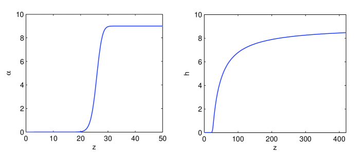
Figure 1: Left panel: the profile function $\alpha$. Right panel: the profile function $h$ both as functions of $z$ for $Q=81,n=gv=9,\sigma=1.9,z_{0}=25.8$ and $a=\pi/\sigma$.

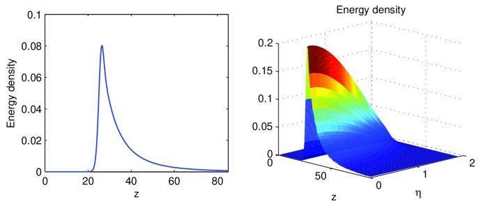
Figure 2: Left panel: the radial energy density $\int_{0}^{\sigma}d\eta\;\eta g^{2}\mathcal{H}_{\rm cone}$ as function of $z$ for the monopole with $Q=81,n=vg=9,\sigma=1.9$. Right panel: the energy density $g^{2}\mathcal{H}_{\rm cone}$ of the cone.

In order to check the size of the monopole estimated in Eq. (3.15), we have numerically calculated the value of $z_{0}$ such that $\alpha(z_{0})=n/2$ as shown in Fig. 3.

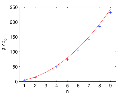
Figure 3: The approximate monopole size $gvz_{0}$ which is predicted to be $\frac{\pi}{\sigma}n\left(\sqrt{2}+\frac{\pi}{\sigma}n\right)$ and shown as the red line (we have set $\sigma=1.9$). The numerical results are shown with their corresponding errorbars.

Finally we have checked the excess energy of the solutions compared to the BPS-saturated ones which is shown in Fig. 4. The solutions turn out to exceed the BPS bound by roughly $54\%$ at large $n$.

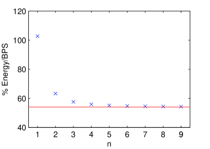
Figure 4: The total excess energy of the monopole compared to the BPS-saturated energy percentage as a function of $n=\sqrt{Q}$. It is seen that the energy excess is roughly constant at large $n$ around $54\%$.

5 Future directions

First of all we should provide a word of caution due to the fact that the BPS solutions do not share the factorization property of our configurations. For this reason we have calculated the radial profiles in terms of angular expansion parameters expanded around the origin. This means that our monopole configurations are only approximately BPS, and in particular do not provide time-independent solutions of the equations of motion. However we do believe they capture some key features of those true BPS monopoles which are spherically symmetric. As a support to this claim we found numerically that at high $Q$ the total energies of our configurations exceed that of true BPS solutions by a $Q$-independent factor of roughly $54\%$.

As we have mentioned, it may seem as though we are studying a particularly difficult and uninteresting part of the moduli space of solutions. We would however like to conjecture that in a certain class of theories it is the most interesting part:

Conjecture 1

The approximately spherically symmetric BPS monopoles are the only ones which survive the strong non-BPS deformation described below. They all reduce to the same non-BPS configuration.

Our deep interest lies in non-BPS monopoles in which a Higgs potential is included for the scalar $\Phi$. We are interested in these monopoles because of a series of perhaps coincidental facts relating $Q=1$ non-BPS monopoles with the dark matter halos of the many minimal size dwarf spheroidal galaxies which have recently been discovered in our local group, for example by the Sloan Digital Sky Survey. Some of the most striking similarities, which in fact are shared by other dark matter dominated galaxies such as larger dwarf and low surface brightness spiral galaxies, are as follows:

• Dark matter halos, like topological solitons, have a minimum mass. For solitons this corresponds to the charge $Q=1$. The lightest satellites of the Milky Way have masses of about $10^{7}\,M_{\odot}$ within 1,000 light years of their center [11] and between $10^{7}$ and $10^{8}\,M_{\odot}$ within 2,000 light years [12]. This observed minimum dark matter mass leads to the dwarf galaxy problem: For particle models of dark matter, like WIMPs, consistency with this minimum mass is a problem because simulations generally suggest 4 to 400 times more dwarf galaxies in our local group than have been observed, most of which should be much lighter than the minimum observed mass. In fact, only one dwarf galaxy (ComaBer [13]) has been observed with a mass near $10^{6}\,M_{\odot}$, and it is very elongated and irregular and appears to be in the process of being ripped apart by tidal forces.

  The existence of a topological charge, equal to one, for these small galaxies not only explains the fact that no small dwarf galaxies have been seen, but also the related fact that smaller dark matter bodies cannot exist. In this way one avoids the fatal gravitational lensing constraints faced by other MACHO dark matter models. Indeed the upper limit of the range of radii of dark matter candidates excluded by gravitational lensing is many orders of magnitude smaller than these 1000 light year solutions, and so these monopoles are too large to be excluded by the lensing bounds.

• At least in cases in which there is enough visible matter to determine the density profile, dark matter dominated galaxies and non-BPS monopoles have cores with relatively constant densities, with intermediate regions with $1/r^{2}$ densities and external regions with a faster radial fall-off. For $Q=1$ non-BPS monopoles this $1/r^{2}$ intermediate region density profile is inevitable, unlike the the higher $Q$ BPS $1/r^{2}$ density profile in the Bolognesi galaxy bags of Ref. [8] in which there are many inequivalent choices of $r$-dependence, such as solutions which the author called planets, etc.

• The cores of these non-BPS solutions in many cases naturally contain black holes [14, 15, 16, 17]. In the case of the galaxies, models often suggest that there has not been enough time to form the supermassive black holes known to inhabit most galactic cores, in addition there are even some claims of supermassive black holes without luminous galactic hosts. These problems are both naturally explained if the black hole is an integral part of the monopole solution, as it is in many models. The gradual consumption of stars, gas and dark matter particles is, in this scenario, no longer the main mechanism driving supermassive black hole formation.

• The simplest model in which non-BPS ’t Hooft-Polyakov monopoles exist is a Georgi-Glashow model with a simple Abelian Higgs quartic potential. In this case, a $Q=1$ non-Abelian monopole with the radius $r$ and mass $M$ of the smallest dwarf galaxies arises if the value of the Higgs VEV is about $v\sim\sqrt{\hbar c^{3}M/r}\sim 10^{14}\ {\rm GeV}$. This number only changes by about a factor of 2 depending on whether the luminous region is within the core or the intermediate radius regime. Had $v$ been above the Planck scale, gravity would have dominated over the Georgi-Glashow interactions and the whole solution would have been a hairy black hole instead of a dwarf galaxy. Had it been smaller than about $100\ {\rm eV}$, these monopoles could not have formed in time for dark matter to have played its crucial role in the oscillations of primordial plasma which reproduces the oscillation spectrum observed in the CMB. Given that the two physical inputs in this calculation are of galactic scales, the fact that the output is a particle physics scale in this relatively narrow acceptable window is for us miraculous. If one naively uses the rotation curves of slightly larger dwarves one may similarly conclude that the Higgs coupling is of order $\lambda\sim 10^{-97}$, had it entered $v$ with a different power, even a fourth root, the relation with dwarf galaxies would have been ruined.

• Similarly the 1,000 light year scale radii of these solutions imply that they form when the universe is about 1,000 years old [18]. Again, this is in time to help increase the intensity of fluctuations in the primordial plasma as is required by observations of the CMB. Had dwarf galactic radii been larger by a factor of 100, they would have formed too late and an inconsistency would have arisen.

• While the monopole core excluding gravity has a constant density, and with gravity may host a black hole, the core itself is nonsingular. More precisely it avoids the cusp problem of the $\Lambda CDM$ model, in which many simulations predict galactic mass distribution profiles, such as the historic Navarro, Frenk and White profile [19], with density cusps in their cores, in stark contrast with observations.

While these similarities are very strong, there is a serious problem with galaxy sized non-BPS Bolognesi bags as a dark matter candidate. Non-BPS monopoles repel, and as $v$ is less than the Planck scale this repulsion would dominate over gravity and all galaxies would be minimal dwarves and would repel one another. There is a similar problem of course for visible matter, which is mostly made of protons which also repel. In the case of protons, the solution is quite complicated. First of all there are electrons which screen the interactions between protons. While electrons have antiparticles which have the same charge as protons, for reasons which have not yet been quantitatively explained by any model, there was a primordial excess of negatively charges electrons and positively charged protons. They did not annihilate each other because they carry different conserved charges. They can combine, forming hydrogen bound states or via inverse beta decay they can even merge beyond recognition into neutrons. However, due to the choice of parameters in the standard model, the later possibility is kinematically disfavored in the conditions that have existed in most of the universe since baryogenesis.

We would like to propose that repulsion between non-BPS monopoles is avoided in a similar manner. Additional conserved charges are easily introduced in a Georgi-Glashow model by including charged fermions, which via the Jackiw-Rebbi mechanism provide an additional charge for each kind of monopole. If one adds two species of fermions, then there are two kinds of charge, which can play a role analogous to baryon number and lepton number. Monopoles of different charges can have very different masses, in fact in $\mathcal{N}=1$ supersymmetric models some flavors are usually massless while some are massive. One can then demand that the dark matter halos are made of very massive magnetically positively charged monopoles which carry one kind of flavor charge, and that the screening is caused by light negative monopoles with the other flavor charge. This eliminates the problem of galaxies repelling another.

But one still needs to worry about the stability of $Q>1$ monopoles. These will be held together by gravity. Due to the mass of the scalar field $\Phi$, the repulsive $SU(2)$ dynamics will dominate over the attractive scalar dynamics at large distances, leading to a net repulsion. The gravitational interaction in general is insufficient to counter this repulsion, as $v$ is much less than the Planck mass. However at large distances one expects the screening to play a role. Unfortunately the exact role played by this screening is highly model dependent and is not clear whether there exist any models which screen this repulsion sufficiently to allow it to be dominated by gravitational attraction, without adding any new interactions (playing the role of strong interactions in the proton analogy described above). Strong constraints on models also arise from the fact that one does not want the light monopoles to combine with the heavy monopoles, analogously to inverse beta decay, as the resulting bound state may not share the attractive features of the massive monopoles described above.

Therefore the model-independent predictions for $Q>1$ monopoles are limited by ambiguities in the screening mechanism. Nonetheless a number of very firm predictions can be made. First of all, just as the dwarf galaxy problem is a gap between the mass of globular clusters at $Q=0$ and dwarf galaxies at $Q=1$, there must also be a gap between $Q=1$ and $Q=2$. This prediction is much more general than the monopole dark matter proposal discussed in this section, but extends to any topological soliton dark matter candidate which solves the dwarf galaxy problem by identifying minimal spherical dwarf galaxies with $Q=1$ solitons. The masses of these galaxies are at best known at the 100 percent level, and so with current data such a gap cannot be verified. However one may hope that radio surveys of gas in our galactic neighborhood such as that which will be performed by the FAST telescope starting in 5 years will be able to test this claim.

Another model independent prediction is that, while the charge $Q$ is determined by the flat part of the galactic rotation curve, the radius of the core must be proportional to $\sqrt{Q}$ and, even more surprisingly, the outer radius of the region with the flat rotation curves must at large $Q$ be nearly $Q$-independent. This counter-intuitive prediction may already rule out these models, as it requires spatial extents of dwarf galaxy dark matter halos to extend far beyond their most distant stars, but it is necessary for the convexity of the galactic mass as a function of $Q$, which in turn is necessary to prevent these galaxies from exploding.

Acknowledgments

We are eternally grateful to Stefano Bolognesi and Malcolm Fairbairn for many useful and enlightening discussions. JE is supported by the Chinese Academy of Sciences Fellowship for Young International Scientists grant number 2010Y2JA01. SBG is supported by the Golda Meir Foundation Fund.

References

- [1] R. S. Ward, “A Yang-Mills Higgs Monopole of Charge 2,” Commun. Math. Phys. 79, 317-325 (1981).
- [2] M. K. Prasad, P. Rossi, “Construction Of Exact Yang-mills Higgs Multi - Monopoles Of Arbitrary Charge,” Phys. Rev. Lett. 46, 806 (1981).
- [3] M. K. Prasad, P. Rossi, “Rigorous Construction Of Exact Multi - Monopole Solutions,” Phys. Rev. D24, 2182 (1981).
- [4] M. K. Prasad, “Exact Yang-mills Higgs Monopole Solutions Of Arbitrary Topological Charge,” Commun. Math. Phys. 80, 137 (1981).
- [5] S. Bolognesi, “Multi-monopoles, magnetic bags, bions and the monopole cosmological problem,” Nucl. Phys. B752, 93-123 (2006). [hep-th/0512133].
- [6] K. -M. Lee, E. J. Weinberg, “BPS Magnetic Monopole Bags,” Phys. Rev. D79, 025013 (2009). [arXiv:0810.4962 [hep-th]].
- [7] D. Harland, “The Large N limit of the Nahm transform,” [arXiv:1102.3048 [hep-th]].
- [8] N. S. Manton, “Monopole Planets and Galaxies,” [arXiv:1111.2934 [hep-th]].
- [9] Stefano Bolognesi, Private communication in 2010.
- [10] P. Sutcliffe, “Monopoles in AdS,” JHEP 1108 (2011) 032. [arXiv:1104.1888 [hep-th]].
- [11] L. E. Strigari, J. S. Bullock, M. Kaplinghat, J. D. Simon, M. Geha, B. Willman and M. G. Walker, “A common mass scale for satellite galaxies of the Milky Way,” Nature 454 (2008) 1096 [arXiv:0808.3772 [astro-ph]].
- [12] L. E. Strigari, J. S. Bullock, M. Kaplinghat, J. Diemand, M. Kuhlen and P. Madau, “Redefining the Missing Satellites Problem,” Astrophys. J. 669 (2007) 676 [arXiv:0704.1817 [astro-ph]].
- [13] V. Belokurov et al. [SDSS Collaboration], “Cats and Dogs, Hair and A Hero: A Quintet of New Milky Way Companions,” Astrophys. J. 654 (2007) 897 [arXiv:astro-ph/0608448].
- [14] K. M. Lee, V. P. Nair and E. J. Weinberg, “A Classical instability of Reissner-Nordstrom solutions and the fate of magnetically charged black holes,” Phys. Rev. Lett. 68 (1992) 1100 [arXiv:hep-th/9111045]; K. M. Lee, V. P. Nair and E. J. Weinberg, “Black holes in magnetic monopoles,” Phys. Rev. D 45 (1992) 2751 [arXiv:hep-th/9112008]; A. Lue and E. J. Weinberg, “Magnetic monopoles near the black hole threshold,” Phys. Rev. D 60 (1999) 084025 [arXiv:hep-th/9905223].
- [15] P. Breitenlohner, P. Forgacs and D. Maison, “Gravitating monopole solutions,” Nucl. Phys. B 383 (1992) 357; P. Breitenlohner, P. Forgacs and D. Maison, “Gravitating monopole solutions. 2,” Nucl. Phys. B 442 (1995) 126 [arXiv:gr-qc/9412039].
- [16] B. Hartmann, B. Kleihaus and J. Kunz, “Gravitationally bound monopoles,” Phys. Rev. Lett. 86 (2001) 1422 [arXiv:hep-th/0009195]; B. Hartmann, B. Kleihaus and J. Kunz, “Axially symmetric monopoles and black holes in Einstein-Yang-Mills-Higgs theory,” Phys. Rev. D 65 (2002) 024027 [arXiv:hep-th/0108129].
- [17] S. Bolognesi, “Magnetic Bags and Black Holes,” [arXiv:1005.4642 [hep-th]].
- [18] T. W. B. Kibble, “Topology Of Cosmic Domains And Strings,” J. Phys. A 9 (1976) 1387.
- [19] J. F. Navarro, C. S. Frenk and S. D. M. White, “The Structure of Cold Dark Matter Halos,” Astrophys. J. 462 (1996) 563 [arXiv:astro-ph/9508025].