Dynamics of Confident Voting

Abstract

We introduce the confident voter model, in which each voter can be in one of two opinions and can additionally have two levels of commitment to an opinion — confident and unsure. Upon interacting with an agent of a different opinion, a confident voter becomes less committed, or unsure, but does not change opinion. However, an unsure agent changes opinion by interacting with an agent of a different opinion. In the mean-field limit, a population of size $N$ is quickly driven to a mixed state and remains close to this state before consensus is eventually achieved in a time of the order of $\ln N$. In two dimensions, the distribution of consensus times is characterized by two distinct times — one that scales linearly with $N$ and another that appears to scale as $N^{3/2}$. The longer time arises from configurations that fall into long-lived states that consist of two (or more) single-opinion stripes before consensus is reached. These stripe states arise from an effective surface tension between domains of different opinions.

1 INTRODUCTION

The voter model [1] describes the evolution toward consensus in a population of $N$ agents, each of which can be in one of two possible opinion states. In an update event, a randomly-selected voter adopts the state of a randomly-selected neighbor. As a result of repeated update events, a finite population necessarily reaches consensus in a time $T_{N}$ that scales as a power law in $N$ (with a logarithmic correction in two dimensions) [1, 2]. Because of its simplicity and its natural connection to opinion dynamics, the voter model has been extensively investigated (see, e.g., [3, 4]). The connection with social phenomena has also motivated efforts to extend the voter model to incorporate various aspects of social reality, such as, among others, stubbornness/contrarianism [5, 6, 7, 8], multiple states [9, 10], internal dissonance [11], individual heterogeneity [12], environmental heterogeneity [13, 14, 15, 16], vacillation [17], and non-linear interactions [18, 19]. These studies have uncovered many new phenomena that are still being actively explored.

Our investigation was initially motivated by recent social experiments of Centola [20], who studied the spread of a specific behavior in a controlled online network where reinforcement played a crucial role. Reinforcement means that an individual adopts a particular state only after receiving multiple prompts to adopt this behavior from socially-connected neighbors. These experiments found that social reinforcement played a decisive role in determining how a new behavior is adopted [20].

Previous research that has a connection with this type of reinforcement mechanism include the q-voter model [19], where multiple same-opinion neighbors initiate change, the naming game, and the AB model [21]. An example that is perhaps most closely connected to reinforcement arises in the noise-reduced voter model [22], where a voter keeps a running total of inputs towards changing opinions, but actually changes opinions only when this counter reaches a predefined threshold. A similar notion of reinforcement arises in a model of fad and innovation dynamics [23] and in a model of contagion spread [24]. The use of multiple discrete opinions is not the only option for incorporating varying opinion strength. Previous models have used a continuous range of opinions quantifying the tendency for an agent to change its opinion. [25] For example, in the bounded confidence model, an agent can possesses an opinion in a continuous range, with the spatial distance between points representing the difference in those opinions. [26]

In this paper, we study how reinforcement affects the dynamics of the voter model. In ourconfident voter model, we assume that agents possess some modicum of intrinsic confidence in their beliefs and, unlike the classic voter model, need multiple prompts before changing their opinion state. We investigate a simple realization of this confident voting in which each opinion state is further demarcated into two substates of different confidence levels. The basic variables are thus the opinion of each voter and the confidence level with which this opinion is held. For concreteness, we label the two opinion states as plus (P) and minus (M). Thus the possible states of an agent are $P_{0}$ and $P_{1}$ for confident and unsure plus agents, respectively, and correspondingly $M_{0}$ and $M_{1}$ for minus agents (Fig. 1). The new feature of confident voting is that a confident agent does not change opinion by interacting with an agent of a different opinion. Instead such an agent changes from being confident to being unsure of his opinion. On the other hand, an unsure agent changes opinion by interacting with any agent of the other opinion, as in the classic voter model.

We define two variants of confident voting that accord with common anecdotal experience (Fig. 1). In the marginal version, an unsure agent that changes opinion still remains unsure. Such an agent is often labelled a “flip-flopper”, a routinely-invoked moniker by American politicians to characterize political opponents. Figuratively, an agent who switches opinion remains ambivalent about the new opinion state and can switch back. In the extremal version, an unsure agent becomes confident after an opinion change. Such an agent “sees the light” and therefore becomes fully committed to the new opinion state. This behavior is typified by Paul the Apostle, who switched from being dedicated to finding and persecuting early Christians to embracing Christianity after experiencing a vision of Jesus.

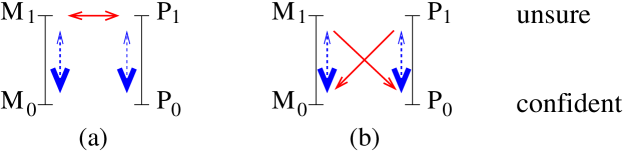
Figure 1: Illustration of the states and possible transitions in the: (a) marginal, and (b) extremal versions of the confident voter model. Dashed arrows indicate possible confidence level changes (biased toward higher confidence), while solid arrows indicate possible opinion change events.

2 MEAN-FIELD DESCRIPTION

The basic variables are the densities of the four types of agents. We use $P_{0},P_{1},M_{0},M_{1}$ to denote both the agent types and their densities. In the mean-field description, a pair of agents is randomly selected, and the state of one the two agents, chosen equiprobably, changes according to the voter-like dynamics illustrated in Fig. 1. We now outline the time evolution for the two variations of the confident voter model.

2.1 Marginal Version

For writing the rate equations, we first enumerate the possible outcomes when a pair of agents interact:

• $M_{1}P_{1}$ $\to$ $M_{1}M_{1}$ or $P_{1}P_{1}$;      $M_{0}P_{0}$   $\to$ $M_{0}P_{1}$  or $M_{1}P_{0}$;

• $P_{0}\,P_{1}$  $\to$ $P_{0}\,P_{1}$    or $P_{0}P_{0}$;      $M_{0}M_{1}$ $\to$ $M_{0}M_{1}$ or $M_{0}M_{0}$;

• $M_{1}P_{0}$ $\to$ $M_{1}P_{1}$   or $P_{0}P_{1}$;      $M_{0}P_{1}$    $\to$ $M_{1}P_{1}$  or $M_{0}M_{1}$.

That is, the interaction between two unsure agents of opposite opinions ($M_{1}P_{1}$) leads to no net density change, as in the classic voter model. However, when two confident agents of different opinions meet ($M_{0}\,P_{0}$), one of the agents becomes unsure. The next two lines account for interactions between agents of the same opinion but different confidence levels. We assume that an unsure agent exerts no influence on a confident agent by virtue of the latter being confident, while a confident agent is persuasive and converts an unsure agent to confident. Finally, the last line accounts for an unsure agent changing opinion upon interacting with a confident agent of a different opinion.

The corresponding rate equations are:

$$\dot{P}_{0} =-(M_{0}+M_{1})P_{0}+P_{0}P_{1}\equiv-MP_{0}+P_{0}P_{1}\,,$$ (1)

$$\dot{P}_{1} =~{}~{}MP_{0}-P_{0}P_{1}+(M_{1}P_{0}-M_{0}P_{1})\,,$$

with parallel equations for $M_{0}$ and $M_{1}$ that are obtained by interchanging $M\leftrightarrow P$ in Eq. (1). The rate equation for the total density of plus agents is

$$\dot{P}=M_{1}P_{0}-M_{0}P_{1},$$

and from the complementary equation for $\dot{M}$, it is evident that the total density of agents is conserved, $\dot{P}+\dot{M}=0$.

2.2 Extremal Version

For the extremal version, we again enumerate the possible outcomes when a pair of agents interact. These are:

• $M_{1}\,P_{1}$   $\to\,$ $P_{0}P_{1}$ or $M_{0}M_{1}$;       $M_{0}\,P_{0}$   $\to$ $M_{0}P_{1}$   or $M_{1}P_{0}$;

• $P_{0}\,P_{1}$      $\to$ $P_{0}P_{1}$  or $P_{0}P_{0}$;         $M_{0}\,M_{1}$   $\to$ $M_{0}M_{1}$  or $M_{0}M_{0}$;

• $M_{1}\,P_{0}$   $\to$ $M_{1}P_{1}$ or $P_{0}P_{0}$;         $M_{0}\,P_{1}$    $\to$ $M_{1}P_{1}$   or $M_{0}M_{0}$.

The point of departure, compared to the marginal version, is that a voter is now confident in its new opinion state upon changing opinion. The rate equations corresponding to these steps are:

$$\dot{P}_{0} =-M_{0}P_{0}+M_{1}P_{1}+P_{0}P_{1}\,,$$ (2)

$$\dot{P}_{1} =~{}~{}M_{0}P_{0}-M_{1}P_{1}-P_{0}P_{1}+(M_{1}P_{0}\!-\!M_{0}P_{1})\,,$$

with parallel equations for $M_{0}$ and $M_{1}$. The rate equation for the total density of plus agents is the same as that for the marginal version, so that again the total density of agents is manifestly conserved.

2.3 Time Evolution

For both variants of the confident voter model, the time evolution is dominated by the presence of a saddle point that corresponds not to consensus, but a balance between plus and minus agents. For nearly-symmetric initial conditions, the densities of the different species are initially attracted to this unstable fixed point, but eventually flow to a stable fixed point that corresponds to consensus. However when the initial condition is perfectly symmetric between plus and minus agents, then the population is driven to a mixed state that corresponds to the symmetric saddle point (Fig. 2).

2.3.1 Symmetric System

It is instructive to first study the initial conditions $M_{0}(0)=P_{0}(0)=1/2$ and $M_{1}(0)=P_{1}(0)=0$. The rate equations (1) for the marginal version of confident voting now reduce to $\dot{P}_{0}=-\dot{P}_{1}=-P_{0}^{2}$, with solution

$$P_{0}(t) =P_{0}(0)/[1+P_{0}(0)t]\,,$$ (3)

$$P_{1}(t) =\frac{1}{2}-P_{0}(t)\,.$$

Thus in an initially symmetric system, confident voters are slowly eliminated because there is no mechanism for their replenishment, and all that remains asymptotically are equal densities of unsure voters.

For the extremal version of confident voting, the rate equations (2) reduce to

$$\dot{P}_{0} =-\dot{P}_{1}=P_{0}^{2}+\frac{1}{2}P_{0}-\frac{1}{4}$$

$$=-(P_{0}-\lambda_{+})(P_{0}-\lambda_{-})\,,$$

with $\lambda_{\pm}=\frac{1}{4}(-1\pm\sqrt{5})\approx 0.309,-0.809$. Because the quadratic polynomial on the right-hand side of Eq. (2.3.1) is positive for $P_{0}<\lambda_{+}$ and negative for $P_{0}>\lambda_{+}$, the fixed point at $\lambda_{+}$ is stable. Thus $P_{0}(t)$ approaches $\lambda_{+}$ exponentially in time. We solve for $P_{0}$ by a partial fraction expansion to give

$$\frac{P_{0}(t)-\lambda_{+}}{P_{0}(t)-\lambda_{-}}=\frac{P_{0}(0)-\lambda_{+}}{P_{0}(0)-\lambda_{-}}\,\,e^{-(\lambda_{+}-\lambda_{-})t}~{},$$ (5)

which indeed gives an exponential approach to the final state of $P_{0}=\frac{1}{2}-P_{1}=\lambda_{+}$. Thus all four voting states are represented in the long-time limit.

2.3.2 Non-Symmetric System

If the initial condition is slightly non-symmetric, then numerical integrations of the rate equations clearly show that the evolution of the densities turns out to be controlled by two distinct time scales — a fast time scale that is $\mathcal{O}(1)$ and a longer time scale that is $\mathcal{O}(\ln N)$, where $N$ is the population size. To incorporate $N$ in the rate equations, we interpret these equations as describing the dynamics of voters that live on a complete graph of $N\gg 1$ sites, so that every agent interacts equiprobably with any other agent. In this framework, consensus on the complete graph should be viewed as the density of a single species being equal to $1-\frac{1}{N}$ in the rate equations. Similarly, an initial small deviation $\epsilon=\frac{1}{N}$ from the symmetric initial conditions in the rate equations (i.e., $P_{0}(0)=\frac{1}{2}+\epsilon$ and $M_{0}(0)=\frac{1}{2}-\epsilon$, with $\epsilon=\frac{1}{N}$), should be interpreted as the departure from a symmetric state by a single particle on a complete graph of $N$ sites.

   

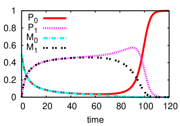
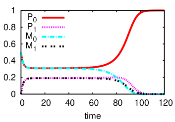
Figure 2: Evolution of the densities for the: (left) marginal and (right) extremal models with the near-symmetric initial condition $P_{0}=0.50001$, $M_{0}=0.49999$, and $P_{1}=M_{1}=0$.

In the marginal model (Fig. 2(a)), the system begins to approach the point $M_{1}=P_{1}=\frac{1}{2}$ algebraically in time, as discussed above. For a slightly asymmetric initial condition, the densities remain close to this unstable fixed point for a time that numerical integration shows is of order $\ln N$. Ultimately, the system is driven to the fixed point that corresponds to the initial majority opinion. For the extremal model, qualitatively similar behavior occurs, except that in the initial stages of evolution the system is quickly driven towards the fixed point at $P_{0}=M_{0}=\lambda_{+}$ and $P_{1}=\frac{1}{2}-\lambda_{+}$. This fixed point is a saddle node, with one stable and two unstable directions (Fig. 2(b)). Thus for nearly-symmetric initial conditions, the densities remain close to this fixed point for a time of the order $\ln N$, after which the densities are suddenly driven to one of the two stable fixed points, either $M_{0}=1$ or $P_{0}=1$.

    

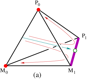
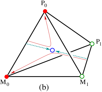
Figure 3: Composition tetrahedron for the: (a) marginal and (b) extremal models. Shown in (a) are the consensus fixed points (dots), the unstable fixed line (thick), and the symmetry line $P_{0}=M_{0}$, $P_{1}=M_{1}$ (dashed arrow) that terminates in a symmetric fixed point (circle). Shown in (b) are the unstable (circle) and stable (dots) fixed points. For both cases, two representative flows that start from nearly symmetric initial conditions are shown.

The full state space is the composition tetrahedron, which consists of the intersection of the set $\{P_{0},P_{1},M_{0},M_{1}|P_{i},M_{i}\leq 1\}$ with the normalization constraint plane $P_{0}+P_{1}+M_{0}+M_{1}=1$ (Fig. 3). Each corner corresponds to a pure system that is entirely comprised of the labeled species. For the marginal version, there are only two stable fixed points at $P_{0}=1$ and $M_{0}=1$, corresponding to consensus of either confident plus voters or confident minus voters. There is also a fixed line, defined by $P_{1}+M_{1}=1$, where the population consists only of unsure agents. This fixed line is locally unstable except at the point $P_{1}=M_{1}=\frac{1}{2}$. Thus if the system starts along the symmetry line defined by $P_{0}=M_{0}$ and $P_{1}=M_{1}$, the system flows to the final state of $P_{1}=M_{1}=\frac{1}{2}$. However, near-symmetric initial states execute a sharp U-turn and eventually flow to one of the consensus fixed points $P_{0}=1$ or $M_{0}=1$, as illustrated in Fig. 3.

For the extremal version, qualitatively similar dynamics arises, except that instead of a fixed line, there is an unstable fixed point at $P_{0}=M_{0}=\lambda_{+}$ and $P_{1}=M_{1}=\frac{1}{2}-\lambda_{+}$. Nearly symmetric initial states first flow to this unstable fixed point and remain in the vicinity of this point for a time scale that is of order $\ln N$, after which the densities quickly flow to the consensus fixed points, either $M_{0}=1$ or $P_{0}=1$.

3 CONFIDENT VOTING ON LATTICES

We now investigate confident voting dynamics when voters are situated on the sites of a finite-dimensional lattice of linear dimension $L$ (with $N=L^{d}$), with periodic boundary conditions. For the classic lattice voter model, it was found that the consensus time $T_{N}$ asymptotically scales as $N^{2}$ in one dimension $d=1$, as $N\ln N$ for $d=2$, and as $N$ for $d>2$ [1, 2]. The presence of the logarithmic factor for $d=2$ and the lack of dimension dependence for $d>2$ shows that the critical dimension $d_{c}=2$ for the classic voter model.

The confident voter model has quite different dynamics because the magnetization is not conserved, except in the symmetric limit $P_{0}=M_{0}$ and $P_{1}=M_{1}$, whereas the average magnetization is conserved in the classic voter model [1, 2]. Here the magnetization is defined as the difference in the densities of plus and minus voters of any kind. The absence of this conservation law leads to an effective surface tension between domains of plus and minus voters [22]. Consequently confident voting is closer in character to the kinetic Ising model with single-spin flip dynamics at low temperatures rather than to the classic voter model.

3.1 One Dimension

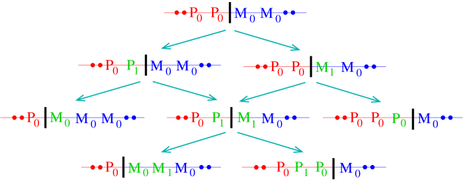
Figure 4: First three evolution steps of an interface between a $P_{0}$ and $M_{0}$ domain. Voters that change their state are shown green. After one more step, a sharp domain wall that is translated by $\pm 1$ lattice spacing is re-established.

In the simplest case of one dimension, the agents organize at long times into domains that are in a single state and the evolution is determined by the motion of the interface between two dissimilar domains. Thus we consider the evolution of a single interface between two semi-infinite domains — for example, one in state $P_{0}$ and the other in state $M_{0}$. By enumerating all possible ways that the voters at the interface can evolve (Fig. 4), we find that the domain wall moves one site to the left or to the right equiprobably after four time steps. Thus isolated interfaces between domains undergo a random walk, but with the domain wall hopping at one-fourth the rate of a symmetric nearest-neighbor random walk.

Similarly, we determine the fate of two adjacent diffusing domain walls by studying the evolution of a single voter in state $M_{0}$ in a sea of $P_{0}$ voters. By again enumerating the possible ways these two adjoining interfaces evolve, we find that the domain walls annihilate with probability $1/2$ and move apart by one lattice spacing with probability $1/2$. Additionally, we verified that the distribution of survival times for a single confident voter in a sea of opposite-opinion voters scales as $S(t)\equiv t^{-1/2}$, as in the classic voter model. We also studied the analogous single-defect initial condition for unsure voters. In all such cases, the long-time behavior is essentially the same as in the classic voter model, albeit with an overall slower time scale. Finally, we confirmed that the time to reach consensus starting from an arbitrary initial state scales quadratically with $N$. Thus the one-dimensional confident voter model at long times exhibits the same evolution as the classic voter model, but with a rescaled time.

3.2 Two Dimensions

In our simulations of confident voting in two dimensions, we typically start a population with exactly one-half of the voters in the confident plus state and one-half in the confident minus state, with their locations randomly distributed. Periodic boundary conditions are always employed. For both the marginal and the extremal versions of confident voting, $T_{N}$ appears to grow algebraically in $N$, with an exponent that is visually close to $\frac{3}{2}$ (Fig. 5). However, the local two-point slopes in the plot of $\ln T_{N}$ versus $\ln N$ are slowly and non-monotonically varying with $N$ so that it is difficult to make a precise estimate of the exponent value.

  

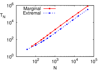
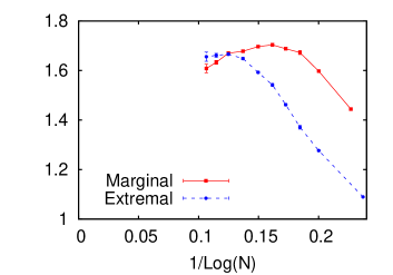
Figure 5: (left) Average consensus time $T_{N}$ on the square lattice as a function of $N$. For both models, the initial number of confident plus and minus voters are equal and randomly-distributed in space. The number of realizations for the largest system size is $40,000$. (right) Local two-point exponent for the consensus time for the marginal and extremal models. The error bars indicate the statistical uncertainty.

We argue that this slow approach to asymptotic behavior arises because there are two different routes by which consensus is achieved. For random initial conditions, most realizations reach consensus by domain coarsening, a process that ends with the formation of a large single-opinion droplet that engulfs the system. However, for a substantial fraction of realizations (roughly 38% for the extremal model and 42% for the marginal model), voters first segregate into alternating stripe-like enclaves of plus and minus voters (Fig. 6). This feature is akin to what occurs in the two-dimensional Ising model with zero-temperature Glauber dynamics, where roughly one-third of all realizations fall into a stripe state (which happens to be infinitely long lived at zero temperature [27, 28, 29]). A similar condensation into stripe states also occurs in the majority vote model [30], the $AB$ model, the naming game [21], and now the confident voter model. It is striking that this symmetry breaking occurs in a wide range of non-equilibrium systems for which the underlying dynamics is symmetric in $x$ and $y$. It is an open challenge to understand why this symmetry breaking occurs.

      

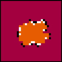
Figure 6: Typical configurations of the extremal version of the confident voter model on a $30\times 30$ square lattice that reach either a stripe state (left) or an island state (right). Black and white pixels correspond to unsure plus and minus agents; these form a sharp interface between domains of confident agents.

The existence of these two distinct modes of evolution is reflected in the probability distribution of consensus times $P(T_{N})$ (Fig. 7). Starting from the random but symmetrical initial condition, the distribution $P(T_{N})$ first has a sharp peak at a characteristic time that scales linearly with $N$, and then a distinct exponential tail whose characteristic decay time scales as $N^{3/2}$. The shorter time scale corresponds to the subset of realizations that reach consensus by conventional coarsening. For these realizations, the length scale $\ell$ of the coarsening grows as $\sqrt{t}$. When this coarsening scale reaches $L$, consensus is achieved. The consensus time is thus given by $\ell=L=\sqrt{t}$; since $N\propto L^{2}$, we have $T_{N}\simeq N$. The longer time scale stems from the subset of realizations that fall into a stripe state before consensus is eventually reached.

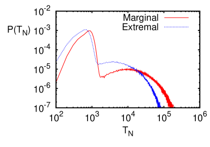
Figure 7: Consensus time distribution for a $64\times 64$ system on a double logarithmic scale. The initial condition is the same as in Fig. 5 and the data are based on 750,000 realizations.

To help understand the quantitative nature of the approach to consensus via the two different routes of coarsening and stripe states, we studied the confident voter model with the initial conditions of: (i) a large circular single-opinion island and (ii) a stripe state (Fig. 8). For the former, the initial condition is a circular region of radius $r$ that contains agents in state $M_{0}$, surrounded by agents in state $P_{0}$. For the latter, agents in state $P_{0}$ occupy the top half of the system, while the bottom half is occupied of agents in state $M_{0}$. For these two initial conditions, the consensus time $T_{N}$ grows as $N$ and as $N^{3/2}$, respectively (Fig. 8). In the latter case, the approach to asymptotic behavior is both non-monotonic and extremely slow (Fig. 8); we do not understand the mechanism responsible for these anomalies. These limiting behaviors account for the two time scales that arise in the distribution of consensus times for a system with a random, symmetric initial condition.

  

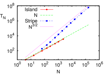
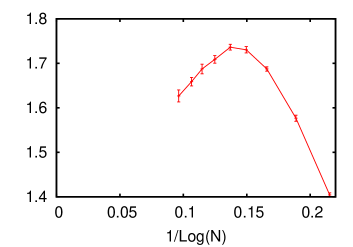
Figure 8: (left) Average consensus time for the extremal model on the square lattice as a function of the population size for: (i) island and (ii) stripe initial configurations. For the stripe initial condition, the data for the largest system size is based on 13,000 realizations. The stripe-state data has been vertically displaced for clarity. (right) The local two-point exponent for $T_{N}$ for an initial stripe state. The error bars indicate the statistical uncertainty.

Although the confident voter model has an appreciable probability of falling into a stripe state, such a state is not stable because the interface between the domains can diffuse. When the two interfaces of a stripe diffuse by a distance that is of the order of their separation, one stripe is cut in two and resulting droplet geometry quickly evolves to consensus. We estimate the time for two such interfaces to meet by following essentially the same argument as that developed for the majority vote model [30]. For a flat interface, every site on the interface can change its opinion. Such an opinion change moves the local position of the interface by $\pm 1$. For a smooth interface of length $L$, there will therefore be of the order of $L\pm\sqrt{L}$ opinion change events of plus to minus and vice versa. Thus the net change in the number of agents of a given opinion is of the order of $\pm\sqrt{L}$. Consequently, the average position of the interface moves by $\sqrt{L}/L=1/\sqrt{L}$. Correspondingly the diffusion coefficient $D_{L}$ of the interface scales as $1/L$. The time for two such interfaces that are separated by a distance of the order of $L$ to meet therefore scales as $L^{2}/D_{L}\sim L^{3}\sim N^{3/2}$.

In a $d$-dimensional system, the analog of two-stripe state is a two-slab state with a $(d-1)$-dimensional interface separating the slabs. Now the same argument as that give above leads to $N^{(d+1)/d}$ as the time scale for two initially flat interfaces to meet. According to this approach, the consensus time scales linearly with $N$ in the limit of $d\to\infty$, a limit that one normally associates with the mean-field limit. However, the rate equation approach gives a consensus time that grows as $\ln N$. We do not know how to resolve this dichotomy.

4 Summary

We introduced the notion of individual confidence in the context of the voter model. Our model is based on recent social experiments that point to the importance of multiple reinforcing inputs as an important influence for adopting a new opinion or behavior [20]. We studied two variants of confident voting in which an agent who has just switched opinion will be either have confidence in the new opinion — the extremal model — or be unsure of the new opinion — the marginal model. In the mean-field limit, a nearly symmetric system quickly evolves to an intermediate metastable state before finally reaching a consensus in one of the confident opinion states. This intermediate state is reached in a time of the order of one, while the time to reach consensus scales as $\ln N$.

On a two-dimensional lattice, a substantial fraction of all realizations of a random initial condition reach a long-lived stripe state before ultimate consensus is reached. This phenomenon appears ubiquitously in related opinion and spin-dynamics models [30, 27, 28, 29]) and an understanding of what underlies this dynamical symmetry-breaking is still lacking. An important consequence of the stripe states is that there are two independent times that describe the approach to consensus. The shorter time, which scales linearly with $N$, corresponds to realizations that reach consensus by domain coarsening. The longer time corresponds to realizations that get stuck in a metastable stripe state before ultimately reaching consensus.

An unexpected feature of confident voting is that the behavior in two dimensions, where the consensus time $T_{N}$ varies as a power law in $N$, is drastically different than that of the mean-field limit, where $T_{N}$ varies logarithmically with $N$. In contrast, in the classic voter model, $T_{N}\sim N\ln N$ in two dimensions, whereas the mean-field behavior is $T_{N}\sim N$. This dichotomy suggests that confident voting on the complete graph does not correspond to the limiting behavior of confident voting on a high-dimensional hypercubic lattice. Moreover the argument that $T_{N}$ on a $d$-dimensional hypercubic lattice scales as $N^{(d+1)/d}$ suggests that the upper critical dimension for confident voting is infinite.

References

- Liggett [1985] T. M. Liggett, Interacting Particle Systems (Springer, New York, 1985).
- Krapvisky [1992] P. L. Krapvisky, “Kinetics of monomer-monomer surface catalytic reactions,” Phys. Rev. A 45, 1067 (1992).
- Castellano et al. [2009a] C. Castellano, S. Fortunato, and V. Loreto, “Statistical physics of social dynamics,” Rev. Mod. Phys. 81, 591 (2009a).
- Krapivsky et al. [2010] P. L. Krapivsky, S. Redner, and E. Ben-Naim, A Kinetic View of Statistical Physics (Cambridge University Press, Cambridge, UK, 2010).
- Galam [2004] S. Galam, “Contrarian deterministic effects on opinion dynamics: “the hung elections scenario”,” Physica A: Statistical Mechanics and its Applications 333, 453 (2004), ISSN 0378-4371.
- Galam and Jacobs [2007] S. Galam and F. Jacobs, “The role of inflexible minorities in the breaking of democratic opinion dynamics,” Physica A 381, 366 (2007).
- Mobilia et al. [2007] M. Mobilia, A. Petersen, and S. Redner, “On the role of zealotry in the voter model,” J. Stat. Mech p. P08029 (2007).
- Yildiz et al. [2011] E. Yildiz, D. Acemoglu, A. E. Ozdaglar, A. Saberi, and A. Scaglione, “Discrete Opinion Dynamics with Stubborn Agents,” SSRN eLibrary (2011).
- Vazquez and Redner [2004] F. Vazquez and S. Redner, “Ultimate fate of constrained voters,” J. Phys. A 37, 8479 (2004).
- Volovik et al. [2009] D. Volovik, M. Mobilia, and S. Redner, “Dynamics of strategic three-choice voting,” Europhys. Lett. 85, 48003 (2009).
- Page et al. [2007] S. Page, L. Sander, and C. Schneider-Mizell, “Conformity and dissonance in generalized voter models,” Journal of Statistical Physics 128, 1279 (2007), ISSN 0022-4715.
- Masuda et al. [2010] N. Masuda, N. Gibert, and S. Redner, “Heterogeneous voter models,” Phys. Rev. E 82, 010103 (2010).
- Sood and Redner [2005] V. Sood and S. Redner, “Voter model on heterogeneous graphs,” Phys. Rev. Lett. 94, 178701 (2005).
- Suchecki et al. [2005a] K. Suchecki, V. M. Eguiluz, and M. S. Miguel, “Conservation laws for the voter model in complex networks,” Europhys. Lett. 69, 228 (2005a).
- Suchecki et al. [2005b] K. Suchecki, V. M. Eguiluz, and M. San Miguel, “Voter model dynamics in complex networks: Role of dimensionality, disorder, and degree distribution,” Phys. Rev. E 72, 036132 (2005b).
- Sood et al. [2008] V. Sood, T. Antal, and S. Redner, “Voter models on heterogeneous networks,” Phys. Rev. E 77, 041121 (2008).
- Lambiotte and Redner [2008a] R. Lambiotte and S. Redner, “Dynamics of vacillating voters,” J. Stat. Mech. p. L10001 (2008a).
- Lambiotte and Redner [2008b] R. Lambiotte and S. Redner, “Dynamics of non-conservative voters,” Europhys. Lett. 82, 18007 (2008b).
- Castellano et al. [2009b] C. Castellano, M. A. Muñoz, and R. Pastor-Satorras, “Nonlinear -voter model,” Phys. Rev. E 80, 041129 (2009b).
- Centola [2010] D. Centola, “The spread of behavior in an online social network experiment,” Science 329, 1194 (2010).
- Castello et al. [2009] X. Castello, A. Baronchelli, and V. Loreto, “Consensus and ordering in language dynamics,” Eur. Phys. J. B 71, 557 (2009).
- Dall’Asta and Castellano [2007] L. Dall’Asta and C. Castellano, “Effective surface-tension in the noise-reduced voter model,” Europhys. Lett. 77, 60005 (2007).
- Krapivsky et al. [2011] P. L. Krapivsky, S. Redner, and D. Volovik, “Reinforcement-driven spread of innovations and fads,” J. Stat. Mech. (2011).
- Melnik et al. [2011] S. Melnik, J. A. Ward, J. P. Gleeson, and M. A. Porter, “Multi-stage complex contagions,” ArXiv e-prints (2011), 1111.1596.
- Martins [2012] A. C. R. Martins, “Discrete opinion models as a limit case of the coda model,” ArXiv e-prints (2012), 1201.4565v1.
- Fortunato et al. [2005] S. Fortunato, V. Latora, A. Pluchino, and A. Rapisarda, “Vector opinion dynamics in a bounded confidence consensus model,” Int. Jour. Mod. Phys. C 16, 1535 (2005).
- Spirin et al. [2001a] V. Spirin, P. L. Krapivsky, and S. Redner, “Fate of zero-temperature ising ferromagnets,” Phys. Rev. E 63, 036118 (2001a).
- Spirin et al. [2001b] V. Spirin, P. Krapivsky, and S. Redner, “Freezing in ising ferromagnets,” Phys. Rev. E 65, 016119 (2001b).
- Barros et al. [2009] K. Barros, P. L. Krapivsky, and S. Redner, “Freezing into stripe states in two-dimensional ferromagnets and crossing probabilities in critical percolation,” Phys. Rev. E 80, 040101 (2009).
- Chen and Redner [2005] P. Chen and S. Redner, “Majority rule in finite dimensions,” Phys. Rev. E 71, 036101 (2005).