Twist, Writhe, and Helicity in the inner penumbra of a Sunspot

Abstract

The aim of this work is the determination of the twist, writhe, and self magnetic helicity of penumbral filaments located in an inner Sunspot penumbra. To this extent, we inverted data taken with the spectropolarimeter (SP) aboard Hinode with the SIR (Stokes Inversion based on Response function) code. For the construction of a 3D geometrical model we applied a genetic algorithm minimizing the divergence of $\vec{B}$ and the net magnetohydrodynamic force, consequently a force-free solution would be reached if possible. We estimated two proxies to the magnetic helicity frequently used in literature: the force-free parameter $\alpha_{z}$ and the current helicity term $h_{c_{z}}$. We show that both proxies are only qualitative indicators of the local twist as the magnetic field in the area under study significantly departures from a force-free configuration. The local twist shows significant values only at the borders of bright penumbral filaments with opposite signs on each side. These locations are precisely correlated to large electric currents. The average twist (and writhe) of penumbral structures is very small. The spines (dark filaments in the background) show a nearly zero writhe. The writhe per unit length of the intraspines diminishes with increasing length of the tube axes. Thus, the axes of tubes related to intraspines are less wrung when the tubes are more horizontal. As the writhe of the spines is very small, we can conclude that the writhe reaches only significant values when the tube includes the border of a intraspine.

1. Introduction

Investigating the physical nature and the dynamics of penumbral filaments is essential in order to understand the structure and the evolution of sunspots and their surrounding moat regions. Many important observational aspects of penumbral filaments are well settled down, although their interpretation is still a source of debate, e.g., the brightness of penumbral filaments, the inward motion of bright penumbral grains, the Evershed flow, the Net Circular Polarization (NCP), as well as moving magnetic features in the sunspot moat. During the last few years, new observational discoveries, e.g., dark cored penumbral filaments (Scharmer et al., 2002), strong downflow patches in the mid and outer penumbra (Ichimoto et al., 2007a), penumbral micro-jets (Katsukawa et al., 2007; Jur$\check{c}$ák & Katsukawa, 2008), or twisting motions of penumbral filaments (Scharmer et al., 2002; Rimmele & Marino, 2006; Ichimoto et al., 2007b; Ning et al., 2009) broadened the number of unknowns and gave new impulse to the investigation of sunspots. For recent reviews see Borrero (2011), Bellot Rubio (2010), Borrero (2009), Schlichenmaier (2009), or Tritschler (2009). An especially controversial issue is the study of the twisting motions of penumbral filaments. On the one hand, Ichimoto et al. (2007b) consider twisting motions as an apparent phenomenon, produced by lateral motions of intensity fluctuations associated with overturning convection. On the other hand, Ryutova et al. (2008) propose that the observed twist is an intrinsic property of penumbral filaments and is produced as a consequence of reconnection processes which take place in the penumbra. Su et al. (2008, 2010) conclude that the twist of penumbral filaments changes with time caused by an unwinding process.

In the present paper we study the twist of filaments of the inner penumbra of a sunspot by means of the magnetic helicity. We take advantage of the 3D geometrical model of a section of the inner penumbra of a sunspot described in Puschmann et al. (2010a) [hereafter, Paper I]. We use observations of the active region AR 10953 near solar disk center obtained on 1^st of May 2007 with the Hinode/SP. The inner, center side, penumbral area under study was located at an heliocentric angle $\theta$ = 4.63^∘. To derive the physical parameters of the solar atmosphere as a function of continuum optical depth, the SIR (Stokes Inversion based on Response function) inversion code (Ruiz Cobo & del Toro Iniesta, 1992) was applied to the data set. The 3D geometrical model was derived by means of a genetic algorithm that minimized the divergence of the magnetic field vector and the deviations from static equilibrium considering pressure gradients, gravity and the Lorentz force. We can not assess the unicity of the resulting model: the found solution just minimizes the divergency of the magnetic field and the modulus of the net force, neglecting the contribution of the aceleration terms. For a detailed description we refer to Paper I. In Puschmann et al. (2010b) [hereafter, Paper II], we calculated the electrical current density vector $\vec{J}$ in the above mentioned area and found the horizontal component of the electrical currents $\sim 4$ times larger than the vertical component ${J}_{z}$ (thus confirming the results of Pevtsov & Peregud, 1990; Georgoulis & LaBonte, 2004). In addition, we concluded that the magnetic field at the borders of bright penumbral filaments departs from a force-free configuration (see also Zhang, 2010). These results are strongly significant considering that we have imposed that our solution minimizes the net force, including the Lorentz force, and consequently, a force free solution should be found if it were possible.

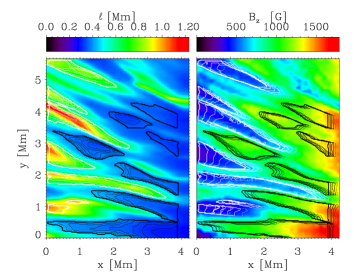
Figure 1.— Left panel: Length $\ell$ of the field lines of $\vec{B}$ integrated from the top ($z=200$ km) to the bottom layer ($z=0$ km) or until $x=4.2$ Mm. Thick isolines of equal $\ell$ define 14 areas (flux tubes) related to spines (black) and intraspines (white), respectively. Thin isolines denote different thresholds for selecting the flux tube area. Right panel: Vertical component of $\vec{B}$ at $z$ = 200 km. Contour lines correspond to horizontal cuts through the 14 flux tubes with the largest area at $z=200,150,100,50,0$ km (the thickness of each line diminishes with depth). Black and white contours distinguish between flux tubes related to spines and intraspines, respectively.

We can evaluate the magnetic field lines by the integration of $\vec{B}$ starting at each pixel of the top layer of our volume of the inner penumbra (of 4.2 Mm $\times$ 5.6 Mm $\times$ 0.2 Mm, see Paper II). In the left panel of Fig. 1 we present the length $\ell$ of each field line. As our sunspot has negative polarity, $\vec{B}$ points downwards and we thus integrate the field lines from the top layer to the bottom layer. The majority of field lines end up at the bottom layer, except the lines starting at larger X coordinates in our FOV. In the whole analized volume the magnetic field has the same polarity, and consequently, the field lines do not present maxima nor minima in our region, i.e., the field lines always travel downwards. This fact, as we will see later, simplifies the evaluation of the magnetic helicity. Areas with larger $\ell$ correspond to intraspines, since $\vec{B}$ is more horizontal, the field lines thus traverse larger distances inside our volume.

In the left panel of Fig. 1, we selected 14 areas, 7 corresponding to intraspines (thick white contours) and 7 to spines (thick black contours), according to the length $\ell$ of the magnetic field lines. For each of the selected zones we define a volume delimited by the field lines setting off from each pixel of the closed curve of the top layer. In the right panel of Fig. 1 we show the vertical component of $\vec{B}$ at $z$ = 200 km together with horizontal cuts through each of these volumes at $z=200,150,100,50,\&\,0$ km. Since the umbra is placed at the right hand side in the FOV, the cuts at deeper layers are displaced to the right. Finally we checked that the magnetic flux traversing each of the cuts is approximately constant: the standard deviation of the relative variation of the magnetic flux between the top and the bottom layer is 4.5%. Thus, each volume can be approximately considered as a flux tube.

However, the 14 areas were selected quit arbitrarily. In order to study the dependence of twist, writhe and magnetic helicity on the flux tube area, 40 additionally smaller tubes have been defined inside the larger ones (thin isolines in the left panel of Fig. 1). Thus, for most of the 14 zones we have several tubes of different size, many of them being the internal part of the larger one. Consequently, we have 54 tubes, 27 of them related to intraspines and 27 to spines.

2. Magnetic helicity, Twist, and Writhe

The study of helicity of solar magnetic features has been a hot topic during at least the last 25 years. Magnetic helicity has been investigated in solar structures at different spatial scales in the photosphere and chromosphere, as well as in the solar wind (see e.g. the reviews of Brown et al., 1999; Rust, 2002; Pevtsov & Balasubramaniam, 2003; Démoulin, 2007; Démoulin & Pariat, 2009, and references therein). The helicity in penumbral filaments has been analyzed by means of some proxies by, e.g., Ryutova et al. (2008), Tiwari et al. (2009), Su et al. (2010), and Zhang (2010).

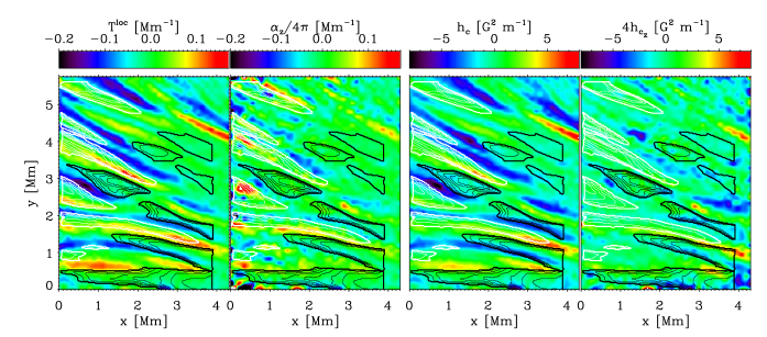
Figure 2.— From left to right: local twist ($T^{\mbox{\rm\tiny{loc}}}$), $\alpha_{z}/4\pi$, current helicity density ($h_{c}$), and $4h_{c_{z}}$ evaluated at $z=200$ km. The isolines are the same as in the left panel of Fig. 1.

The magnetic helicity, $H_{m}$, quantifies how the magnetic field is twisted, writhed, and linked. $H_{m}$ plays a key role in magneto-hydrodynamics because it is almost conserved in a plasma having a high magnetic Reynolds number (see e.g., Berger, 1984). The magnetic helicity of a vector field $\vec{B}$, fully contained within a volume $\mathcal{V}$ and bounded by a surface $\mathcal{S}$ (i.e., the normal component $B_{n}=\vec{B}\cdot\vec{n}$ vanishes at any point of $\mathcal{S}$), is (Elsasser, 1956):

$$H_{m}=\int_{\mathcal{V}}\vec{A}\cdot\vec{B}\,\,\mathrm{d}^{3}x,$$ (1)

where the vector potential $\vec{A}$ satisfies $\vec{B}=\nabla\times\vec{A}$. Berger & Field (1984) showed that Eq. 1, is not gauge-invariant if the volume of interest is not bounded by a magnetic surface, i.e., if $\vec{B}$ crosses $\mathcal{S}$ (as in the case of the volume of the penumbra retrieved from our observations). In this case the relative magnetic helicity (Finn & Antonsen, 1985) should be used:

$$H_{m}^{rel}=\int_{\mathcal{V}}(\vec{A}+\vec{A}_{p})\cdot(\vec{B}-\vec{B}_{p})\,\,\mathrm{d}^{3}x,$$ (2)

where $\vec{B}_{p}$ is a potential field having the same normal component $B_{n}$ on $\mathcal{S}$, and $\vec{A}_{p}$ is its vector potential. The relative helicity reflects twist, writhe, and linkage with respect to a current-free (potential) field, i.e., its minimum-energy state for the given $B_{n}$-condition on $\mathcal{S}$. The relative magnetic helicity so defined is gauge-invariant and has the same conservation properties and amount of topological information as the magnetic helicity. Throughout this article, the term magnetic helicity refers to the relative magnetic helicity. For an isolated magnetic flux rope, $H_{m}^{rel}$ is proportional to the sum of its twist $T$ and writhe $W$ (Berger & Field, 1984; Török et al., 2010):

$$H_{m}^{rel}=(T+W)\Phi^{2}$$ (3)

where $\Phi$ is the magnetic flux of the rope. The twist is the turning angle of a bundle of magnetic field lines around its central axis, whereas the writhe quantifies the helical deformation of the axis itself. Following Berger & Prior (2006), the twist of an infinitesimal rope is given by $T=\int T^{\mbox{\rm\tiny{loc}}}{\mathrm{d}l}$, $l$ being the arc length along the central field line of the rope and $T^{\mbox{\rm\tiny{loc}}}$ the local twist:

$$T^{\mbox{\rm\tiny{loc}}}=\frac{\mathrm{d}T}{\mathrm{d}l}=\frac{\mu_{0}J_{||}}{4\pi B_{||}}\,\,,$$ (4)

being $J_{||}$ and $B_{||}$ the components of the current and magnetic field parallel to the central field line of the rope. With this definition, $T=1$ when the field lines twist around the axis by an angle of $2\pi$ and $T^{\mbox{\rm\tiny{loc}}}$ is the local twist per unit length evaluated at a given geometrical height at each pixel. If the rope has a non-infinitesimal cross section $\Sigma$, the local twist of the rope $T^{\mbox{\rm\tiny{loc}}}_{i}$ is given by the average of the infinitesimal local twist, $T^{\mbox{\rm\tiny{loc}}}$ over $\Sigma$. Berger & Prior (2006, see also ()) give expressions for the writhe of specific geometrical configurations. Provided that the magnetic field lines in the inner penumbral region studied in this paper always travel downwards in $z$, i.e. without showing maxima nor minima between the $z_{0}=$200 km and $z_{1}=$0 km height layers, we can evaluate the writhe using a very simplified formula:

$$W=\frac{1}{2\pi}\int_{z_{0}}^{z_{1}}\frac{1}{1+|\tau_{z}|}{(\vec{\tau}\times\vec{\tau^{\prime}})}_{z}{\mathrm{d}z}\,,$$ (5)

obtained as a particular case of the more general formula of Berger & Prior (2006). In Eq. 5, $\vec{\tau}$ stands for the tangent vector to the tube axis; ${\tau_{z}}$ for the vertical component of $\vec{\tau}$; and $\vec{\tau^{\prime}}=\frac{\mathrm{d}\vec{\tau}}{\mathrm{d}z}$.

Equations 3, 4, & 5 allow the evaluation of the twist, the writhe and the magnetic helicity of an isolated tube. What happens in the case of a non-isolated tube, as is clearly the case of the penumbral tubes? The writhe of a magnetic rope, isolated or not, is a measure of the helical deformation of the axis of the rope, while the twist quantifies the winding of the magnetic field lines of the rope around its axis. The magnetic helicity measures the linking number of the field lines, averaged over all pairs of lines, and weighted by the flux (Berger & Prior, 2006; Moffatt, 1969). We can simplify the case of a non-isolated tube to a scenario in which we have just two adjoining tubes. It is clear that we can define the writhe and twist for each individual tube, and consequently its magnetic helictiy, but the helicity of the whole configuration is not just the sum of both contributions. We would need to include an extra term taking into account the linking between both tubes: the mutual helicity. Consequently the application of equations 3, 4, & 5 to our tubes retrieves only the contribution of the local values of the twist, writhe and the self helicity. The contribution of the surrounding tubes to the helicity of each flux tube is not considered. This contribution, the mutual helicity, could be larger than the self helicity (see e.g., Régnier & Priest, 2007). The mutual helicity can be calculated using the procedure described in Berger & Prior (2006). However, for the scope of this paper we limit the calculation to self helicity.

3. Proxies of the magnetic helicity

The current helicity density is defined (see e.g., Seehafer, 1990) as $h_{c}={\vec{B}}\cdot\nabla\times{\vec{B}}$. If we take as magnetic ropes the tubes defined by the field lines starting in each pixel, (being then $B_{||}=B$), Eq. 4 becomes $T^{\mbox{\rm\tiny{loc}}}=h_{c}/4\pi B^{2}$. The parameter $\alpha$ is usually defined in a force-free configuration, i.e., when ${\vec{B}}$ is parallel to its curl, by $\nabla\times{\vec{B}}$ = $\alpha{\vec{B}}$. The $\alpha$ parameter can be defined for non force-free fields: $\alpha={\vec{B}}\cdot\nabla\times{\vec{B}}/B^{2}$. This is the definition we will use throughout the paper. In order to see how this re-defined $\alpha$ differs from the force-free definition, let us decompose $\nabla\times{\vec{B}}=(\nabla\times{\vec{B}})_{||}+(\nabla\times{\vec{B}})_{\perp}$. From its definition, $\alpha$ becomes equal to $\alpha=\pm|(\nabla\times{\vec{B}})_{||}|/B$ which is equal to the classical definition for a force-free field. The $\pm$ is needed to consider the case when $(\nabla\times{\vec{B}})_{||}$ and $\vec{B}$ point in opposite direction, i.e., when $\alpha$ is negative. For a no force free-field, the parameter $\alpha$ is then the ratio between the parallel component of the curl of the magnetic field and its modulus. Evidently, in a general case, we will have $\alpha=h_{c}/B^{2}=4\pi\,T^{\mbox{\rm\tiny{loc}}}$.

Given the difficulty of empirically obtaining $H_{m}^{rel}$ and ${\vec{J}}$, one finds many works where different proxies were used. Before evaluating the magnetic helicity we can calculate, from our data, some of the most usual proxies of the magnetic helicity. Among them the most common proxies, with several different but more or less equivalent definitions, are the $\alpha_{z}=(\nabla\times{\vec{B}})_{z}/B_{z}$ parameter (see e.g., Su et al., 2009, 2010; Pevtsov et al., 2008, and references therein), and the parameter $h_{c_{z}}=B_{z}(\nabla\times{\vec{B}})_{z}$ (see e.g., Zhang, 2010). It is evident that for a force-free field $\alpha_{z}=\alpha$ and $h_{c_{z}}=\alpha B_{z}^{2}=h_{c}B_{z}^{2}/B^{2}$. That means that the $h_{c_{z}}$ parameter could be meaningless for nearly horizontal magnetic fields, such as those found in sunspot penumbrae.

Many authors suppose that the sign of the integral of $\alpha_{z}$ (or $h_{c_{z}}$) over the volume of a magnetic structure coincides with the sign of $H_{m}^{rel}$, although this fact has not yet been demonstrated (Démoulin, 2007). On the other hand, Hagyard & Pevtsov (1999) point out that $h_{c_{z}}$ only considers the vertical component $J_{z}$ of the electric current density vector, $h_{c_{z}}$ can strongly differ from $h_{c}$, provided that $J_{z}$ is much smaller than the horizontal components, at least in the inner penumbra (see Paper II). Besides, Pariat et al. (2005) comment that, since the magnetic helicity is a global quantity, it is not obvious that a helicity density has any physical meaning.

We evaluated these proxies in the inner penumbral region under study. In the left panels of Fig. 2 we present $T^{\mbox{\rm\tiny{loc}}}$ (evaluated from Eq. 4) and $\alpha_{z}/4\pi$ evaluated at each pixel at $z=200$ km. As in the inner penumbra the magnetic field is not force-free at the borders of bright penumbral filaments (see Paper II), $\alpha_{z}/4\pi$ (2^nd panel) is only qualitatively similar to $T^{\mbox{\rm\tiny{loc}}}$. In the 3^rd and 4^th panel we present $h_{c}={\vec{B}}\cdot\nabla\times{\vec{B}}$ and $h_{c_{z}}$ evaluated at $z=200$ km. $h_{c_{z}}$ is multiplied by a factor 4 just to make easier its comparison with $h_{c}$. As we have seen before, $T^{\mbox{\rm\tiny{loc}}}=h_{c}/4\pi B^{2}$, and thus the general aspect of $h_{c}$ is very similar to $T^{\mbox{\rm\tiny{loc}}}$. However, $h_{c_{z}}$ resembles $h_{c}$ only marginally (the standard deviations are $\sigma(h_{c})=2.1\,G^{2}\,m^{-1}$ and $\sigma(h_{c_{z}})=0.4\,G^{2}\,m^{-1}$). The values of $\alpha_{z}/4\pi$ and $h_{c_{z}}$ at $z=200$ km obtained here are very similar to the results found in the literature: Tiwari et al. (2009) found that $\alpha_{z}/4\pi$ varies around $\pm 0.15Mm^{-1}$ along azimuthal paths in the middle penumbra; Su et al. (2010) found a fluctuation of $\alpha_{z}/4\pi$ larger than $\pm 0.05Mm^{-1}$ over an inner penumbral region; Su et al. (2009) found that $h_{c_{z}}$ fluctuates along an azimuthal path in the inner penumbra with an amplitude larger than 1 $G^{2}\,m^{-1}$ while Balthasar & Gömöry (2008) found penumbral mean values of about 0.04 $G^{2}\,m^{-1}$. In the four panels of Fig. 2, the outlined areas were selected by different thresholds of $\ell$, the length of the magnetic field lines between the layers $z=200$ km and $z=0$ km (see also Section 1 and Fig. 1). The sign of the integral of $T^{\mbox{\rm\tiny{loc}}}$ and $\alpha_{z}/4\pi$ over the above mentioned areas only coincides in 39% of the 54 tubes (if we consider only the areas related to the intraspines this value decreases to 15% of the 27 tubes). The same figures are obtained for the percentage of coincidence between the signs of the integrals of $h_{c}$ and $h_{c_{z}}$, approximately. This weak coincidence demonstrates that, at least in the inner penumbra of a sunspot, $\alpha_{z}/4\pi$ and $h_{c_{z}}$ are not good estimates of $T^{\mbox{\rm\tiny{loc}}}$ and $h_{c}$, respectively. As already shown in Paper II, the magnetic field in the area under study significantly departures from a force-free configuration.

Note that $T^{\mbox{\rm\tiny{loc}}}$ reaches significant values only at the borders of the intraspines: these are exactly the areas where the electric current density is large (see Fig. 1 of Paper II). Furthermore, often $T^{\mbox{\rm\tiny{loc}}}$ changes its sign at both sides of bright filaments, i.e., for the majority of the intraspines, $T^{\mbox{\rm\tiny{loc}}}$ shows negative values at the upper (larger Y-coordinate) borders of the filaments and positive values at the lower borders. The alternation of the sign in the twist is also observed (although less evident) in the maps of $\alpha_{z}$ and $h_{c_{z}}$ and it is clearly visible in Tiwari et al. (2009), Su et al. (2009), Su et al. (2010), and Zhang (2010).

This phenomenon can be explained if we consider that the field lines of the magnetic background component wrap around the intraspines (Borrero et al., 2008) and tend to meet above the intraspines, thus generating a curvature of different sign in the field lines at both sides of the intraspines. Thus $T^{\mbox{\rm\tiny{loc}}}$ could be measuring the twist of the background field wrapping around the intraspines rather than the twist of the field lines of the intraspines themselves. However, the alternation of signs of the twist at both sides of a penumbral filament is compatible with the magnetohydrostatic equilibrium model of a magnetic flux tube built by Borrero (2007). This model includes a transverse component of $\vec{B}$ having opposite twist at both sides of a plane longitudinally cutting the flux tube. This model is able of explaining both the dark cored penumbral filaments and the net circular polarization observed in penumbral filaments (Borrero et al., 2007). Magara (2010) suggests the existence of an intermediate region where the magnetic field has a transitional configuration between a penumbral flux tube and the background field: in such areas, coinciding with the largest electrical current density (see Paper II), penumbral micro-jets are produced as observed by Katsukawa et al. (2007).

4. Numerical test

To check its correctness, the procedure used for the evaluation of twist, writhe, and magnetic helicity was applied to two different analytical cases. In the first case we consider that the magnetic field lines follow a helix around a vertical straight line. The magnetic field vector is defined by $\vec{B}=B_{0}\,\hat{z}+B_{1}\,r\,\hat{\theta}$ with $B_{0}$ and $B_{1}$ being constant. $\vec{B}$ could easily be decomposed in a potential $\vec{B}_{p}=B_{0}\,\hat{z}$ and a close (toroidal) field $\vec{B}_{c}=B_{1}\,r\,\hat{\theta}$. Obviously, the potential component $\vec{B}_{p}$ fulfills the conditions required in Eq. 2 in the case of a cylindrical tube: $\vec{B}$ and $\vec{B}_{p}$ have the same normal component on the external surface of the tube. The determination of the vector potential, in this case, is straightforward: $\vec{A}=B_{0}\,r/2\,\hat{\theta}-B_{1}\,r^{2}/2\,\hat{z}$. The vector potential of the potential component will be $\vec{A_{p}}=B_{0}\,r/2\,\hat{\theta}$. Using Eq. 2, the magnetic helicity of a cylindrical tube of height $L$ and radius $R$ becomes $H_{m}=\frac{1}{2}\pi\,B_{0}\,B_{1}\,R^{4}\,L$. The magnetic flux of this tube is $\Phi=\pi\,B_{0}\,R^{2}$. This tube has a zero writhe because its axis is a straight line. From Eq. 3, the twist follows as

$$T=\frac{B_{1}\,L}{2\pi\,B_{0}}.$$ (6)

This is obviously the expected result, provided that the pitch (of screw-step) of our helix is $\frac{2\pi\,B_{0}}{B_{1}}$ and the twist is a measure of the number of turns done by the magnetic field lines along a longitude $L$.

In the first four rows of Table 1 we present the analytical (i.e., using Eq. 6) and numerical results (using Eqs. 4 and 5) for tubes with $B_{0}=-0.2\,{\mbox{T}}$, $B_{1}=0.04\,{\mbox{T}}\,{\mbox{Mm}}^{-1}$, $L=0.225\,{\mbox{Mm}}$ and a radius $R$ equal to $0.2$ and $1$ Mm. We used the same spatial grid as in the observational case.

In order to check the accuracy of the determination of twist, writhe and magnetic helicity in a more general case, we carried out a second test, building a helical magnetic field that turns around a helical axis. Let us suppose that the axis of the tube is a vertical helix of radius $R_{h}$ turning an angle $\Psi$ through a length $L=0.22\,{\mbox{Mm}}$. Then, the magnetic field at the axis will be $\vec{B}=B_{0}\,\hat{z}+B_{1}\,R_{h}\,\hat{\theta}$ with $B_{1}=B_{0}\,\Psi/L$. Following Berger & Prior (2006), the writhe of a magnetic flux tube whose axis is a helix can be easily evaluated in terms of its polar writhe (i.e., area/$2\pi$ of the section of the unity sphere limited by the tantrix curve and the north pole. The tantrix curve is the path, the tip of the tangent vector takes on the unit sphere). In our case, the writhe becomes:

$$W=\frac{\Psi}{2\pi}(1-\frac{B_{0}}{|B|}).$$ (7)

Once we have the axis, we can easily build a tube with a given twist around such an axis. We chose the radius of the tube as $R=0.2$ Mm, and the radius of the helical axis as $R_{h}=0.4\,{\mbox{Mm}}$, and $B_{1}=0.5\,{\mbox{T\,Mm${}^{-1}$}}$. The angle $\Psi$ takes a value of $9.124$ degrees in order to have an analytical writhe (i.e., using Eq. 7) of $0.001$. The added twist takes the values $0.0$, $0.001$, $0.01$, $0.1$, and $-0.001$. Note that, as the magnetic helicity is proportional to the sum of twist and writhe, in the last case we will have a null magnetic helicity. The results of these tests are presented in the ten bottom rows of Table 1.

Table 1Test results: Writhe ($W$), twist ($T$), and magnetic helicity ($H_{m}$), for a helical magnetic field (first four rows) and a helical magnetic field winding around a helical axis.

$R$ [Mm]		$W$	$T$	$H_{m}\,\,[{\mbox{Mx}}^{2}]$
0.2	analytical	0.00	-7.16e-3	-4.52e+34
	numerical	-9.e-28	-7.16e-3	-4.50e+34
1.0	analytical	0.00	-7.16e-3	-2.83e+37
	numerical	-9.e-28	-7.16e-3	-2.81e+37
0.2	analytical	1.00e-3	0.00	8.16e+34
	numerical	0.99e-3	1.90e-6	8.07e+34
0.2	analytical	1.00e-3	1.00e-3	1.63e+35
	numerical	0.99e-3	1.07e-3	1.67e+35
0.2	analytical	1.00e-3	1.00e-2	8.97e+35
	numerical	0.98e-3	1.06e-2	9.47e+35
0.2	analytical	1.00e-3	1.00e-1	7.01e+36
	numerical	0.97e-3	0.99e-1	6.91e+36
0.2	analytical	1.00e-3	-1.00e-3	0.00
	numerical	0.99e-3	-1.06e-3	-6.14e+33

Figure 3.— Panel (a): Length of the axis of each flux tube. The values corresponding to tubes of the same zone are connected by lines. Cross symbols correspond to intraspines and small circles to spines. Panels (b), (c), and (d): writhe, twist, sum of writhe and twist.

Figure 4.— Panels (a) and (b): normalized twist ($T/\zeta$) and writhe ($W/\zeta$) versus the length of the axis of each flux tube $\zeta$. The absolute value $|W/\zeta|$ has been overplotted in panel (b) with triangle symbols. The dashed line is the linear fit of $|W/\zeta|$. Panel (c): wavenumber. Panel (d): $T/\zeta$ versus $\alpha/4\pi$ averaged over the section of each flux tube at $z=200$ km. Panels (e) and (f): $T$ versus the average of $\alpha_{z}/4\pi$ and $h_{c_{z}}$ respectively. In panels (d), (e) and (f) the straight line with slope 1 has been overplotted. Cross symbols correspond to intraspines and small circles to spines.

5. Results

Table 2Axis length $\zeta$, magnetic flux $\Phi$, twist, writhe and magnetic helicity for the 14 largest zones. The 7 first (last) rows are related to intraspines (spines).

index	$\zeta$ [Mm]	$\Phi$ [Mx]	T	W	$H_{m}\,\,[{\mbox{Mx}}^{2}]$
0	0.79	-3.05e+18	-0.0138	0.0258	1.11e+35
4	0.80	-1.56e+18	-0.0272	0.0182	-2.19e+34
9	1.06	-4.71e+18	-0.0210	0.0024	-4.12e+35
15	0.92	-2.55e+18	-0.0224	-0.0163	-2.51e+35
20	0.80	-5.69e+18	0.0111	0.0041	4.94e+35
23	1.02	-2.64e+17	-0.0054	0.0166	7.80e+32
25	1.00	-5.13e+17	0.0096	0.0079	4.59e+33
28	0.32	-4.43e+18	-0.0023	0.0000	-4.42e+34
29	0.33	-3.41e+18	-0.0028	0.0021	-8.34e+33
30	0.34	-6.29e+18	-0.0041	0.0011	-1.20e+35
36	0.34	-7.73e+18	-0.0065	0.0010	-3.30e+35
40	0.37	-6.30e+18	-0.0041	0.0015	-1.01e+35
41	0.36	-1.13e+19	-0.0001	0.0007	7.56e+34
46	0.35	-2.04e+19	-0.0010	-0.0017	-1.15e+36

In Table 2 we present the resulting values of the axis length, magnetic flux, twist, writhe and self magnetic helicity for the flux tubes of the 14 largest zones. As the magnetic helicity depends on the square of the magnetic flux, and our selected areas are very different in area, the resulting magnetic helicity varies over a wide range of several orders of magnitude. To study the dependence of the precedent quantities on the length of the respective axis, in Fig. 3, we plot the length of the axis of each flux tube $\zeta$, the writhe, the twist, and the sum of twist and writhe for the $54$ selected tubes related to intraspines (index ranging form $0$ to $26$) and spines (index ranging form $27$ to $53$). The values corresponding to tubes of the same zone (see left panel of Fig. 1) are connected by straight lines. As the magnetic field in the spines is more vertical than in the intraspines, the length of the axis of the tubes related to the spines is clearly shorter. For each intraspine/spine zone the length of the axis grows with the index because each of the related tubes was chosen in the interior of the preceding one. The writhe of the intraspines does not follow a clear pattern, but most of the tubes have a positive writhe. The spines show a nearly zero writhe. The twist of the intraspines, however, takes nearly always negative values. Consequently, the twist is partially canceled by the writhe, thus the absolute value of the self magnetic helicity is, nearly always, lower than the absolute value of the twist.

In panels (a), and (b) of Fig. 4 we plot the twist, and writhe per unit length versus the length of the axis of each flux tube $\zeta$. The normalized twist does not show a clear dependence with the length of the axis, but the absolute value of the normalized writhe in the intraspines clearly decreases with increasing $\zeta$. The axes of tubes related to intraspines are less wrung when the tubes are more horizontal (i.e., in the central part of the intraspines). As the writhe of the spines is very small, we can conclude that the writhe reaches only significant values when the tube includes the border of a intraspine. In panel (c) we plot the wavenumber (1/$pitch$), i.e., the number of turns done by the magnetic field per length unit as a function of $\zeta$. Flux tubes related to spines show slightly smaller values but any clear dependence is not observed.

In panel (d) we plot the normalized twist versus $\alpha/4\pi$ (i.e., the local twist $T^{\mbox{\rm\tiny{loc}}}$ at each pixel) evaluated at $z=200\,$km and averaged over each structure. Given the good correlation between both magnitudes we can use the average of the local twist as a good proxy for the normalized twist. Consequently, we can explain the small obtained twist values in terms of the local twist: as we have seen in Fig. 2, $T^{\mbox{\rm\tiny{loc}}}$ reveals significant values with opposite sign at the borders of the penumbral filaments, leading to a cancellation of the twist when integrating over the filament.

In order to assess the reliability of the most used proxies we plot, in panels (e) and (f), the average twist of each structure versus the average value of $\alpha_{z}/4\pi$ and $h_{c_{z}}$, respectively. Both proxies are very bad indicators of the average twist of intraspines but they give a qualitatively good agreement (better in the case of $h_{c_{z}}$) for the spines. This asymmetry could be explained by the fact that both $\alpha_{z}$ and $h_{c_{z}}$ are only related with the vertical component $J_{z}$ of the electric current density vector, which, as we show in Paper II, is much smaller than the horizontal components, mainly in and around the intraspines. On the other hand, in a force-free configuration $\alpha_{z}=\alpha$ and $h_{c_{z}}=h_{c}$, and then, the discrepancy between these parameters is a clear result of the non-validity of the force-free approximation in the inner penumbra: In Paper II we have already shown that, at the borders of bright penumbral filaments, the magnetic field strongly departures from a force-free configuration.

6. Conclusions

In the present work we calculated the parameter $\alpha$ and its proxy $\alpha_{z}$, the current helicity density $h_{c}$ and its proxy $h_{c_{z}}$, the twist, the writhe, and the magnetic helicity of different structures of the inner penumbra of a sunspot. The parameters are evaluated from a three-dimensional geometrical model obtained after the application of a genetic algorithm on inversions of spectropolarimetric data observed with Hinode (see Puschmann et al., 2010a, Paper I). We demonstrate, that in the inner penumbra the frequently used proxies $\alpha_{z}$ and $h_{c_{z}}$ are only qualitative indicators of the local twist (twist per unit length, evaluated under the assumption that the axis of a flux tube is parallel to the magnetic field) of penumbral structures. As shown in (Puschmann et al., 2010b, Paper II), the magnetic field in the area under study many times departs significantly from a force-free configuration and the horizontal component of the electrical current density is significantly larger than the vertical one.

The local twist shows only significant values at the borders of bright penumbral filaments and reveals opposite sign at each side of the bright filaments. The opposite sign might be the reason for a cancellation of the twist when integrating over the filament, thus the twist of the penumbral structures is very small. Significant values of the local twist are exactly related to areas where the electric current density is large. The local twist could be measuring the twist of the background field wrapping around the intraspines and/or the twist of the field lines of the intraspines themselves; in the latter case the internal structure of the tube would consist in two ”cotyledons” (at both sides of a vertical plane longitudinally cutting the tube), harboring each one a magnetic field of opposite twist, compatible with the MHS model of Borrero (2007).

The writhe per unit length diminishes with increasing length (decreasing inclination) of the axis of flux tubes related the intraspines. The small amount of twist and writhe shown by the spines indicates that the background field lines, in these zones, are nearly straight.

A future study should clarify if the helicity apparent in the intensity maps of penumbral filaments in the mid and outer penumbra of sunspots is produced by helical flux tubes with a strong writhe or just by spurious effects produced by lateral intensity fluctuations. In any case, it is clear that a twisted tube does not per se generate any intensity fluctuation similar to the observations by Ryutova et al. (2008). Rather, there is the necessity of a writhe of the tube, in such a way that different longitudinal portions of the tube were at different optical depths producing changes in the observed intensity. We will extend the present work (and necessarily the work presented in Paper I and II) on the entire sunspot.

References

- Balthasar & Gömöry (2008) Balthasar, H. & Gömöry, P. 2008, A&A, 488, 1085
- Bellot Rubio (2010) Bellot Rubio, L. R., in Magnetic coupling between the Interior and the Atmosphere of the Sun, S.S. Hassan and Rutten (eds.), (Springer-Verlag: Berlin) ASP Ser., 2010, 193
- Berger (1984) Berger, M.A. 1984, Geophys. Astrophys. Fluid Dyn., 30, 79
- Berger & Field (1984) Berger, M.A. & Field, G. B. 1984, J. Fluid. Mech., 147, 133
- Berger (1999) Berger, M.A. 1999, Plasma Phys. Control Fusion, 41, B167
- Berger & Prior (2006) Berger, M.A. & Prior, C. 2006, J. Phys. A: Math. Gen., 39, 8321
- Borrero (2007) Borrero, J. M. 2007, A&A, 471, 967
- Borrero (2009) Borrero, J. M. 2009, Sci. China Ser. G, 52, 1670
- Borrero (2011) Borrero, J. M. & Ichimoto. K. 2011, Living Reviews in Solar Physics, 8, 4
- Borrero et al. (2007) Borrero, J. M., Bellot Rubio, L. R., & Müller, D. A. N. 2007, ApJ, 666, L133
- Borrero et al. (2008) Borrero, J. M., Lites, B. W., & Solanki, S. 2008, A&A, 481, L13
- Brown et al. (1999) Brown, M. R., Canfield, R. C., & Pevtsov, A. A. 1999, in Magnetic Helicity in Space and Laboratory Plasmas (Geophys. Monogr. 111; Washington: AGU)
- Démoulin (2007) Démoulin, P. 2007, Adv. Space Res., 39, 1674
- Démoulin & Pariat (2009) Démoulin, P. & Pariat, E. 2009, Adv. Space Res., 43, 1013
- Elsasser (1956) Elsasser, W. M. 1956, Rev. Mod. Phys., 28, 135
- Finn & Antonsen (1985) Finn, J. H. & Antonsen, T. M. 1985, Comm. Plasma Phys. Contr. Fus., 9, 111
- Georgoulis & LaBonte (2004) Georgoulis, M. K. & LaBonte, B. J. 2004, ApJ, 615, 1029
- Hagyard & Pevtsov (1999) Hagyard, M. J. & Pevtsov, A. A. 1999, Sol. Phys., 189, 25
- Ichimoto et al. (2007a) Ichimoto, K., Shine, R. A., Lites, B., et al. 2007a, PASJ, 59, 593
- Ichimoto et al. (2007b) Ichimoto, K., Suematsu, Y., Tsuneta, S., et al. 2007b, Science, 318,1597
- Jurák & Katsukawa (2008) Jurák, J. & Katsukawa, Y. 2008, A&A, 488, L33
- Katsukawa et al. (2007) Katsukawa, Y., et al. 2007, Science, 318, 1594
- Magara (2010) Magara, T. 2010, ApJ, 715, L40
- Moffatt (1969) Moffatt, H. K. 1969, J. Fluid Mech. 35, 117
- Ning et al. (2009) Ning, Z., Cao, W., & Goode, P. R. 2009, Sol. Phys., 257, 251
- Pariat et al. (2005) Pariat, E., Démoulin, P., & Berger, M., A. 2005, A&A, 439, 1191
- Pevtsov & Peregud (1990) Pevtsov, A. A. & Peregud, N. L. 1990, in Physics of magnetic Flux Ropes, ed. C.T. Russell, E.R. Priest, & L. C. Lee (Washington, DC: American Geophysical Union), 161
- Pevtsov & Balasubramaniam (2003) Pevtsov, A. A. & Balasubramaniam, K. S. 2003, Adv. Space Res., 32, 1867
- Pevtsov et al. (2008) Pevtsov, A. A., Canfield, R. C., Sakurai, T., & Hagino, M. 2008, ApJ, 677, 719
- Puschmann et al. (2010a) Puschmann, K. G., Ruiz Cobo, R., & Martínez Pillet, V. 2010a, ApJ, 720, 1417 (Paper I)
- Puschmann et al. (2010b) Puschmann, K. G., Ruiz Cobo, R., & Martínez Pillet, V. 2010b, ApJ, 721, L58 (Paper II)
- Rimmele & Marino (2006) Rimmele, T. & Marino, J. 2006, ApJ, 646, 593
- Régnier & Priest (2007) Régnier, S. & Priest, E. R. 2007, A&A, 468, 701
- Ruiz Cobo & del Toro Iniesta (1992) Ruiz Cobo, B. & del Toro Iniesta, J. C. 1992, ApJ, 398, 375
- Rust & Kumar (1994) Rust, D. M. & Kumar, A. 1994 Sol. Phys., 155, 69
- Rust (2002) Rust, D. 2002, in Proc. 2d Solar Cycle and Space Weather Euroconference, ed. H. Sawaya-Lacoste (ESA SP-477; Noordwijk: ESA), 39
- Ryutova et al. (2008) Ryutova, M., Berger, T., & Title, A. 2008, ApJ, 676, 1356
- Seehafer (1990) Seehafer, N. 1990, Sol. Phys., 125, 219
- Scharmer et al. (2002) Scharmer, G. B., Gudiksen, B. V., Kiselman, D., Löfdahl, M. G., & Rouppe van der Voort, L. H. M. 2002, Nature, 420, 151
- Schlichenmaier (2009) Schlichenmaier, R. 2009, Space Science Reviews, 144, 213
- Su et al. (2008) Su, J. T., et al. 2008, Sol. Phys., 252, 55
- Su et al. (2009) Su, J. T., Sakurai, T., Suematsu, Y., Hagino, M., & Liu, Y. 2009, ApJ, 697, L103
- Su et al. (2010) Su, J. T., Liu, Y., Zhang, H., Mao, X., Zhang, Y., & He, H. 2010, ApJ, 710, 170
- Tiwari et al. (2009) Tiwari, S. K., Venkatakrishnan, P., & Sankarasubramanian, K. 2009, ApJ, 702, L133
- Török et al. (2010) Török, T., Berger, M. A., & Kliem, B. 2010, A&A, 516, 49
- Tritschler (2009) Tritschler, A. 2009, In: Proceedings of the Second Hinode Science Meeting, M. Cheung et al. (eds.), ASP Conf Series, 415, 339
- Yeates et al. (2008) Yeates, A. R., Mackay D. H., & van Ballegooijen, A. A. 2008, ApJ, 680, L165
- Zhang (2010) Zhang, H. 2010, ApJ, 716, 1493