A Multidimensional Exponential Utility Indifference Pricing Model with Applications to Counterparty Risk00footnotetext: We thank the Oxford-Man Institute for partial support of this research. We thank participants at the 3rd AQFC conference (Hong Kong, July, 2015) and also Damiano Brigo, Rama Cont, David Hobson, Monique Jeanblanc, Lishang Jiang, Eva Lütkebohmert, Andrea Macrina, Shige Peng, Martin Schweizer, Xingye Yue, and Thaleia Zariphopoulou for their helpful discussions.
Abstract
This paper considers exponential utility indifference pricing for a
multidimensional non-traded assets model subject to inter-temporal
default risk, and provides a semigroup approximation for the utility
indifference price. The key tool is the splitting method, whose
convergence is proved based on the Barles-Souganidis monotone scheme,
and the convergence rate is derived based on Krylov’s shaking the
coefficients technique. We apply our methodology to study the
counterparty risk of derivatives in incomplete markets.
Keywords: Utility indifference pricing, reaction-diffusion PDE with quadratic gradients, splitting
method, monotone scheme, shaking the coefficients
technique,
counterparty risk.
Mathematics Subject Classification (2010): 91G40, 91G80, 60H30.
1 Introduction
The purpose of this article is to consider exponential utility indifference pricing in a multidimensional non-traded assets setting subject to intertemporal default risk, which is motivated by our study of counterparty risk of derivatives in incomplete markets. Our interest is in pricing and hedging derivatives written on assets which are not traded. The market is incomplete as the risks arising from having exposure to non-traded assets cannot be fully hedged. We take a utility indifference approach whereby the utility indifference price for the derivative is the cash amount the investor is willing to pay such that she is no worse off in expected utility terms than she would have been without the derivative.
There has been considerable research in the area of exponential utility indifference valuation, but despite the interest in this pricing and hedging approach, there have been relatively few explicit formulas derived. The well known one dimensional non-traded assets model is an exception and in a Markovian framework with a derivative written on a single non-traded asset, and partial hedging in a financial asset, Henderson and Hobson [22], Henderson [20], and Musiela and Zariphopoulou [40] used the Cole-Hopf transformation (or distortion power) to linearize the non-linear PDE for the value function. This trick results in an explicit formula for the exponential utility indifference price. Subsequent generalizations of the model from Tehranchi [45], Frei and Schweizer [16] and [17] showed that the exponential utility indifference value can still be written in a closed-form expression similar to that known for the Brownian setting, although the structure of the formula can be much less explicit. On the other hand, Davis [14] used the duality to derive an explicit formula for the optimal hedging strategy (see also Monoyios [39]), and Becherer [4] showed that the dual pricing formula exists even in a general semimartingale setting.
As soon as one of the assumptions made in the one dimensional non-traded assets model breaks down, explicit formulas are no longer available. For example, if the option payoff depends also on the traded asset, Sircar and Zariphopoulou [42] developed bounds and asymptotic expansions for the exponential utility indifference price. In an energy context, we may be interested in partially observed models and need filtering techniques to numerically compute expectations (see Carmona and Ludkovski [11] and Chapter 7 of [10]). If the utility function is not exponential, Henderson [20] and Kramkov and Sirbu [33] developed expansions in small quantity for the utility indifference price under power utility.
In this paper, we study exponential utility indifference valuation in a multidimensional setting subject to intertemporal default risk with the aim of developing a pricing methodology. The main economic motivation for us to develop the multidimensional framework is to consider the counterparty default risk of options traded in over-the-counter (OTC) markets, often called vulnerable options. The credit crisis has brought to the forefront the importance of counterparty default risk as numerous high profile defaults lead to counterparty losses. In response, there have been many recent studies (see, for example, Bielecki et al [5] and Brigo et al [9]) addressing in particular the counterparty risk of credit default swaps (CDS). In contrast, there is relatively little recent work on counterparty risk for other derivatives, despite OTC options being a sizable fraction of the OTC derivatives market.111In fact, OTC options comprised about 10% of the $600 trillion (in terms of notional amounts) OTC derivatives market at the end of June 2010 whilst the CDS market was about half as large at around $30 trillion. The option holder faces both price risk arising from the fluctuation of the assets underlying her option and counterparty default risk that the option writer does not honor her obligations. Default occurs either when the assets of the counterparty are below its liabilities at maturity (the structural approach) or when an exogenous random event occurs (the reduced-form approach), so intertemporal default is considered. In our setting, the assets of the counterparty and the assets underlying the option may be non-traded and thus a multidimensional non-traded assets model naturally arises.
Our use of the utility indifference approach is motivated by its recent use in credit risk modeling where the concern is the default of the reference name rather than the default of the counterparty. Utility based pricing has also been utilized by Bielecki and Jeanblanc [6], Sircar and Zariphopolou [43] and recently Jiao et al [27] [28] in an intensity based setting. Several authors have applied it in modeling of defaultable bonds where the problem remains one dimensional, see in particular Leung et al [35], Jaimungal and Sigloch [25], and Liang and Jiang [36]. In contrast, options subject to counterparty risk are a natural situation where two or more dimensions arise.
Our first contribution is the derivation of a reaction-diffusion partial differential equation (PDE) in Theorem 2.3 to characterize the utility indifference price in our multidimensional setting, where we do not rely on the dynamic programming principle. Instead, we consider the associated utility maximization problems for utility indifference valuation from a risk-sensitive control perspective. We first transform our utility maximization problems into risk-sensitive control problems, and employ the comparison principle to derive a quadratic backward stochastic differential equation (BSDE) representation for the utility indifference price. See also Theorem 2.3 of Henderson and Liang [24] where we derived a quadratic BSDE representation for the utility indifference price in a non-Markovian setting with full recovery rate. The pricing PDE is then obtained by an application of nonlinear Feynman-Kac formula for quadratic BSDE (see Section 3 of Kobylanski [32]).
Our main contribution is to develop a semigroup approximation for the pricing PDE by the splitting method. In our multidimensional setting, the Cole-Hopf transformation (as in the one dimensional model) cannot be applied directly since the coefficients of the quadratic gradient terms do not match, and due to the existence of the intertemporal payment term. Motivated by the idea of the splitting method (or fractional step, prediction and correction, etc) in numerical analysis, we split the pricing equation into two semilinear PDEs with quadratic gradients and an ordinary differential equation (ODE) with Lipschitz coefficients, such that the Cole-Hopf transformation can be applied to linearize both PDEs, and the Picard iteration can be used to linearly approximate the ODE.
The idea of splitting in our setting is as follows. The time derivative of the pricing equation depends on the sum of semigroup operators corresponding to different factors. For each subproblem corresponding to each semigroup there might be an effective way providing solutions, but for the sum of the semigroups, there may not be an accurate method. The application of the splitting method means that we treat the semigroup operators separately. We prove that when the mesh of the time partition goes to zero, the approximate price will converge to the utility indifference price in Theorem 2.9, relying on the monotone scheme introduced by Barles and Souganidis [3]: any monotone, stable and consistent numerical scheme converges to the correct solution provided there exists a comparison principle for the limiting equation. Moreover, by employing the shaking the coefficients technique introduced by Krylov [34] (see also Barles and Jacobsen [2, 26] for its development), we are able to obtain the convergence rate of our splitting algorithm in Theorems 2.11 and 2.12. The key to apply the monotone scheme and shaking the coefficients technique is to derive an consistent error estimate, which we prove by utilizing a coupled forward backward stochastic differential equation (FBSDE) representation for the solution of PDEs in (2.23).
Our third contribution is the application of the splitting method to compute prices of derivatives on a non-traded asset and where the derivative holder is subject to non-traded counterparty default risk. In contrast to the complete market Black-Scholes style formulas obtained by Johnson and Stulz [29], Klein [30] and Klein and Inglis [31], we show the significant impact that non-tradeable risks have on the valuation of vulnerable options and the role played by partial hedging. In particular, our numerical illustrations quantify the effect of non-tradeable price and default risk on option prices. The magnitude of the potential discounts to the complete market price depends upon the likelihood of default and if default is likely, the discount can be extremely high. We also observe that put values can decrease with maturity (in absence of dividends) in situations where the risk of default is significant.
Splitting methods have been used to construct numerical schemes for PDEs arising in mathematical finance (see the review of Barles [1], and Tourin [46] with the references therein). Recently, Nadtochiy and Zariphopoulou [41] applied splitting to the marginal Hamilton-Jacobi-Bellman (HJB) equation arising from optimal investment in a two-factor stochastic volatility model with general utility functions. They show their scheme converges to the unique viscosity solution of the limiting equation. Whilst they also apply splitting to an incomplete market problem, their focus is to deal with the lack of a verification theorem in their setting. In contrast, we propose a multidimensional model subject to intertemporal default risk with time and space variable coefficients and exponential utility. Our contributions include proposing a splitting approach for utility indifference pricing in a multidimensional non-traded assets model with intertemporal default risk, identifying how to split the resulting pricing PDE, and moreover, we prove the convergence rate of our splitting method by using advanced techniques from the theory of viscosity solutions. Other recent works of Halperin and Itkin [18, 19] propose the use of splitting methods to price options on a single illiquid bond via mixed static-dynamic hedging. Our model is instead designed for multiple non-traded assets, which is necessary for our treatment of counterparty risk in a hybrid structural-reduced form setting. Finally, Tan [44] proposes a splitting method for fully nonlinear degenerate parabolic PDEs and applies it to Asian options and commodity trading.
The paper is organized as follows: In Section 2, we present our multidimensional exponential utility indifference pricing model, and propose a splitting method to solve the pricing equation. The convergence of the splitting algorithm and its convergence rate are proved in Section 2.3 and 2.4, respectively. In Section 3, we apply the method to study counterparty risk. We conclude with the verification theorem of the pricing equation in the Appendix.
2 A Splitting Method for Utility Indifference Valuation
2.1 Model Setup
Let be an -dimensional Brownian motion on a filtered probability space satisfying the usual conditions, where is the augmented -algebra generated by . The market consists of a risk-free bank account with price , a set of observable but non-traded assets , whose logarithm price processes are driven by
| (2.1) |
for , and a traded financial index , whose price process is driven by
| (2.2) |
The price of each non-traded asset reflects exposure to the traded or market risk through volatility and non-traded idiosyncratic risk through idiosyncratic or undiversifiable volatility . We define the following parameters for the financial index :
Our interest will be in pricing and hedging units of a contingent claim written on the non-traded assets with maturity . The payoff is delivered at either a random time or maturity . The random time represents an inter-temporal default time, which is constructed in a canonical way. Let be an independent exponential random variable on the same probability space . Then the random time is constructed as follows
where is an intensity function valued in . The original Brownian filtration is enlarged by for with . Hence is the first arrival time of a Cox process (or doubly stochastic Poisson process), which satisfies the following enlargement of filtration property: The stochastic process is an -dimensional Brownian motion under both filtrations and (see Chapter 8 of Bielecki and Rutkowski [7] for details).
If such a random time happens before maturity , i.e. , the payoff at is , where represents the recovery rate, and is the solution of the PDE (2.12). In Theorem 2.3 we shall show that is actually the utility indifference value function of the contingent claim, so we consider the fractional recovery of market value. If , the payoff at is , where is a payoff function valued in . Therefore, the total payoff for units of this contingent claim is
Assumption 2.1
(i) The coefficients , the intensity function , and the payoff function depend on the logarithm price of the non-traded assets: for , where is the space of bounded and continuous functions which are Lipschitz continuous in space.
(ii) The volatilities of non-traded assets satisfy the following uniformly elliptic condition: for .
The model is applicable in many situations. It might be that these assets are (i) not traded at all, or (ii) that they are traded illiquidly, or (iii) that they are in fact liquidly traded but the investor concerned is not permitted to trade them for some reason. Our main application is to the counterparty risk of derivatives where the final payoff depends upon both the value of the counterparty’s assets and the assets underlying the derivative itself (see Section 3). A second potential area of application is to residual or basis risks arising when the assets used for hedging differ from the assets underlying the contract in question (see Davis [14]). Typically this arises when the assets underlying the derivative are illiquidly traded (case (ii) above) and standardized futures contracts are used instead. Contracts may involve several assets, for example, a spread option with payoff or a basket option with payoff . Such contracts frequently arise in applications to commodity, energy, and weather derivatives. Finally, a one dimensional example of the situation in (iii) is that of employee stock options (see [21]).
On the other hand, the model also allows for intertemporal default risk, and the recovery at the prepayment time is mark-to-market value. Hence, the model is well suited to counterparty credit risk, where the intertemporal payment due to default usually depends on the market value of the contract. Such an intertemporal default is modeled in a reduced form, so the corresponding counterparty credit risk model is a hybrid between the structural and reduced form approaches. Other applications include optimal investment problems with uncertain time horizon (see Blanchet-Scalliet et al [8]), and modeling the prepayment risk of mortgage-backed securities (see Zhou [47]).
Our approach is to consider the utility indifference valuation for such a contingent claim. For this we need to consider the optimization problem for the investor both with and without the option. The investor has initial wealth at any time , and is able to trade the financial index with price (and riskless bond with price ). This will enable the investor to partially hedge the risks she is exposed to via her position in the claim. Depending on the context, the financial index may be a stock, commodity or currency index, for example.
The holder of the option has an exponential utility function with respect to her terminal wealth:
At time , the investor holds units of the contingent claim, whose price is denoted as and is to be determined, and invests her remaining wealth in the financial index . The investor will follow an admissible trading strategy:
which results in the wealth on the event :
| (2.3) |
The investor will optimize over such strategies to choose an optimal by maximizing her expected terminal utility:
| (2.4) |
To define the utility indifference price for the option, we also need to consider the optimization problem for the investor without the option. Her wealth equation is the same as (2.3) but starts from initial wealth and she will choose an optimal by maximizing
| (2.5) |
Since the payoff of the optimal portfolio problem (2.5) is -adapted, (2.5) is equivalent to the standard Merton problem on the event :
where the filtration is restricted to .
The utility indifference price for the option is the cash amount that the investor is willing to pay such that she is no worse off in expected utility terms than she would have been without the option. For a general overview of utility indifference pricing, we refer to the monograph edited by Carmona [10] and the survey article by Henderson and Hobson [23] therein.
Definition 2.2
The utility indifference price of units of the derivative with the payoff
at time is defined by the solution to
| (2.6) |
The hedging strategy for units of the derivative at time on the event is defined by the difference in the optimal trading strategies .
2.2 Utility Indifference Price
Our main result in this subsection is to show that the utility indifference price is given by where is the solution of the reaction-diffusion PDE (2.12) with quadratic gradients, so it can be interpreted as the (pre-default) utility indifference value function. The function is the main object that we are working on. Define the following operators:
| (2.7) | ||||
| (2.8) |
and for and ,
| (2.9) |
The operator describes the infinitesimal behavior of the price processes of the non-traded assets , the operator reflects the investor’s risk aversion, and the operator reflects the intertemporal payment which is distorted by the investor’s risk aversion.
Theorem 2.3
(PDE representation for utility indifference price)
Suppose that Assumption 2.1 is satisfied. Then the following reaction-diffusion PDE with quadratic gradients on the domain :
| (2.12) |
admits a unique viscosity solution . Moreover, the utility indifference price of units of the derivative at time with the payoff is given by
and the hedging strategy for units of the option at time on the event is given by
| (2.13) |
The proof of Theorem 2.3 is provided in Appendix A, where we do not rely on the dynamic programming principle. Instead, we transform the optimal portfolio problems (2.4) and (2.5) into risk-sensitive control problems, and derive a quadratic BSDE representation for the utility indifference price, inspired by Theorem 2.3 of Henderson and Liang [24]. Then PDE (2.12) is obtained by an application of nonlinear Feynman-Kac formula for quadratic BSDE (see Kobylanski [32]). We note that the number of units only appears in the terminal condition. In the following, we present the case , and the price at time is simply denoted by .
We first compare to the situation that the market is complete. If the underlying assets could be traded, the market would become complete, and the pricing and hedging of the contingent claim with payoff:
falls into the multidimensional Black-Scholes framework with intertemporal default risk.
Corollary 2.4
Suppose that Assumption 2.1 is satisfied, and that are traded assets. Let be the unique viscosity solution of the reaction-diffusion PDE on the domain :
| (2.16) |
where the operators and are given, respectively, by
Then the price of the option with payoff at time is given by .
The pricing equation (2.12) has an additional nonlinear term relative to the complete market pricing PDE (2.16), and this reflects the investor’s risk aversion. Moreover, the inter-temporal payment term in (2.16) is distorted to by the investor’s risk aversion in (2.12). We have the following asymptotic result relating the utility indifference price to the complete market price at any time .
Proposition 2.5
Assume that
| (2.17) |
Then the unit utility indifference value function uniformly converges to the complete market value function as on any compact subset of .
Proof. By the condition (2.17), the first-order linear terms in (2.12) become zero:
When , the terms involving in converge to zero, and . Therefore, by the stability of viscosity solutions, there exists a subsequence such that the viscosity solutions of (2.12), denoted by , uniformly converge to on any compact subset of , where satisfies .
The restriction (2.17) in fact corresponds to a relation between the Sharpe ratios of the non-traded assets and the financial index . The Sharpe ratio of is given by . Similarly, we define the Sharpe ratio of to be , where . Then (2.17) is equivalent to the relation;
where is the correlation between and . This corresponds to the relation we expect from the capital asset pricing model (CAPM) when assets are traded. Since not all assets are traded here, we would not necessarily expect (2.17) to hold. The intuition is that when the idiosyncratic volatilities disappear, and when assets are traded, there cannot be a difference in using the financial index or the assets themselves to hedge.
Based on the pricing equation (2.12) and the PDE comparison principle, we present a number of monotone properties of the utility indifference price. Their proofs are similar to Section A.2, so we omit them.
Proposition 2.6
The unit utility indifference value function is increasing with the recovery rate , the payoff and the intensity , and is decreasing with the risk aversion parameter . Moreover, if the condition (2.17) holds, then is also decreasing in the idiosyncratic volatility of the traded asset (or its proportion of total volatility, ).
The last assertion of the above proposition tells us that the higher the idiosyncratic volatility of the traded asset (or as a proportion of total volatility), the worse it is as a hedging instrument, and the lower the price one is willing to pay. This generalizes the monotonicity obtained in the one dimensional non-traded asset model (see, for example, Henderson [21] and Frei and Schweizer [16] in a non-Markovian model with stochastic correlation).
2.3 A Semigroup Approximation by Splitting
For a reaction-diffusion PDE with quadratic gradients like (2.12), it is not possible to obtain an explicit solution. A special case where an explicit solution does exist is the one dimensional version without intertemporal default. Taking , and in (2.12) recovers the pricing PDE of [22], [20] and [40], which is solved by the Cole-Hopf transformation. However, this transformation does not apply directly to our multidimensional problem (2.12) because the coefficients of the quadratic gradient terms in do not match, and the existence of the intertemporal payment term . Instead, we will develop a splitting algorithm which will enable us to take advantage again of the Cole-Hopf transformation to linearize the PDEs.
The splitting method (or fractional step, prediction and correction, etc) can be dated back to Marchuk [38] in the late 1960’s. The application of splitting to nonlinear PDEs such as HJB equations is difficult mainly because of the verification of the convergence for the approximate scheme. This was overcome by Barles and Souganidis [3], who employed the idea of viscosity solutions and proved that any monotone, stable and consistent numerical scheme converges provided there exists a comparison principle for the limiting equation.
The idea of splitting in our setting is the following. The time derivative of the pricing PDE (2.12) depends on the sum of semigroup operators (or the associated infinitesimal operators) corresponding to the different factors. These semigroups usually are of different nature. For each subproblem corresponding to each semigroup there might be an effective way providing solutions. For the sum of these semigroups, however, we usually can not find an accurate method. Hence, application of splitting method means that instead of the sum, we treat the semigroup operators separately.
The tricky part is how to split the equation (or how to group factors) effectively. In next lemma, we separate the pricing PDE (2.12) into three pricing factors by using the transformation (2.18), which is the key step to apply the splitting method to (2.12).
Lemma 2.7
Define a new differential operator:
| (2.18) |
Then (2.12) reduces to
| (2.19) |
where
| (2.20) | ||||
| (2.21) | ||||
| (2.22) |
with
For any and any function , we define the following nonlinear backward semigroup operators by where
| (2.23) |
on the domain for . That is, is the solution of (2.23) at time with terminal data at time .
We observe that (2.23) for can be linearized by Cole-Hopf transformations. Indeed, by letting , then we have satisfying
| (2.24) |
By letting , then we have satisfying
| (2.25) |
Moreover, (2.23) for can be approximated by Picard iterations, since is Lipschitz continuous (see Appendix A.2).
Lemma 2.8
The operators for have the following properties:
-
•
(i) For any function ,
uniformly on any compact subset of .
-
•
(ii)
for any .
-
•
(iii)
((i) (ii) and (iii) ensure that is indeed a strongly continuous semigroup operator.)
-
•
(iv) For any functions such that ,
-
•
(v) is uniformly bounded, and moreover,
where represents the usual supremum norm.
-
•
(vi) For any , the space of bounded and smooth functions, define the consistent error:
Then
where with a slight abuse of notation.
Proof. (i)-(v) are immediate. We only prove (vi) in the following. The key idea is to make use of the coupled FBSDE representation for . We first prove the case .
Let be a filtered probability space satisfying the usual conditions, on which supports a one-dimensional Brownian motion . Then an application of nonlinear Feynman-Kac formula yields the following FBSDE representation of :
| (2.26) |
with
| (2.27) |
By applying Itô’s formula to , we obtain that
Since
with being the gradient flow of : , we further have
By applying Itô’s formula once again, we calculate the above conditional expectation as
where are integers, and we omit the arguments in and . Since and using the fact that , we obtain the consistent error estimate:
| (2.28) |
The proof for the case is similar, so we skip its proof and only provide the corresponding consistent error estimate:
| (2.29) |
Finally, the proof for case is a simple application of Taylor expansion, which yields
| (2.30) |
Next we use semigroup operators for to give the semigroup approximation for the solution of PDE (2.19) (or PDE (2.12) with different coordinates), which is the main result of this section.
Theorem 2.9
(Semigroup approximation for utility indifference price)
Suppose that Assumption 2.1 is satisfied. Let for with . Then the unit utility indifference value function of the derivative with the payoff at time is approximated by
| (2.31) |
with . The values between any two adjacent partition points are obtained by usual linear interpolation. Then,
uniformly on any compact subset of .
Proof. The proof is based on the Barles-Souganidis monotone scheme [3], in which they proved that any monotone, stable and consistent numerical scheme converges, provided there exists a comparison principle for the limiting equation.
By the stability property (v) of Lemma 2.8, the following semi-relaxed limits of are well defined:
We show that is a viscosity subsolution of (2.19). A symmetric argument will imply that is a viscosity supersolution of (2.19), which proves that , so converges to locally uniformly.
Let and be such that
By the definition of , there exists a sequence such that
Moreover, by extracting a subsequence if necessary, is also the maximum point of :
The monotone property (iv) of Lemma 2.8 then implies that
From (v) of Lemma 2.8, . In turn, using the consistent property (vi) of Lemma 2.8 together with the estimate (2.10) and letting , we obtain that
That is, is a viscosity subsolution of (2.19).
2.4 The Convergence Rate of Splitting
The proof of the convergence rate of numerical viscosity solutions is much more difficult than the proof of the convergence itself. This open problem was first solved by Krylov [34], who developed the so called shaking the coefficients technique, and was extensively studied by Barles and Jakobsen in a series of their papers, which also introduced an alternative optimal switching approximation method (see [2] and [26] with more references therein).
The key step to apply Krylov’s technique in our setting is to obtain an estimate of consistent error, and the other steps follow a similar line of argument as in [2] and [26]. Hence, we only derive the consistent error estimate in the following, and outline the proofs of the other steps.
We first derive an upper bound of . For any , we may build a viscosity subsolution of (2.19) by shaking its coefficients such that
| (2.32) |
Next, we regularize by convolution to obtain a smooth subsolution of (2.19). For this, let be an -valued smooth function with support and mass . From this function, we introduce a sequence of mollifiers as follows:
Define
A Riemann sum approximation shows that can be viewed as the limit of convex combinations of for and . Since (2.19) is convex in and for , the convex combinations of are also the subsolutions of (2.19). In turn, is itself a subsolution of (2.19) by the stability of viscosity solutions.
On the other hand, standard properties of mollifiers imply that ,
| (2.33) |
and moreover,
| (2.34) |
The key result to obtain the convergence rate of splitting is the following consistent error estimate.
Lemma 2.10
Suppose that Assumption 2.1 is satisfied. Then,
| (2.35) |
Proof. Define for with . We then split the consistent error into five parts as follows:
For , using (v) of Lemma 2.8 and the consistent error estimate (2.3), we have
| (2.36) |
where the second inequality follows from the property (2.34) of the mollifier , while keeping the worst (highest order) terms involving .
For , we employ (v) of Lemma 2.8, the consistent error estimate (2.3), together with the property (2.34) of the mollifier to derive that
| (2.37) |
and similarly for ,
| (2.38) |
Next, for , by the definition of with , we have
| (2.39) |
For , using (v) of Lemma 2.8 and Taylor expansion, we get
| (2.40) |
Finally, the consistent error estimate (2.10) follows from (2.4)-(2.4) by keeping the worst terms involving .
Theorem 2.11
(Upper bound of convergence rate)
Suppose that Assumption 2.1 is satisfied. Then the difference between the unit utility indifference value function and its approximation has an upper bound:
Proof. Using the fact that is a smooth subsolution of (2.19) together with the consistent error estimate (2.10), we obtain that
On the other hand, . Hence,
where we used (v) of Lemma (2.8) in the second inequality. We repeat the above procedure times and get
| (2.41) |
To get a lower bound of , we interchange the role of (2.19) and its splitting algorithm (2.31). For some technical reasons, we only consider the full recovery rate when deriving the lower bound. Note that in this situation is an identity operator. First, we need to rewrite the splitting algorithm (2.31) as the following equation so that the elliptic condition holds:
| (2.42) |
We shake the coefficients of (2.42) to construct its subsolution , and regularize it by convolution . Since is concave in , Jensen’s inequality implies that
Together with the consistent error estimate (2.10) with replaced by , we derive that
Thus, is a subsolution of (2.19). In turn, the comparison principle of (2.19) implies that
Combining with , we obtain the lower bound of the splitting algorithm (2.31):
Theorem 2.12
(Lower bound of convergence rate)
Suppose that Assumption 2.1 is satisfied, and that the recovery rate . Then the difference between the unit utility indifference value function and its approximation has a lower bound:
3 Application to Counterparty Risk
3.1 Utility Indifference Valuation of Vulnerable Options
In this section, we apply our multidimensional non-traded assets model to consider the counterparty risk of derivatives with possible default at maturity. Our concern as the buyer or holder of the option is that the writer or counterparty may default on the option with payoff at maturity and we will not receive the full payoff. We have in mind several examples. A natural example is that of a commodity producer who is writing options as part of a hedging program (e.g. collars). Some of these options may be written on illiquidly traded assets and thus the option holder is subject to basis risk and in addition, is concerned with the default risk of the option writer. A second example is the default risk of a financial institution who has sold options on various underlying assets - stocks, foreign exchange or commodities. In addition to the possibility of basis risk, the buyer of these options does not always have the ability to trade the underlying asset, or perhaps they choose not to (they may be using the derivative as part of a hedge already). A further example may be that of a purchaser of insurance concerned with the default risk of the insurer. Typically the insured party does not trade at all, which motivates our consideration of this special case. Finally, the option holder may be an employee of a company who receives employee stock options if the company remains solvent. She is restricted from trading the stock of the company, but can trade other indices or stocks in the market. In contrast to the other examples, here the assets of the counterparty and the underlying stock are those of the same company.
Consider an option written on an underlying asset with logarithm price with payoff at maturity . Counterparty default is modeled by comparing the value of the counterparty’s assets to a default threshold at maturity, which depends on the liabilities of the counterparty. Following Klein [30] we consider the situation , where refers to the option writer’s liabilities, assumed to be a constant. Generalizations to are easily incorporated and allow for the option liability itself to influence default, e.g. was considered by Klein and Inglis [31] in a risk neutral setting. If the writer defaults, the holder will receive the proportion of the assets that her option represents of the writer’s liabilities, scaled to reflect a proportional deadweight loss of . The payoff of the vulnerable option taking counterparty default into account is
| (3.1) |
Note that except at a singular point , if the payoff , for example, a put option with . To apply the splitting algorithm, we first need to approximate by a sequence of (nondecreasing) Lipschitz continuous and bounded functions . For the numerical simulation purpose, we only need to choose one for small enough.
Note that the above payoff (3.1) of the vulnerable option written on taking account of the counterparty default can also be regarded as the payoff of a basket option written on without taking account of intertemporal default risk, so it falls into the framework of Section 2. The underlying asset and the counterparty’s assets are both taken to be non-traded assets so and their logarithm prices follow (2.1). The option holder faces some unhedgeable price risk (due to ) and some unhedgeable counterparty default risk (due to ). She can partially hedge risks by trading the financial index following (2.2).
Our focus in the implementation on default at maturity enables us to compare our results to several benchmark models - Johnson and Stulz [29], Klein [30] and Klein and Inglis [31] (see also [37] for intertemporal default). Each takes a structural approach to price vulnerable options in a complete market setting, and obtains two dimensional Black-Scholes style formulas. Implicit in this prior literature are the twin assumptions that the asset underlying the option and the assets of the counterparty can be traded, and therefore, can be used to hedge the counterparty risk of derivatives.
Our use of the utility indifference approach is motivated by its recent use in credit risk modeling where the concern is the default of the reference name rather than the default of the counterparty. Utility based pricing has also been utilized by Bielecki and Jeanblanc [6], Sircar and Zariphopolou [43] and recently Jiao et al [27] [28] in an intensity based setting. Several authors have applied it in modeling of defaultable bonds where the problem remains one dimensional, see in particular Leung et al [35], Jaimungal and Sigloch [25], and Liang and Jiang [36]. In contrast, options subject to counterparty risk are a natural situation where two or more dimensions arise.
Based on Theorem 2.9, we give the following approximation scheme for the unit utility indifference price of the vulnerable option. Following (2.18) we define a new operator:
-
•
(i) Partition into equal intervals:
-
•
(ii) On , predict the solution by solving the following PDE with the given terminal data :
The above equation can be linearized via the Cole-Hopf transformation:
Thus, we obtain by solving the corresponding linear PDE.
-
•
(iii) On , correct the solution by solving the following PDE with the terminal data :
where are given in (2.7) to be . The above equation can also be linearized by making the exponential transformation:
Thus, we obtain by solving the corresponding linear PDE, which is used as the approximation of .
-
•
(iv) Repeat the above procedure on , and obtain .
3.2 Numerical Results
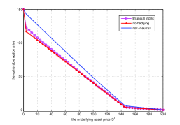
We present results for the European put with payoff . If and are positively correlated, this means when the put option is valuable (in-the-money), the firm’s assets tend to be small, so there is a high risk of default. It is important to take counterparty risk into account for puts in this case, as it will have a relatively large impact on the price. (This would be even more significant when the default trigger involves the option liability). However, for a call, when the call is in-the-money, there is little default risk, and so counterparty risk is less important. Unless otherwise stated, the parameters are: ; ; ; ; ; ; ; ; ; ; ; ; ; ; ; . These parameters result in correlation between the underlying asset and firm’s assets of ; and correlations between each asset and the financial index of .
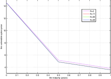
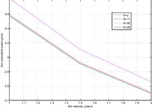
In Figure 1 we show how the approximation converges as we increase the number of time steps . For our parameter values, steps is sufficient for the prices to converge and we use it in all subsequent figures. We aim to compare the utility indifference price with hedging in the financial index with the benchmark risk neutral price in a complete market (computed as in Corollary 2.4 with , as studied in Klein [30]). We also compare to the situation where the financial index is independent of the other assets and thus there is no hedging carried out. This price has an explicit formula:
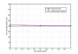
Figure 2 provides a demonstration of the accuracy of the algorithm. We take and compare the splitting approximation to the above formula.
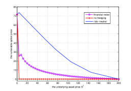
Figure 3 shows the vulnerable option price(s) against the underlying asset price . The two panels of Figure 3 are intended to illustrate a “close or likely to default” scenario (the left panel with relative to ) and a “far or unlikely to default” scenario (the right panel with relative to ). In both panels the risk neutral or complete market price is the highest. As the underlying asset price becomes very large, all option prices tend to zero, as the put is worthless, regardless of the default risk. At , in the right panel, the option price is equal to the option strike . In the left panel, the option price is lower due to the risk of counterparty default. As increases, all option prices decrease, as the moneyness of the put changes. When is close to zero, we see a dramatic drop in the utility indifference prices (relative to the risk neutral prices) due to the risk aversion towards unhedgeable price and default risks. Recall that since the underlying asset and firm’s assets are positively correlated, default risk becomes more important for low values of the underlying asset. The price drop is much more significant in the left panel (and in this extreme case, the option price drops down to zero if no hedging can be carried out), where the likelihood of counterparty default is higher. The option holder’s risk aversion causes the utility indifference prices to lie below the risk neutral price (in each default scenario) with the relative discount to the risk neutral price being much greater in the left panel where default is more likely. Assuming the holder can hedge in the financial index, there is a drop of around 75% from the risk-neutral price to the utility indifference price. In the right panel, where the likelihood of default is relatively low, the difference between the utility indifference price(s) and the risk-neutral price is not as dramatic, and is at most around 20% of the risk-neutral price. We also see that the ability to hedge in the correlated financial index (versus no hedging at all) is more important when the default risk is higher (in the left panel).
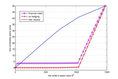
Figure 4 displays the impact of the option writer’s asset value on the option price for a fixed asset price . We see a dramatic difference in the behavior of the risk neutral price and the utility indifference prices. Under risk neutrality, the option price increases smoothly with . However, under utility indifference, the prices are low and do not change much with values of below the default trigger of . This is despite the put being in-the-money. As increases beyond the default level, the likelihood of default diminishes, and the utility indifference prices start to increase with . Note that the utility price is not always below the risk neutral price. Although Proposition 2.5 tells us that the risk neutral price is obtained as a limiting case of the utility indifference price, it requires condition (2.17) to hold.
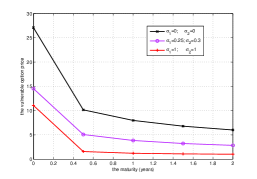
Figure 5 compares how the vulnerable option price changes with risk aversion parameter , and the idiosyncratic volatilities . The left panel plots vulnerable option prices against maturity for various values of risk aversion . We see that the more risk averse the option holder is, the less she will pay for the option, consistent with Proposition 2.6. The other observation is that option prices for a fixed are decreasing with maturity . The risk neutral price is also decreasing with , albeit very gradually. This is in contrast to risk neutral prices for non-default European put options which will increase in provided there are no dividends. The reason is that there is a tradeoff between price and default risk. If the maturity is longer, there is more chance for both and to fall - falling means the put is more valuable, but falling increases the default risk. For the parameters considered, the default risk is the dominant factor and thus the option price decreases with . This is also in contrast to the call option, where Klein [30] reports that the risk neutral price increases with maturity.
Recall that we do not expect price monotonicity in terms of the correlations, except in the situation outlined in Proposition 2.6. Here we give an example of prices for various values of the idiosyncratic volatilities . The left panel sets parameters to be and to satisfy the CAPM restriction on Sharpe ratios. If , then we have , and . Similarly if and then , and . Finally, if then , and . We see that as increase, the utility indifference price falls. Correspondingly, as the correlations increase, the option price rises.
Appendix A Proof of Theorem 2.3
A.1 Derivation of Pricing PDE (2.12)
The proof is an extension of Theorem 2.3 of Henderson and Liang [24], where we considered the special case in a non-Markovian setting. We first transform the optimal portfolio problem (2.4) into a risk-sensitive control formulation, and derive a quadratic BSDE representation for its value process and the associated optimal trading strategy. The problem (2.4) can be reformulated as
For any , by using the distribution property of the random time (see Chapter 8 of Bielecki and Rutkowski [7] for example), we calculate the above conditional expectation, which is with
Therefore, in order to solve the optimal portfolio problem (2.4), we only need to solve the following risk-sensitive control problem:
| (A.1) |
and then the value process of (2.4) is given by
| (A.2) |
In the following, we will first work out the BSDE representation for , and then obtain the BSDE representation for by the comparison principle. For any , we change the probability measure from to by defining
where is the Doléans-Dade exponential. By Girsanov’s theorem, is the Brownian motion under the new probability measure . With the new Brownian motion , the logarithm price processes of the non-traded assets satisfy
| (A.3) |
and becomes
with the stochastic discount factor :
By the martingale representation theorem, there exists an -valued predictable process such that
| (A.4) |
From (A.1), . Itô’s formula then implies that
| (A.5) |
where . Equivalently, under the original probability measure , we write
| (A.6) |
We notice that (A.1) is a quadratic BSDE with bounded terminal data and coefficients, whose existence and uniqueness is guaranteed by Theorems 2.3 and 2.6 of Kobylanski [32]. Moreover, the comparison principle holds for (A.1). Let such that
for . Then .
We claim that the value process of our risk-sensitive control problem (A.1) is given by the solution of the following quadratic BSDE:
| (A.7) |
with the associated optimal portfolio:
Indeed, by Theorems 2.3 and 2.6 of Kobylanski [32], the quadratic BSDE (A.1) admits a unique bounded solution with its martingale representation part . To prove the claim, we notice that for any ,
and for , the equality holds:
Then the claim follows from the comparison principle for (A.1).
The optimization problem (2.5) is a special case of (2.4) with , whose value process is given by and the optimal control on the event is given by .
By Definition 2.2, the utility indifference price is such that
from which we obtain
The hedging strategy on the event is given as .
A.2 Well posedness of the Pricing PDE (2.12)
The existence and uniqueness of bounded solutions to (2.12) are easily obtained from [32]. We next derive explicit bounds for the solution , which are used in Proposition 2.6.
It is obvious that the solution is nonnegative: . Let be the solution of the pricing PDE with the full recovery , so it satisfies the following PDE with quadratic gradients:
| (A.10) |
Note that , since
so that is a supersolution to (2.12). On the other hand, is the (sub)solution to (2.12), and . By the comparison principle, we conclude that on .
The solution to PDE (A.10) is interpreted as the utility indifference price without intertemporal default, and we claim that is bounded from above by , which is the solution to PDE (A.10) with , that is, satisfies the following linear PDE:
| (A.13) |
Indeed, note that , since the terms involving in can be regrouped as (omitting the arguments in and )
so that is a supersolution to (A.10). On the other hand, is the (sub)solution to (A.10), and . The comparison principle implies that on .
It is well known that the linear PDE (A.13) admits a unique bounded solution since the terminal data is bounded. Hence, there exists a constant such that
Finally, we show that is Lipschitz continuous in . This in turn gives us the uniform boundedness of and therefore the hedging strategy . Indeed, since is bounded and , is Lipschitz continuous in . On the other hand, has at most quadratic growth in gradients. We can apply Theorem 2.9 of Delarue [15] to conclude that the solution indeed has bounded gradients: is uniformly bounded.
References
- [1] Barles, G., The convergence of approximation schemes for parabolic equations arising in finance theory, Numerical methods in finance, edited by L. C. G. Rogers and D. Talay, Cambridge University Press, (1997), 1–21.
- [2] Barles, G. and E. R. Jakobsen, Error bounds for monotone approximation schemes for parabolic Hamilton-Jacobi-Bellman equations, Mathematics of Computation, 76, (2007), 1861–1893.
- [3] Barles, G. and P. E. Souganidis, Convergence of approximation schemes for fully nonlinear second order equations, Asymptotic Analysis, 4(3), (1991), 271–283.
- [4] Becherer, D., Rational hedging and valuation of integrated risks under constant absolute risk aversion, Insurance: Mathematics and Economics, 33(1), (2003), 1–28.
- [5] Bielecki, T. R., Crepey, S., Jeanblanc, M. and B. Zagari, Valuation and hedging of CDS counterparty exposure in a markov copula model, International Journal of Theoretical and Applied Finance, 15(1), (2012), 1–39.
- [6] Bielecki, T. R. and M. Jeanblanc, Indifference pricing of defaultable claims, Indifference Pricing, edited by R. Carmona, Princeton University Press, (2009), 211–240.
- [7] Bielecki, T. R. and M. Rutkowski, Credit risk: Modelling, valuation and hedging, Springer Finance. Springer-Verlag, Berlin, (2002).
- [8] Blanchet-Scalliet, C., El Karoui, N., Jeanblanc, M. and L. Martellini, Optimal investment decisions when time-horizon is uncertain, Journal of Mathematical Economics, 44(11), (2008), 1100–1113.
- [9] Brigo, D., Capponi, A. and A. Pallavicini, Arbitrage-free bilateral counterparty risk valuation under collateralization and application to credit default swaps, Mathematical Finance, 24, (2014), 125–146.
- [10] Carmona, R. (editor), Indifference pricing, theory and applications, Princeton University Press, (2009).
- [11] Carmona, R. and M. Ludkovski, Indifference pricing of commodity forwards with partial observations and basis risk, Permanent Working Paper, (2006).
- [12] Crépey, S., Bilateral counterparty risk under funding constraints part I: Pricing, Math. Finance., to appear.
- [13] Crépey, S., Bilateral counterparty risk under funding constraints part II: CVA, Math. Finance., to appear.
- [14] Davis, M. H. A., Optimal hedging with basis risk, Second Bachelier Colloquium on Stochastic Calculus and Probability, edited by Y. Kabanov, R. Lipster, and J. Stoyanov, Springer, (2006), 169–187.
- [15] Delarue, F., Estimates of the solutions of a system of quasi-linear PDEs: a probabilistic scheme, Séminaire de Probabilités XXXVII, Lecture Notes in Math., Spring, 1832, (2003), 290–332.
- [16] Frei, C. and M. Schweizer, Exponential utility indifference valuation in two Brownian settings with stochastic correlation, Advances in Applied Probability, 40, (2008), 401–423.
- [17] Frei, C. and M. Schweizer, Exponential Utility Indifference Valuation in a General Semimartingale Model, Optimality and Risk: Modern Trends in Mathematical Finance, edited by F. Delbaen, M. Rásonyi and C. Stricker, Springer, (2009), 49-86.
- [18] Halperin, I. and A. Itkin, Pricing illiquid options with liquid proxies using mixed-dynamic static hedging, International Journal of Theoretical and Applied Finance, 16, 7, (2013).
- [19] Halperin, I. and A. Itkin, Pricing options on illiquid assets with liquid proxies using utility indifference and dynamic-static hedging, Quantitative Finance, 14, 3, (2014), 427-442.
- [20] Henderson, V., Valuation of claims on nontraded assets using utility maximization, Mathematical Finance, 12, (2002), 351–373.
- [21] Henderson, V., The impact of the market portfolio on the valuation, incentives and optimality of executive stock options, Quantitative Finance, 5(1), (2005), 1–13.
- [22] Henderson, V. and D. Hobson, Substitute hedging, RISK, 15(5), (2002), 71–75. (Reprinted in Exotic Options: The Cutting Edge Collection, RISK Books, London, 2003.)
- [23] Henderson, V. and D. Hobson, Utility indifference pricing: an overview, Indifference Pricing, edited by R. Carmona, Princeton University Press, (2009), 44–74.
- [24] Henderson, V. and G. Liang, Pseudo linear pricing rule for utility indifference valuation, Finance and Stochastics, 18(3), (2014), 593–615.
- [25] Jaimungal, S. and G. Sigloch, Incorporating risk and ambiguity aversion into a hybrid model of default, Mathematical Finance, 22(1), (2012), 57–81.
- [26] Jakobsen, E. R., On the rate of convergence of approximation schemes for Bellman equations associated with optimal stopping time problems, Math. Models Methods Appl. Sci., 13(5), (2003), 613-644.
- [27] Jiao, Y. and H. Pham, Optimal investment with counterparty risk: a default-density modeling approach, Finance and Stochastics, 15(4), (2011), 725–753.
- [28] Jiao, Y., Kharroubi, I. and H. Pham, Optimal investment under multiple defaults risk: a BSDE-decomposition approach, Annals of Applied Probability, 23(2), (2013), 427–857.
- [29] Johnson, H. and R. Stulz, The pricing of options with default risk, Journal of Finance, 42, (1987), 267–280.
- [30] Klein, P., Pricing Black-Scholes options with correlated credit risk, Journal of Banking and Finance, 20, (1996), 1211–1229.
- [31] Klein, P. and M. Inglis, Pricing vulnerable European options when the option’s payoff can increase the risk of financial distress, Journal of Banking and Finance, 25, (2001), 993–1012.
- [32] Kobylanski, M., Backward stochastic differential equations and partial differential equations with quadratic growth, Annals of Probability 28 (2000) 558–602.
- [33] Kramkov, D. and M. Sirbu, Asymptotic analysis of utility-based hedging strategies for small number of contingent claims, Stochastic Processes and Their Applications, 117(11), (2007), 1606-1620.
- [34] Krylov, N. V., On the rate of convergence of finite-difference approximations for Bellman’s equations with variable coefficients, Probability Theory and Related Fields 117(1), (2000), 1–16.
- [35] Leung, T., S. Sircar and T. Zariphopoulou, Credit derivatives and risk aversion, Advances in Econometrics, edited by T. Fomby, J.-P. Fouque and K. Solna, Elsevier Science, 22, (2008), 275–291.
- [36] Liang, G. and L. Jiang, A modified structural model for credit risk, IMA Journal of Management Mathematics, 23(2), (2012), 147–170.
- [37] Liang, G. and X. Ren, The credit risk and pricing of OTC options, Asia-Pacific Financial Markets, 14(1), (2007), 45–68.
- [38] Marchuk, G. I., Some application of splitting-up methods to the solution of mathematical physics problems, Aplikace Matematiky, 13, (1968), 103–132.
- [39] Monoyios, M., Malliavin calculus method for asymptotic expansion of dual control problems, SIAM J. Finan. Math., 4 (2013), 884–915.
- [40] Musiela, M. and T. Zariphopoulou, An example of indifference prices under exponential preferences, Finance and Stochastics, 8, (2004), 229–239.
- [41] Nadtochiy, S. and T. Zariphopoulou, An approximation scheme for the solution to the optimal investment problem in incomplete markets, SIAM J. Finan. Math., 4(1), (2013), 494–538.
- [42] Sircar, R. and T. Zariphopoulou, Bounds and asymptotic approximations for utility prices when volatility is random, SIAM Journal on Control and Optimization, 43(4), (2005), 1328–1353.
- [43] Sircar, R. and T. Zariphopoulou, Utility valuation of multi-name credit derivatives and application to CDOs, Quantitative Finance, 10(2), (2010), 195–208.
- [44] Tan X., A splitting method for fully nonlinear degenerate parabolic PDEs, Electron. J. Probab., 18(15), (2013), 1-24.
- [45] Tehranchi, M., Explicit solutions of some utility maximization problems in incomplete markets, Stochastic Processes and Their Applications, 114(1), (2004), 109–125.
- [46] Tourin, A., Splitting methods for Hamilton-Jacobi equations, Numer. Methods Partial Differential Equations, 22(2), (2006), 381–396.
- [47] Zhou, T., Indifference valuation of mortgage-backed securities in the presence of prepayment risk, Mathematical Finance, 20, (2010), 479–507.