No Free Lunch versus Occam’s Razor in Supervised Learning
 

Abstract

The No Free Lunch theorems are often used to argue that domain specific knowledge is required to design successful algorithms. We use algorithmic information theory to argue the case for a universal bias allowing an algorithm to succeed in all interesting problem domains. Additionally, we give a new algorithm for off-line classification, inspired by Solomonoff induction, with good performance on all structured (compressible) problems under reasonable assumptions. This includes a proof of the efficacy of the well-known heuristic of randomly selecting training data in the hope of reducing the misclassification rate.

Contents

1. 1 Introduction
2. 2 Preliminaries
3. 3 No Free Lunch Theorem
4. 4 Complexity-based classification
5. 5 Discussion
6. A Technical proofs

Keywords

Supervised learning; Kolmogorov complexity; no free lunch; Occam’s razor.

1 Introduction

The No Free Lunch (NFL) theorems, stated and proven in various settings and domains [Sch94, Wol01, WM97], show that no algorithm performs better than any other when their performance is averaged uniformly over all possible problems of a particular type. These are often cited to argue that algorithms must be designed for a particular domain or style of problem, and that there is no such thing as a general purpose algorithm.

On the other hand, Solomonoff induction [Sol64a, Sol64b] and the more general AIXI model [Hut04] appear to universally solve the sequence prediction and reinforcement learning problems respectively. The key to the apparent contradiction is that Solomonoff induction and AIXI do not assume that each problem is equally likely. Instead they apply a bias towards more structured problems. This bias is universal in the sense that no class of structured problems is favored over another. This approach is philosophically well justified by Occam’s razor.

The two classic domains for NFL theorems are optimisation and classification. In this paper we will examine classification and only remark that the case for optimisation is more complex. This difference is due to the active nature of optimisation where actions affect future observations.

Previously, some authors have argued that the NFL theorems do not disprove the existence of universal algorithms for two reasons.

1. That taking a uniform average is not philosophically the right thing to do, as argued informally in [GCP05].

2. Carroll and Seppi in [CS07] note that the NFL theorem measures performance as misclassification rate, where as in practise, the utility of a misclassification in one direction may be more costly than another.

We restrict our consideration to the task of minimising the misclassification rate while arguing more formally for a non-uniform prior inspired by Occam’s razor and formalised by Kolmogorov complexity. We also show that there exist algorithms (unfortunately only computable in the limit) with very good properties on all structured classification problems.

The paper is structured as follows. First, the required notation is introduced (Section 2). We then state the original NFL theorem, give a brief introduction to Kolmogorov complexity, and show that if a non-uniform prior inspired by Occam’s razor is used, then there exists a free lunch (Section 3). Finally, we give a new algorithm inspired by Solomonoff induction with very attractive properties in the classification problem (Section 4).

2 Preliminaries

Here we introduce the required notation and define the problem setup for the No Free Lunch theorems.

Strings. A finite string $x$ over alphabet $X$ is a finite sequence $x_{1}x_{2}x_{3}\cdots x_{n-1}x_{n}$ with $x_{i}\in X$. An infinite string $x$ over alphabet $X$ is an infinite sequence $x_{1}x_{2}x_{3}\cdots$. Alphabets are usually countable or finite, while in this paper they will almost always be binary. For finite strings we have a length function defined by $\ell(x):=n$ for $x=x_{1}x_{2}\cdots x_{n}$. The empty string of length $0$ is denoted by $\epsilon$. The set $X^{n}$ is the set of all strings of length $n$. The set $X^{*}$ is the set of all finite strings. The set $X^{\infty}$ is the set of all infinite strings. Let $x$ be a string (finite or infinite) then substrings are denoted $x_{s:t}:=x_{s}x_{s+1}\cdots x_{t-1}x_{t}$ where $s\leq t$. A useful shorthand is $x_{<t}:=x_{1:t-1}$. Let $x,y\in X^{*}$ and $z\in X^{\infty}$ with $\ell(x)=n$ and $\ell(y)=m$ then

$$xy :=x_{1}x_{2},\cdots x_{n-1}x_{n}y_{1}y_{2}\cdots y_{m-1}y_{m}$$

$$xz :=x_{1}x_{2},\cdots x_{n-1}x_{n}z_{1}z_{2}z_{3}\cdots$$

As expected, $xy$ is finite and has length $\ell(xy)=n+m$ while $xz$ is infinite. For binary strings, we write $\#1(x)$ and $\#0(x)$ to mean the number of 0’s and number of 1’s in $x$ respectively.

Classification. Informally, a classification problem is the task of matching features to class labels. For example, recognizing handwriting where the features are images and the class labels are letters. In supervised learning, it is (usually) unreasonable to expect this to be possible without any examples of correct classifications. This can be solved by providing a list of feature/class label pairs representing the true classification of each feature. It is hoped that these examples can be used to generalize and correctly classify other features.

The following definitions formalize classification problems, algorithms capable of solving them, as well as the loss incurred by an algorithm when applied to a problem, or set of problems. The setting is that of transductive learning as in [DEyM04].

Definition 1 (Classification Problem).

Let $X$ and ${Y}$ be finite sets representing the feature space and class labels respectively. A classification problem over $X,{Y}$ is defined by a function $f:X\to{Y}$ where $f(x)$ is the true class label of feature $x$.

In the handwriting example, $X$ might be the set of all images of a particular size and ${Y}$ would be the set of letters/numbers as well as a special symbol for images that correspond to no letter/number.

Definition 2 (Classification Algorithm).

Let $f$ be a classification problem and ${X_{m}}\subseteq X$ be the training features on which $f$ will be known. We write $f_{X_{m}}$ to represent the function $f_{X_{m}}:{X_{m}}\to{Y}$ with $f_{X_{m}}(x):=f(x)$ for all $x\in{X_{m}}$. A classification algorithm is a function, $A$, where $A(f_{X_{m}},x)$ is its guess for the class label of feature $x\in{X_{u}}:=X-{X_{m}}$ when given training data $f_{X_{m}}$. Note we implicitly assume that $X$ and ${Y}$ are known to the algorithm.

Definition 3 (Loss function).

The loss of algorithm $A$, when applied to classification problem $f$, with training data ${X_{m}}$ is measured by counting the proportion of misclassifications in the testing data, ${X_{u}}$.

$$L_{A}(f,{X_{m}}):={1\over|{X_{u}}|}\sum_{x\in{X_{u}}}[\![A(f_{X_{m}},x)\neq f(x)]\!]$$

where $[\![]\!]$ is the indicator function defined by, $[\![expr]\!]=1$ if $expr$ is true and $0$ otherwise.

We are interested in the expected loss of an algorithm on the set of all problems where expectation is taken with respect to some distribution $P$.

Definition 4 (Expected loss).

Let $\mathcal{M}$ be the set of all functions from $X$ to ${Y}$ and $P$ be a probability distribution on $\mathcal{M}$. If ${X_{m}}$ is the training data then the expected loss of algorithm $A$ is

$$L_{A}(P,{X_{m}}):=\sum_{f\in\mathcal{M}}P(f)L_{A}(f,{X_{m}})$$

3 No Free Lunch Theorem

We now use the above notation to give a version of the No Free Lunch Theorem of which Wolpert’s is a generalization.

Theorem 5 (No Free Lunch).

Let $P$ be the uniform distribution on $\mathcal{M}$. Then the following holds for any algorithm $A$ and training data ${X_{m}}\subseteq X$.

$$L_{A}(P,{X_{m}})=|{Y}-1|/|{Y}|$$ (1)

The key to the proof is the following observation. Let $x\in{X_{u}}$, then for all $y\in{Y}$, $P(f(x)=y|f|_{X_{m}})=P(f(x)=y)=1/|{Y}|$. This means no information can be inferred from the training data, which suggests no algorithm can be better than random.

Occam’s razor/Kolmogorov complexity. The theorem above is often used to argue that no general purpose algorithm exists and that focus should be placed on learning in specific domains.

The problem with the result is the underlying assumption that $P$ is uniform, which implies that training data provides no evidence about the true class labels of the test data. For example, if we have classified the sky as blue for the last 1,000 years then a uniform assumption on the possible sky colours over time would indicate that it is just as likely to be green tomorrow as blue, a result that goes against all our intuition.

How then, do we choose a more reasonable prior? Fortunately, this question has already been answered heuristically by experimental scientists who must endlessly choose between one of a number of competing hypotheses. Given any experiment, it is easy to construct a hypothesis that fits the data by using a lookup table. However such hypotheses tend to have poor predictive power compared to a simple alternative that also matches the data. This is known as the principle of parsimony, or Occam’s razor, and suggests that simple hypotheses should be given a greater weight than more complex ones.

Until recently, Occam’s razor was only an informal heuristic. This changed when Solomonoff, Kolmogorov and Chaitin independently developed the field of algorithmic information theory that allows for a formal definition of Occam’s razor. We give a brief overview here, while a more detailed introduction can be found in [LV08]. An in depth study of the philosophy behind Occam’s razor and its formalisation by Kolmogorov complexity can be found in [KLV97, RH11]. While we believe Kolmogorov complexity is the most foundational formalisation of Occam’s razor, there have been other approaches such as MML [WB68] and MDL [Grü07]. These other techniques have the advantage of being computable (given a computable prior) and so lend themselves to good practical applications.

The idea of Kolmogorov complexity is to assign to each binary string an integer valued complexity that represents the length of its shortest description. Those strings with short descriptions are considered simple, while strings with long descriptions are complex. For example, the string consisting of 1,000,000 1’s can easily be described as “one million ones”. On the other hand, to describe a string generated by tossing a coin 1,000,000 times would likely require a description about 1,000,000 bits long. The key to formalising this intuition is to choose a universal Turing machine as the language of descriptions.

Definition 6 (Kolmogorov Complexity).

Let $U$ be a universal Turing machine and $x\in\mathcal{B}^{*}$ be a finite binary string. Then define the plain Kolmogorov complexity $C(x)$ to be the length of the shortest program (description) $p$ such that $U(p)=x$.

$$C(x):=\min_{p\in\mathcal{B}^{*}}\left\{\ell(p):U(p)=x\right\}$$

It is easy to show that $C$ depends on choice of universal Turing machine $U$ only up to a constant independent of $x$ and so it is standard to choose an arbitrary reference universal Turing machine.

For technical reasons it is difficult to use $C$ as a prior, so Solomonoff introduced monotone machines to construct the Solomonoff prior, $\mathbf{M}$. A monotone Turing machine has one read-only input tape which may only be read from left to right and one write-only output tape that may only be written to from left to right. It has any number of working tapes. Let $T$ be such a machine and write $T(p)=x$ to mean that after reading $p$, $x$ is on the output tape. The machines are called monotone because if $p$ is a prefix of $q$ then $T(p)$ is a prefix of $T(q)$. It is possible to show there exists a universal monotone Turing machine $U$ and this is used to define monotone complexity $Km$ and Solomonoff’s prior, $\mathbf{M}$.

Definition 7 (Monotone Complexity).

Let $U$ be the reference universal monotone Turing machine then define $Km$, $\mathbf{M}$ and $K\!M$ as follows,

$$Km(x) :=\min\left\{\ell(p):U(p)=x*\right\}$$

$$\mathbf{M}(x) :=\sum_{U(p)=x*}2^{-\ell(p)}$$

$$K\!M(x) :=-\log\mathbf{M}(x)$$

where $U(p)=x*$ means that when given input $p$, $U$ outputs $x$ possibly followed by more bits.

Some facts/notes follow.

1. For any $n$, $\sum_{x\in\mathcal{B}^{n}}\mathbf{M}(x)\leq 1$.

2. $Km$, $\mathbf{M}$ and $K\!M$ are incomputable.

3. $0<K\!M(x)\approx Km(x)\approx C(x)<\ell(x)+O(1)$

To illustrate why $\mathbf{M}$ gives greater weight to simple $x$, suppose $x$ is simple then there exists a relatively short monotone Turing machine $p$, computing it. Therefore $Km(x)$ is small and so $2^{-Km(x)}\approx\mathbf{M}(x)$ is relatively large.

Since $\mathbf{M}$ is a semi-measure rather than a proper measure, it is not appropriate to use it in place of $P$ when computing expected loss. However it can be normalized to a proper measure, $\mathbf{M}_{norm}$ defined inductively by

$$\mathbf{M}_{norm}(\epsilon) :=1 \mathbf{M}_{norm}(xb) :=\mathbf{M}_{norm}(x){\mathbf{M}(xb)\over\mathbf{M}(x0)+\mathbf{M}(x1)}$$

Note that this normalisation is not unique, but is philosophically and technically the most attractive and was used and defended by Solomonoff. For a discussion of normalisation, see [LV08, p.303]. The normalised version satisfies $\sum_{x\in\mathcal{B}^{n}}\mathbf{M}_{norm}(x)=1$.

We will also need to define $\mathbf{M}/K\!M$ with side information, $\mathbf{M}(y;x):=\mathbf{M}(y)$ where $x*$ is provided on a spare tape of the universal Turing machine. Now define $K\!M(y;x):=-\log\mathbf{M}(y;x)$. This allows us to define the complexity of a function in terms of its output relative to its input.

Definition 8 (Complexity of a function).

Let $X=\left\{x_{1},\cdots,x_{n}\right\}\subseteq\mathcal{B}^{k}$ and $f:X\to\mathcal{B}$ then define the complexity of $f$, $K\!M(f;X)$ by

$$K\!M(f;X):=K\!M(f(x_{1})f(x_{2})\cdots f(x_{n});x_{1},x_{2},\cdots,x_{n})$$

An example is useful to illustrate why this is a good measure of the complexity of $f$.

Example 9.

Let $X\subseteq\mathcal{B}^{n}$ for some $n$, and ${Y}=\mathcal{B}$ and $f:X\to{Y}$ be defined by $f(x)=[\![x_{n}=1]\!]$. Now for a complex $X$, the string $f(x_{1})f(x_{2})\cdots$ might be difficult to describe, but there is a very short program that can output $f(x_{1})f(x_{2})\cdots$ when given $x_{1}x_{2}\cdots$ as input. This gives the expected result that $K\!M(f;X)$ is very small.

Free lunch using Solomonoff prior. We are now ready to use $\mathbf{M}_{norm}$ as a prior on a problem family. The following proposition shows that when problems are chosen according to the Solomonoff prior that there is a (possibly small) free lunch.

Before the proposition, we remark on problems with maximal complexity, $K\!M(f;X)=O(|X|)$. In this case $f$ exhibits no structure allowing it to be compressed, which turns out to be equivalent to being random in every intuitive sense [ML66]. We do not believe such problems are any more interesting than trying to predict random coin flips. Further, the NFL theorems can be used to show that no algorithm can learn the class of random problems by noting that almost all problems are random. Thus a bias towards random problems is not much of a bias (from uniform) at all, and so at most leads to a decreasingly small free lunch as the number of problems increases.

Proposition 1 (Free lunch under Solomonoff prior).

Let ${Y}=\mathcal{B}$ and fix a $k\in\mathbb{N}$. Now let $X=\mathcal{B}^{n}$ and ${X_{m}}\subset X$ such that $|{X_{m}}|=2^{n}-k$. For sufficiently large $n$ there exists an algorithm $A$ such that

$$L_{A}(\mathbf{M}_{norm},{X_{m}})<1/2$$

Before the proof of Proposition 1, we require an easy lemma.

Lemma 10.

Let $N\subset\mathcal{M}$ then there exists an algorithm $A_{N}$ such that

$$\sum_{f\in N}P(f)L_{A_{N}}(f,{X_{m}})\leq{1\over 2}\sum_{f\in N}P(f)$$

Proof.

Let $A_{i}$ with $i\in\left\{0,1\right\}$ be the algorithm always choosing $i$. Note that

$$\sum_{f\in N}P(f)L_{A_{0}}(f,{X_{m}})=\sum_{f\in N}P(f)(1-L_{A_{1}}(f,{X_{m}}))$$

The result follows easily. ∎

Proof of Proposition 1.

Now let $\mathcal{M}_{1}$ be the set of all $f\in\mathcal{M}$ with $f(y)=1\forall y\in{X_{m}}$ and $\mathcal{M}_{0}=\mathcal{M}-\mathcal{M}_{1}$. Now construct an $A$ by

$$A(f_{X_{m}},x)=\begin{cases}1&\text{if }f\in\mathcal{M}_{1}\\ A_{\mathcal{M}_{0}}(f_{X_{m}},x)&\text{otherwise}\end{cases}$$

Let $f_{1}\in\mathcal{M}_{1}$ be the constant valued function such that $f_{1}(x)=1\forall x$ then

$$L_{A}(\mathbf{M}_{norm},{X_{m}}) =\sum_{f\in\mathcal{M}}\mathbf{M}_{norm}(f)L_{A}(f,{X_{m}})$$ (2)

$$=\sum_{f\in\mathcal{M}_{0}}\mathbf{M}_{norm}(f)L_{A}(f,{X_{m}})+\sum_{f\in\mathcal{M}_{1}}\mathbf{M}_{norm}(f)L_{A}(f,{X_{m}})$$ (3)

$$\leq{1\over 2}\sum_{f\in\mathcal{M}_{0}}\mathbf{M}_{norm}(f)+\sum_{f\in\mathcal{M}_{1}}\mathbf{M}_{norm}(f)L_{A}(f,{X_{m}})$$ (4)

$$\leq{1\over 2}\sum_{f\in\mathcal{M}_{0}}\mathbf{M}_{norm}(f)+\sum_{f\in\mathcal{M}_{1}-f_{1}}\mathbf{M}_{norm}(f)$$ (5)

$$<{1\over 2}(1-\delta)+\sum_{f\in\mathcal{M}_{1}-f_{1}}\mathbf{M}_{norm}(f)<{1\over 2}$$ (6)

where (2) is definitional, (3) follows by splitting the sum into $\mathcal{M}_{0}$ and $\mathcal{M}_{1}$, (4) by the previous lemma, (5) since loss is bounded by $1$ and the loss incurred on $f_{1}$ is $0$. The first inequality of (6) follows since it can be shown that there exists a $\delta>0$ such that $\mathbf{M}_{norm}(f_{1})>\delta$ with $\delta$ independent of $n$. The second because $\max_{f\in\mathcal{M}_{1}-\left\{f_{1}\right\}}\mathbf{M}_{norm}(f)\stackrel{{\scriptstyle n\to\infty}}{{\longrightarrow}}0$ and $|\mathcal{M}_{1}|$ is independent of $n$. ∎

The proposition is unfortunately extremely weak. It is more interesting to know exactly what conditions are required to do much better than random. In the next section we present an algorithm with good performance on all well structured problems when given “good” training data. Without good training data, even assuming a Solomonoff prior, we believe it is unlikely that the best algorithm will perform well.

Note that while it appears intuitively likely that any non-uniform distribution such as $\mathbf{M}_{norm}$ might offer a free lunch, this is in fact not true. It is shown in [SVW01] that there exist non-uniform distributions where the loss over a problem family is independent of algorithm. These distributions satisfy certain symmetry conditions not satisfied by $\mathbf{M}_{norm}$, which allows Proposition 1 to hold.

4 Complexity-based classification

Solomonoff induction is well known to solve the online prediction problem where the true value of each classification is known after each guess. In our setup, the true classification is only known for the training data, after which the algorithm no longer receives feedback. While Solomonoff induction can be used to bound the number of total errors while predicting deterministic sequences, it gives no indication of when these errors may occur. For this reason we present a complexity-inspired algorithm with better properties for the offline classification problem.

Before the algorithm we present a little more notation. As usual, let $X=\left\{x_{1},x_{2},\cdots,x_{n}\right\}\subseteq\mathcal{B}^{k}$, ${Y}=\mathcal{B}$ and let ${X_{m}}\subseteq X$ be the training data. Now define an indicator function $\chi$ by $\chi_{i}:=[\![x_{i}\in{X_{m}}]\!]$.

Definition 11.

Let $f\in{Y}^{X}$ be a classification problem. The algorithm $A^{*}$ is defined in two steps.

$$\tilde{f} :=\operatornamewithlimits{arg\,min}_{\tilde{f}\in{Y}^{X}}\left\{K\!M(\tilde{f};X):\chi_{i}=1\implies\tilde{f}(x_{i})=f(x_{i})\right\}$$

$$A^{*}(f_{X_{m}},x_{i}) :=\tilde{f}(x_{i})$$

Essentially $A^{*}$ chooses for its model the simplest $\tilde{f}$ consistent with the training data and uses this for classifying unseen data. Note that the definition above only uses the value $y_{i}=f(x_{i})$ where $\chi_{i}=1$, and so it does not depend on unseen labels.

If $K\!M(f;X)$ is “small” then the function we wish to learn is simple so we should expect to be able to perform good classification, even given a relatively small amount of training data. This turns out to be true, but only with a good choice of training data. It is well known that training data should be “broad enough”, and this is backed up by the example below and by Theorem 14, which give an excellent justification for random training data based on good theoretical (Theorem 14) and philosophical (AIT) underpinnings. The following example demonstrates the effect of bad training data on the performance of $A^{*}$.

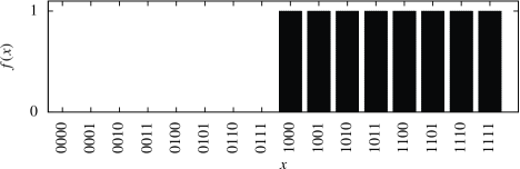
Figure 1: A simple problem

Example 12.

Let $X=\left\{0000,0001,0010,0011,\cdots,1101,1110,1111\right\}$ and $f(x)$ be defined to be the first bit of $x$ as in Figure 1. Now suppose $\chi=1^{8}0^{8}$ (So the algorithm is only allowed to see the true class labels of $x_{1}$ through $x_{8}$). In this case, the simplest $\tilde{f}$ consistent with the first 16 data points, all of which are zeros, is likely to be $\tilde{f}(x)=0$ for all $x\in X$ and so $A^{*}$ will fail on every piece of testing data!

On the other hand, if $\chi=001010011101101$, which was generated by tossing a coin 16 times, then $\tilde{f}$ will very likely be equal to $f$ and so $A^{*}$ will make no errors. Even if $\chi$ is zero about the critical point in the middle ($\chi_{8}=\chi_{9}=0$) then $\tilde{f}$ should still match $f$ mostly around the left and right and will only be unsure near the middle.

Note, the above is not precisely true since for small strings the dependence of $K\!M$ on the universal monotone Turing machine can be fairly large. However if we increase the size of the example so that $|X|>1000$ then these quirks disappear for natural reference universal Turing machines.

Definition 13 (Entropy).

Let $\theta\in[0,1]$

$$H(\theta):=\begin{cases}-[\theta\log\theta+(1-\theta)\log(1-\theta)]&\text{if }\theta\neq 0\text{ and }\theta\neq 1\\ 0&\text{otherwise}\end{cases}$$

Theorem 14.

Let $\theta\in(0,1)$ be the proportion of data to be given for training then:

1. There exists a $\chi\in\mathcal{B}^{\infty}$ (training set) such that for all $n\in\mathbb{N}$, $\theta n-c_{1}<\#1(\chi_{1:n})<\theta n+c_{1}$ and $nH(\theta)-c_{2}<K\!M(\chi_{1:n})$ for some $c_{1},c_{2}\in\mathbb{R}^{+}$.

2. For $n=|X|$, the loss of algorithm $A^{*}$ when using training data determined by $\chi$ is bounded by

   $$L_{A^{*}}(f,{X_{m}})<{2K\!M(f;X)+K\!M(X)+c_{2}+c_{3}\over{n(1-\theta-c_{1}/n)\log(1-\theta+c_{1}/n)^{-1}}}$$

   where $c_{3}$ is some constant independent of all inputs.

This theorem shows that $A^{*}$ will do well on all problems satisfying $K\!M(f;X)=o(n)$ when given good (but not necessarily a lot) of training data. Before the proof, some remarks.

1. The bound is a little messy, but for small $\theta$, large $n$ and simple $X$ we get $L_{A^{*}}(f,{X_{m}})\stackrel{{\scriptstyle\approx}}{{<}}{2K\!M(f;X)/(n\theta)}$.

2. The loss bound is extremely bad for large $\theta$. We consider this unimportant since we only really care if $\theta$ is small. Also, note that if $\theta$ is large then the number of points we have to classify is small and so we still make only a few mistakes.

3. The constants $c_{1},c_{2}$ and $c_{3}$ are relatively small (around 100-500). They represent the length of the shortest programs computing simple transformations or encodings. This is dependent on the universal Turing machine used to define the Solomonoff distribution, but for a natural universal Turing machine we expect it to be fairly small [Hut04, sec.2.2.2].

4. The “special” $\chi$ is not actually that special at all. In fact, it can be generated easily with probability 1 by tossing a coin with bias $\theta$ infinitely often. More formally, it is a $\mu$ Martin-Löf random string where $\mu(1|x)=\theta$ for all $x$. Such strings form a $\mu$-measure 1 set in $\mathcal{B}^{\infty}$.

Proof of Theorem 14.

The first is a basic result in algorithmic information theory [LV08, p.318]. Essentially choosing $\chi$ to be Martin-Löf random with respect to a Bernoulli process parameterized by $\theta$. From now on, let $\bar{\theta}=\#1(\chi)/n$. For simplicity we write $x:=x_{1}x_{2}\cdots x_{n}$, $y:=f(x_{1})f(x_{2})\cdots f(x_{n})$, and $\tilde{y}:=\tilde{f}(x_{1})\tilde{f}(x_{2})\cdots\tilde{f}(x_{n})$. Define indicator $\psi$ by $\psi_{i}:=[\![\chi_{i}=0\wedge y_{i}=\tilde{y}_{i}]\!]$. Now note that there exists $c_{3}\in\mathbb{R}$ such that

$$K\!M(\chi_{1:n})<K\!M(\psi_{1:n};y,\tilde{y})+K\!M(y;x)+K\!M(\tilde{y};x)+K\!M(x)+c_{3}$$ (7)

This follows since we can easily use $y$, $\tilde{y}$ and $\psi_{1:n}$ to recover $\chi_{1:n}$ by $\chi_{i}=1$ if and only if $y_{i}=\tilde{y}_{i}$ and $\psi_{i}\neq 1$. The constant $c_{3}$ is the length of the reconstruction program. Now $K\!M(\tilde{y};x)\leq K\!M(y;x)$ follows directly from the definition of $\tilde{f}$. We now compute an upper bound on $K\!M(\psi)$. Let $\alpha:=L_{A^{*}}(f,{X_{m}})$ be the proportion of the testing data on which $A^{*}$ makes an error. The following is easy to verify:

1. $\#1(\psi)=(1-\alpha)(1-\bar{\theta})n$

2. $\#0(\psi)=(1-(1-\alpha)(1-\bar{\theta}))n$

3. $y_{i}\neq\tilde{y}_{i}\implies\psi_{i}=0$

4. $\#1(y\oplus\tilde{y})=\alpha(1-\bar{\theta})n$ where $\oplus$ is the exclusive or function.

We can use point 3 above to trivially encode $\psi_{i}$ when $\tilde{y}_{i}\neq y_{i}$. Aside from these, there are exactly $\bar{\theta}n$ 0’s and $(1-\alpha)(1-\bar{\theta})n$ 1’s. Coding this subsequence using frequency estimation gives a code for $\psi_{1:n}$ given $y$ and $\tilde{y}$, which we substitute into (7).

$$nH(\bar{\theta})-c_{2} \leq K\!M(\chi_{1:n})\leq K\!M(\psi_{1:n};y,\tilde{y})+K\!M(y;x)+K\!M(\tilde{y};x)$$

$$\qquad+K\!M(x)+c_{3}$$ (8)

$$\leq 2K\!M(y;x)+K\!M(x)+nJ(\bar{\theta},\alpha)+c_{3}$$

where $J(\bar{\theta},\alpha):=\left[\bar{\theta}+(1-\bar{\theta})(1-\alpha)\right]H\left({\bar{\theta}/\left[\bar{\theta}+(1-\bar{\theta})(1-\alpha)\right]}\right)$. An easy technical result (Lemma 16 in the appendix) shows that for $\bar{\theta}\in(0,1)$

$$0\leq\alpha(1-\bar{\theta})\log{1\over 1-\bar{\theta}}\leq H(\bar{\theta})-J(\bar{\theta},\alpha)$$

Therefore $n\alpha(1-\bar{\theta})\log{1\over 1-\bar{\theta}}\leq 2K\!M(y;x)+K\!M(x)+c_{2}+c_{3}$. The result follows by rearranging and using part 1 of the theorem. ∎

Since the features are known, it is unexpected for the bound to depend on their complexity, $K\!M(X)$. Therefore it is not surprising that this dependence can be removed at a small cost, and with a little extra effort.

Theorem 15.

Under the same conditions as Theorem 14, the loss of $A^{*}$ is bounded by

$$L_{A^{*}}(f,{X_{m}})<{2K\!M(f;X)+2\left[\log|X|+\log\log|X|\right]+c\over{n(1-\theta-c_{1}/n)\log(1-\theta+c_{1}/n)^{-1}}}$$

where $c$ is some constant independent of inputs.

This version will be preferred to Theorem 14 in cases where $K\!M(X)>2\left[\log|X|+\log\log|X|\right]$. The proof of Theorem 15 is almost identical to that of Theorem 14.
Proof sketch: The idea is to replace equation (7) by

$$K\!M(\chi_{1:n},x)<K\!M(\psi_{1:n};y,\tilde{y})+K\!M(y;x)+K\!M(\tilde{y};x)+K\!M(x)+c_{3}$$ (9)

Then use the following identities $K(\chi_{1:n};x,K(x))+K(x)<K(\chi_{1:n},x)-K(\ell(x))<K\!M(\chi_{1:n},x)$ where the inequalities are true up to constants independent of $x$ and $\chi$. Next a counting argument in combination with Stirling’s approximation can be used to show that for most $\chi$ satisfying the conditions in Theorem 14 have $K\!M(\chi_{1:n})<K(\chi_{1:n})<K(\chi_{1:n};x,K(x))+\log\ell(x)+r$ for some constant $r>0$ independent of $x$ and $\chi$. Finally use $K\!M(x)<K(x)$ for all $x$ and $K(\ell(x))<\log\ell(x)+2\log\log\ell(x)+r$ for some constant $r>0$ independent of $x$ to rearrange (9) into

$$K\!M(\chi_{1:n}) <K\!M(\psi_{1:n};y,\tilde{y})+K\!M(y;x)+K\!M(\tilde{y};x)+2\log\ell(x)$$

$$\qquad+2\log\log\ell(x)+c$$

for some constant $c>0$ independent of $\chi,\psi,x$ and $y$. Finally use the techniques in the proof of Theorem 14 to complete the proof. ∎

5 Discussion

Summary. Proposition 1 shows that if problems are distributed according to their complexity, as Occam’s razor suggests they should, then a (possibly small) free lunch exists. While the assumption of simplicity still represents a bias towards certain problems, it is a universal one in the sense that no style of structured problem is more favoured than another.

In Section 4 we gave a complexity-based classification algorithm and proved the following properties:

1. It performs well on problems that exhibit some compressible structure, $K\!M(f;X)=o(n)$.

2. Increasing the amount of training data decreases the error.

3. It performs better when given a good (broad/randomized) selection of training data.

Theorem 14 is reminiscent of the transductive learning bounds of Vapnik and others [DEyM04, Vap82, Vap00], but holds for all Martin-Löf random training data, rather than with high probability. This is different to the predictive result in Solomonoff induction where results hold with probability 1 rather than for all Martin-Löf random sequences [HM07]. If we assume the training set is sampled randomly, then our bounds are comparable to those in [DEyM04].

Unfortunately, the algorithm of Section 4 is incomputable. However Kolmogorov complexity can be approximated via standard compression algorithms, which may allow for a computable approximation of the classifier of Section 4. Such approximations have had some success in other areas of AI, including general reinforcement learning [VNH⁺11] and unsupervised clustering [CV05].

Occam’s razor is often thought of as the principle of choosing the simplest hypothesis matching your data. Our definition of simplest is the hypothesis that minimises $K\!M(f;X)$ (maximises $M(f;X)$). This is perhaps not entirely natural from the informal statement of Occam’s razor, since $M(x)$ contains contributions from all programs computing $x$, not just the shortest. We justify this by combining Occam’s razor with Epicurus principle of multiple explanations that argues for all consistent hypotheses to be considered. In some ways this is the most natural interpretation as no scientist would entirely rule out a hypothesis just because it is slightly more complex than the simplest. A more general discussion of this issue can be found in [Dow11, sec.4]. Additionally, we can argue mathematically that since $K\!M\approx Km$, the simplest hypothesis is very close to the mixture. Therefore the debate is more philosophical than practical in this setting.

An alternative approach to formalising Occam’s razor has been considered in MML [WB68]. However, in the deterministic setting the probability of the data given the hypothesis satisfies $P(D|H)=1$. This means the two part code reduces to the code-length of the prior, $\log(1/P(H))$. This means the hypothesis with minimum message length depends only on the choice of prior, not the complexity of coding the data. The question then is how to choose the prior, on which MML gives no general guidance. Some discussion of Occam’s razor from a Kolmogorov complexity viewpoint can be found in [Hut10, KLV97, RH11], while the relation between MML and Kolmogorov complexity is explored in [WD99].

Assumptions. We assumed finite $X$, ${Y}$, and deterministic $f$, which is the standard transductive learning setting. Generalisations to countable spaces may still be possible using complexity approaches, but non-computable real numbers prove more difficult. One can either argue by the strong Church-Turing thesis that non-computable reals do not exist, or approximate them arbitrarily well. Stochastic $f$ are interesting and we believe a complexity-based approach will still be effective, although the theorems and proofs may turn out to be somewhat different.

Acknowledgements. We thank Wen Shao and reviewers for valuable feedback on earlier drafts and the Australian Research Council for support under grant DP0988049.

Appendix A Technical proofs

Lemma 16 (Proof of Entropy inequality).

$$0 \leq\alpha(1-\theta)\log{1\over{1-\theta}}$$ (10)

$$\leq H(\theta)-\left[\theta+(1-\theta)(1-\alpha)\right]H\left({\theta\over\theta+(1-\theta)(1-\alpha)}\right)$$ (11)

With equality only if $\theta\in\left\{0,1\right\}$ or $\alpha=0$

Proof.

First, (10) is trivial. To prove (11), note that for $\alpha=0$ or $\theta\in\left\{0,1\right\}$, equality is obvious. Now, fixing $\theta\in(0,1)$ and computing.

$${\partial\over{\partial\alpha}}\left[H(\theta)-\left[\theta+(1-\theta)(1-\alpha)\right]H\left({\theta\over\theta+(1-\theta)(1-\alpha)}\right)\right]$$

$$=(1-\theta)\log{{1-\alpha(1-\theta)}\over{(1-\alpha)(1-\theta)}}$$

$$\geq(1-\theta)\log(1-\theta)^{-1}$$

Therefore integrating both sides over $\alpha$ gives,

$$\alpha(1-\theta)\log(1-\theta)^{-1}\leq H(\theta)-\left[\theta+(1-\theta)(1-\alpha)\right]H\left({\theta\over\theta+(1-\theta)(1-\alpha)}\right)$$

as required. ∎

References

- [CS07] J. Carroll and K. Seppi. No-free-lunch and Bayesian optimality. In IJCNN Workshop on Meta-Learning, 2007.
- [CV05] R. Cilibrasi and P. Vitanyi. Clustering by compression. Information Theory, IEEE Transactions on, 51(4):1523 – 1545, 2005.
- [DEyM04] P. Derbeko, R. El-yaniv, and R. Meir. Error bounds for transductive learning via compression and clustering. NIPS, 16, 2004.
- [Dow11] D. Dowe. MML, hybrid Bayesian network graphical models, statistical consistency, invariance and uniqueness. In Handbook of Philosophy of Statistics, volume 7, pages 901–982. Elsevier, 2011.
- [Gác83] P. Gács. On the relation between descriptional complexity and algorithmic probability. Theoretical Computer Science, 22(1-2):71 – 93, 1983.
- [Gác08] P. Gács. Expanded and improved proof of the relation between description complexity and algorithmic probability. Unpublished, 2008.
- [GCP05] C. Giraud-Carrier and F. Provost. Toward a justification of meta-learning: Is the no free lunch theorem a show-stopper. In ICML workshop on meta-learning, pages 9–16, 2005.
- [Grü07] P. Grünwald. The Minimum Description Length Principle, volume 1 of MIT Press Books. The MIT Press, 2007.
- [HM07] M. Hutter and A. Muchnik. On semimeasures predicting Martin-Löf random sequences. Theoretical Computer Science, 382(3):247–261, 2007.
- [Hut04] M. Hutter. Universal Artificial Intelligence: Sequential Decisions based on Algorithmic Probability. Springer, Berlin, 2004.
- [Hut10] M. Hutter. A complete theory of everything (will be subjective). Algorithms, 3(4):329–350, 2010.
- [KLV97] W. Kirchherr, M. Li, and P. Vitanyi. The miraculous universal distribution. The Mathematical Intelligencer, 19(4):7–15, 1997.
- [LV08] M. Li and P. Vitanyi. An Introduction to Kolmogorov Complexity and Its Applications. Springer, Verlag, 3rd edition, 2008.
- [ML66] P. Martin-Löf. The definition of random sequences. Information and Control, 9(6):602 – 619, 1966.
- [RH11] S. Rathmanner and M. Hutter. A philosophical treatise of universal induction. Entropy, 13(6):1076–1136, 2011.
- [Sch94] C. Schaffer. A conservation law for generalization performance. In Proceedings of the Eleventh International Conference on Machine Learning, pages 259–265. Morgan Kaufmann, 1994.
- [Sol64a] R. Solomonoff. A formal theory of inductive inference, Part I. Information and Control, 7(1):1–22, 1964.
- [Sol64b] R. Solomonoff. A formal theory of inductive inference, Part II. Information and Control, 7(2):224–254, 1964.
- [SVW01] C. Schumacher, M. Vose, and L. Whitley. The no free lunch and problem description length. In Lee Spector and Eric D. Goodman, editors, GECCO 2001: Proc. of the Genetic and Evolutionary Computation Conf., pages 565–570, San Francisco, 2001. Morgan Kaufmann.
- [Vap82] V. Vapnik. Estimation of Dependences Based on Empirical Data. Springer-Verlag, New York, 1982.
- [Vap00] V. Vapnik. The Nature of Statistical Learning Theory. Springer, Berlin, 2nd edition, 2000.
- [VNH+11] J. Veness, K. S. Ng, M. Hutter, W. Uther, and D. Silver. A Monte Carlo AIXI approximation. Journal of Artificial Intelligence Research, 40:95–142, 2011.
- [WB68] C. Wallace and D. Boulton. An information measure for classification. The Computer Journal, 11(2):185–194, 1968.
- [WD69] S. Watanabe and S. Donovan. Knowing and guessing; a quantitative study of inference and information. Wiley New York,, 1969.
- [WD99] C. Wallace and D. Dowe. Minimum message length and Kolmogorov complexity. The Computer Journal, 42(4):270–283, 1999.
- [WM97] D. Wolpert and W. Macready. No free lunch theorems for optimization. IEEE Transactions on Evolutionary Computation, 1(1):67–82, April 1997.
- [Wol01] D. Wolpert. The supervised learning no-free-lunch theorems. In In Proc. 6th Online World Conference on Soft Computing in Industrial Applications, pages 25–42, 2001.