Fast Learning Rate of Non-Sparse Multiple Kernel Learning
and Optimal Regularization Strategies

Abstract

In this paper, we give a new generalization error bound of Multiple Kernel Learning (MKL) for a general class of regularizations, and discuss what kind of regularization gives a favorable predictive accuracy. Our main target in this paper is dense type regularizations including $\ell_{p}$-MKL. According to the recent numerical experiments, the sparse regularization does not necessarily show a good performance compared with dense type regularizations. Motivated by this fact, this paper gives a general theoretical tool to derive fast learning rates of MKL that is applicable to arbitrary mixed-norm-type regularizations in a unifying manner. This enables us to compare the generalization performances of various types of regularizations. As a consequence, we observe that the homogeneity of the complexities of candidate reproducing kernel Hilbert spaces (RKHSs) affects which regularization strategy ($\ell_{1}$ or dense) is preferred. In fact, in homogeneous complexity settings where the complexities of all RKHSs are evenly same, $\ell_{1}$-regularization is optimal among all isotropic norms. On the other hand, in inhomogeneous complexity settings, dense type regularizations can show better learning rate than sparse $\ell_{1}$-regularization. We also show that our learning rate achieves the minimax lower bound in homogeneous complexity settings.

Keywords: Multiple Kernel Learning, Fast Learning Rate, Mini-max Lower Bound, Non-sparse, Generalization Error Bounds

1 Introduction

Multiple Kernel Learning (MKL) proposed by Lanckriet et al. (2004) is one of the most promising methods that adaptively select the kernel function in supervised kernel learning. Kernel method is widely used and several studies have supported its usefulness (Schölkopf and Smola, 2002; Shawe-Taylor and Cristianini, 2004). However the performance of kernel methods critically relies on the choice of the kernel function. Many methods have been proposed to deal with the issue of kernel selection. Ong et al. (2005) studied hyperkernels as a kernel of kernel functions. Argyriou et al. (2006) considered DC programming approach to learn a mixture of kernels with continuous parameters. Some studies tackled a problem to learn non-linear combination of kernels as in Bach (2009); Cortes et al. (2009a); Varma and Babu (2009). Among them, learning a linear combination of finite candidate kernels with non-negative coefficients is the most basic, fundamental and commonly used approach. The seminal work of MKL by Lanckriet et al. (2004) considered learning convex combination of candidate kernels as well as its linear combination. This work opened up the sequence of the MKL studies. Bach et al. (2004) showed that MKL can be reformulated as a kernel version of the group lasso (Yuan and Lin, 2006). This formulation gives an insight that MKL can be described as a $\ell_{1}$-mixed-norm regularized method. As a generalization of MKL, $\ell_{p}$-MKL that imposes $\ell_{p}$-mixed-norm regularization has been proposed (Micchelli and Pontil, 2005; Kloft et al., 2009). $\ell_{p}$-MKL includes the original MKL as a special case as $\ell_{1}$-MKL. Another direction of generalization is elasticnet-MKL (Shawe-Taylor, 2008; Tomioka and Suzuki, 2009) that imposes a mixture of $\ell_{1}$-mixed-norm and $\ell_{2}$-mixed-norm regularizations. Recently numerical studies have shown that $\ell_{p}$-MKL with $p>1$ and elasticnet-MKL show better performances than $\ell_{1}$-MKL in several situations (Kloft et al., 2009; Cortes et al., 2009b; Tomioka and Suzuki, 2009). An interesting perception here is that both $\ell_{p}$-MKL and elasticnet-MKL produce denser estimator than the original $\ell_{1}$-MKL while they show favorable performances. The goal of this paper is to give a theoretical justification to these experimental results favorable for the dense type MKL methods. To this aim, we give a unifying framework to derive a fast learning rate of an arbitrary norm type regularization, and discuss which regularization is preferred depending on the problem settings.

In the pioneering paper of Lanckriet et al. (2004), a convergence rate of MKL is given as $\sqrt{\frac{M}{n}}$, where $M$ is the number of given kernels and $n$ is the number of samples. Srebro and Ben-David (2006) gave improved learning bound utilizing the pseudo-dimension of the given kernel class. Ying and Campbell (2009) gave a convergence bound utilizing Rademacher chaos and gave some upper bounds of the Rademacher chaos utilizing the pseudo-dimension of the kernel class. Cortes et al. (2009b) presented a convergence bound for a learning method with $L_{2}$ regularization on the kernel weight. Cortes et al. (2010) gave the convergence rate of $\ell_{p}$-MKL as $\sqrt{\frac{\log(M)}{n}}$ for $p=1$ and $\frac{M^{1-\frac{1}{p}}}{\sqrt{n}}$ for $1<p\leq 2$. Kloft et al. (2011) gave a similar convergence bound with improved constants. Kloft et al. (2010) generalized this bound to a variant of the elasticnet type regularization and widened the effective range of $p$ to all range of $p\geq 1$ while $1\leq p\leq 2$ had been imposed in the existing works. One concern about these bounds is that all bounds introduced above are “global” bounds in a sense that the bounds are applicable to all candidates of estimators. Consequently all convergence rate presented above are of order $1/\sqrt{n}$ with respect to the number $n$ of samples. However, by utilizing the localization techniques including so-called local Rademacher complexity (Bartlett et al., 2005; Koltchinskii, 2006) and peeling device (van de Geer, 2000), we can derive a faster learning rate. Instead of uniformly bounding all candidates of estimators, the localized inequality focuses on a particular estimator such as empirical risk minimizer, thus can give a sharp convergence rate.

Localized bounds of MKL have been given mainly in sparse learning settings (Koltchinskii and Yuan, 2008; Meier et al., 2009; Koltchinskii and Yuan, 2010), and there are only few studies for non-sparse settings in which the sparsity of the ground truth is not assumed. The first localized bound of MKL is derived by Koltchinskii and Yuan (2008) in the setting of $\ell_{1}$-MKL. The second one was given by Meier et al. (2009) who gave a near optimal convergence rate for elasticnet type regularization. Recently Koltchinskii and Yuan (2010) considered a variant of $\ell_{1}$-MKL and showed it achieves the minimax optimal convergence rate. All these localized convergence rates were considered in sparse learning settings, and it has not been discussed how a dense type regularization outperforms the sparse $\ell_{1}$-regularization. Recently Kloft and Blanchard (2011) gave a localized convergence bound of $\ell_{p}$-MKL. However, their analysis assumed a strong condition where RKHSs have no-correlation to each other.

In this paper, we show a unifying framework to derive fast convergence rates of MKL with various regularization types. The framework is applicable to arbitrary mixed-norm regularizations including $\ell_{p}$-MKL and elasticnet-MKL. Our learning rate utilizes the localization technique, thus is tighter than global type learning rates. Moreover our analysis does not require no-correlation assumption as in Kloft and Blanchard (2011). We discuss our bound in two situations: homogeneous complexity situation and inhomogeneous complexity situation where homogeneous complexity means that all RKHSs have the same complexities and inhomogeneous complexity means that the complexities of RKHSs are different to each other. In the homogeneous situation, we apply our general framework to some examples and show our bound achieves the minimax-optimal rate. As a by-product, we obtain a tighter convergence rate of $\ell_{p}$-MKL than existing results. Moreover we show that our bound indicates that $\ell_{1}$-MKL shows the best performance among all “isotropic” mixed-norm regularizations in homogeneous settings. Next we analyze our bound in inhomogeneous settings where the complexities of the RKHSs are not uniformly same. We show that dense type regularizations can give better generalization error bounds than the sparse $\ell_{1}$-regularization in the inhomogeneous setting. Here it should be noted that in real settings inhomogeneous complexity is more natural than homogeneous complexity. Finally we give numerical experiments to show the validity of the theoretical investigations. We see that the numerical experiments well support the theoretical findings. As far as the author knows, this is the first theoretical attempt to clearly show the inhomogeneous complexities are advantageous for dense type MKL.

2 Preliminary

In this section we give the problem formulation, the notations and the assumptions required for the convergence analysis.

2.1 Problem Formulation

Suppose that we are given $n$ i.i.d. samples $\{(x_{i},y_{i})\}_{i=1}^{n}$ distributed from a probability distribution $P$ on $\mathcal{X}\times\mathbb{R}$ where $\mathcal{X}$ is an input space. We denote by $\Pi$ the marginal distribution of $P$ on $\mathcal{X}$. We are given $M$ reproducing kernel Hilbert spaces (RKHS) $\{\mathcal{H}_{m}\}_{m=1}^{M}$ each of which is associated with a kernel $k_{m}$. We consider a mixed-norm type regularization with respect to an arbitrary given norm $\|\cdot\|_{\psi}$, that is, the regularization is given by the norm $\|(\|f_{m}\|_{\mathcal{H}_{m}})_{m=1}^{M}\|_{\psi}$ of the vector $(\|f_{m}\|_{\mathcal{H}_{m}})_{m=1}^{M}$ for $f_{m}\in\mathcal{H}_{m}$ ($m=1,\dots,M$). For notational simplicity, we write $\|f\|_{\psi}=\|(\|f_{m}\|_{\mathcal{H}_{m}})_{m=1}^{M}\|_{\psi}$ for $f=\sum_{m=1}^{M}f_{m}~{}(f_{m}\in\mathcal{H}_{m})$.

The general formulation of MKL, we consider in this paper, fits a function $f=\sum_{m=1}^{M}f_{m}~{}(f_{m}\in\mathcal{H}_{m})$ to the data by solving the following optimization problem:

$$\hat{f}=\sum_{m=1}^{M}\hat{f}_{m}= \mathop{\arg\min}_{f_{m}\in\mathcal{H}_{m}~{}(m=1,\dots,M)}\frac{1}{n}\sum_{i=1}^{n}\left(y_{i}-\sum_{m=1}^{M}f_{m}(x_{i})\right)^{2}+{\lambda_{1}^{(n)}}\|f\|_{\psi}^{2}.$$ (1)

We call this “$\psi$-norm MKL”. This formulation covers many practically used MKL methods (e.g., $\ell_{p}$-MKL, elasticnet-MKL, variable sparsity kernel learning (see later for their definitions)), and is solvable by a finite dimensional optimization procedure due to the representer theorem (Kimeldorf and Wahba, 1971). In this paper, we mainly focus on the regression problem (the squared loss). However the discussion can be generalized to Lipschitz continuous and strongly convex losses as in Bartlett et al. (2005) (see Section 7).

Example 1: $\ell_{p}$-MKL

The first motivating example of $\psi$-norm MKL is $\ell_{p}$-MKL (Kloft et al., 2009) that employs $\ell_{p}$-norm for $1\leq p\leq\infty$ as the regularizer: $\|f\|_{\psi}=\|(\|f_{m}\|_{\mathcal{H}_{m}})_{m=1}^{M}\|_{\ell_{p}}=(\sum_{m=1}^{M}\|f_{m}\|_{\mathcal{H}_{m}}^{p})^{\frac{1}{p}}$. If $p$ is strictly greater than 1 $(p>1)$, the solution of $\ell_{p}$-MKL becomes dense. In particular, $p=2$ corresponds to averaging candidate kernels with uniform weight (Micchelli and Pontil, 2005). It is reported that $\ell_{p}$-MKL with $p$ greater than 1, say $p=\frac{4}{3}$, often shows better performance than the original sparse $\ell_{1}$-MKL (Cortes et al., 2010).

Example 2: Elasticnet-MKL

The second example is elasticnet-MKL (Shawe-Taylor, 2008; Tomioka and Suzuki, 2009) that employs mixture of $\ell_{1}$ and $\ell_{2}$ norms as the regularizer: $\|f\|_{\psi}=\tau\|f\|_{\ell_{1}}+(1-\tau)\|f\|_{\ell_{2}}=\tau\sum_{m=1}^{M}\|f_{m}\|_{\mathcal{H}_{m}}+(1-\tau)(\sum_{m=1}^{M}\|f_{m}\|_{\mathcal{H}_{m}}^{2})^{\frac{1}{2}}$ with $\tau\in[0,1]$. Elasticnet-MKL shares the same spirit with $\ell_{p}$-MKL in a sense that it bridges sparse $\ell_{1}$-regularization and dense $\ell_{2}$-regularization. Efficient optimization method for elasticnet-MKL is proposed by Suzuki and Tomioka (2011).

Example 3: Variable Sparsity Kernel Learning

Variable Sparsity Kernel Learning (VSKL) proposed by Aflalo et al. (2011) divides the RKHSs into $M^{\prime}$ groups $\{\mathcal{H}_{j,k}\}_{k=1}^{M_{j}},~{}(j=1,\dots,M^{\prime})$ and imposes a mixed norm regularization $\|f\|_{\psi}=\|f\|_{(p,q)}=\left\{\sum_{j=1}^{M^{\prime}}(\sum_{k=1}^{M_{j}}\|f_{j,k}\|_{\mathcal{H}_{j,k}}^{p})^{\frac{q}{p}}\right\}^{\frac{1}{q}}$ where $1\leq p,~{}1\leq q$, and $f_{j,k}\in\mathcal{H}_{j,k}$. An advantageous point of VSKL is that by adjusting the parameters $p$ and $q$, various levels of sparsity can be introduced. The parameters can control the level of sparsity within group and between groups. This point is beneficial especially for multi-modal tasks like object categorization.

2.2 Notations and Assumptions

Here, we prepare notations and assumptions that are used in the analysis. Let $\mathcal{H}^{\oplus M}=\mathcal{H}_{1}\oplus\dots\oplus\mathcal{H}_{M}$. We utilize the same notation $f\in\mathcal{H}^{\oplus M}$ indicating both the vector $(f_{1},\dots,f_{M})$ and the function $f=\sum_{m=1}^{M}f_{m}$ ($f_{m}\in\mathcal{H}_{m}$). This is a little abuse of notation because the decomposition $f=\sum_{m=1}^{M}f_{m}$ might not be unique as an element of $L_{2}(\Pi)$. However this will not cause any confusion.

Throughout the paper, we assume the following technical conditions (see also Bach (2008)).

Assumption 1

(Realizable Assumption)
(A1) There exists $f^{*}=(f^{*}_{1},\dots,f^{*}_{M})\in\mathcal{H}^{\oplus M}$ such that $\mathrm{E}[Y|X]=f^{*}(X)=\sum_{m=1}^{M}f^{*}_{m}(X)$, and the noise $\epsilon:=Y-f^{*}(X)$ is bounded as $|\epsilon|\leq L$.

Assumption 2

(Kernel Assumption)
(A2) For each $m=1,\dots,M$, $\mathcal{H}_{m}$ is separable (with respect to the RKHS norm) and $\sup_{X\in\mathcal{X}}|k_{m}(X,X)|\leq 1$.

The first assumption in (A1) ensures the model $\mathcal{H}^{\oplus M}$ is correctly specified, and the technical assumption $|\epsilon|\leq L$ allows $\epsilon f$ to be Lipschitz continuous with respect to $f$. The noise boundedness can be relaxed to unbounded situation as in Raskutti et al. (2010) if we consider Gaussian noise, but we don’t pursue that direction for simplicity.

Let an integral operator $T_{k_{m}}:L_{2}(\Pi)\to L_{2}(\Pi)$ corresponding to a kernel function $k_{m}$ be

$$T_{k_{m}}f=\int k_{m}(\cdot,x)f(x)\mathrm{d}\Pi(x).$$

It is known that this operator is compact, positive, and self-adjoint (see Theorem 4.27 of Steinwart (2008)). Thus it has at most countably many non-negative eigenvalues. We denote by $\mu_{\ell,m}$ be the $\ell$-th largest eigenvalue (with possible multiplicity) of the integral operator $T_{k_{m}}$. By Theorem 4.27 of Steinwart (2008), the sum of $\mu_{\ell,m}$ is bounded ($\sum_{\ell}\mu_{\ell,m}<\infty$), and thus $\mu_{\ell,m}$ decreases with order $\ell^{-1}$ ($\mu_{\ell,m}=o(\ell^{-1})$). We further assume the sequence of the eigenvalues converges even faster to zero.

Assumption 3

(Spectral Assumption) There exist $0<s_{m}<1$ and $0<c$ such that

(A3) $$\mu_{\ell,m}\leq c\ell^{-\frac{1}{s_{m}}},~{}~{}~{}(\forall\ell\geq 1,~{}1\leq\forall m\leq M),$$

where $\{\mu_{\ell,m}\}_{\ell=1}^{\infty}$ is the spectrum of the operator $T_{k_{m}}$ corresponding to the kernel $k_{m}$.

It was shown that the spectral assumption (A3) is equivalent to the classical covering number assumption (Steinwart et al., 2009). Recall that the $\epsilon$-covering number $N(\epsilon,\mathcal{B}_{\mathcal{H}_{m}},L_{2}(\Pi))$ with respect to $L_{2}(\Pi)$ is the minimal number of balls with radius $\epsilon$ needed to cover the unit ball $\mathcal{B}_{\mathcal{H}_{m}}$ in $\mathcal{H}_{m}$ (van der Vaart and Wellner, 1996). If the spectral assumption (A3) and the boundedness assumption (A2) holds, there exists a constant $C$ that depends only on $s$ and $c$ such that

$$\textstyle\log N(\varepsilon,\mathcal{B}_{\mathcal{H}_{m}},L_{2}(\Pi))\leq C\varepsilon^{-2s_{m}},$$ (2)

and the converse is also true (see Steinwart et al. (2009, Theorem 15) and Steinwart (2008) for details). Therefore, if $s_{m}$ is large, the RKHSs are regarded as “complex”, and if $s_{m}$ is small, the RKHSs are “simple”.

An important class of RKHSs where $s_{m}$ is known is Sobolev space. (A3) holds with $s_{m}=\frac{d}{2\alpha}$ for Sobolev space $W^{\alpha,2}(\mathcal{X})$ of $\alpha$-times continuously differentiability on the Euclidean ball $\mathcal{X}$ of $\mathbb{R}^{d}$ (Edmunds and Triebel, 1996). Moreover, for $\alpha$-times differentiable kernels on a closed Euclidean ball in $\mathbb{R}^{d}$, (A3) holds for $s_{m}=\frac{d}{2\alpha}$ (Steinwart, 2008, Theorem 6.26). According to Theorem 7.34 of Steinwart (2008), for Gaussian kernels with compact support distribution, that holds for arbitrary small $0<s_{m}$. The covering number of Gaussian kernels with unbounded support distribution is also described in Theorem 7.34 of Steinwart (2008).

Let $\kappa_{M}$ be defined as follows:

$$\kappa_{M} \textstyle:=\sup\left\{\kappa\geq 0~{}\Big{|}~{}\kappa\leq\frac{\|\sum_{m=1}^{M}f_{m}\|_{L_{2}(\Pi)}^{2}}{\sum_{m=1}^{M}\|f_{m}\|_{L_{2}(\Pi)}^{2}},~{}\forall f_{m}\in\mathcal{H}_{m}~{}(m=1,\dots,M)\right\}.$$ (3)

$\kappa_{M}$ represents the correlation of RKHSs. We assume all RKHSs are not completely correlated to each other.

Assumption 4

(Incoherence Assumption) $\kappa_{M}$ is strictly bounded from below; there exists a constant $C_{0}>0$ such that

(A4) $$\textstyle 0<C_{0}^{-1}<\kappa_{M}.$$

This condition is motivated by the incoherence condition (Koltchinskii and Yuan, 2008; Meier et al., 2009) considered in sparse MKL settings. This ensures the uniqueness of the decomposition $f^{*}=\sum_{m=1}^{M}f^{*}_{m}$ of the ground truth. Bach (2008) also assumed this condition to show the consistency of $\ell_{1}$-MKL.

Finally we give a technical assumption with respect to $\infty$-norm.

Assumption 5

(Embedded Assumption) Under the Spectral Assumption, there exists a constant $C_{1}>0$ such that

(A5) $$\textstyle\|f_{m}\|_{\infty}\leq C_{1}\|f_{m}\|_{\mathcal{H}_{m}}^{1-s_{m}}\|f_{m}\|_{L_{2}(\Pi)}^{s_{m}}.$$

This condition is met when the input distribution $\Pi$ has a density with respect to the uniform distribution on $\mathcal{X}$ that is bounded away from 0 and the RKHSs are continuously embedded in a Sobolev space $W^{\alpha,2}(\mathcal{X})$ where $s_{m}=\frac{d}{2\alpha}$, $d$ is the dimension of the input space $\mathcal{X}$ and $\alpha$ is the “smoothness” of the Sobolev space. Many practically used kernels satisfy this condition (A5). For example, the RKHSs of Gaussian kernels can be embedded in all Sobolev spaces. Therefore the condition (A5) seems rather common and practical. More generally, there is a clear characterization of the condition (A5) in terms of real interpolation of spaces. One can find detailed and formal discussions of interpolations in Steinwart et al. (2009), and Proposition 2.10 of Bennett and Sharpley (1988) gives the necessary and sufficient condition for the assumption (A5).

Table 1: Summary of the constants we use in this article.

$n$	The number of samples.
$M$	The number of candidate kernels.
$L$	The bound of the noise (A2).
$c$	The coefficient for Spectral Assumption; see (A3).
$s_{m}$	The decay rate of spectrum; see (A3).
$\kappa_{M}$	The smallest eigenvalue of the design matrix; see Eq. (3).
$C_{1}$	The coefficient for Embedded Assumption; see (A5).

Constants we use later are summarized in Table 1.

3 Convergence Rate of $\psi$-norm MKL

Here we derive the learning rate of $\psi$-norm MKL in the most general setting. We suppose that the number of kernels $M$ can increase along with the number of samples $n$. The motivation of our analysis is summarized as follows:

• Give a unifying framework to derive a sharp convergence rate of $\psi$-norm MKL.

• (homogeneous complexity) Show the convergence rate of some examples using our general framework, prove its minimax-optimality, and show the optimality of $\ell_{1}$-regularization under conditions that the complexities $s_{m}$ of all RKHSs are same.

• (inhomogeneous complexity) Discuss how the dense type regularization outperforms sparse type regularization, when the complexities $s_{m}$ of all RKHSs are not uniformly same.

We define

$$\eta(t):=\eta_{n}(t)=\max(1,\sqrt{t},t/\sqrt{n}),$$

for $t>0$. For given positive reals $\{r_{m}\}_{m=1}^{M}$ and given $n$, we define $\alpha_{1},\alpha_{2},\beta_{1},\beta_{2}$ as follows:

$$\textstyle\alpha_{1}:=\alpha_{1}(\{r_{m}\})=3\left(\sum\limits_{m=1}^{M}\frac{r_{m}^{-2s_{m}}}{n}\right)^{\frac{1}{2}},~{}~{}\alpha_{2}:=\alpha_{2}(\{r_{m}\})=3\left\|\left(\frac{s_{m}r_{m}^{1-s_{m}}}{\sqrt{n}}\right)_{m=1}^{M}\right\|_{\psi^{*}},$$

$$\textstyle\beta_{1}:=\beta_{1}(\{r_{m}\})=\!3\left(\sum\limits_{m=1}^{M}\frac{r_{m}^{-\frac{2s_{m}(3-s_{m})}{1+s_{m}}}}{n^{\frac{2}{1+s_{m}}}}\right)^{\frac{1}{2}}\!\!,~{}\beta_{2}:=\beta_{2}(\{r_{m}\})=\!3\left\|\left(\frac{s_{m}r_{m}^{\frac{(1-s_{m})^{2}}{1+s_{m}}}}{n^{\frac{1}{1+s_{m}}}}\right)_{m=1}^{M}\right\|_{\psi^{*}},$$ (4)

(note that $\alpha_{1},\alpha_{2},\beta_{1},\beta_{2}$ implicitly depends on the reals $\{r_{m}\}_{m=1}^{M}$). Then the following theorem gives the general form of the learning rate of $\psi$-norm MKL.

Theorem 1

Suppose Assumptions 1-5 are satisfied. Let $\{r_{m}\}_{m=1}^{M}$ be arbitrary positive reals that can depend on $n$, and assume ${\lambda_{1}^{(n)}}\geq\left(\frac{\alpha_{2}}{\alpha_{1}}\right)^{2}+\left(\frac{\beta_{2}}{\beta_{1}}\right)^{2}$. Then there exists a constant $\phi$ depending only on $\{s_{m}\}_{m=1}^{M}$, $c$, $C_{1}$, $L$ such that for all $n$ and $t^{\prime}$ that satisfy $\frac{\log(M)}{\sqrt{n}}\leq 1$ and $\frac{4\phi\sqrt{n}}{\kappa_{M}}\max\{\alpha_{1}^{2},\beta_{1}^{2},\frac{M\log(M)}{n}\}\eta(t^{\prime})\leq\frac{1}{12}$ and for all $t\geq 1$, we have

$$\|\hat{f}-f^{*}\|_{L_{2}(\Pi)}^{2}\leq\frac{24\eta(t)^{2}\phi^{2}}{\kappa_{M}}\left(\alpha_{1}^{2}+\beta_{1}^{2}+\frac{M\log(M)}{n}\right)+4{\lambda_{1}^{(n)}}\|f^{*}\|_{\psi}^{2},$$ (5)

with probability $1-\exp(-t)-\exp(-t^{\prime})$. In particular, for ${\lambda_{1}^{(n)}}=\left(\frac{\alpha_{2}}{\alpha_{1}}\right)^{2}+\left(\frac{\beta_{2}}{\beta_{1}}\right)^{2}$, we have

$$\|\hat{f}-f^{*}\|_{L_{2}(\Pi)}^{2}\leq\frac{24\eta(t)^{2}\phi^{2}}{\kappa_{M}}\left(\alpha_{1}^{2}+\beta_{1}^{2}+\frac{M\log(M)}{n}\right)+4\left[\left(\frac{\alpha_{2}}{\alpha_{1}}\right)^{2}+\left(\frac{\beta_{2}}{\beta_{1}}\right)^{2}\right]\|f^{*}\|_{\psi}^{2}.$$ (6)

The proof will be given in Appendix C. The statement of Theorem 1 itself is complicated. Thus we will show later concrete learning rates on some examples such as $\ell_{p}$-MKL. The convergence rate (6) depends on the positive reals $\{r_{m}\}_{m=1}^{M}$, but the choice of $\{r_{m}\}_{m=1}^{M}$ are arbitrary. Thus by minimizing the right hand side of Eq. (6), we obtain tight convergence bound as follows:

$$\|\hat{f}-f^{*}\|_{L_{2}(\Pi)}^{2}\!=\!\mathcal{O}_{p}\Bigg{(}\!\min_{\begin{subarray}{c}\{r_{m}\}_{m=1}^{M}:\\ r_{m}>0\end{subarray}}\!\Bigg{\{}\alpha_{1}^{2}+\beta_{1}^{2}+\left[\!\left(\frac{\alpha_{2}}{\alpha_{1}}\right)^{2}\!+\left(\frac{\beta_{2}}{\beta_{1}}\right)^{2}\right]\|f^{*}\|_{\psi}^{2}+\frac{M\log(M)}{n}\Bigg{\}}\Bigg{)}.$$ (7)

There is a trade-off between the first two terms $(a):=\alpha_{1}^{2}+\beta_{1}^{2}$ and the third term $(b):=\left[\left(\frac{\alpha_{2}}{\alpha_{1}}\right)^{2}+\left(\frac{\beta_{2}}{\beta_{1}}\right)^{2}\right]\|f^{*}\|_{\psi}^{2}$, that is, if we take $\{r_{m}\}_{m}$ large, then the term (a) becomes small and the term (b) becomes large, on the other hand, if we take $\{r_{m}\}_{m}$ small, then it results in large (a) and small (b). Therefore we need to balance the two terms (a) and (b) to obtain the minimum in Eq. (7).

We discuss the obtained learning rate in two situations, (i) homogeneous complexity situation, and (ii) inhomogeneous complexity situation:
    (i) (homogeneous) All $s_{m}$s are same: there exists $0<s<1$ such that $s_{m}=s~{}(\forall m)$ (Sec.4).
    (ii) (inhomogeneous) All $s_{m}$s are not same: there exist $m,m^{\prime}$ such that $s_{m}\neq s_{m^{\prime}}$ (Sec.5).

4 Analysis on Homogeneous Settings

Here we assume all $s_{m}$s are same, say $s_{m}=s$ for all $m$ (homogeneous setting). In this section, we give a simple upper bound of the minimum of the bound (7) (Sec.4.1), derive concrete convergence rates of some examples using the simple upper bound (Sec.4.2) and show that the simple upper bound achieves the minimax learning rate of $\psi$-norm ball if $\psi$-norm is isotropic (Sec.4.3). Finally we discuss the optimal regularization (Sec.4.4). In Sec.4.2, we also discuss the difference between our bound of $\ell_{p}$-MKL and existing bounds.

4.1 Simplification of Convergence Rate

If we restrict the situation as all $r_{m}$s are same ($r_{m}=r~{}(\forall m)$ for some $r$), then the minimization in Eq. (7) can be easily carried out as in the following lemma. Let $\boldsymbol{1}$ be the $M$-dimensional vector each element of which is $1$: $\boldsymbol{1}:=(1,\dots,1)^{\top}\in\mathbb{R}^{M}$, and $\|\cdot\|_{\psi^{*}}$ be the dual norm of the $\psi$-norm.

Lemma 2

Suppose $s_{m}=s~{}(\forall m)$ with some $0<s<1$, and set ${\lambda_{1}^{(n)}}=18M^{\frac{1-s}{1+s}}n^{-\frac{1}{1+s}}\|\boldsymbol{1}\|_{\psi^{*}}^{\frac{2s}{1+s}}\|f^{*}\|_{\psi}^{-\frac{2}{1+s}}$, then for all $n$ and $t^{\prime}$ that satisfy $\frac{4\phi}{\kappa_{M}}\left\{9\left(\frac{M}{\sqrt{n}}\right)^{\frac{1-s}{1+s}}(\|\boldsymbol{1}\|_{\psi^{*}}\|f^{*}\|_{\psi})^{\frac{2s}{1+s}}\vee\frac{M\log(M)}{\sqrt{n}}\right\}\eta(t^{\prime})\leq\frac{1}{12}$ and $n\geq(\|\boldsymbol{1}\|_{\psi^{*}}\|f^{*}\|_{\psi}/M)^{\frac{4s}{1-s}}$, and for all $t\geq 1$, we have

$$\|\hat{f}-f^{*}\|_{L_{2}(\Pi)}^{2}\leq C\eta(t)^{2}\left\{M^{1-\frac{2s}{1+s}}n^{-\frac{1}{1+s}}(\|\boldsymbol{1}\|_{\psi^{*}}\|f^{*}\|_{\psi})^{\frac{2s}{1+s}}+\frac{M\log(M)}{n}\right\},$$

with probability $1-\exp(-t)-\exp(-t^{\prime})$ where $C$ is a constant depending on $\phi$ and $\kappa_{M}$. In particular we have

$$\|\hat{f}-f^{*}\|_{L_{2}(\Pi)}^{2}=\mathcal{O}_{p}\Bigg{\{} M^{1-\frac{2s}{1+s}}n^{-\frac{1}{1+s}}(\|\boldsymbol{1}\|_{\psi^{*}}\|f^{*}\|_{\psi})^{\frac{2s}{1+s}}+\frac{M\log(M)}{n}\Bigg{\}}.$$ (8)

The proof is given in Appendix F.1. Lemma 2 is derived by assuming $r_{m}=r~{}(\forall m)$, which might make the bound loose. However, when the norm $\|\cdot\|_{\psi}$ is isotropic (whose definition will appear later), that restriction ($r_{m}=r~{}(\forall m)$) does not make the bound loose, that is, the upper bound obtained in Lemma 2 is tight and achieves the minimax optimal rate (the minimax optimal rate is the one that cannot be improved by any estimator). In the following, we investigate the general result of Lemma 2 through some important examples.

4.2 Convergence Rate of Some Examples

4.2.1 Convergence Rate of $\ell_{p}$-MKL

Here we derive the convergence rate of $\ell_{p}$-MKL ($1\leq p\leq\infty$) where $\|f\|_{\psi}=\sum_{m=1}^{M}(\|f_{m}\|_{\mathcal{H}_{m}}^{p})^{\frac{1}{p}}$ (for $p=\infty$, it is defined as $\max_{m}\|f_{m}\|_{\mathcal{H}_{m}}$). It is well known that the dual norm of $\ell_{p}$-norm is given as $\ell_{q}$-norm where $q$ is the real satisfying $\frac{1}{p}+\frac{1}{q}=1$. For notational simplicity, let $R_{p}:=\left(\sum_{m=1}^{M}\|f^{*}_{m}\|_{\mathcal{H}_{m}}^{p}\right)^{\frac{1}{p}}$. Then substituting $\|f^{*}\|_{\psi}=R_{p}$ and $\|\boldsymbol{1}\|_{\psi^{*}}=\|\boldsymbol{1}\|_{\ell_{q}}=M^{\frac{1}{q}}=M^{1-\frac{1}{p}}$ into the bound (8), the learning rate of $\ell_{p}$-MKL is given as

$$\|\hat{f}-f^{*}\|_{L_{2}(\Pi)}^{2}= \mathcal{O}_{p}\Big{(}n^{-\frac{1}{1+s}}M^{1-\frac{2s}{p(1+s)}}R_{p}^{\frac{2s}{1+s}}+\frac{M\log(M)}{n}\Big{)}.$$ (9)

If we further assume $n$ is sufficiently large such that

$$n\geq M^{\frac{2}{p}}R_{p}^{-2}(\log M)^{\frac{1+s}{s}},$$ (10)

then the leading term is the first term, and thus we have

$$\textstyle\|\hat{f}-f^{*}\|_{L_{2}(\Pi)}^{2}=\mathcal{O}_{p}\left(n^{-\frac{1}{1+s}}M^{1-\frac{2s}{p(1+s)}}R_{p}^{\frac{2s}{1+s}}\right).$$ (11)

Note that as the complexity $s$ of RKHSs becomes small the convergence rate becomes fast. It is known that $n^{-\frac{1}{1+s}}$ is the minimax optimal learning rate for single kernel learning. The derived rate of $\ell_{p}$-MKL is obtained by multiplying a coefficient depending on $M$ and $R_{p}$ to the optimal rate of single kernel learning. To investigate the dependency of $R_{p}$ to the learning rate, let us consider two extreme settings, i.e., sparse setting $(\|f^{*}_{m}\|_{\mathcal{H}_{m}})_{m=1}^{M}=(1,0,\dots,0)$ and dense setting $(\|f^{*}_{m}\|_{\mathcal{H}_{m}})_{m=1}^{M}=(1,\dots,1)$ as in Kloft et al. (2011).

• $(\|f^{*}_{m}\|_{\mathcal{H}_{m}})_{m=1}^{M}=(1,0,\dots,0)$: $R_{p}=1$ for all $p$. Therefore the convergence rate $n^{-\frac{1}{1+s}}M^{1-\frac{2s}{p(1+s)}}$ is fast for small $p$ and the minimum is achieved at $p=1$. This means that $\ell_{1}$ regularization is preferred for sparse truth.

• $(\|f^{*}_{m}\|_{\mathcal{H}_{m}})_{m=1}^{M}=(1,\dots,1)$: $R_{p}=M^{\frac{1}{p}}$, thus the convergence rate is $Mn^{-\frac{1}{1+s}}$ for all $p$. Interestingly for dense ground truth, there is no dependency of the convergence rate on the parameter $p$ (later we will show that this is not the case in inhomogeneous setting (Sec.5)). That is, the convergence rate is $M$ times the optimal learning rate of single kernel learning ($n^{-\frac{1}{1+s}}$) for all $p$. This means that for the dense settings, the complexity of solving MKL problem is equivalent to that of solving $M$ single kernel learning problems.

Comparison with Existing Bounds

Here we compare the bound for $\ell_{p}$-MKL we derived above with the existing bounds. Let $\mathcal{H}_{\ell_{p}}(R_{p})$ be the $\ell_{p}$-mixed norm ball with radius $R_{p}$: $\textstyle\mathcal{H}_{\ell_{p}}(R_{p}):=\{f=\sum_{m=1}^{M}f_{m}\mid(\sum_{m=1}^{M}\|f_{m}\|_{\mathcal{H}_{m}}^{p})^{\frac{1}{p}}\leq R_{p}\}.$ There are two types of convergence rates: global bound and localized bound.

(comparison with existing global bound) Cortes et al. (2010); Kloft et al. (2010, 2011) gave “global” type bounds for $\ell_{p}$-MKL as

$$\textstyle R(f)\leq\widehat{R}(f)+C\begin{cases}\sqrt{\frac{\log(M)}{n}}R_{p}&(p=1),\\ \frac{M^{1-\frac{1}{p}}}{\sqrt{n}}R_{p}&(p>1),\end{cases}~{}~{}~{}(\text{for all $f\in\mathcal{H}_{\ell_{p}}(R_{p})$}),$$ (12)

where $R(f)$ and $\widehat{R}(f)$ is the population risk and the empirical risk. The bounds by Cortes et al. (2010) and Kloft et al. (2011) are restricted to the situation $1\leq p\leq 2$. On the other hand, our analysis and that of Kloft et al. (2010) covers all $p\geq 1$.

Since our bound is specialized to the regularized risk minimizer $\hat{f}$ defined at Eq. (1) while the existing bound (12) is applicable to all $f\in\mathcal{H}_{\ell_{p}}(R_{p})$, our bound is sharper than theirs for sufficiently large $n$. To see this, suppose that

$$n\geq\begin{cases}M^{2}R_{1}^{-2}(\log M)^{-\frac{1+s}{1-s}}&(p=1),\\ M^{\frac{2}{p}}R_{p}^{-2}&(p>1),\end{cases}~{}~{}~{}$$ (13)

then we have $n^{-\frac{1}{1+s}}M^{1-\frac{2s}{p(1+s)}}R_{p}^{\frac{2s}{1+s}}\leq n^{-\frac{1}{2}}(M^{1-\frac{1}{p}}\vee\log(M))R_{p}$ and hence our localized bound is sharper than the global one. Interestingly, the range of $n$ presented in Eq. (13) where the localized bound exceeds the global bound is same (up to $\log M$ term) as the range presented in Eq. (10) ($n\geq M^{\frac{2}{p}}R_{p}^{-2}(\log M)^{\frac{1+s}{s}}$) where the first term in our bound (9) dominates its second term so that the simplified bound (11) holds. That means that, at the “phase transition point” from global to localized bound, the first informative term in our bound becomes the leading term.

Finally we note that, since $s$ can be large as long as Spectral Assumption (A3) is satisfied, the bound (12) is recovered by our analysis by approaching $s$ to 1.

(comparison with existing localized bound) Recently Kloft and Blanchard (2011) gave a tighter convergence rate utilizing the localization technique as

$$\textstyle\|\hat{f}-f^{*}\|_{L_{2}(\Pi)}^{2}=\mathcal{O}_{p}\Big{(}\min_{p^{\prime}\geq p}\Big{\{}\frac{p^{\prime}}{p^{\prime}-1}n^{-\frac{1}{1+s}}M^{1-\frac{2s}{p^{\prime}(1+s)}}R_{p^{\prime}}^{\frac{2s}{1+s}}\Big{\}}\Big{)},$$ (14)

under a strong condition $\kappa_{M}=1$ that imposes all RKHSs are completely uncorrelated to each other. Comparing our bound with their result, there is $\min_{p^{\prime}\geq p}$ and $\frac{p^{\prime}}{p^{\prime}-1}$ in their bound (if there is not the term $\frac{p^{\prime}}{p^{\prime}-1}$, then the minimum of $\min_{p^{\prime}\geq p}$ is attained at $p^{\prime}=p$, thus our bound is tighter). Due to this, we obtain a quite different consequence from theirs. According to our bound (11), the optimal regularization among all $\ell_{p}$-norm that gives the smallest generalization error is $\ell_{1}$-regularization (this will be discussed later in Sec.4.4) while their consequence says that the optimal $p$ changes depending on the “sparsity” of the true function $f^{*}$. Moreover we will observe that $\ell_{1}$-regularization is optimal among all isotropic mixed-norm-type regularization. The details of the optimality will be discussed in Sec.4.4.

4.2.2 Convergence Rate of Elasticnet-MKL

Elasticnet-MKL employs a mixture of $\ell_{1}$ and $\ell_{2}$ norm as the regularizer:

$$\|f\|_{\psi}=\tau\|f\|_{\ell_{1}}+(1-\tau)\|f\|_{\ell_{2}}$$

where $\tau\in[0,1]$.

Then its dual norm is given by $\|\boldsymbol{b}\|_{\psi*}=\min_{\boldsymbol{a}\in\mathbb{R}^{M}}\left\{\max\left(\frac{\|\boldsymbol{a}\|_{\ell_{\infty}}}{\tau},\frac{\|\boldsymbol{a}-\boldsymbol{b}\|_{\ell_{2}}}{1-\tau}\right)\right\}.$ Therefore by a simple calculation, we have $\|\boldsymbol{1}\|_{\psi*}=\frac{\sqrt{M}}{1-\tau+\tau\sqrt{M}}.$ Hence Eq. (8) gives the convergence rate of elasticnet-MKL as

$$\|\hat{f}-f^{*}\|_{L_{2}(\Pi)}^{2}=\mathcal{O}_{p}\Bigg{(}n^{-\frac{1}{1+s}}\frac{M^{1-\frac{s}{1+s}}}{(1-\tau+\tau\sqrt{M})^{\frac{2s}{1+s}}}(\tau\|f^{*}\|_{\ell_{1}}+(1-\tau)\|f^{*}\|_{\ell_{2}})^{\frac{2s}{1+s}}+\frac{M\log(M)}{n}\Bigg{)}.$$

Note that, when $\tau=0$ or $\tau=1$, this rate is identical to that of $\ell_{2}$-MKL or $\ell_{1}$-MKL obtained in Eq. (9) respectively.

4.2.3 Convergence Rate of VSKL

Variable Sparsity Kernel Learning (VSKL) employs a mixed norm regularization defined by

$$\textstyle\|f\|_{\psi}=\|f\|_{(p,q)}=\left\{\sum_{j=1}^{M^{\prime}}\left(\sum_{k=1}^{M_{j}}\|f_{j,k}\|_{\mathcal{H}_{j,k}}^{p}\right)^{\frac{q}{p}}\right\}^{\frac{1}{q}},$$

where RKHSs are divided into $M^{\prime}$ groups $\{\mathcal{H}_{j,k}\}_{k=1}^{M_{j}},~{}(j=1,\dots,M^{\prime})$ and $1\leq p,~{}1\leq q$.

Lemma 3

The dual of the mixed norm is given by

$$\textstyle\|\boldsymbol{b}\|_{\psi^{*}}=\left\{\sum_{j=1}^{M^{\prime}}\left(\sum_{k=1}^{M_{j}}|b_{j,k}|^{p^{*}}\right)^{\frac{q^{*}}{p^{*}}}\right\}^{\frac{1}{q^{*}}},$$

for $b_{j,k}\in\mathbb{R}~{}(k=1,\dots,M_{j},~{}j=1,\dots,M^{\prime})$.

The proof will be given in Appendix F.2. Therefore the dual norm of the vector $\boldsymbol{1}$ is given by $\|\boldsymbol{1}\|_{\psi^{*}}=\left(\sum_{j=1}^{M^{\prime}}M_{j}^{\frac{q^{*}}{p^{*}}}\right)^{\frac{1}{q^{*}}}$. Hence, by Eq. (8), the convergence rate of VSKL is given as

$$\|\hat{f}-f^{*}\|_{L_{2}(\Pi)}^{2}$$

$$= \mathcal{O}_{p}\Bigg{(}n^{-\frac{1}{1+s}}\left(\sum_{j=1}^{M^{\prime}}M_{j}\right)^{1-\frac{2s}{1+s}}\left[\left(\sum_{j=1}^{M^{\prime}}M_{j}^{\frac{q^{*}}{p^{*}}}\right)^{\frac{1}{q^{*}}}\left\{\sum_{j=1}^{M^{\prime}}(\sum_{k=1}^{M_{j}}\|f^{*}_{j,k}\|_{\mathcal{H}_{j,k}}^{p})^{\frac{q}{p}}\right\}^{\frac{1}{q}}\right]^{\frac{2s}{1+s}}+\frac{M\log(M)}{n}\Bigg{)}.$$

One can check that this convergence rate coincides with that of $\ell_{p}$-MKL when $M^{\prime}=1$.

4.3 Minimax Lower Bound

In this section, we show that the derived learning rate (8) achieves the minimax-learning rate on the $\psi$-norm ball

$$\textstyle\mathcal{H}_{\psi}(R):=\left\{f=\sum_{m=1}^{M}f_{m}~{}\Big{|}~{}\|f\|_{\psi}\leq R\right\},$$

when the norm is isotropic.

Definition 1

We say that $\psi$-norm $\|\cdot\|_{\psi}$ is isotropic when there exits a universal constant $\bar{c}$ such that

$$\bar{c}M=\bar{c}\|\boldsymbol{1}\|_{\ell_{1}}\geq\|\boldsymbol{1}\|_{\psi^{*}}\|\boldsymbol{1}\|_{\psi},~{}~{}~{}~{}~{}~{}~{}~{}\|\boldsymbol{b}\|_{\psi}\leq\|\boldsymbol{b}^{\prime}\|_{\psi}~{}~{}(\text{if}~{}0\leq b_{m}\leq b_{m}^{\prime}~{}(\forall m)),$$ (15)

(note that the inverse inequality $M\leq\|\boldsymbol{1}\|_{\psi^{*}}\|\boldsymbol{1}\|_{\psi}$ of the first condition always holds by the definition of the dual norm).

Practically used regularizations usually satisfy the isotropic property. In fact, $\ell_{p}$-MKL, elasticnet-MKL and VSKL satisfy the isotropic property with $\bar{c}=1$.

We derive the minimax learning rate in a simpler situation. First we assume that each RKHS is same as others. That is, the input vector is decomposed into $M$ components like $x=(x^{(1)},\dots,x^{(M)})$ where $\{x^{(m)}\}_{m=1}^{M}$ are $M$ i.i.d. copies of a random variable $\tilde{X}$, and $\mathcal{H}_{m}=\{f_{m}\mid f_{m}(x)=f_{m}(x^{(1)},\dots,x^{(M)})=\tilde{f}_{m}(x^{(m)}),~{}\tilde{f}_{m}\in\widetilde{\mathcal{H}}\}$ where $\widetilde{\mathcal{H}}$ is an RKHS shared by all $\mathcal{H}_{m}$. Thus $f\in\mathcal{H}^{\oplus M}$ is decomposed as $f(x)=f(x^{(1)},\dots,x^{(M)})=\sum_{m=1}^{M}\tilde{f}_{m}(x^{(m)})$ where each $\tilde{f}_{m}$ is a member of the common RKHS $\widetilde{\mathcal{H}}$. We denote by $\widetilde{k}$ the kernel associated with the RKHS $\widetilde{\mathcal{H}}$.

In addition to the condition about the upper bound of spectrum (Spectral Assumption (A3)), we assume that the spectrum of all the RKHSs $\mathcal{H}_{m}$ have the same lower bound of polynomial rate.

Assumption 6

(Strong Spectral Assumption) There exist $0<s<1$ and $0<c,c^{\prime}$ such that

(A6) $$c^{\prime}\ell^{-\frac{1}{s}}\leq\tilde{\mu}_{\ell}\leq c\ell^{-\frac{1}{s}},~{}~{}~{}(1\leq\forall\ell),$$

where $\{\tilde{\mu}_{\ell}\}_{\ell=1}^{\infty}$ is the spectrum of the integral operator $T_{\tilde{k}}$ corresponding to the kernel $\tilde{k}$. In particular, the spectrum of $T_{k_{m}}$ also satisfies $\mu_{\ell,m}\sim\ell^{-\frac{1}{s}}~{}(\forall\ell,m)$.

Without loss of generality, we may assume that $\mathrm{E}[f(\tilde{X})]=0~{}(\forall f\in\widetilde{\mathcal{H}}).$ Since each $f_{m}$ receives i.i.d. copy of $\tilde{X}$, $\mathcal{H}_{m}$s are orthogonal to each other:

$$\mathrm{E}[f_{m}(X)f_{m^{\prime}}(X)]=\mathrm{E}[\tilde{f}_{m}(X^{(m)})\tilde{f}_{m^{\prime}}(X^{(m^{\prime})})]=0$$

$$~{}~{}~{}(\forall f_{m}\in\mathcal{H}_{m},~{}\forall f_{m^{\prime}}\in\mathcal{H}_{m^{\prime}},~{}1\leq\forall m\neq m^{\prime}\leq M).$$

We also assume that the noise $\{\epsilon_{i}\}_{i=1}^{n}$ is an i.i.d. normal sequence with standard deviation $\sigma>0$.

Under the assumptions described above, we have the following minimax $L_{2}(\Pi)$-error.

Theorem 4

Suppose $R>0$ is given and $n>\frac{\bar{c}^{2}M^{2}}{R^{2}\|\boldsymbol{1}\|_{\psi^{*}}^{2}}$ is satisfied. Then the minimax-learning rate on $\mathcal{H}_{\psi}(R)$ for isotropic norm $\|\cdot\|_{\psi}$ is lower bounded as

$$\min_{\hat{f}}\max_{f^{*}\in\mathcal{H}_{\psi}(R)}\mathrm{E}\left[\|\hat{f}-f^{*}\|_{L_{2}(\Pi)}^{2}\right]\geq CM^{1-\frac{2s}{1+s}}n^{-\frac{1}{1+s}}(\|\boldsymbol{1}\|_{\psi^{*}}R)^{\frac{2s}{1+s}},$$ (16)

where $\inf$ is taken over all measurable functions of $n$ samples $\{(x_{i},y_{i})\}_{i=1}^{n}$.

The proof will be given in Appendix E. One can see that the convergence rate derived in Eq. (8) achieves the minimax rate on the $\psi$-norm ball (Theorem 4) up to $\frac{M\log(M)}{n}$ that is negligible when the number of samples is large. Indeed if

$$n\geq\frac{M^{2}\log(M)^{\frac{1+s}{s}}}{\|\boldsymbol{1}\|_{\psi^{*}}^{2}\|f^{*}\|_{\psi}^{2}},$$ (17)

then the first term in Eq. (8) dominates the second term $\frac{M\log(M)}{n}$ and the upper bound coincides with the minimax optima rate. Note that the condition (17) for the sample size $n$ is equivalent to the condition for $n$ assumed in Theorem 4 up to factors of $\log(M)^{\frac{1+s}{s}}$ and a constant.

The fact that $\psi$-norm MKL achieves the minimax optimal rate (16) indicates that the $\psi$-norm regularization is well suited to make the estimator included in the $\psi$-norm ball.

4.4 Optimal Regularization Strategy

Here we discuss which regularization gives the best performance based on the generalization error bound given by Lemma 2. Surprisingly the best regularization that gives the optimal performance among all isotropic $\psi$-norm regularizations is $\ell_{1}$-norm regularization. This can be seen as follows. According to Eq. (8), we have seen that the convergence rate of $\psi$-norm MKL is upper bounded as

$$\|\hat{f}-f^{*}\|_{L_{2}(\Pi)}^{2}=\mathcal{O}_{p}\Bigg{\{} M^{1-\frac{2s}{1+s}}n^{-\frac{1}{1+s}}(\|\boldsymbol{1}\|_{\psi^{*}}\|f^{*}\|_{\psi})^{\frac{2s}{1+s}}+\frac{M\log(M)}{n}\Bigg{\}},$$

and this is mini-max optimal on $\psi$-norm ball if $\psi$-norm is isotropic. Here by the definition of the dual norm $\|\cdot\|_{\psi^{*}}$, we always have

$$\|f^{*}\|_{\ell_{1}}=\sum_{m=1}^{M}\|f^{*}_{m}\|_{\mathcal{H}_{m}}=\sum_{m=1}^{M}1\times\|f^{*}_{m}\|_{\mathcal{H}_{m}}\leq\|\boldsymbol{1}\|_{\psi^{*}}\|f^{*}\|_{\psi}.$$ (18)

Therefore the leading term of the convergence rate for $\ell_{1}$-norm regularization is upper bounded by that for other arbitrary $\psi$-norm regularization as

$$M^{1-\frac{2s}{1+s}}n^{-\frac{1}{1+s}}\|f^{*}\|_{\ell_{1}}^{\frac{2s}{1+s}}\leq M^{1-\frac{2s}{1+s}}n^{-\frac{1}{1+s}}(\|\boldsymbol{1}\|_{\psi^{*}}\|f^{*}\|_{\psi})^{\frac{2s}{1+s}},$$

(here it should be noticed that the dual norm of $\ell_{1}$-norm is $\ell_{\infty}$-norm and $\|\boldsymbol{1}\|_{\ell_{\infty}}=1$). This shows that the upper bound (8) is minimized by $\ell_{1}$-norm regularization. In other words, $\ell_{1}$-regularization is optimal among all (isotropic) $\psi$-norm regularization in homogeneous settings.

This consequence is different from that of Kloft and Blanchard (2011) where the optimal regularization among $\ell_{p}$-MKL is discussed. Their consequence says that the best performance is achieved at $p\gneq 1$ and the best $p$ depends on the variation of the RKHS norms of $\{f^{*}_{m}\}_{m=1}^{M}$: if $f^{*}$ is close to sparse (i.e., $\|f^{*}_{m}\|_{\mathcal{H}_{m}}$ decays rapidly), small $p$ is preferred, on the other hand if $f^{*}$ is dense (i.e., $\{\|f^{*}_{m}\|_{\mathcal{H}_{m}}\}_{m=1}^{M}$ is uniform), then large $p$ is preferred. This consequence seems reasonable, but our consequence is different: $\ell_{1}$-norm regularization is always optimal in $\ell_{p}$-regularizations. The antinomy of the two consequences comes from the additional terms $\min_{p^{\prime}\geq p}$ and $\frac{p^{\prime}}{p^{\prime}-1}$ in their bound (14) (there are no such terms in our bound). This difference makes our bound tighter than their bound but simultaneously leads to a somewhat counter-intuitive consequence that is contrastive against the some experiment results supporting dense type regularization. However such experimental observations are justified by considering inhomogeneous settings. Here we should notice that the homogeneous setting is quite restrictive and unrealistic because it is required that the complexities of all RKHSs are uniformly same. In real settings, it is natural to assume the complexities varies depending on RKHS (inhomogeneous). In the next section, we discuss how dense type regularizations outperform the $\ell_{1}$-regularization.

5 Analysis on Inhomogeneous Settings

In the previous sections (analysis on homogeneous settings), we have seen $\ell_{1}$-MKL shows the best performance among isotropic $\psi$-norm and have not observed any theoretical justification supporting the fact that dense MKL methods like $\ell_{\frac{4}{3}}$-MKL can outperform the sparse $\ell_{1}$-MKL (Cortes et al., 2010). In this section, we show dense type regularizations can outperform the sparse regularization in inhomogeneous settings (where there exists $m,m^{\prime}$ such that $s_{m}\neq s_{m^{\prime}}$). For simplicity, we focus on $\ell_{p}$-MKL, and discuss the relation between the learning rate and the norm parameter $p$.

Let us consider an extreme situation where $s_{1}=s$ for some $0<s<1$ and $s_{m}=0~{}(m>1)$. In this situation, we have

$$\alpha_{1}=3\left(\frac{r_{1}^{-2s}+M-1}{n}\right)^{\frac{1}{2}},\alpha_{2}=3\frac{sr_{1}^{1-s}}{\sqrt{n}},\beta_{1}=3\bigg{(}\frac{r_{1}^{-\frac{2s(3-s)}{1+s}}+M-1}{n^{\frac{2}{1+s}}}\bigg{)}^{\frac{1}{2}},\beta_{2}=3\frac{sr_{1}^{\frac{(1-s)^{2}}{1+s}}}{n^{\frac{1}{1+s}}}.$$

for all $p$. Note that these $\alpha_{1}$, $\alpha_{2}$, $\beta_{1}$ and $\beta_{2}$ have no dependency on $p$. Therefore the learning bound (7) is smallest when $p=\infty$ because $\|f^{*}\|_{\ell_{\infty}}\leq\|f^{*}\|_{\ell_{p}}$ for all $1\leq p<\infty$. In particular, when $(\|f^{*}_{m}\|_{\mathcal{H}_{m}})_{m=1}^{M}=\boldsymbol{1}$, we have $\|f^{*}\|_{\ell_{1}}=M\|f^{*}\|_{\ell_{\infty}}$ and thus obviously the learning rate of $\ell_{\infty}$-MKL given by Eq. (7) is faster than that of $\ell_{1}$-MKL. In fact, through a bit cumbersome calculation, one can check that $\ell_{\infty}$-MKL can be at least $M^{\frac{2s}{1+s}}$ times faster (up to constants) than $\ell_{1}$-MKL in a worst case. Indeed we have the following learning rate of $\ell_{1}$-MKL and $\ell_{\infty}$-MKL (say $\hat{f}^{(1)}$ and $\hat{f}^{(\infty)}$).

Lemma 5

Suppose $s_{1}=s$ for $0<s<1$ and $s_{m}=0~{}(m>1)$ and $\|f^{*}_{m}\|_{\mathcal{H}_{m}}=1~{}(\forall m)$. If $n\geq M^{\frac{4s}{1-s}}\vee(M\log(M))^{\frac{1+s}{s}}$, then the bound (7) implies

$$\|\hat{f}^{(1)}-f^{*}\|_{L_{2}(\Pi)}^{2}=\mathcal{O}_{p}\left(n^{-\frac{1}{1+s}}M^{\frac{2s}{1+s}}\right),$$

$$\|\hat{f}^{(\infty)}-f^{*}\|_{L_{2}(\Pi)}^{2}=\mathcal{O}_{p}\left(n^{-\frac{1}{1+s}}\right).$$

This indicates that when the complexities of RKHSs are inhomogeneous, the generalization ability of dense type regularization (e.g., $\ell_{\infty}$-MKL) can be better than sparse type regularization ($\ell_{1}$-MKL).

Next we numerically calculate the convergence rate:

$$\min_{\begin{subarray}{c}\{r_{m}\}_{m=1}^{M}:\\ r_{m}>0\end{subarray}}\!\Bigg{\{}\alpha_{1}^{2}+\beta_{1}^{2}+\left[\!\left(\frac{\alpha_{2}}{\alpha_{1}}\right)^{2}\!+\left(\frac{\beta_{2}}{\beta_{1}}\right)^{2}\right]\|f^{*}\|_{\psi}^{2}\Bigg{\}}.$$ (19)

Here we randomly generated $s_{m}$ from the uniform distribution on $[0,1/3]$ and $\|f^{*}_{m}\|_{\mathcal{H}_{m}}$ from the uniform distribution on $[0,1]$ with $n=100$ and $M=10$. Then calculated the minimum of Eq. (19) using a numerical optimization solver where $\ell_{p}$-norm is employed as the regularizer ($\ell_{p}$-MKL). We used Differential Evolution technique (Price et al., 2005; Chakraborty, 2008) to obtain the minimum value. Figure 1 plots the minimum value of Eq. (19) against the parameter $p$ of $\ell_{p}$-norm. We can see that the generalization error once goes down and then goes up as $p$ gets large. The optimal $p$ is attained around $p=1.4$ in this example.

Figure 1: The generalization error bound (19) of $\ell_{p}$-MKL with respect to $p$.

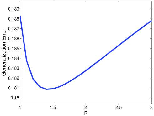
In real settings, it is likely that one uses various types of kernels and the complexities of RKHSs become inhomogeneous. As mentioned above, it has been often reported that $\ell_{1}$-MKL is outperformed by dense type MKL such as $\ell_{\frac{4}{3}}$-MKL in numerical experiments (Cortes et al., 2010). Our theoretical analysis in this section well support these experimental results.

6 Numerical Comparison between Homogeneous and Inhomogeneous Settings

Here we investigate numerically how the inhomogeneity of the complexities affects the performances using synthetic data. In particular, we numerically compare two situations: (a) all complexities of RKHSs are same (homogeneous situation) and (b) one RKHS is complex and other RKHSs are evenly simple (inhomogeneous situation).

The experimental settings are as follows. The input random variable is 20 dimensional vector $x=(x^{(1)},\dots,x^{(20)})$ where each element $x^{(m)}$ is independently identically distributed from the uniform distribution on $[0,1]$:

$$x^{(m)}\sim\mathrm{Unif}([0,1])~{}~{}~{}(m=1,\dots,20).$$

For each coordinate $m=1,\dots,20$, we put one Gaussian RKHS $\mathcal{H}_{m}$ with a Gaussian width $\sigma_{m}$: the number of kernels is 20 ($M=20$) and

$$k_{m}(x,x^{\prime})=\exp\left(-\frac{(x^{(m)}-{x^{\prime(m)}})^{2}}{2\sigma_{m}^{2}}\right)~{}~{}~{}(m=1,\dots,20),$$

for $x=(x^{(1)},\dots,x^{(20)})$ and $x^{\prime}=(x^{\prime(1)},\dots,x^{\prime(20)})$. To generate the ground truth $f^{*}$, we randomly generated 5 center points $\mu_{i,m}~{}(i=1,\dots,5)$ for each coordinate $m=1,\dots,20$ where $\mu_{i,m}$ is independently generated by the uniform distribution on $[0,1]$. Then we obtain the following form of the true function:

$$f^{*}(x) =\sum_{m=1}^{20}f^{*}_{m}(x),$$

$$\text{where}~{}~{}f^{*}_{m}(x) =\sum_{i=1}^{5}\alpha_{i,m}\exp\left(-\frac{(x^{(m)}-\mu_{i,m})^{2}}{2\sigma_{m}^{2}}\right)\in\mathcal{H}_{m},$$

for $x=(x_{1},\dots,x_{m})$. Each coefficient $\alpha_{i,m}$ is independently identically distributed from the standard normal distribution. The output $y$ is contaminated by a noise $\epsilon$ where the noise $\epsilon$ is distributed from the Gaussian distribution with mean 0 and standard deviation 0.1:

$$y=f^{*}_{m}(x)+\epsilon,$$

$$\epsilon\sim\mathcal{N}(0,0.1).$$

We generated 200 or 400 realizations $\{(x_{i},y_{i})\}_{i=1}^{n}$ ($n=200$ or $n=400$), and estimated $f^{*}$ using $\ell_{p}$-MKL with $p=1,1.1,1.2,\dots,3$ . The estimator is computed with various regularization parameters ${\lambda_{1}^{(n)}}$. The generalization error $\|\hat{f}-f^{*}\|_{L_{2}(\Pi)}^{2}$ was numerically calculated. We repeated the experiments for 100 times, averaged the generalization errors over 100 repetitions for each $p$ and each regularization parameter, and obtained the optimal average generalization error among all regularization parameters for each $p$. The true function was randomly generated for each repetition. We investigated the generalization errors in the following homogeneous and inhomogeneous settings:

1. (homogeneous) $\sigma_{m}=0.5$ for $m=1,\dots,20$.

2. (inhomogeneous) $\sigma_{1}=0.01$ and $\sigma_{m}=0.5$ for $m=2,\dots,20$.

The difference between the above homogeneous and inhomogeneous settings is the value of $\sigma_{1}$; whether $\sigma_{1}=0.5$ or $\sigma_{1}=0.01$. The inhomogeneous situation is analogous to that investigated in Sec.5 where we assumed one RKHS is complex and the other RKHSs are evenly simple (small $\sigma_{1}$ corresponds to a complex RKHS).

(a) Homogeneous Setting ($n=200$)

(b) Inhomogeneous Setting ($n=200$)

(c) Homogeneous Setting ($n=400$)

(d) Inhomogeneous Setting ($n=400$)

Figure 2: The expected generalization error $\mathrm{E}[\|\hat{f}-f^{*}\|_{L_{2}(\Pi)}^{2}]$ against the parameter $p$ for $\ell_{p}$-MKL. Each broken line corresponds to one regularization parameter. The bold solid line shows the best generalization error among all the regularization parameters.

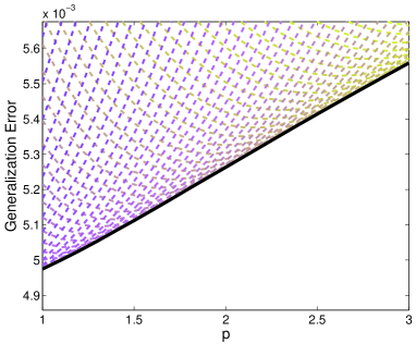
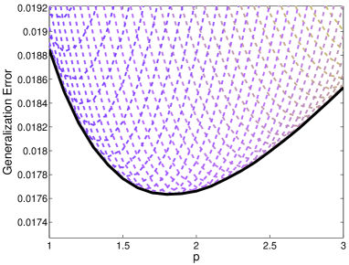
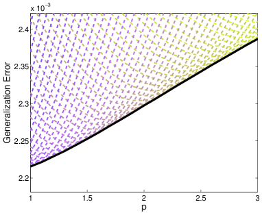
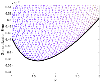
Figure 2 shows the average generalization errors in the homogeneous setting with (a) $n=200$ and (c) $n=400$, and the inhomogeneous setting with (b) $n=200$ and (d) $n=400$. Each broken line corresponds to one regularization parameter. The bold solid line shows the best (average) generalization error among all the regularization parameters. We can see that in the homogeneous setting $\ell_{1}$-regularization shows the best performance, on the other hand, in the inhomogeneous setting the best performance is achieved at $p>1$ for both $n=200$ and $400$. This experimental results beautifully matches the theoretical investigations.

7 Generalization of loss function

Here we discuss how a general loss function other than squared loss can be involved into our analysis. As in the standard local Rademacher complexity argument (Bartlett et al., 2005), we consider a class of loss functions that are Lipschitz continuous and strongly convex. Suppose that the loss function $\Psi:\mathbb{R}\times\mathbb{R}\to\mathbb{R}$ satisfies Lipschitz continuity: for all $R>0$, there exists a constant $T(R)$ such that

$$|\Psi(y,f_{1})-\Psi(y,f_{2})|\leq T(R)|f_{1}-f_{2}|~{}~{}~{}~{}(\forall f_{1},f_{2}\in\mathbb{R}~{}\text{such that $|f_{1}|,|f_{2}|\leq R$},~{}\forall y\in\mathbb{R}).$$ (20)

Moreover, suppose that, for all $y\in\mathbb{R}$, $\Psi(y,f)$ is a strongly convex with a modulus $\rho(R)>0$:

$$\frac{\Psi(y,f_{1})+\Psi(y,f_{2})}{2}\geq\Psi\left(y,\frac{f_{1}+f_{2}}{2}\right)+\frac{\rho(R)}{2}|f_{1}-f_{2}|^{2}$$

$$~{}~{}(\forall f_{1},f_{2}\in\mathbb{R}~{}\text{such that $|f_{1}|,|f_{2}|\leq R$}).$$ (21)

Some detailed discussions about these conditions and examples can be found in Bartlett et al. (2006). Under the loss functions satisfying these properties, we obtain simplified bound where some conditions can be omitted as follows:

• We can remove the condition $\frac{4\phi\sqrt{n}}{\kappa_{M}}\max\{\alpha_{1}^{2},\beta_{1}^{2},\frac{M\log(M)}{n}\}\eta(t^{\prime})\leq\frac{1}{12}$,

• The term $\exp(-t^{\prime})$ is not needed in the tail probability.

To obtain a fast convergence rate on a general loss functions $\Psi$, we move the regularization term in Eq. (1) into a constraint, and then consider the following optimization problem:

$$\hat{f}=\sum_{m=1}^{M}\hat{f}_{m}= \mathop{\arg\min}_{\begin{subarray}{c}~{}f_{m}\in\mathcal{H}_{m}~{}(m=1,\dots,M),\\ \|f\|_{\psi}\leq\hat{R}\end{subarray}}\frac{1}{n}\sum_{i=1}^{N}\Psi\left(y_{i},\sum_{m=1}^{M}f_{m}(x_{i})\right),$$ (22)

where $\hat{R}$ is a regularization parameter. The above optimization problem is essentially equivalent to the original formulation (1), but by considering the constraint type regularization instead of the penalty type regularization the theoretical analysis of statistical performance can be simplified.

We define $Pg$ as the expectation of a function $g:\mathbb{R}\times\mathbb{R}\to\mathbb{R}$:

$$Pg:=\mathrm{E}_{(X,Y)\sim P}[g(X,Y)].$$

For notational simplicity, we write $P\Psi(f)=P\Psi(Y,f)=\mathrm{E}_{(X,Y)\sim P}[\Psi(Y,f(X))]$ for a function $f$. We suppose there exists a minimizer for $P\Psi(f)$ as follows.

Assumption 7

(Minimizer Existence Assumption)
There exists unique $f^{*}=(f^{*}_{1},\dots,f^{*}_{M})\in\mathcal{H}^{\oplus M}$ such that

(A7) $$f^{*}=\sum_{m=1}^{M}f^{*}_{m}=\mathop{\arg\min}_{f_{m}\in\mathcal{H}_{m}~{}(m=1,\dots,M)}P\Psi\left(\sum_{m=1}^{M}f_{m}(X)\right).$$

Note that, due to the incoherence assumption (Assumption 4) and the strong convexity (21) of the loss function, if there exists a minimizer, then that is automatically unique.

To bound the convergence rate on a general loss function, it is convenient to utilize local Rademacher complexity on $\psi$-norm ball. Let $\mathcal{H}_{\psi}^{(r)}(R):=\{f\in\mathcal{H}^{\oplus M}\mid\|f\|_{L_{2}(\Pi)}\leq r,~{}\|f\|_{\psi}\leq R\}$. Then the local Rademacher complexity of $\mathcal{H}_{\psi}^{(r)}(R)$ is defined as

$$R_{n}(\mathcal{H}_{\psi}^{(r)}(R)):=\mathrm{E}_{\{\sigma_{i},x_{i}\}_{i=1}^{n}}\left[\sup_{f\in\mathcal{H}_{\psi}^{(r)}(R)}\frac{1}{n}\sum_{i=1}^{n}\sigma_{i}f(x_{i})\right],$$

where $\sigma_{i}\in\{\pm 1\}$ is the i.i.d. Rademacher random variable with $P(\sigma_{i}=1)=P(\sigma_{i}=-1)=\frac{1}{2}$. Evaluating the local Rademacher complexity is a key ingredient to show a fast convergence rate on a general loss function. We obtain the following estimation of the local Rademacher complexity (the proof will be given in Appendix F.4).

Lemma 6

Let $\{r_{m}\}_{m=1}^{M}$ be arbitrary positive reals. Under Assumptions 2-5, there exists a constant $\tilde{\phi}$ depending on $\{s_{m}\}_{m=1}^{M},c,C_{1}$ such that for all $n$ satisfying $\frac{\log(M)}{\sqrt{n}}\leq 1$ we have

$$R_{n}(\mathcal{H}_{\psi}^{(r)}(R))\leq\tilde{\phi}\left(\alpha_{1}\frac{r}{\sqrt{\kappa_{M}}}+\alpha_{2}R+\beta_{1}\frac{r}{\sqrt{\kappa_{M}}}+\beta_{2}R+\sqrt{\frac{M\log(M)}{n}}\frac{r}{\sqrt{\kappa_{M}}}\right).$$

Finally note that the supremum norm of $f$ with $\|f\|_{\psi}\leq\hat{R}$ can be bounded as

$$\|f\|_{\infty}\leq\sum_{m=1}^{M}\|f_{m}\|_{\infty}\leq\sum_{m=1}^{M}\|f_{m}\|_{\mathcal{H}_{m}}\leq\|\boldsymbol{1}\|_{\psi^{*}}\|f\|_{\psi}\leq\|\boldsymbol{1}\|_{\psi^{*}}\hat{R}.$$

Then, we obtain the excess risk bound as in the following theorem.

Theorem 7

Suppose Assumptions 2-5 and 7 are satisfied and the loss function $\Psi$ satisfies the conditions (20) and (21). Let $\{r_{m}\}_{m=1}^{M}$ be arbitrary positive reals that can depend on $n$ and let $\bar{T}=T(\|\boldsymbol{1}\|_{\psi^{*}}\hat{R})$ and $\bar{\rho}=\rho(\|\boldsymbol{1}\|_{\psi^{*}}\hat{R})$. Set $\hat{R}=\|f^{*}\|_{\psi}$. Then there exists a constant $\tilde{\phi}^{\prime}$ depending on $\{s_{m}\}_{m=1}^{M},c,C_{1}$ such that for all $n$ satisfying $\frac{\log(M)}{\sqrt{n}}\leq 1$, we have

$$P(\Psi(\hat{f})-\Psi(f^{*}_{\hat{R}}))$$

$$\leq \frac{\tilde{\phi}^{\prime}\bar{\rho}}{\kappa_{M}}\left(\alpha_{1}^{2}+\beta_{1}^{2}+\frac{M\log(M)}{n}\right)+\tilde{\phi}^{\prime}\frac{\bar{T}^{2}}{\bar{\rho}}\left[\left(\frac{\alpha_{2}}{\alpha_{1}}\right)^{2}+\left(\frac{\beta_{2}}{\beta_{1}}\right)^{2}\right]\|f^{*}\|_{\psi}^{2}$$

$$+\frac{\{22\bar{T}\|\boldsymbol{1}\|_{\psi^{*}}\hat{R}+27\bar{\rho}\}t}{n},$$ (23)

with probability $1-\exp(-t)$.

This can be shown by applying the bound of the local Rademacher complexity (Lemma 6) to Corollary 5.3 of Bartlett et al. (2005). Compared with the bound in Eq. (6), we notice that there is no $\exp(-t^{\prime})$ term in the tail probability bound, and thus we don’t need the condition $\frac{4\phi\sqrt{n}}{\kappa_{M}}\max\{\alpha_{1}^{2},\beta_{1}^{2},\frac{M\log(M)}{n}\}\eta(t^{\prime})\leq\frac{1}{12}$. Because of this, the range of $n$ where the error bound holds is relaxed compared with that in Theorem 1. These simplifications are due to the Lipschitz continuity of the loss function. In Theorem 1, we should have bounded the discrepancy between the empirical and population means of the squared loss: $\frac{1}{n}\sum_{i=1}^{n}(\hat{f}(x_{i})-f^{*}(x_{i}))^{2}-P(\hat{f}-f^{*})^{2}$. Since the squared loss is not Lipschitz continuous, we required an additional bound for that discrepancy using Assumption 5 for the supremum norm, and it was shown that that discrepancy is negligible at the cost of $\exp(-t^{\prime})$ in the tail probability. On the other hand, for Lipschitz continuous losses, we no longer need to bound such a quantity. Thus the tail probability loss $\exp(-t^{\prime})$ is not induced.

Since the bound (23) is basically same as Eq.(6), we obtain the same discussions as in the previous sections. For example, in the homogeneous setting, we obtain the following convergence bound.

Lemma 8

When $s_{m}=s~{}(\forall m)$ with some $0<s<1$, if we set $\hat{R}=\|f^{*}\|_{\psi}$, then for all $n$ satisfying $\frac{\log(M)}{\sqrt{n}}\leq 1$ and $n\geq(\|\boldsymbol{1}\|_{\psi^{*}}\|f^{*}\|_{\psi}/M)^{\frac{4s}{1-s}}$, and for all $t\geq 1$, we have

$$P(\Psi(\hat{f})-\Psi(f^{*}))\leq C\left\{M^{1-\frac{2s}{1+s}}n^{-\frac{1}{1+s}}(\|\boldsymbol{1}\|_{\psi^{*}}\|f^{*}\|_{\psi})^{\frac{2s}{1+s}}+\frac{M\log(M)}{n}+\frac{t}{n}\right\},$$

with probability $1-\exp(-t)$ where $C$ is a constant depending on $\tilde{\phi}^{\prime}$, $\kappa_{M}$, $\rho(\|\boldsymbol{1}\|_{\psi^{*}}\hat{R})$, and $T(\|\boldsymbol{1}\|_{\psi^{*}}\hat{R})$.

8 Conclusion and Future Work

We have shown a unifying framework to derive the learning rate of MKL with arbitrary mixed-norm-type regularization. To analyze the general result, we considered two situations: homogeneous settings and inhomogeneous settings. We have seen that the convergence rate of $\ell_{p}$-MKL obtained in homogeneous settings is tighter and requires less restrictive condition than existing results. We have also shown convergence rates of some examples (elasticnet-MKL and VSKL), and proved the derived learning rate is minimax optimal when $\psi$-norm is isotropic. An interesting consequence was that $\ell_{1}$-regularization is optimal among all isotropic $\psi$-norm regularization in homogeneous settings. In the analysis of inhomogeneous settings, we have shown that the dense type regularization can outperform the sparse $\ell_{1}$-regularization using analytically obtained bounds and numerically computed bounds. We observed that our bound well explains the experimental results favorable for dense type MKL. Finally we numerically investigated the generalization errors of $\ell_{p}$-MKL in a homogeneous setting and an inhomogeneous setting. The numerical experiments supported the theoretical findings that $\ell_{1}$-regularization is optimal in homogeneous settings but, on the other hand, dense type regularizations are preferred in inhomogeneous settings. This is the first result that suggests that the inhomogeneity of the complexities of RKHSs well justifies the favorable performances for dense type MKL.

An interesting future work is about the $\frac{M\log(M)}{n}$ term appeared in the bound Eq. (8). Because of this term, our bound is $O(M\log(M))$ with respect to $M$ while in the existing work that is $O(\sqrt{\log(M)}\vee M^{1-\frac{1}{p}})$ for $\ell_{p}$-MKL. Therefore our bound is not tight in the global bound regime ($n\leq M^{\frac{2}{p}}R_{p}^{-2}\log(M)^{\frac{1+s}{s}}$ for $\ell_{p}$-MKL). It is an interesting issue to clarify whether the term $\frac{M\log(M)}{n}$ can be replaced by other tighter bounds or not. To do so, it might be helpful to combine our technique developed in this paper and that developed by Kloft and Blanchard (2011) where the local Rademacher complexity for $\ell_{p}$-MKL is derived.

A Relation between Entropy Number and Spectral Condition

Associated with the $\epsilon$-covering number, the $i$-th entropy number $e_{i}(\mathcal{H}_{m}\to L_{2}(\Pi))$ is defined as the infimum over all $\varepsilon>0$ for which $N(\varepsilon,\mathcal{B}_{\mathcal{H}_{m}},L_{2}(\Pi))\leq 2^{i-1}$. If the spectral assumption (A3) and the boundedness assumption (A2) hold, the relation (2) implies that the $i$-th entropy number is bounded as

$$e_{i}(\mathcal{H}_{m}\to L_{2}(\Pi))\leq Ci^{-\frac{1}{2s}},$$ (24)

where $C$ is a constant. To bound empirical process a bound of the entropy number with respect to the empirical distribution is needed. The following proposition gives an upper bound of that (see Corollary 7.31 of Steinwart (2008), for example).

Proposition 9

If there exists constants $0<s<1$ and $C\geq 1$ such that $e_{i}(\mathcal{H}_{m}\to L_{2}(\Pi))\leq Ci^{-\frac{1}{2s}}$, then there exists a constant $c_{s}>0$ only depending on $s$ such that

$$\mathrm{E}_{D_{n}\sim\Pi^{n}}[e_{i}(\mathcal{H}_{m}\to L_{2}(D_{n}))]\leq c_{s}C(\min(i,n))^{\frac{1}{2s}}i^{-\frac{1}{s}},$$

in particular $\mathrm{E}_{D_{n}\sim\Pi^{n}}[e_{i}(\mathcal{H}_{m}\to L_{2}(D_{n}))]\leq c_{s}Ci^{-\frac{1}{2s}}.$

B Basic Propositions

The following two propositions are keys to prove Theorem 1. Let $\{\sigma_{i}\}_{i=1}^{n}$ be i.i.d. Rademacher random variables, i.e., $\sigma_{i}\in\{\pm 1\}$ and $P(\sigma_{i}=1)=P(\sigma_{i}=-1)=\frac{1}{2}$.

Proposition 10

(Steinwart, 2008, Theorem 7.16) Let $\mathcal{B}_{\sigma,a,b}\subset\mathcal{H}_{m}$ be a set such that $\mathcal{B}_{\sigma,a,b}=\{f_{m}\in\mathcal{H}_{m}\mid\|f_{m}\|_{L_{2}(\Pi)}\leq\sigma,\|f_{m}\|_{\mathcal{H}_{m}}\leq a,\|f_{m}\|_{\infty}\leq b\}$. Assume that there exist constants $0<s<1$ and $0<\tilde{c}_{s}$ such that

$$\mathrm{E}_{D_{n}}[e_{i}(\mathcal{H}_{m}\to L_{2}(D_{n}))]\leq\tilde{c}_{s}i^{-\frac{1}{2s}}.$$

Then there exists a constant $C_{s}^{\prime}$ depending only $s$ such that

$$\mathrm{E}\left[\sup_{f_{m}\in\mathcal{B}_{\sigma,a,b}}\left|\frac{1}{n}\sum_{i=1}^{n}\sigma_{i}f_{m}(x_{i})\right|\right]\leq C_{s}^{\prime}\left(\frac{\sigma^{1-s}(\tilde{c}_{s}a)^{s}}{\sqrt{n}}\vee(\tilde{c}_{s}a)^{\frac{2s}{1+s}}b^{\frac{1-s}{1+s}}n^{-\frac{1}{1+s}}\right).$$ (25)

Proposition 11

(Talagrand’s Concentration Inequality Talagrand (1996); Bousquet (2002)) Let $\mathcal{G}$ be a function class on $\mathcal{X}$ that is separable with respect to $\infty$-norm, and $\{x_{i}\}_{i=1}^{n}$ be i.i.d. random variables with values in $\mathcal{X}$. Furthermore, let $B\geq 0$ and $U\geq 0$ be $B:=\sup_{g\in\mathcal{G}}\mathrm{E}[(g-\mathrm{E}[g])^{2}]$ and $U:=\sup_{g\in\mathcal{G}}\|g\|_{\infty}$, then there exists a universal constant $K$ such that, for $Z:=\sup_{g\in\mathcal{G}}\left|\frac{1}{n}\sum_{i=1}^{n}g(x_{i})-\mathrm{E}[g]\right|$, we have

$$P\left(Z\geq K\left[\mathrm{E}[Z]+\sqrt{\frac{Bt}{n}}+\frac{Ut}{n}\right]\right)\leq e^{-t}.$$

C Proof of Theorem 1

Let $r_{m}>0~{}(m=1,\dots,M)$ be arbitrary positive reals. Given $\{r_{m}\}_{m=1}^{M}$, we determine $U_{n,s_{m}}^{(m)}(f_{m})$ as follows:

$$U_{n,s_{m}}^{(m)}(f_{m}):= 3\left(\frac{r_{m}^{-s_{m}}}{\sqrt{n}}\vee\frac{r_{m}^{-\frac{s_{m}(3-s_{m})}{1+s_{m}}}}{n^{\frac{1}{1+s_{m}}}}\right)\left(\|f_{m}\|_{L_{2}(\Pi)}+s_{m}r_{m}\|f_{m}\|_{\mathcal{H}_{m}}\right)+\sqrt{\frac{\log(M)}{n}}\|f_{m}\|_{L_{2}(\Pi)}.$$

It is easy to see $U_{n,s_{m}}^{(m)}(f_{m})$ is an upper bound of the quantity $\frac{\|f_{m}\|_{L_{2}(\Pi)}^{1-s_{m}}\|f_{m}\|_{\mathcal{H}_{m}}^{s_{m}}}{\sqrt{n}}\vee\frac{\|f_{m}\|_{L_{2}(\Pi)}^{\frac{(1-s_{m})^{2}}{1+s_{m}}}\|f_{m}\|_{\mathcal{H}_{m}}^{\frac{s_{m}(3-s_{m})}{1+s_{m}}}}{n^{\frac{1}{1+s_{m}}}}$ (this corresponds to the RHS of Eq. (25)) because

$$\frac{\|f_{m}\|_{L_{2}(\Pi)}^{1-s_{m}}\|f_{m}\|_{\mathcal{H}_{m}}^{s_{m}}}{\sqrt{n}} =\frac{r_{m}^{1-s_{m}}}{\sqrt{n}}\left(\frac{\|f_{m}\|_{L_{2}(\Pi)}}{r_{m}}\right)^{1-s_{m}}\|f_{m}\|_{\mathcal{H}_{m}}^{s_{m}}$$

$$\mathop{\leq}^{\rm(Young)}\frac{r_{m}^{1-s_{m}}}{\sqrt{n}}\left((1-s_{m})\frac{\|f_{m}\|_{L_{2}(\Pi)}}{r_{m}}+s_{m}\|f_{m}\|_{\mathcal{H}_{m}}\right)$$

$$\leq\frac{r_{m}^{-s_{m}}}{\sqrt{n}}\left(\|f_{m}\|_{L_{2}(\Pi)}+s_{m}r_{m}\|f_{m}\|_{\mathcal{H}_{m}}\right),$$ (26)

where we used Young’s inequality $a^{1-s_{m}}b^{s_{m}}\leq(1-s_{m})a+s_{m}b$ in the second line, and similarly we obtain

$$\frac{\|f_{m}\|_{L_{2}(\Pi)}^{\frac{(1-s_{m})^{2}}{1+s_{m}}}\|f_{m}\|_{\mathcal{H}_{m}}^{\frac{s_{m}(3-s_{m})}{1+s_{m}}}}{n^{\frac{1}{1+s_{m}}}} \leq\frac{r_{m}^{-\frac{s_{m}(3-s_{m})}{1+s_{m}}}}{n^{\frac{1}{1+s_{m}}}}\left(\|f_{m}\|_{L_{2}(\Pi)}+\frac{s_{m}(3-s_{m})}{1+s_{m}}r_{m}\|f_{m}\|_{\mathcal{H}_{m}}\right)$$

$$\leq 3\frac{r_{m}^{-\frac{s_{m}(3-s_{m})}{1+s_{m}}}}{n^{\frac{1}{1+s_{m}}}}\left(\|f_{m}\|_{L_{2}(\Pi)}+s_{m}r_{m}\|f_{m}\|_{\mathcal{H}_{m}}\right),$$

where we used $\frac{s_{m}(3-s_{m})}{1+s_{m}}\leq 3s_{m}$ in the last inequality.

Now we define

$$\phi:=\max\left(KL\left[2\tilde{C}_{*}+1+C_{1}\right],K\left[2C_{1}\tilde{C}_{*}+C_{1}+C_{1}^{2}\right]\right),$$

where $\tilde{C}^{*}$ is a constant defined later in Lemma 16, $C_{1}$ is the one introduced in Assumption 5, $K$ is the universal constant appeared in Talagrand’s concentration inequality (Proposition 11) and $L$ is the one introduced in Assumption 1 to bound the magnitude of noise. Remind the definition of $\eta(t)$:

$$\eta(t):=\eta_{n}(t)=\max(1,\sqrt{t},t/\sqrt{n}).$$

We define events $\mathscr{E}_{1}(t)$ and $\mathscr{E}_{2}(t^{\prime})$ as

$$\mathscr{E}_{1}(t)=\left\{\left|\frac{1}{n}\sum_{i=1}^{n}\epsilon_{i}f_{m}(x_{i})\right|\leq\phi U_{n,s_{m}}^{(m)}(f_{m})\eta(t),~{}\forall f_{m}\in\mathcal{H}_{m}~{}(m=1,\dots,M)\right\},$$ (27)

$$\mathscr{E}_{2}(t^{\prime})=\Bigg{\{}\left|\textstyle\left\|\sum_{m=1}^{M}f_{m}\right\|_{n}^{2}-\left\|\sum_{m=1}^{M}f_{m}\right\|_{L_{2}(\Pi)}^{2}\right|\leq\phi\sqrt{n}\left(\sum_{m=1}^{M}U_{n,s_{m}}^{(m)}(f_{m})\right)^{2}\eta(t^{\prime}),$$

$$~{}~{}~{}~{}~{}~{}~{}~{}~{}~{}~{}~{}~{}~{}~{}~{}~{}~{}~{}~{}~{}~{}~{}~{}~{}~{}~{}~{}~{}~{}~{}~{}~{}~{}~{}\forall f_{m}\in\mathcal{H}_{m}~{}(m=1,\dots,M)\Bigg{\}}.$$ (28)

Using Lemmas 17 and 18 that will be shown in Appendix D, we see that the events $\mathscr{E}_{1}(t)$ and $\mathscr{E}_{2}(t^{\prime})$ occur with probability no less than $1-\exp(-t)$ and $1-\exp(-t^{\prime})$ respectively as in the following Lemma.

Lemma 12

Under the Basic Assumption (Assumption 1), the Spectral Assumption (Assumption 3) and the Embedded Assumption (Assumption 5), the probabilities of $\mathscr{E}_{1}(t)$ and $\mathscr{E}_{2}$ are bounded as

$$P(\mathscr{E}_{1}(t))\geq 1-\exp(-t),~{}~{}~{}P(\mathscr{E}_{2}(t^{\prime}))\geq 1-\exp(-t^{\prime}).$$

Proof  Lemma 18 immediately gives $P(\mathscr{E}_{1}(t))\geq 1-\exp(-t)$ by noticing $\bar{\phi}$ in the statement of Lemma 18 satisfies $\bar{\phi}\leq\phi$. Moreover, since $\bar{\phi}^{\prime}$ in the statement of Lemma 17 satisfies $\bar{\phi}^{\prime}\leq\phi$, we have $P(\mathscr{E}_{2}(t^{\prime}))\geq 1-\exp(-t^{\prime})$ by Lemma 17.  

Remind the definition (4) of $\alpha_{1},\alpha_{2},\beta_{1},\beta_{2}$:

$$\alpha_{1}=3\left(\sum_{m=1}^{M}\frac{r_{m}^{-2s_{m}}}{n}\right)^{\frac{1}{2}},~{}~{}\alpha_{2}=3\left\|\left(\frac{s_{m}r_{m}^{1-s_{m}}}{\sqrt{n}}\right)_{m=1}^{M}\right\|_{\psi^{*}},$$

$$\beta_{1}=3\left(\sum_{m=1}^{M}\frac{r_{m}^{-\frac{2s_{m}(3-s_{m})}{1+s_{m}}}}{n^{\frac{2}{1+s_{m}}}}\right)^{\frac{1}{2}},~{}~{}\beta_{2}=3\left\|\left(\frac{s_{m}r_{m}^{\frac{(1-s_{m})^{2}}{1+s_{m}}}}{n^{\frac{1}{1+s_{m}}}}\right)_{m=1}^{M}\right\|_{\psi^{*}},$$ (29)

for given reals $\{r_{m}\}_{m=1}^{M}$. The following theorem immediately gives Theorem 1.

Theorem 13

Suppose Assumptions 1-4 are satisfied. Let $\{r_{m}\}_{m=1}^{M}$ be arbitrary positive reals that can depend on $n$, and assume ${\lambda_{1}^{(n)}}\geq\left(\frac{\alpha_{2}}{\alpha_{1}}\right)^{2}+\left(\frac{\beta_{2}}{\beta_{1}}\right)^{2}$. Then for all $n$ and $t^{\prime}$ that satisfy $\frac{\log(M)}{\sqrt{n}}\leq 1$ and $\frac{4\phi\sqrt{n}}{\kappa_{M}}\max\{\alpha_{1}^{2},\beta_{1}^{2},\frac{M\log(M)}{n}\}\eta(t^{\prime})\leq\frac{1}{12}$ and for all $t\geq 1$, we have

$$\|\hat{f}-f^{*}\|_{L_{2}(\Pi)}^{2}\leq\frac{24\eta(t)^{2}\phi^{2}}{\kappa_{M}}\left(\alpha_{1}^{2}+\beta_{1}^{2}+\frac{M\log(M)}{n}\right)+4{\lambda_{1}^{(n)}}\|f^{*}\|_{\psi}^{2}.$$

with probability $1-\exp(-t)-\exp(-t^{\prime})$.

Proof  [Proof of Theorem 13] By the assumption of the theorem, we can assume Lemma 12 holds, that is, the event $\mathscr{E}_{1}(t)\cap\mathscr{E}_{2}(t^{\prime})$ occurs with probability $1-\exp(-t)-\exp(-t^{\prime})$. Below we discuss on the event $\mathscr{E}_{1}(t)\cap\mathscr{E}_{2}(t^{\prime})$.

Since $y_{i}=f^{*}(x_{i})+\epsilon_{i}$, we have

$$\|\hat{f}-f^{*}\|_{L_{2}(\Pi)}^{2}+{\lambda_{1}^{(n)}}\|\hat{f}\|_{\psi}^{2}$$

$$\leq (\|\hat{f}-f^{*}\|_{L_{2}(\Pi)}^{2}-\|\hat{f}-f^{*}\|_{n}^{2})+\frac{2}{n}\sum_{i=1}^{n}\sum_{m=1}^{M}\epsilon_{i}(\hat{f}_{m}(x_{i})-f^{*}_{m}(x_{i}))+{\lambda_{1}^{(n)}}\left\|f^{*}\right\|_{\psi}^{2}.$$

Here on the event $\mathscr{E}_{2}(t^{\prime})$, the above inequality gives

$$\|\hat{f}-f^{*}\|_{L_{2}(\Pi)}^{2}+{\lambda_{1}^{(n)}}\|\hat{f}\|_{\psi}^{2}$$

$$\leq \phi\sqrt{n}\left(\sum_{m=1}^{M}U_{n,s_{m}}^{(m)}(\hat{f}_{m}-f^{*}_{m})\right)^{2}\eta(t^{\prime})\!+\!\frac{2}{n}\sum_{i=1}^{n}\sum_{m=1}^{M}\epsilon_{i}(\hat{f}_{m}(x_{i})-f^{*}_{m}(x_{i}))+{\lambda_{1}^{(n)}}\|f^{*}\|_{\psi}^{2}.$$ (30)

Before we prove the statements, we show an upper bound of $\sum_{m=1}^{M}U_{n,s_{m}}^{(m)}(f_{m})$ required in the proof. By definition, we have

$$U_{n,s_{m}}^{(m)}(f_{m})$$

$$= 3\left(\frac{r_{m}^{-s_{m}}}{\sqrt{n}}\vee\frac{r_{m}^{-\frac{s_{m}(3-s_{m})}{1+s_{m}}}}{n^{\frac{1}{1+s_{m}}}}\right)\left(\|f_{m}\|_{L_{2}(\Pi)}+s_{m}r_{m}\|f_{m}\|_{\mathcal{H}_{m}}\right)+\sqrt{\frac{\log(M)}{n}}\|f_{m}\|_{L_{2}(\Pi)}$$

$$\leq 3\frac{r_{m}^{-s_{m}}}{\sqrt{n}}\left(\|f_{m}\|_{L_{2}(\Pi)}+s_{m}r_{m}\|f_{m}\|_{\mathcal{H}_{m}}\right)+3\frac{r_{m}^{-\frac{s_{m}(3-s_{m})}{1+s_{m}}}}{n^{\frac{1}{1+s_{m}}}}\left(\|f_{m}\|_{L_{2}(\Pi)}+s_{m}r_{m}\|f_{m}\|_{\mathcal{H}_{m}}\right)$$ (31)

$$+\sqrt{\frac{\log(M)}{n}}\|f_{m}\|_{L_{2}(\Pi)}.$$ (32)

Now the sum of the first term is bounded as

$$\sum_{m=1}^{M}3\frac{r_{m}^{-s_{m}}}{\sqrt{n}}\left(\|f_{m}\|_{L_{2}(\Pi)}+s_{m}r_{m}\|f_{m}\|_{\mathcal{H}_{m}}\right)$$

$$= 3\sum_{m=1}^{M}\frac{r_{m}^{-s_{m}}}{\sqrt{n}}\|f_{m}\|_{L_{2}(\Pi)}+3\sum_{m=1}^{M}\frac{s_{m}r_{m}^{1-s_{m}}}{\sqrt{n}}\|f_{m}\|_{\mathcal{H}_{m}}$$

$$\leq 3\left(\sum_{m=1}^{M}\frac{r_{m}^{-2s_{m}}}{n}\right)^{\frac{1}{2}}\left(\sum_{m=1}^{M}\|f_{m}\|_{L_{2}(\Pi)}^{2}\right)^{\frac{1}{2}}+3\left\|\left(\frac{s_{m}r_{m}^{1-s_{m}}}{\sqrt{n}}\right)_{m=1}^{M}\right\|_{\psi^{*}}\|f\|_{\psi},$$

where we used Cauchy-Schwarz inequality and the duality of the norm in the last inequality. The sum of the second term of the RHS of Eq. (32) is bounded as

$$\sum_{m=1}^{M}3\frac{r_{m}^{-\frac{s_{m}(3-s_{m})}{1+s_{m}}}}{n^{\frac{1}{1+s_{m}}}}\left(\|f_{m}\|_{L_{2}(\Pi)}+s_{m}r_{m}\|f_{m}\|_{\mathcal{H}_{m}}\right)$$

$$= 3\sum_{m=1}^{M}\frac{r_{m}^{-\frac{s_{m}(3-s_{m})}{1+s_{m}}}}{n^{\frac{1}{1+s_{m}}}}\|f_{m}\|_{L_{2}(\Pi)}+3\sum_{m=1}^{M}\frac{s_{m}r_{m}^{\frac{(1-s_{m})^{2}}{1+s_{m}}}}{n^{\frac{1}{1+s_{m}}}}\|f_{m}\|_{\mathcal{H}_{m}}$$

$$\leq 3\left(\sum_{m=1}^{M}\frac{r_{m}^{-\frac{2s_{m}(3-s_{m})}{1+s_{m}}}}{n^{\frac{2}{1+s_{m}}}}\right)^{\frac{1}{2}}\left(\sum_{m=1}^{M}\|f_{m}\|_{L_{2}(\Pi)}^{2}\right)^{\frac{1}{2}}+3\left\|\left(\frac{s_{m}r_{m}^{\frac{(1-s_{m})^{2}}{1+s_{m}}}}{n^{\frac{1}{1+s_{m}}}}\right)_{m=1}^{M}\right\|_{\psi^{*}}\|f\|_{\psi},$$

where we used Cauchy-Schwarz inequality and the duality of the norm in the last inequality. Finally we have the following bound of the third term of the RHS of Eq. (32):

$$\sum_{m=1}^{M}\sqrt{\frac{\log(M)}{n}}\|f_{m}\|_{L_{2}(\Pi)}\leq\sqrt{\frac{M\log(M)}{n}}\left(\sum_{m=1}^{M}\|f_{m}\|_{L_{2}(\Pi)}^{2}\right)^{\frac{1}{2}}.$$

Combine these inequalities and the relation $\sum_{m=1}^{M}\|f_{m}\|_{L_{2}(\Pi)}^{2}\leq\frac{1}{\kappa_{M}}\|f\|_{L_{2}(\Pi)}^{2}$ (Assumption 4) to obtain

$$\sum_{m=1}^{M}U_{n,s_{m}}^{(m)}(f_{m})$$

$$\leq 3\left(\sum_{m=1}^{M}\frac{r_{m}^{-2s_{m}}}{n}\right)^{\frac{1}{2}}\frac{\|f\|_{L_{2}(\Pi)}}{\sqrt{\kappa_{M}}}+3\left\|\left(\frac{s_{m}r_{m}^{1-s_{m}}}{\sqrt{n}}\right)_{m=1}^{M}\right\|_{\psi^{*}}\|f\|_{\psi}$$

$$+3\left(\sum_{m=1}^{M}\frac{r_{m}^{-\frac{2s_{m}(3-s_{m})}{1+s_{m}}}}{n^{\frac{2}{1+s_{m}}}}\right)^{\frac{1}{2}}\frac{\|f\|_{L_{2}(\Pi)}}{\sqrt{\kappa_{M}}}+3\left\|\left(\frac{s_{m}r_{m}^{\frac{(1-s_{m})^{2}}{1+s_{m}}}}{n^{\frac{1}{1+s_{m}}}}\right)_{m=1}^{M}\right\|_{\psi^{*}}\|f\|_{\psi}$$

$$+\sqrt{\frac{M\log(M)}{n}}\frac{\|f\|_{L_{2}(\Pi)}}{\sqrt{\kappa_{M}}}.$$ (33)

Then by the definition (4) of $\alpha_{1},\alpha_{2},\beta_{1},\beta_{2}$, we have

$$\sum_{m=1}^{M}U_{n,s_{m}}^{(m)}(f_{m})$$

$$\leq \alpha_{1}\frac{\|f\|_{L_{2}(\Pi)}}{\sqrt{\kappa_{M}}}+\alpha_{2}\|f\|_{\psi}+\beta_{1}\frac{\|f\|_{L_{2}(\Pi)}}{\sqrt{\kappa_{M}}}+\beta_{2}\|f\|_{\psi}+\sqrt{\frac{M\log(M)}{n}}\frac{\|f\|_{L_{2}(\Pi)}}{\sqrt{\kappa_{M}}}.$$ (34)

Step 1.

By Eq. (34), the first term on the RHS of Eq. (30) can be upper bounded as

$$\phi\sqrt{n}\left(\sum_{m=1}^{M}U_{n,s_{m}}^{(m)}(\hat{f}_{m}-f^{*}_{m})\right)^{2}\eta(t^{\prime})$$

$$\leq 4\phi\sqrt{n}\Big{(}\alpha_{1}^{2}\frac{\|\hat{f}-f^{*}\|_{L_{2}(\Pi)}^{2}}{\kappa_{M}}+\alpha_{2}^{2}\|\hat{f}-f^{*}\|_{\psi}^{2}+\beta_{1}^{2}\frac{\|\hat{f}-f^{*}\|_{L_{2}(\Pi)}^{2}}{\kappa_{M}}+$$

$$~{}~{}~{}~{}~{}~{}~{}~{}~{}~{}~{}~{}~{}~{}~{}\beta_{2}^{2}\|\hat{f}-f^{*}\|_{\psi}^{2}+\frac{M\log(M)}{n}\frac{\|\hat{f}-f^{*}\|_{L_{2}(\Pi)}^{2}}{\kappa_{M}}\Big{)}\eta(t^{\prime})$$

$$\leq \frac{4\phi\sqrt{n}}{\kappa_{M}}\alpha_{1}^{2}\eta(t^{\prime})\left(\|\hat{f}-f^{*}\|_{L_{2}(\Pi)}^{2}+\left(\frac{\alpha_{2}}{\alpha_{1}}\right)^{2}\|\hat{f}-f^{*}\|_{\psi}^{2}\right)$$

$$+\frac{4\phi\sqrt{n}}{\kappa_{M}}\beta_{1}^{2}\eta(t^{\prime})\left(\|\hat{f}-f^{*}\|_{L_{2}(\Pi)}^{2}+\left(\frac{\beta_{2}}{\beta_{1}}\right)^{2}\|\hat{f}-f^{*}\|_{\psi}^{2}\right)$$

$$+\frac{4\phi\sqrt{n}}{\kappa_{M}}\frac{M\log(M)}{n}\eta(t^{\prime})\|\hat{f}-f^{*}\|_{L_{2}(\Pi)}^{2}.$$

By assumption, we have $\frac{4\phi\sqrt{n}}{\kappa_{M}}\max\{\alpha_{1}^{2},\beta_{1}^{2},\frac{M\log(M)}{n}\}\eta(t^{\prime})\leq\frac{1}{12}$. Hence the RHS of the above inequality is bounded by

$$\phi\sqrt{n}\left(\sum_{m=1}^{M}U_{n,s_{m}}^{(m)}(\hat{f}_{m}-f^{*}_{m})\right)^{2}\eta(t^{\prime})$$

$$\leq \frac{1}{4}\left\{\|\hat{f}-f^{*}\|_{L_{2}(\Pi)}^{2}+\left[\left(\frac{\alpha_{2}}{\alpha_{1}}\right)^{2}+\left(\frac{\beta_{2}}{\beta_{1}}\right)^{2}\right]\|\hat{f}-f^{*}\|_{\psi}^{2}\right\}.$$ (35)

Step 2. On the event $\mathscr{E}_{1}(t)$, we have

$$\phantom{\leq}\frac{2}{n}\sum_{i=1}^{n}\sum_{m=1}^{M}\epsilon_{i}(\hat{f}_{m}(x_{i})-f^{*}_{m}(x_{i}))\leq 2\sum_{m=1}^{M}\eta(t)\phi U_{n,s_{m}}^{(m)}(\hat{f}_{m}-f^{*}_{m})$$

$$\leq 2\eta(t)\phi\Bigg{[}\alpha_{1}\frac{\|\hat{f}-f^{*}\|_{L_{2}(\Pi)}}{\sqrt{\kappa_{M}}}+\alpha_{2}\|\hat{f}-f^{*}\|_{\psi}+\beta_{1}\frac{\|\hat{f}-f^{*}\|_{L_{2}(\Pi)}}{\sqrt{\kappa_{M}}}+\beta_{2}\|\hat{f}-f^{*}\|_{\psi}$$

$$~{}~{}~{}~{}+\sqrt{\frac{M\log(M)}{n}}\frac{\|\hat{f}-f^{*}\|_{L_{2}(\Pi)}}{\sqrt{\kappa_{M}}}\Bigg{]}~{}~{}~{}~{}~{}~{}~{}~{}~{}~{}~{}~{}~{}~{}~{}~{}~{}~{}~{}~{}~{}~{}~{}~{}~{}~{}~{}~{}~{}~{}~{}~{}~{}~{}~{}(\because\text{Eq.\eqref{eq:UnsmBoundAlphaBeta}})$$

$$\leq 2\frac{\eta(t)\phi\alpha_{1}}{\sqrt{\kappa_{M}}}\left(\|\hat{f}-f^{*}\|_{L_{2}(\Pi)}+\frac{\alpha_{2}}{\alpha_{1}}\|\hat{f}-f^{*}\|_{\psi}\right)+2\frac{\eta(t)\phi\beta_{1}}{\sqrt{\kappa_{M}}}\left(\|\hat{f}-f^{*}\|_{L_{2}(\Pi)}+\frac{\beta_{2}}{\beta_{1}}\|\hat{f}-f^{*}\|_{\psi}\right)$$

$$~{}~{}~{}~{}+2\frac{\eta(t)\phi}{\sqrt{\kappa_{M}}}\sqrt{\frac{M\log(M)}{n}}\|\hat{f}-f^{*}\|_{L_{2}(\Pi)}$$

$$\leq\frac{12\eta(t)^{2}\phi^{2}\alpha_{1}^{2}}{\kappa_{M}}+\frac{1}{24}\left(\|\hat{f}-f^{*}\|_{L_{2}(\Pi)}+\frac{\alpha_{2}}{\alpha_{1}}\|\hat{f}-f^{*}\|_{\psi}\right)^{2}$$

$$~{}~{}~{}~{}~{}~{}+\frac{12\eta(t)^{2}\phi^{2}\beta_{1}^{2}}{\kappa_{M}}+\frac{1}{24}\left(\|\hat{f}-f^{*}\|_{L_{2}(\Pi)}+\frac{\beta_{2}}{\beta_{1}}\|\hat{f}-f^{*}\|_{\psi}\right)^{2}$$

$$~{}~{}~{}~{}~{}~{}+\frac{6\eta(t)^{2}\phi^{2}}{\kappa_{M}}\frac{M\log(M)}{n}+\frac{1}{12}\|\hat{f}-f^{*}\|_{L_{2}(\Pi)}^{2}$$

$$\leq\frac{12\eta(t)^{2}\phi^{2}\alpha_{1}^{2}}{\kappa_{M}}+\frac{1}{12}\left[\|\hat{f}-f^{*}\|_{L_{2}(\Pi)}^{2}+\left(\frac{\alpha_{2}}{\alpha_{1}}\right)^{2}\|\hat{f}-f^{*}\|_{\psi}^{2}\right]$$

$$~{}~{}~{}~{}~{}~{}+\frac{12\eta(t)^{2}\phi^{2}\beta_{1}^{2}}{\kappa_{M}}+\frac{1}{12}\left[\|\hat{f}-f^{*}\|_{L_{2}(\Pi)}^{2}+\left(\frac{\beta_{2}}{\beta_{1}}\right)^{2}\|\hat{f}-f^{*}\|_{\psi}^{2}\right]$$

$$~{}~{}~{}~{}~{}~{}+\frac{6\eta(t)^{2}\phi^{2}}{\kappa_{M}}\frac{M\log(M)}{n}+\frac{1}{12}\|\hat{f}-f^{*}\|_{L_{2}(\Pi)}^{2}$$

$$\leq\frac{12\eta(t)^{2}\phi^{2}}{\kappa_{M}}\left(\alpha_{1}^{2}+\beta_{1}^{2}+\frac{M\log(M)}{n}\right)+\frac{1}{4}\left\{\|\hat{f}-f^{*}\|_{L_{2}(\Pi)}^{2}+\left[\left(\frac{\alpha_{2}}{\alpha_{1}}\right)^{2}+\left(\frac{\beta_{2}}{\beta_{1}}\right)^{2}\right]\|\hat{f}-f^{*}\|_{\psi}^{2}\right\}.$$ (36)

Step 3.

Substituting the inequalities (35) and (36) to Eq. (30), we obtain

$$\|\hat{f}-f^{*}\|_{L_{2}(\Pi)}^{2}+{\lambda_{1}^{(n)}}\|\hat{f}\|_{\psi}^{2}$$

$$\leq \frac{12\eta(t)^{2}\phi^{2}}{\kappa_{M}}\left(\alpha_{1}^{2}+\beta_{1}^{2}+\frac{M\log(M)}{n}\right)+\frac{1}{2}\left\{\|\hat{f}-f^{*}\|_{L_{2}(\Pi)}^{2}+\left[\left(\frac{\alpha_{2}}{\alpha_{1}}\right)^{2}+\left(\frac{\beta_{2}}{\beta_{1}}\right)^{2}\right]\|\hat{f}-f^{*}\|_{\psi}^{2}\right\}$$

$$+{\lambda_{1}^{(n)}}\|f^{*}\|_{\psi}^{2}.$$ (37)

Now, by the triangular inequality, the term $\|\hat{f}-f^{*}\|_{\psi}^{2}$ can be bounded as

$$\|\hat{f}-f^{*}\|_{\psi}^{2}\leq\left(\|\hat{f}\|_{\psi}+\|f^{*}\|_{\psi}\right)^{2}\leq 2\left(\|\hat{f}\|_{\psi}^{2}+\|f^{*}\|_{\psi}^{2}\right).$$

Thus, when ${\lambda_{1}^{(n)}}\geq\left(\frac{\alpha_{2}}{\alpha_{1}}\right)^{2}+\left(\frac{\beta_{2}}{\beta_{1}}\right)^{2}$, Eq. (37) yields

$$\frac{1}{2}\|\hat{f}-f^{*}\|_{L_{2}(\Pi)}^{2}\leq\frac{12\eta(t)^{2}\phi^{2}}{\kappa_{M}}\left(\alpha_{1}^{2}+\beta_{1}^{2}+\frac{M\log(M)}{n}\right)+2{\lambda_{1}^{(n)}}\|f^{*}\|_{\psi}^{2}.$$

Therefore by multiplying 2 to both sides, we have

$$\|\hat{f}-f^{*}\|_{L_{2}(\Pi)}^{2}\leq\frac{24\eta(t)^{2}\phi^{2}}{\kappa_{M}}\left(\alpha_{1}^{2}+\beta_{1}^{2}+\frac{M\log(M)}{n}\right)+4{\lambda_{1}^{(n)}}\|f^{*}\|_{\psi}^{2}.$$

This gives the assertion.  

D Bounding the Probabilities of $\mathscr{E}_{1}(t)$ and $\mathscr{E}_{2}(t^{\prime})$

Here we derive bounds of the probabilities of the events $\mathscr{E}_{1}(t)$ and $\mathscr{E}_{2}(t^{\prime})$ (see Eq. (27) and Eq. (28) for their definitions). The goal of this section is to derive Lemmas 17 and 18.

Using Propositions 11 and 10, we obtain the following ratio type uniform bound.

Lemma 14

Under the Spectral Assumption (Assumption 3) and the Embedded Assumption (Assumption 5), there exists a constant $C_{s_{m}}$ depending only on $s_{m}$, $c$ and $C_{1}$ such that

$$\mathrm{E}\left[\sup_{f_{m}\in\mathcal{H}_{m}:\|f_{m}\|_{\mathcal{H}_{m}}=1}\frac{|\frac{1}{n}\sum_{i=1}^{n}\sigma_{i}f_{m}(x_{i})|}{U_{n,s_{m}}^{(m)}(f_{m})}\right]\leq C_{s_{m}}.$$

Proof  [Proof of Lemma 14] Let $\mathcal{H}_{m}(\delta):=\{f_{m}\in\mathcal{H}_{m}\mid\|f_{m}\|_{\mathcal{H}_{m}}=1,\|f_{m}\|_{L_{2}(\Pi)}\leq\delta\}$ and $z=2^{1/s_{m}}>1$. Define $\tau:=s_{m}r_{m}$. Then by combining Propositions 9 and 10 with Assumption 5, we have

$$\mathrm{E}\left[\sup_{f_{m}\in\mathcal{H}_{m}:\|f_{m}\|_{\mathcal{H}_{m}}=1}\frac{|\frac{1}{n}\sum_{i=1}^{n}\sigma_{i}f_{m}(x_{i})|}{U_{n,s_{m}}^{(m)}(f_{m})}\right]$$

$$\leq \mathrm{E}\left[\sup_{f_{m}\in\mathcal{H}_{m}(\tau)}\frac{|\frac{1}{n}\sum_{i=1}^{n}\sigma_{i}f_{m}(x_{i})|}{U_{n,s_{m}}^{(m)}(f_{m})}\right]+\sum_{k=1}^{\infty}\mathrm{E}\left[\sup_{f_{m}\in\mathcal{H}_{m}(\tau z^{k})\backslash\mathcal{H}_{m}(\tau z^{k-1})}\frac{|\frac{1}{n}\sum_{i=1}^{n}\sigma_{i}f_{m}(x_{i})|}{U_{n,s_{m}}^{(m)}(f_{m})}\right]$$

$$\leq C_{s_{m}}^{\prime}\frac{\frac{\tau^{1-s_{m}}\tilde{c}_{s_{m}}^{s_{m}}}{\sqrt{n}}}{3\frac{r_{m}^{-s_{m}}}{\sqrt{n}}s_{m}r_{m}}\vee\frac{\frac{C_{1}^{\frac{1-s_{m}}{1+s_{m}}}\tau^{\frac{(1-s_{m})^{2}}{1+s_{m}}}\tilde{c}_{s_{m}}^{\frac{2s_{m}}{1+s_{m}}}}{n^{\frac{1}{1+s_{m}}}}}{3\frac{r_{m}^{-\frac{s_{m}(3-s_{m})}{1+s_{m}}}}{n^{\frac{1}{1+s_{m}}}}s_{m}r_{m}}$$

$$+\sum_{k=1}^{\infty}C_{s_{m}}^{\prime}\frac{\frac{z^{k(1-s_{m})}\tau^{1-s_{m}}\tilde{c}_{s_{m}}^{s_{m}}}{\sqrt{n}}}{3\frac{r_{m}^{-s_{m}}}{\sqrt{n}}\tau z^{k-1}}\vee\frac{\frac{C_{1}^{\frac{1-s_{m}}{1+s_{m}}}z^{k\frac{(1-s_{m})^{2}}{1+s_{m}}}\tau^{\frac{(1-s_{m})^{2}}{1+s_{m}}}\tilde{c}_{s_{m}}^{\frac{2s_{m}}{1+s_{m}}}}{n^{\frac{1}{1+s_{m}}}}}{3\frac{r_{m}^{-\frac{s_{m}(3-s_{m})}{1+s_{m}}}}{n^{\frac{1}{1+s_{m}}}}\tau z^{k-1}}$$

$$\leq \frac{C_{s_{m}}^{\prime}}{3}\left(s_{m}^{-s_{m}}\tilde{c}_{s_{m}}^{s_{m}}\vee s_{m}^{-3s_{m}}C_{1}^{\frac{1-s_{m}}{1+s_{m}}}\tilde{c}_{s_{m}}^{\frac{2s_{m}}{1+s_{m}}}\right)\left(1+\sum_{k=1}^{\infty}z^{1-ks_{m}}\vee z^{1-k\frac{s_{m}(3-s_{m})}{1+s_{m}}}\right)$$

$$= \frac{C_{s_{m}}^{\prime}s_{m}^{-3s_{m}}}{3}\left(\tilde{c}_{s_{m}}^{s_{m}}\vee C_{1}^{\frac{1-s_{m}}{1+s_{m}}}\tilde{c}_{s_{m}}^{\frac{2s_{m}}{1+s_{m}}}\right)\left(1+\frac{z^{1-s_{m}}}{1-z^{-s_{m}}}\vee\frac{z^{1-\frac{s_{m}(3-s_{m})}{1+s_{m}}}}{1-z^{-\frac{s_{m}(3-s_{m})}{1+s_{m}}}}\right)$$

$$\leq 9C_{s_{m}}^{\prime}\left(\tilde{c}_{s_{m}}^{s_{m}}\vee C_{1}^{\frac{1-s_{m}}{1+s_{m}}}\tilde{c}_{s_{m}}^{\frac{2s_{m}}{1+s_{m}}}\right)\left(1+\frac{z^{1-s_{m}}}{1-z^{-s_{m}}}\vee\frac{z^{1-\frac{s_{m}(3-s_{m})}{1+s_{m}}}}{1-z^{-\frac{s_{m}(3-s_{m})}{1+s_{m}}}}\right),$$

where we used $s_{m}^{-s_{m}}\leq 3$ for $0<s_{m}$ in the last line. Thus by setting, $C_{s_{m}}=9C_{s_{m}}^{\prime}\left(\tilde{c}_{s_{m}}^{s_{m}}\vee C_{1}^{\frac{1-s_{m}}{1+s_{m}}}\tilde{c}_{s_{m}}^{\frac{2s_{m}}{1+s_{m}}}\right)\left(1+\frac{z^{1-s_{m}}}{1-z^{-s_{m}}}\vee\frac{z^{1-\frac{s_{m}(3-s_{m})}{1+s_{m}}}}{1-z^{-\frac{s_{m}(3-s_{m})}{1+s_{m}}}}\right)$, we obtain the assertion.  

This lemma immediately gives the following corollary.

Corollary 15

Under the Spectral Assumption (Assumption 3) and the Embedded Assumption (Assumption 5), there exists a constant $C_{s_{m}}$ depending only on $s_{m},c$ and $C_{1}$ such that

$$\mathrm{E}\left[\sup_{f_{m}\in\mathcal{H}_{m}}\frac{|\frac{1}{n}\sum_{i=1}^{n}\sigma_{i}f_{m}(x_{i})|}{U_{n,s_{m}}^{(m)}(f_{m})}\right]\leq C_{s_{m}}.$$

Proof  By dividing the denominator and the numerator by the RKHS norm $\|f_{m}\|_{\mathcal{H}_{m}}$, we have

$$\mathrm{E}\left[\sup_{f_{m}\in\mathcal{H}_{m}}\frac{|\frac{1}{n}\sum_{i=1}^{n}\sigma_{i}f_{m}(x_{i})|}{U_{n,s_{m}}^{(m)}(f_{m})}\right]$$

$$= \mathrm{E}\left[\sup_{f_{m}\in\mathcal{H}_{m}}\frac{|\frac{1}{n}\sum_{i=1}^{n}\sigma_{i}f_{m}(x_{i})|/\|f_{m}\|_{\mathcal{H}_{m}}}{U_{n,s_{m}}^{(m)}(f_{m})/\|f_{m}\|_{\mathcal{H}_{m}}}\right]$$

$$= \mathrm{E}\left[\sup_{f_{m}\in\mathcal{H}_{m}}\frac{|\frac{1}{n}\sum_{i=1}^{n}\sigma_{i}f_{m}(x_{i})/\|f_{m}\|_{\mathcal{H}_{m}}|}{U_{n,s_{m}}^{(m)}(f_{m}/\|f_{m}\|_{\mathcal{H}_{m}})}\right]$$

$$= \mathrm{E}\left[\sup_{f_{m}\in\mathcal{H}_{m}:\|f_{m}\|_{\mathcal{H}_{m}}=1}\frac{|\frac{1}{n}\sum_{i=1}^{n}\sigma_{i}f_{m}(x_{i})|}{U_{n,s_{m}}^{(m)}(f_{m})}\right]$$

$$\leq C_{s_{m}}.~{}~{}~{}~{}~{}~{}(\because\text{Lemma \ref{lemm:uniformratiobound}})$$

 

Lemma 16

If $\frac{\log(M)}{\sqrt{n}}\leq 1$, then under the Spectral Assumption (Assumption 3) and the Embedded Assumption (Assumption 5) there exists a constant $\tilde{C}_{*}$ depending only on $\{s_{m}\}_{m=1}^{M}$, $c$, $C_{1}$ such that

$$\mathrm{E}\left[\max_{m}\sup_{f_{m}\in\mathcal{H}_{m}}\frac{|\frac{1}{n}\sum_{i=1}^{n}\sigma_{i}f_{m}(x_{i})|}{U_{n,s_{m}}^{(m)}(f_{m})}\right]\leq\tilde{C}_{*}.$$

Proof  [Proof of Lemma 16] First notice that the $L_{2}(\Pi)$-norm and the $\infty$-norm of $\frac{\sigma_{i}f_{m}(x_{i})}{U_{n,s_{m}}^{(m)}(f_{m})}$ can be evaluated by

$$\left\|\frac{\sigma_{i}f_{m}(x_{i})}{U_{n,s_{m}}^{(m)}(f_{m})}\right\|_{L_{2}(\Pi)}=\frac{\left\|f_{m}\right\|_{L_{2}(\Pi)}}{U_{n,s_{m}}^{(m)}(f_{m})}\leq\frac{\|f_{m}\|_{L_{2}(\Pi)}}{\sqrt{\frac{\log(M)}{n}}\|f_{m}\|_{L_{2}(\Pi)}}\leq\sqrt{\frac{n}{\log(M)}},$$ (38)

$$\left\|\frac{\sigma_{i}f_{m}(x_{i})}{U_{n,s_{m}}^{(m)}(f_{m})}\right\|_{\infty}=\frac{\|f_{m}\|_{\infty}}{U_{n,s_{m}}^{(m)}(f_{m})}\leq\frac{C_{1}\|f_{m}\|_{L_{2}(\Pi)}^{1-s_{m}}\|f_{m}\|_{\mathcal{H}_{m}}^{s_{m}}}{U_{n,s_{m}}^{(m)}(f_{m})}\leq\frac{C_{1}}{3}\sqrt{n}\leq C_{1}\sqrt{n},$$ (39)

where the second line is shown by using the relation (26). Let $C_{*}:=\max_{m}C_{s_{m}}$ where $C_{s_{m}}$ is the constant appeared in Lemma 14. Thus Talagrand’s inequality and Corollary 15 imply

$$P\left(\max_{m}\sup_{f_{m}\in\mathcal{H}_{m}}\frac{|\frac{1}{n}\sum_{i=1}^{n}\sigma_{i}f_{m}(x_{i})|}{U_{n,s_{m}}^{(m)}(f_{m})}\geq K\left[C_{*}+\sqrt{\frac{t}{\log(M)}}+\frac{C_{1}t}{\sqrt{n}}\right]\right)$$

$$\leq \sum_{m=1}^{M}P\left(\sup_{f_{m}\in\mathcal{H}_{m}}\frac{|\frac{1}{n}\sum_{i=1}^{n}\sigma_{i}f_{m}(x_{i})|}{U_{n,s_{m}}^{(m)}(f_{m})}\geq K\left[C_{*}+\sqrt{\frac{t}{\log(M)}}+\frac{C_{1}t}{\sqrt{n}}\right]\right)$$

$$\leq \sum_{m=1}^{M}P\left(\sup_{f_{m}\in\mathcal{H}_{m}}\frac{|\frac{1}{n}\sum_{i=1}^{n}\sigma_{i}f_{m}(x_{i})|}{U_{n,s_{m}}^{(m)}(f_{m})}\geq K\left[C_{s_{m}}+\sqrt{\frac{t}{\log(M)}}+\frac{C_{1}t}{\sqrt{n}}\right]\right)$$

$$\leq Me^{-t}.$$

By setting $t\leftarrow t+\log(M)$, we obtain

$$P\left(\max_{m}\sup_{f_{m}\in\mathcal{H}_{m}}\frac{|\frac{1}{n}\sum_{i=1}^{n}\sigma_{i}f_{m}(x_{i})|}{U_{n,s_{m}}^{(m)}(f_{m})}\geq K\left[C_{*}+\sqrt{\frac{t+\log(M)}{\log(M)}}+\frac{C_{1}(t+\log(M))}{\sqrt{n}}\right]\right)\leq e^{-t}$$

for all $t\geq 0$. Consequently the expectation of the $\max$-$\sup$ term can be bounded as

$$\mathrm{E}\left[\max_{m}\sup_{f_{m}\in\mathcal{H}_{m}}\frac{|\frac{1}{n}\sum_{i=1}^{n}\sigma_{i}f_{m}(x_{i})|}{U_{n,s_{m}}^{(m)}(f_{m})}\right]$$

$$\leq K\left[C_{*}+1+\frac{C_{1}\log(M)}{\sqrt{n}}\right]+\int_{0}^{\infty}K\left[C_{*}+\sqrt{\frac{t+1+\log(M)}{\log(M)}}+\frac{C_{1}(t+1+\log(M))}{\sqrt{n}}\right]e^{-t}\mathrm{d}t$$

$$\leq 2K\left[C_{*}+\sqrt{2}+\sqrt{\frac{\pi}{4\log(M)}}+\frac{C_{1}(2+\log(M))}{\sqrt{n}}\right]\leq\tilde{C}_{*},$$

where we used $\sqrt{t+1+\log(M)}\leq\sqrt{t}+\sqrt{1+\log(M)}$ and $\int_{0}^{\infty}\sqrt{t}e^{-t}\mathrm{d}t=\sqrt{\frac{\pi}{4}}$, $\frac{\log(M)}{\sqrt{n}}\leq 1$, and $\tilde{C}_{*}=2K[C_{*}+\sqrt{2}+\sqrt{\frac{\pi}{4}}+3C_{1}]$.  

Lemma 17

Suppose the Basic Assumption (Assumption 1), the Spectral Assumption (Assumption 3) and the Embedded Assumption (Assumption 5) hold. Define $\bar{\phi}=KL\left[2\tilde{C}_{*}+1+C_{1}\right]$. If $\frac{\log(M)}{\sqrt{n}}\leq 1$, then the following holds

$$P\left(\max_{m}\sup_{f_{m}\in\mathcal{H}_{m}}\frac{|\frac{1}{n}\sum_{i=1}^{n}\epsilon_{i}f_{m}(x_{i})|}{U_{n,s_{m}}^{(m)}(f_{m})}\geq\bar{\phi}\eta(t)\right)\leq e^{-t}.$$

Proof  [Proof of Lemma 17] By the contraction inequality (Ledoux and Talagrand, 1991, Theorem 4.12) and Lemma 16, we have

$$\mathrm{E}\left[\max_{m}\sup_{f_{m}\in\mathcal{H}_{m}}\frac{|\frac{1}{n}\sum_{i=1}^{n}\epsilon_{i}f_{m}(x_{i})|}{U_{n,s_{m}}^{(m)}(f_{m})}\right]\leq 2\mathrm{E}\left[\max_{m}\sup_{f_{m}\in\mathcal{H}_{m}}\frac{|\frac{1}{n}\sum_{i=1}^{n}\sigma_{i}\epsilon_{i}f_{m}(x_{i})|}{U_{n,s_{m}}^{(m)}(f_{m})}\right]\leq 2L\tilde{C}_{*},$$

where we used $\epsilon_{i}\leq L$ (Basic Assumption). Using this and Eq. (38) and Eq. (39), Talgrand’s inequality gives

$$P\left(\max_{m}\sup_{f_{m}\in\mathcal{H}_{m}}\frac{|\frac{1}{n}\sum_{i=1}^{n}\epsilon_{i}f_{m}(x_{i})|}{U_{n,s_{m}}^{(m)}(f_{m})}\geq KL\left[2\tilde{C}_{*}+\sqrt{t}+\frac{C_{1}t}{\sqrt{n}}\right]\right)\leq e^{-t}.$$

Thus we have

$$P\left(\max_{m}\sup_{f_{m}\in\mathcal{H}_{m}}\frac{|\frac{1}{n}\sum_{i=1}^{n}\epsilon_{i}f_{m}(x_{i})|}{U_{n,s_{m}}^{(m)}(f_{m})}\geq KL\left[2\tilde{C}_{*}+1+C_{1}\right]\max\left(1,\sqrt{t},\frac{t}{\sqrt{n}}\right)\right)\leq e^{-t}.$$

Therefore by the definition of $\bar{\phi}$ and $\eta(t)$, we obtain the assertion.

 

Lemma 18

Suppose the Basic Assumption (Assumption 1), the Spectral Assumption (Assumption 3) and the Embedded Assumption (Assumption 5) hold. Let $\bar{\phi}^{\prime}=K[2C_{1}\tilde{C}_{*}+C_{1}+C_{1}^{2}]$. Then, if $\frac{\log(M)}{\sqrt{n}}\leq 1$, we have for all $t\geq 0$

$$\left|\textstyle\left\|\sum_{m=1}^{M}f_{m}\right\|_{n}^{2}-\left\|\sum_{m=1}^{M}f_{m}\right\|_{L_{2}(\Pi)}^{2}\right|\leq\phi^{\prime}\sqrt{n}\left(\sum_{m=1}^{M}U_{n,s_{m}}^{(m)}(f_{m})\right)^{2}\eta(t),~{}~{}$$

for all $f_{m}\in\mathcal{H}_{m}~{}(m=1,\dots,M)$ with probability $1-\exp(-t)$.

Proof  [Proof of Lemma 18]

$$\mathrm{E}\left[\sup_{f_{m}\in\mathcal{H}_{m}}\frac{\left|\textstyle\left\|\sum_{m=1}^{M}f_{m}\right\|_{n}^{2}-\left\|\sum_{m=1}^{M}f_{m}\right\|_{L_{2}(\Pi)}^{2}\right|}{\left(\sum_{m=1}^{M}U_{n,s_{m}}^{(m)}(f_{m})\right)^{2}}\right]$$

$$\leq 2\mathrm{E}\left[\sup_{f_{m}\in\mathcal{H}_{m}}\frac{\textstyle\left|\frac{1}{n}\sum_{i=1}^{n}\sigma_{i}(\sum_{m=1}^{M}f_{m}(x_{i}))^{2}\right|}{\left(\sum_{m=1}^{M}U_{n,s_{m}}^{(m)}(f_{m})\right)^{2}}\right]$$

$$\leq \sup_{f_{m}\in\mathcal{H}_{m}}\frac{\textstyle\left\|\sum_{m=1}^{M}f_{m}\right\|_{\infty}}{\sum_{m=1}^{M}U_{n,s_{m}}^{(m)}(f_{m})}\times 2\mathrm{E}\left[\sup_{f_{m}\in\mathcal{H}_{m}}\frac{\textstyle\left|\frac{1}{n}\sum_{i=1}^{n}\sigma_{i}(\sum_{m=1}^{M}f_{m}(x_{i}))\right|}{\sum_{m=1}^{M}U_{n,s_{m}}^{(m)}(f_{m})}\right],$$ (40)

where we used the contraction inequality in the last line (Ledoux and Talagrand, 1991, Theorem 4.12). Thus using Eq. (39), the RHS of the inequality (40) can be bounded as

$$2C_{1}\sqrt{n}\mathrm{E}\left[\sup_{f_{m}\in\mathcal{H}_{m}}\frac{\textstyle\left|\frac{1}{n}\sum_{i=1}^{n}\sigma_{i}(\sum_{m=1}^{M}f_{m}(x_{i}))\right|}{\sum_{m=1}^{M}U_{n,s_{m}}^{(m)}(f_{m})}\right]$$

$$\leq 2C_{1}\sqrt{n}\mathrm{E}\left[\sup_{f_{m}\in\mathcal{H}_{m}}\max_{m}\frac{\textstyle\left|\frac{1}{n}\sum_{i=1}^{n}\sigma_{i}f_{m}(x_{i})\right|}{U_{n,s_{m}}^{(m)}(f_{m})}\right],$$

where we used the relation

$$\frac{\sum_{m}a_{m}}{\sum_{m}b_{m}}\leq\max_{m}\left(\frac{a_{m}}{b_{m}}\right)$$ (41)

for all $a_{m}\geq 0$ and $b_{m}\geq 0$ with a convention $\frac{0}{0}=0$. By Lemma 16, the right hand side is upper bounded by $2C_{1}\sqrt{n}\tilde{C}_{*}$. Here we again apply Talagrand’s concentration inequality, then we have

$$P\left(\sup_{f_{m}\in\mathcal{H}_{m}}\frac{\left|\textstyle\left\|\sum_{m=1}^{M}f_{m}\right\|_{n}^{2}-\left\|\sum_{m=1}^{M}f_{m}\right\|_{L_{2}(\Pi)}^{2}\right|}{\left(\sum_{m=1}^{M}U_{n,s_{m}}^{(m)}(f_{m})\right)^{2}}\geq K\left[2C_{1}\tilde{C}_{*}\sqrt{n}+\sqrt{tn}C_{1}+C_{1}^{2}t\right]\right)\leq e^{-t},$$

where we substituted the following upper bounds of $B$ and $U$.

$$B\leq \sup_{f_{m}\in\mathcal{H}_{m}}\mathrm{E}\left[\left(\frac{(\sum_{m=1}^{M}f_{m})^{2}}{\left(\sum_{m=1}^{M}U_{n,s_{m}}^{(m)}(f_{m})\right)^{2}}\right)^{2}\right]$$

$$\leq \sup_{f_{m}\in\mathcal{H}_{m}}\mathrm{E}\left[\frac{(\sum_{m=1}^{M}f_{m})^{2}}{\left(\sum_{m=1}^{M}U_{n,s_{m}}^{(m)}(f_{m})\right)^{2}}\frac{(\|\sum_{m=1}^{M}f_{m}\|_{\infty})^{2}}{\left(\sum_{m=1}^{M}U_{n,s_{m}}^{(m)}(f_{m})\right)^{2}}\right]$$

$$\mathop{\leq}^{\text{\eqref{eq:ratioinfnormBound}}} \sup_{f_{m}\in\mathcal{H}_{m}}\frac{\left(\sum_{m=1}^{M}\|f_{m}\|_{L_{2}(\Pi)}\right)^{2}}{\left(\sum_{m=1}^{M}U_{n,s_{m}}^{(m)}(f_{m})\right)^{2}}\frac{(\sum_{m=1}^{M}C_{1}\sqrt{n}U_{n,s_{m}}^{(m)}(f_{m}))^{2}}{\left(\sum_{m=1}^{M}U_{n,s_{m}}^{(m)}(f_{m})\right)^{2}}$$

$$\mathop{\leq}^{\text{\eqref{eq:ratioLtwonormBound}}} C_{1}^{2}n^{2}\frac{1}{\log(M)}\leq C_{1}^{2}n^{2},$$

where in the second inequality we used the relation

$$\textstyle\mathrm{E}\left[\left(\sum_{m=1}^{M}f_{m}\right)^{2}\right]=\mathrm{E}\left[\sum_{m,m^{\prime}=1}^{M}f_{m}f_{m^{\prime}}\right]\leq\sum_{m,m^{\prime}=1}^{M}\|f_{m}\|_{L_{2}(\Pi)}\|f_{m^{\prime}}\|_{L_{2}(\Pi)}=(\sum_{m=1}^{M}\|f_{m}\|_{L_{2}(\Pi)})^{2}$$

and in the third and forth inequality we used Eq. (39) and Eq. (38) with Eq.(41) respectively. Here we again use Eq. (38) with Eq.(41) to obtain

$$U= \sup_{f_{m}\in\mathcal{H}_{m}}\left\|\frac{(\sum_{m=1}^{M}f_{m})^{2}}{\left(\sum_{m=1}^{M}U_{n,s_{m}}^{(m)}(f_{m})\right)^{2}}\right\|_{\infty}\leq C_{1}^{2}n.$$

Therefore the above inequality implies the following inequality

$$\sup_{f_{m}\in\mathcal{H}_{m}}\frac{\left|\textstyle\left\|\sum_{m=1}^{M}f_{m}\right\|_{n}^{2}-\left\|\sum_{m=1}^{M}f_{m}\right\|_{L_{2}(\Pi)}^{2}\right|}{\left(\sum_{m=1}^{M}U_{n,s_{m}}^{(m)}(f_{m})\right)^{2}}\leq K\left[2C_{1}\tilde{C}_{s}+C_{1}+C_{1}^{2}\right]\sqrt{n}\max(1,\sqrt{t},t/\sqrt{n}),$$

with probability $1-\exp(-t)$. Remind $\bar{\phi}^{\prime}=K\left[2C_{1}\tilde{C}_{*}+C_{1}+C_{1}^{2}\right]$, then we obtain the assertion.  

E Proof of Theorem 4 (minimax learning rate)

Let the $\delta$-packing number $Q(\delta,\mathcal{H},L_{2}(\Pi))$ of a function class $\mathcal{H}$ be the largest number of functions $\{f_{1},\dots,f_{Q}\}\subseteq\mathcal{H}$ such that $\|f_{i}-f_{j}\|_{L_{2}(\Pi)}\geq\delta$ for all $i\neq j$.

Proof  [Proof of Theorem 4] The proof utilizes the techniques developed by Raskutti et al. (2009, 2010) that applied the information theoretic technique developed by Yang and Barron (1999) to the MKL settings. To simplify the notation, we write $\mathcal{F}:=\mathcal{H}_{\psi}(R)$, $N(\varepsilon,\mathcal{H}):=N(\varepsilon,\mathcal{H},L_{2}(\Pi))$ and $Q(\varepsilon,\mathcal{H}):=Q(\varepsilon,\mathcal{H},L_{2}(\Pi))$. It can be easily shown that $Q(2\varepsilon,\mathcal{F})\leq N(2\varepsilon,\mathcal{F})\leq Q(\varepsilon,\mathcal{F})$. Here due to Theorem 15 of Steinwart et al. (2009), Assumption 6 yields

$$\log N(\varepsilon,\tilde{\mathcal{H}}(1))\sim\varepsilon^{-2s}.$$ (42)

We utilize the following inequality given by Lemma 3 of Raskutti et al. (2009):

$$\min_{\hat{f}}\max_{f^{*}\in\mathcal{H}_{\psi}(R_{p})}\mathrm{E}\|\hat{f}-f^{*}\|_{L_{2}(\Pi)}^{2}\geq\frac{\delta_{n}^{2}}{4}\left(1-\frac{\log N(\varepsilon_{n},\mathcal{F})+n\varepsilon_{n}^{2}/2\sigma^{2}+\log 2}{\log Q(\delta_{n},\mathcal{F})}\right).$$

First we show the assertion for the $\ell_{\infty}$-norm ball: $\mathcal{H}_{\psi}(R)=\mathcal{H}_{\ell_{\infty}}(R):=\left\{f=\sum_{m=1}^{M}f_{m}~{}\Big{|}~{}\max_{1\leq m\leq M}\|f_{m}\|_{\mathcal{H}_{m}}\leq R\right\}.$ In this situation, there is a constant $C$ that depends only $s$ such that

$$\log Q(\delta,\mathcal{F})\geq CM\log Q(\delta/\sqrt{M},\widetilde{\mathcal{H}}(R)),~{}~{}~{}\log N(\varepsilon,\mathcal{F})\leq M\log N(\varepsilon/\sqrt{M},\widetilde{\mathcal{H}}(R)),$$

(this is shown in Lemma 5 of Raskutti et al. (2010), but we give the proof in Lemma 19 for completeness). Using this expression, the minimax-learning rate is bounded as

$$\min_{\hat{f}}\max_{f^{*}\in\mathcal{H}_{\ell_{p}}(R_{p})}\mathrm{E}\|\hat{f}-f^{*}\|_{L_{2}(\Pi)}^{2}\geq\frac{\delta_{n}^{2}}{4}\left(1-\frac{M\log N(\varepsilon_{n}/\sqrt{M},\widetilde{\mathcal{H}}(R))+n\varepsilon_{n}^{2}/2\sigma^{2}+\log 2}{CM\log Q(\delta_{n}/\sqrt{M},\widetilde{\mathcal{H}}(R))}\right).$$

Here we choose $\varepsilon_{n}$ and $\delta_{n}$ to satisfy the following relations:

$$\frac{n}{2\sigma^{2}}\varepsilon_{n}^{2}\leq M\log N\left(\varepsilon_{n}/\sqrt{M},\widetilde{\mathcal{H}}(R)\right),$$ (43)

$$M\log N\left(\varepsilon_{n}/\sqrt{M},\widetilde{\mathcal{H}}(R)\right)\geq\log 2,$$ (44)

$$4\log N\left(\epsilon_{n}/\sqrt{M},\widetilde{\mathcal{H}}(R)\right)\leq C\log Q\left(\delta_{n}/\sqrt{M},\widetilde{\mathcal{H}}(R)\right).$$ (45)

With $\varepsilon_{n}$ and $\delta_{n}$ that satisfy the above relations (43) and (45), we have

$$\min_{\hat{f}}\max_{f^{*}\in\mathcal{H}_{\ell_{p}}(R_{p})}\mathrm{E}\|\hat{f}-f^{*}\|_{L_{2}(\Pi)}^{2}\geq\frac{\delta_{n}^{2}}{16}.$$ (46)

By Eq. (42), the relation (43) can be rewritten as

$$\frac{n}{2\sigma^{2}}\varepsilon_{n}^{2}\leq CM\left(\frac{\varepsilon_{n}}{R\sqrt{M}}\right)^{-2s}.$$

It is sufficient to impose

$$\varepsilon_{n}^{2}\leq Cn^{-\frac{1}{1+s}}MR^{\frac{2s}{1+s}},$$ (47)

with a constant $C$. Since we have assumed that $n>\frac{\bar{c}^{2}M^{2}}{R^{2}\|\boldsymbol{1}\|_{\psi^{*}}^{2}}$ $(=\frac{1}{R^{2}}~{}\text{for $\|\cdot\|_{\psi}=\|\cdot\|_{\ell_{\infty}}$})$, the conditions (44) can be satisfied if the constant $C$ in Eq. (47) is taken sufficiently small so that we have

$$\log 2\leq\log N(\varepsilon_{n}/\sqrt{M},\widetilde{\mathcal{H}}(R))\sim\left(\frac{\varepsilon_{n}}{R\sqrt{M}}\right)^{-2s}.$$ (48)

The relation (45) can be satisfied by taking $\delta_{n}=c\varepsilon_{n}$ with an appropriately chosen constant $c$. Thus Eq. (46) gives

$$\min_{\hat{f}}\max_{f^{*}\in\mathcal{H}_{\ell_{p}}(R_{p})}\mathrm{E}\|\hat{f}-f^{*}\|_{L_{2}(\Pi)}^{2}\geq Cn^{-\frac{1}{1+s}}MR^{\frac{2s}{1+s}},$$ (49)

with a constant $C$. This gives the assertion for $p=\infty$.

Finally we show the assertion for general isotropic $\psi$-norm $\|\cdot\|_{\psi}$. To show that, we prove that $\mathcal{H}_{\ell_{\infty}}(R\|\boldsymbol{1}\|_{\psi^{*}}/(\bar{c}M))\subset\mathcal{H}_{\psi}(R)$. This is true if $\frac{R\|\boldsymbol{1}\|_{\psi^{*}}}{\bar{c}M}\boldsymbol{1}\in\mathcal{H}_{\psi}(R)$ because of the second condition of the definition (15) of isotropic property. By the isotropic property, the $\psi$-norm of $\frac{R\|\boldsymbol{1}\|_{\psi^{*}}}{\bar{c}M}\boldsymbol{1}$ is bounded as

$$\left\|\frac{R\|\boldsymbol{1}\|_{\psi^{*}}}{\bar{c}M}\boldsymbol{1}\right\|_{\psi} =\frac{R\|\boldsymbol{1}\|_{\psi^{*}}}{\bar{c}M}\left\|\boldsymbol{1}\right\|_{\psi}\mathop{\leq}^{\text{isotropic}}\frac{R}{\bar{c}M}\bar{c}M=R.$$

Thus we have $\frac{R\|\boldsymbol{1}\|_{\psi^{*}}}{\bar{c}M}\boldsymbol{1}\in\mathcal{H}_{\psi}(R)$ and thus $\mathcal{H}_{\ell_{\infty}}(R\|\boldsymbol{1}\|_{\psi^{*}}/(\bar{c}M))\subset\mathcal{H}_{\psi}(R)$. Therefore we have

$$\min_{\hat{f}}\max_{f^{*}\in\mathcal{H}_{\psi}(R)}\mathrm{E}\|\hat{f}-f^{*}\|_{L_{2}(\Pi)}^{2} \geq\min_{\hat{f}}\max_{f^{*}\in\mathcal{H}_{\ell_{\infty}}(R\|\boldsymbol{1}\|_{\psi^{*}}/(\bar{c}M))}\mathrm{E}\|\hat{f}-f^{*}\|_{L_{2}(\Pi)}^{2}$$

$$\geq Cn^{-\frac{1}{1+s}}M\left(\frac{R\|\boldsymbol{1}\|_{\psi^{*}}}{\bar{c}M}\right)^{\frac{2s}{1+s}},~{}~{}~{}~{}~{}~{}~{}~{}(\because\text{Eq.~{}{\eqref{eq:MinimaxBoundInfty}}}).$$

Note that due to the condition $n>\frac{\bar{c}^{2}M^{2}}{R^{2}\|\boldsymbol{1}\|_{\psi^{*}}^{2}}$, Eq. (49) is still valid under the condition that $\frac{R\|\boldsymbol{1}\|_{\psi^{*}}}{\bar{c}M}$ is substituted into $R$ in Eq. (49) (more precisely, Eq. (48) is valid). Resetting $C\leftarrow C\bar{c}^{-\frac{2s}{1+s}}$, we obtain the assertion.  

Lemma 19

There is a constant $C$ such that

$$\log Q(\delta,\mathcal{H}_{\ell_{\infty}}(R))\geq CM\log Q(\delta/\sqrt{M},\widetilde{\mathcal{H}}(R)),$$

for sufficiently small $\delta$.

Proof  The proof is analogous to that of Lemma 5 in Raskutti et al. (2010). We describe the outline of the proof. Let $N=Q(\sqrt{2}\delta/\sqrt{M},\widetilde{\mathcal{H}}(R))$ and $\{f_{m}^{1},\dots,f_{m}^{N}\}$ be a $\sqrt{2}\delta/\sqrt{M}$-packing of $\mathcal{H}_{m}(R)$. Then we can construct a function class $\Upsilon$ as

$$\Upsilon=\left\{f^{\boldsymbol{j}}=\sum_{m=1}^{M}f_{m}^{j_{m}}\mid\boldsymbol{j}=(j_{1},\dots,j_{M})\in\{1,\dots,N\}^{M}\right\}.$$

We denote by $[N]:=\{1,\dots,N\}$. For two functions $f^{\boldsymbol{j}},f^{\boldsymbol{j}^{\prime}}\in\Upsilon$, we have by the construction

$$\|f^{\boldsymbol{j}}-f^{\boldsymbol{j}^{\prime}}\|_{L_{2}(\Pi)}^{2}=\sum_{m=1}^{M}\|f_{m}^{j_{m}}-f_{m}^{j^{\prime}_{m}}\|_{L_{2}(\Pi)}^{2}\geq\frac{2\delta^{2}}{M}\sum_{m=1}^{M}\boldsymbol{1}[j_{m}\neq j^{\prime}_{m}].$$

Thus, it suffices to construct a sufficiently large subset $A\subset[N]^{M}$ such that all different pairs $\boldsymbol{j},\boldsymbol{j}^{\prime}\in A$ have at least $M/2$ of Hamming distance $d_{H}(\boldsymbol{j},\boldsymbol{j}^{\prime}):=\sum_{m=1}^{M}\boldsymbol{1}[j_{m}\neq j^{\prime}_{m}]$.

Now we define $d_{H}(A,\boldsymbol{j}):=\min_{\boldsymbol{j}^{\prime}\in A}d_{H}(\boldsymbol{j}^{\prime},\boldsymbol{j})$. If $|A|$ satisfies

$$\left|\left\{\boldsymbol{j}\in[N]^{M}~{}\Big{|}~{}d_{H}(A,\boldsymbol{j})\leq\frac{M}{2}\right\}\right|<|[N]^{M}|=N^{M},$$ (50)

then there exists a member $\boldsymbol{j}^{\prime}\in[N]^{M}$ such that $\boldsymbol{j}^{\prime}$ is more than $\frac{M}{2}$ away from $A$ with respect to $d_{H}$, i.e. $d_{H}(A,\boldsymbol{j}^{\prime})>\frac{M}{2}$. That is, we can add $\boldsymbol{j}^{\prime}$ to $A$ as long as Eq. (50) holds. Now since

$$\left|\left\{\boldsymbol{j}\in[N]^{M}~{}\Big{|}~{}d_{H}(A,\boldsymbol{j})\leq\frac{M}{2}\right\}\right|\leq|A|{M\choose M/2}N^{M/2},$$ (51)

Eq. (50) holds as long as $A$ satisfies

$$|A|\leq\frac{1}{2}\frac{N^{M}}{{M\choose M/2}N^{M/2}}=:Q^{*}.$$

The logarithm of $Q^{*}$ can be evaluated as follows

$$\log Q^{*} =\log\left(\frac{1}{2}\frac{N^{M}}{{M\choose M/2}N^{M/2}}\right)=M\log N-\log 2-\log{M\choose M/2}-\frac{M}{2}\log N$$

$$\geq\frac{M}{2}\log N-\log 2-\log 2^{M}\geq\frac{M}{2}\log\frac{N}{16}.$$

There exists a constant $C$ such that $N=Q(\sqrt{2}\delta/\sqrt{M},\widetilde{\mathcal{H}}(R))\geq CQ(\delta/\sqrt{M},\widetilde{\mathcal{H}}(R))$ because $\log Q(\delta,\widetilde{\mathcal{H}}(R))\sim\left(\frac{\delta}{R}\right)^{-2s}$. Thus we obtain the assertion for sufficiently large $N$.  

F Proof of Technical Lemmas

F.1 Proof of Lemma 2

Remind that Eq. (7) gives

$$\|\hat{f}-f^{*}\|_{L_{2}(\Pi)}^{2}$$

$$=\mathcal{O}_{p}\Bigg{(}\min_{\begin{subarray}{c}\{r_{m}\}_{m=1}^{M}:\\ r_{m}>0\end{subarray}}\Bigg{\{}\alpha_{1}^{2}+\beta_{1}^{2}+\left[\left(\frac{\alpha_{2}}{\alpha_{1}}\right)^{2}+\left(\frac{\beta_{2}}{\beta_{1}}\right)^{2}\right]\|f^{*}\|_{\psi}^{2}+\frac{M\log(M)}{n}\Bigg{\}}\Bigg{)}.$$ (52)

We derive an upper bound of the right hand side by adding a constraint $r_{m}=r~{}(\forall m)$. Since $s_{m}=s~{}(\forall m)$, under the constraint $r_{m}=r~{}(\forall m)$ we have

$$\frac{\alpha_{2}}{\alpha_{1}}=\frac{3\frac{sr^{1-s}}{\sqrt{n}}\left\|\boldsymbol{1}\right\|_{\psi^{*}}}{3\sqrt{M\frac{r^{-2s}}{n}}}=\frac{1}{\sqrt{M}}sr\left\|\boldsymbol{1}\right\|_{\psi^{*}},$$

$$\ \frac{\beta_{2}}{\beta_{1}}=\frac{3\frac{sr^{\frac{(1-s)^{2}}{1+s}}}{n^{\frac{1}{1+s}}}\|\boldsymbol{1}\|_{\psi^{*}}}{3\sqrt{M\frac{r^{-\frac{2s(3-s)}{1+s}}}{n^{\frac{2}{1+s}}}}}=\frac{1}{\sqrt{M}}sr\left\|\boldsymbol{1}\right\|_{\psi^{*}},$$

Thus $\frac{\alpha_{2}}{\alpha_{1}}=\frac{\beta_{2}}{\beta_{1}}$, and Eq. (52) becomes

$$\|\hat{f}-f^{*}\|_{L_{2}(\Pi)}^{2}=\mathcal{O}_{p}\Bigg{(}\min_{\begin{subarray}{c}r>0,\\ r_{m}=r\end{subarray}}\Bigg{\{}\alpha_{1}^{2}+\beta_{1}^{2}+2\frac{1}{M}s^{2}r^{2}\left\|\boldsymbol{1}\right\|_{\psi^{*}}^{2}\|f^{*}\|_{\psi}^{2}+\frac{M\log(M)}{n}\Bigg{\}}\Bigg{)}.$$ (53)

By the definition, we see that the first two terms are monotonically decreasing function with respect to $r$ and the third term is monotonically increasing function. The minimum of the right hand side is attained by balancing $\alpha_{1}^{2}+\beta_{1}^{2}$ and $2\frac{1}{M}s^{2}r^{2}\left\|\boldsymbol{1}\right\|_{\psi^{*}}^{2}\|f^{*}\|_{\psi}^{2}$. Since $\alpha_{1}^{2}+\beta_{1}^{2}\leq 2\max\left(\alpha_{1}^{2},\beta_{1}^{2}\right)$, Eq. (53) indicates that

$$\|\hat{f}-f^{*}\|_{L_{2}(\Pi)}^{2}\leq\mathcal{O}_{p}\Bigg{(}\min_{\begin{subarray}{c}r>0,\\ r_{m}=r\end{subarray}}\Bigg{\{}2\max\left(\alpha_{1}^{2},\beta_{1}^{2}\right)+2\frac{1}{M}s^{2}r^{2}\left\|\boldsymbol{1}\right\|_{\psi^{*}}^{2}\|f^{*}\|_{\psi}^{2}+\frac{M\log(M)}{n}\Bigg{\}}\Bigg{)}.$$ (54)

To balance the first term and the second term, we need to consider two situations: $\alpha_{1}^{2}=\frac{1}{M}s^{2}r^{2}\left\|\boldsymbol{1}\right\|_{\psi^{*}}^{2}\|f^{*}\|_{\psi}^{2}$ or $\beta_{1}^{2}=\frac{1}{M}s^{2}r^{2}\left\|\boldsymbol{1}\right\|_{\psi^{*}}^{2}\|f^{*}\|_{\psi}^{2}$.

First we balance the terms $\alpha_{1}^{2}$ and $\frac{1}{M}s^{2}r^{2}\left\|\boldsymbol{1}\right\|_{\psi^{*}}^{2}\|f^{*}\|_{\psi}^{2}$ under the restriction that $r_{m}=r~{}(\forall m)$:

$$\alpha_{1}^{2}=\frac{1}{M}s^{2}r^{2}\left\|\boldsymbol{1}\right\|_{\psi^{*}}^{2}\|f^{*}\|_{\psi}^{2}$$

$$\Leftrightarrow~{}~{} 9M\frac{r^{-2s}}{n}=\frac{1}{M}s^{2}r^{2}\left\|\boldsymbol{1}\right\|_{\psi^{*}}^{2}\|f^{*}\|_{\psi}^{2}$$

$$\Leftrightarrow~{}~{} r^{-1}=(s/3)^{\frac{1}{1+s}}M^{-\frac{1}{1+s}}n^{\frac{1}{2(1+s)}}(\|\boldsymbol{1}\|_{\psi^{*}}\|f^{*}\|_{\psi})^{\frac{1}{1+s}}.$$ (55)

For this $r$, we obtain

$$\alpha_{1}^{2}=9M\frac{r^{-2s}}{n}$$

$$= 9^{\frac{1}{1+s}}s^{\frac{2s}{1+s}}M^{1-\frac{2s}{1+s}}n^{-\frac{1}{1+s}}(\|\boldsymbol{1}\|_{\psi^{*}}\|f^{*}\|_{\psi})^{\frac{2s}{1+s}}\leq 9M^{1-\frac{2s}{1+s}}n^{-\frac{1}{1+s}}(\|\boldsymbol{1}\|_{\psi^{*}}\|f^{*}\|_{\psi})^{\frac{2s}{1+s}},$$ (56)

where we used $s^{\frac{2s}{1+s}}\leq 1$ and $9^{\frac{1}{1+s}}\leq 9$ in the last inequality.

Next we balance the terms $\beta_{1}^{2}$ and $\frac{1}{M}s^{2}r^{2}\left\|\boldsymbol{1}\right\|_{\psi^{*}}^{2}\|f^{*}\|_{\psi}^{2}$ under the restriction that $r_{m}=r~{}(\forall m)$:

$$\beta_{1}^{2}=\frac{1}{M}s^{2}r^{2}\left\|\boldsymbol{1}\right\|_{\psi^{*}}^{2}\|f^{*}\|_{\psi}^{2}$$

$$\Leftrightarrow~{}~{} 9M\frac{r^{-\frac{2s(3-s)}{1+s}}}{n^{\frac{2}{1+s}}}=\frac{1}{M}s^{2}r^{2}\left\|\boldsymbol{1}\right\|_{\psi^{*}}^{2}\|f^{*}\|_{\psi}^{2}$$

$$\Leftrightarrow~{}~{} r^{-1}=(s/3)^{\frac{1+s}{1+4s-s^{2}}}M^{-\frac{1+s}{1+4s-s^{2}}}n^{\frac{1}{1+4s-s^{2}}}\left(\|\boldsymbol{1}\|_{\psi^{*}}\|f^{*}\|_{\psi}\right)^{\frac{1+s}{1+4s-s^{2}}}.$$

For this $r$, we obtain

$$\beta_{1}^{2}=9M\frac{r^{-\frac{2s(3-s)}{1+s}}}{n^{\frac{2}{1+s}}}$$

$$= 9^{\frac{1+s}{1+4s-s^{2}}}s^{\frac{2s(3-s)}{1+4s-s^{2}}}M^{-\frac{1-2s+s^{2}}{1+4s-s^{2}}}n^{-\frac{2}{1+4s-s^{2}}}(\|\boldsymbol{1}\|_{\psi^{*}}\|f^{*}\|_{\psi})^{\frac{2s(3-s)}{1+4s-s^{2}}}$$

$$\leq 9M^{\frac{1-2s+s^{2}}{1+4s-s^{2}}}n^{-\frac{2}{1+4s-s^{2}}}(\|\boldsymbol{1}\|_{\psi^{*}}\|f^{*}\|_{\psi})^{\frac{2s(3-s)}{1+4s-s^{2}}},$$

where we used $s^{\frac{2s(3-s)}{1+4s-s^{2}}}\leq 1$ and $9^{\frac{1+s}{1+4s-s^{2}}}\leq 9$ in the last inequality.

Therefore the right hand side of Eq. (54) is further bounded as

$$\|\hat{f}-f^{*}\|_{L_{2}(\Pi)}^{2}$$

$$\leq\mathcal{O}_{p}\Bigg{(} 4\max\Bigg{\{}9M^{1-\frac{2s}{1+s}}n^{-\frac{1}{1+s}}(\|\boldsymbol{1}\|_{\psi^{*}}\|f^{*}\|_{\psi})^{\frac{2s}{1+s}},$$

$$9M^{\frac{1-2s+s^{2}}{1+4s-s^{2}}}n^{-\frac{2}{1+4s-s^{2}}}(\|\boldsymbol{1}\|_{\psi^{*}}\|f^{*}\|_{\psi})^{\frac{2s(3-s)}{1+4s-s^{2}}}\Bigg{\}}+\frac{M\log(M)}{n}\Bigg{)}$$

$$=\mathcal{O}_{p}\Bigg{(} M^{1-\frac{2s}{1+s}}n^{-\frac{1}{1+s}}(\|\boldsymbol{1}\|_{\psi^{*}}\|f^{*}\|_{\psi})^{\frac{2s}{1+s}}+$$

$$M^{\frac{(1-s)^{2}}{1+4s-s^{2}}}n^{-\frac{2}{1+4s-s^{2}}}(\|\boldsymbol{1}\|_{\psi^{*}}\|f^{*}\|_{\psi})^{\frac{2s(3-s)}{1+4s-s^{2}}}+\frac{M\log(M)}{n}\Bigg{)}.$$

Finally, if $n\geq(\|\boldsymbol{1}\|_{\psi^{*}}\|f^{*}\|_{\psi}/M)^{\frac{4s}{1-s}}$, the first term of the right hand side of this bound is not less than the second term:

$$M^{1-\frac{2s}{1+s}}n^{-\frac{1}{1+s}}(\|\boldsymbol{1}\|_{\psi^{*}}\|f^{*}\|_{\psi})^{\frac{2s}{1+s}}\geq M^{\frac{(1-s)^{2}}{1+4s-s^{2}}}n^{-\frac{2}{1+4s-s^{2}}}(\|\boldsymbol{1}\|_{\psi^{*}}\|f^{*}\|_{\psi})^{\frac{2s(3-s)}{1+4s-s^{2}}}.$$

More precisely, with $r$ given in Eq. (55), the upper bound (56) of $\alpha_{1}$ gives that, for $n\geq(\|\boldsymbol{1}\|_{\psi^{*}}\|f^{*}\|_{\psi}/M)^{\frac{4s}{1-s}}$, we have

$$\sqrt{n}\max\left\{\alpha_{1}^{2},\beta_{1}^{2},\frac{M\log(M)}{n}\right\} \leq\sqrt{n}9M^{1-\frac{2s}{1+s}}n^{-\frac{1}{1+s}}(\|\boldsymbol{1}\|_{\psi^{*}}\|f^{*}\|_{\psi})^{\frac{2s}{1+s}}\vee\frac{M\log(M)}{\sqrt{n}}$$

$$=9\left(\frac{M}{\sqrt{n}}\right)^{\frac{1-s}{1+s}}(\|\boldsymbol{1}\|_{\psi^{*}}\|f^{*}\|_{\psi})^{\frac{2s}{1+s}}\vee\frac{M\log(M)}{\sqrt{n}}.$$

Thus by setting ${\lambda_{1}^{(n)}}=18M^{\frac{1-s}{1+s}}n^{-\frac{1}{1+s}}\|\boldsymbol{1}\|_{\psi^{*}}^{\frac{2s}{1+s}}\|f^{*}\|_{\psi}^{-\frac{2}{1+s}}\geq\left(\frac{\alpha_{2}}{\alpha_{1}}\right)^{2}+\left(\frac{\beta_{2}}{\beta_{1}}\right)^{2}$, then Theorem 1 gives that for all $n$ and $t^{\prime}$ that satisfy $\frac{\log(M)}{\sqrt{n}}\leq 1$ and $\frac{4\phi}{\kappa_{M}}\left\{9\left(\frac{M}{\sqrt{n}}\right)^{\frac{1-s}{1+s}}(\|\boldsymbol{1}\|_{\psi^{*}}\|f^{*}\|_{\psi})^{\frac{2s}{1+s}}\vee\frac{M\log(M)}{\sqrt{n}}\right\}\eta(t^{\prime})\leq\frac{1}{12}$ and for all $t\geq 1$, we have

$$\|\hat{f}-f^{*}\|_{L_{2}(\Pi)}^{2}\leq \frac{24\eta(t)^{2}\phi^{2}}{\kappa_{M}}\left(18M^{1-\frac{2s}{1+s}}n^{-\frac{1}{1+s}}(\|\boldsymbol{1}\|_{\psi^{*}}\|f^{*}\|_{\psi})^{\frac{2s}{1+s}}+\frac{M\log(M)}{n}\right)$$

$$+4\times 18M^{1-\frac{2s}{1+s}}n^{-\frac{1}{1+s}}(\|\boldsymbol{1}\|_{\psi^{*}}\|f^{*}\|_{\psi})^{\frac{2s}{1+s}}$$ (57)

$$\leq C\eta(t)^{2}\left(M^{1-\frac{2s}{1+s}}n^{-\frac{1}{1+s}}(\|\boldsymbol{1}\|_{\psi^{*}}\|f^{*}\|_{\psi})^{\frac{2s}{1+s}}+\frac{M\log(M)}{n}\right),$$

with probability $1-\exp(-t)-\exp(-t^{\prime})$ where $C$ is a sufficiently large constant depending on $\phi$ and $\kappa_{M}$. Finally notice that the condition $\frac{4\phi}{\kappa_{M}}\left\{9\left(\frac{M}{\sqrt{n}}\right)^{\frac{1-s}{1+s}}(\|\boldsymbol{1}\|_{\psi^{*}}\|f^{*}\|_{\psi})^{\frac{2s}{1+s}}\vee\frac{M\log(M)}{\sqrt{n}}\right\}\eta(t^{\prime})\leq\frac{1}{12}$ automatically gives $\frac{\log(M)}{\sqrt{n}}\leq 1$, thus we can drop the condition $\frac{\log(M)}{\sqrt{n}}\leq 1$. Then we obtain the assertion.

F.2 Proof of Lemma 3

We assume $1<p<\infty$ and $1<q<\infty$. The proof for the situations $p=1,\infty$ or $q=1,\infty$ is straight forward. First applying Hölder’s inequality twice, we obtain

$$\langle\boldsymbol{b},\boldsymbol{a}\rangle =\sum_{j=1}^{M^{\prime}}\sum_{k=1}^{M_{j}}b_{j,k}a_{j,k}$$

$$\leq\sum_{j=1}^{M^{\prime}}\left\{\left(\sum_{k=1}^{M_{j}}|b_{j,k}|^{p^{*}}\right)^{\frac{1}{p^{*}}}\left(\sum_{k=1}^{M_{j}}|a_{j,k}|^{p}\right)^{\frac{1}{p}}\right\}~{}~{}~{}(\because\text{H{\"{o}}lder's inequality})$$

$$\leq\left\{\sum_{j=1}^{M^{\prime}}\left(\sum_{k=1}^{M_{j}}|b_{j,k}|^{p^{*}}\right)^{\frac{q^{*}}{p^{*}}}\right\}^{\frac{1}{q^{*}}}\left\{\sum_{j=1}^{M^{\prime}}\left(\sum_{k=1}^{M_{j}}|a_{j,k}|^{p}\right)^{\frac{q}{p}}\right\}^{\frac{1}{q}}~{}~{}~{}(\because\text{H{\"{o}}lder's inequality}).$$

Therefore we obtain that

$$\|\boldsymbol{b}\|_{\psi^{*}}\leq\left\{\sum_{j=1}^{M^{\prime}}(\sum_{k=1}^{M_{j}}|b_{j,k}|^{p^{*}})^{\frac{q^{*}}{p^{*}}}\right\}^{\frac{1}{q^{*}}}.$$ (58)

On the other hand, if we set

$$a_{j,k}=b_{j,k}^{\frac{1}{p-1}}\frac{(\sum_{k=1}^{M_{j}}b_{j,k}^{p^{*}})^{\frac{q^{*}}{p^{*}}-1}}{\{\sum_{j^{\prime}=1}^{M^{\prime}}(\sum_{k=1}^{M_{j^{\prime}}}b_{j^{\prime},k}^{p^{*}})^{\frac{q^{*}}{p^{*}}}\}^{\frac{1}{q}}},$$

then we have

$$\|\boldsymbol{a}\|_{\psi} =\left\{\sum_{j=1}^{M^{\prime}}\left(\sum_{k=1}^{M_{j}}b_{j,k}^{\frac{p}{p-1}}\right)^{\frac{q}{p}}\left(\sum_{k=1}^{M_{j}}b_{j,k}^{p^{*}}\right)^{q(\frac{q^{*}}{p^{*}}-1)}\right\}^{\frac{1}{q}}\frac{1}{\{\sum_{j^{\prime}=1}^{M^{\prime}}(\sum_{k=1}^{M_{j^{\prime}}}b_{j^{\prime},k}^{p^{*}})^{\frac{q^{*}}{p^{*}}}\}^{\frac{1}{q}}}$$

$$=\left\{\sum_{j=1}^{M^{\prime}}\left(\sum_{k=1}^{M_{j}}b_{j,k}^{\frac{p}{p-1}}\right)^{q\left(\frac{1}{p}-1+\frac{q^{*}}{p^{*}}\right)}\right\}^{\frac{1}{q}}\frac{1}{\{\sum_{j^{\prime}=1}^{M^{\prime}}(\sum_{k=1}^{M_{j^{\prime}}}b_{j^{\prime},k}^{p^{*}})^{\frac{q^{*}}{p^{*}}}\}^{\frac{1}{q}}}$$

$$=\left\{\sum_{j=1}^{M^{\prime}}\left(\sum_{k=1}^{M_{j}}b_{j,k}^{\frac{p}{p-1}}\right)^{\frac{q^{*}}{q^{*}-1}\left(\frac{q^{*}-1}{p^{*}}\right)}\right\}^{\frac{1}{q}}\frac{1}{\{\sum_{j^{\prime}=1}^{M^{\prime}}(\sum_{k=1}^{M_{j^{\prime}}}b_{j^{\prime},k}^{p^{*}})^{\frac{q^{*}}{p^{*}}}\}^{\frac{1}{q}}}=1,$$

and

$$\langle\boldsymbol{a},\boldsymbol{b}\rangle =\sum_{j=1}^{M^{\prime}}\left\{\left(\sum_{k=1}^{M_{j}}b_{j,k}^{1+\frac{1}{p-1}}\right)\left(\sum_{k=1}^{M_{j}}b_{j,k}^{p^{*}}\right)^{\frac{q^{*}}{p^{*}}-1}\right\}\frac{1}{\{\sum_{j^{\prime}=1}^{M^{\prime}}(\sum_{k=1}^{M_{j^{\prime}}}b_{j^{\prime},k}^{p^{*}})^{\frac{q^{*}}{p^{*}}}\}^{\frac{1}{q}}}$$

$$=\sum_{j=1}^{M^{\prime}}\left(\sum_{k=1}^{M_{j}}b_{j,k}^{p^{*}}\right)^{\frac{q^{*}}{p^{*}}}\frac{1}{\{\sum_{j^{\prime}=1}^{M^{\prime}}(\sum_{k=1}^{M_{j^{\prime}}}b_{j^{\prime},k}^{p^{*}})^{\frac{q^{*}}{p^{*}}}\}^{\frac{1}{q}}}$$

$$=\left\{\sum_{j^{\prime}=1}^{M^{\prime}}\left(\sum_{k=1}^{M_{j^{\prime}}}b_{j^{\prime},k}^{p^{*}}\right)^{\frac{q^{*}}{p^{*}}}\right\}^{\frac{1}{q^{*}}}.$$

Therefore we obtain

$$\|\boldsymbol{b}\|_{\psi^{*}}\geq\left\{\sum_{j^{\prime}=1}^{M^{\prime}}\left(\sum_{k=1}^{M_{j^{\prime}}}b_{j^{\prime},k}^{p^{*}}\right)^{\frac{q^{*}}{p^{*}}}\right\}^{\frac{1}{q^{*}}}.$$ (59)

Combining Eqs.(59),(59), we have $\|\boldsymbol{b}\|_{\psi^{*}}=\left\{\sum_{j^{\prime}=1}^{M^{\prime}}\left(\sum_{k=1}^{M_{j^{\prime}}}b_{j^{\prime},k}^{p^{*}}\right)^{\frac{q^{*}}{p^{*}}}\right\}^{\frac{1}{q^{*}}}.$ Thus we obtain the assertion.

F.3 Proof of Lemma 5

Remind that

$$\alpha_{1}=3\left(\frac{r_{1}^{-2s}+M-1}{n}\right)^{\frac{1}{2}},\alpha_{2}=3\frac{sr_{1}^{1-s}}{\sqrt{n}},\beta_{1}=3\bigg{(}\frac{r_{1}^{-\frac{2s(3-s)}{1+s}}+M-1}{n^{\frac{2}{1+s}}}\bigg{)}^{\frac{1}{2}},\beta_{2}=3\frac{sr_{1}^{\frac{(1-s)^{2}}{1+s}}}{n^{\frac{1}{1+s}}}.$$

Thus we have

$$\left(\frac{\alpha_{2}}{\alpha_{1}}\right)^{2}=\frac{\frac{s^{2}r_{1}^{2(1-s)}}{n}}{\frac{r_{1}^{-2s}+M-1}{n}}\simeq\min\left\{s^{2}r_{1}^{2},\frac{s^{2}r_{1}^{2(1-s)}}{M-1}\right\},$$

and

$$\left(\frac{\beta_{2}}{\beta_{1}}\right)^{2}=\frac{\frac{s^{2}r_{1}^{\frac{2(1-s)^{2}}{1+s}}}{n^{\frac{2}{1+s}}}}{\frac{r_{1}^{-\frac{2s(3-s)}{1+s}}+M-1}{n^{\frac{2}{1+s}}}}\simeq\min\left\{s^{2}r_{1}^{2},\frac{s^{2}r_{1}^{\frac{2(1-s)^{2}}{1+s}}}{M-1}\right\}.$$

Suppose $r_{1}^{-2s}\geq M-1$ and $r_{1}^{-\frac{2s(3-s)}{1+s}}\geq M-1$, then we have $\alpha_{1}^{2}\simeq r_{1}^{-2s}n^{-1}$, $\beta_{1}^{2}=r_{1}^{-\frac{2s(3-s)}{1+s}}n^{-\frac{2}{1+s}}$ $\left(\frac{\alpha_{2}}{\alpha_{1}}\right)^{2}\simeq s^{2}r_{1}^{2}$ and $\left(\frac{\beta_{2}}{\beta_{1}}\right)^{2}\simeq s^{2}r_{1}^{2}$. Thus the minimization problem in Eq. (7) with the constraint for $r_{1}$ becomes

$$\min_{\begin{subarray}{c}r_{1}>0:\\ r_{1}^{-2s}\geq M-1,~{}r_{1}^{-\frac{2s(3-s)}{1+s}}\geq M-1\end{subarray}}\Bigg{\{}\alpha_{1}^{2}+\beta_{1}^{2}+\left[\!\left(\frac{\alpha_{2}}{\alpha_{1}}\right)^{2}\!+\left(\frac{\beta_{2}}{\beta_{1}}\right)^{2}\right]\|f^{*}\|_{\psi}^{2}\Bigg{\}}$$

$$\simeq \min_{\begin{subarray}{c}r_{1}>0:\\ r_{1}^{-2s}\geq M-1,~{}r_{1}^{-\frac{2s(3-s)}{1+s}}\geq M-1\end{subarray}}\Bigg{\{}r_{1}^{-2s}n^{-1}+r_{1}^{-\frac{2s(3-s)}{1+s}}n^{-\frac{2}{1+s}}+r_{1}^{2}\|f^{*}\|_{\psi}^{2}\Bigg{\}}.$$ (60)

If we neglect the constraints $r_{1}^{-2s}\geq M-1$ and $r_{1}^{-\frac{2s(3-s)}{1+s}}\geq M-1$, the minimum is attained at $r_{1}$ (up to a constant factor) that satisfies $\max\{r_{1}^{-2s}n^{-1},r_{1}^{-\frac{2s(3-s)}{1+s}}n^{-\frac{2}{1+s}}\}=r_{1}^{2}\|f^{*}\|_{\psi}^{2},$ i.e.

$$r_{1}=\max\left\{n^{-\frac{1}{2(1+s)}}\|f^{*}\|_{\psi}^{-\frac{1}{1+s}},n^{-\frac{1}{1+4s-s^{2}}}\|f^{*}\|_{\psi}^{-\frac{1+s}{1+4s-s^{2}}}\right\}.$$

Therefore if $n\geq\|f^{*}\|_{\psi}^{\frac{4s}{1-s}}$ (this is satisfied because $\|f^{*}\|_{\ell_{1}}=M$, $\|f^{*}\|_{\ell_{\infty}}=1$ and $n\geq M^{\frac{4s}{1-s}}$ is imposed), then the minimum is attained at $r_{1}=n^{-\frac{1}{2(1+s)}}\|f^{*}\|_{\psi}^{-\frac{1}{1+s}}.$ Finally the condition $n\geq(M\log(M))^{\frac{1+s}{s}}$ yields that $r_{1}^{-2s}\geq M-1$ and $r_{1}^{-\frac{2s(3-s)}{1+s}}\geq M-1$ for $r_{1}=n^{-\frac{1}{2(1+s)}}\|f^{*}\|_{\psi}^{-\frac{1}{1+s}}$. Therefore the constraints for $r_{1}$ in Eq. (60) can be removed. Summarizing the above discussions, we obtain

$$\min_{\begin{subarray}{c}\{r_{m}\}_{m=1}^{M}:\\ r_{m}>0\end{subarray}}\!\Bigg{\{}\alpha_{1}^{2}+\beta_{1}^{2}+\left[\!\left(\frac{\alpha_{2}}{\alpha_{1}}\right)^{2}\!+\left(\frac{\beta_{2}}{\beta_{1}}\right)^{2}\right]\|f^{*}\|_{\psi}^{2}\Bigg{\}}\simeq n^{-\frac{1}{1+s}}\|f^{*}\|_{\psi}^{\frac{2s}{1+s}}.$$

Thus we obtain the following convergence rates:

$$\|\hat{f}^{(1)}-f^{*}\|_{L_{2}(\Pi)}^{2}=\mathcal{O}_{p}\left(n^{-\frac{1}{1+s}}M^{\frac{2s}{1+s}}+\frac{M\log(M)}{n}\right),$$

$$\|\hat{f}^{(\infty)}-f^{*}\|_{L_{2}(\Pi)}^{2}=\mathcal{O}_{p}\left(n^{-\frac{1}{1+s}}+\frac{M\log(M)}{n}\right).$$

Now since $n\geq(M\log(M))^{\frac{1+s}{s}}$, the above convergence rates can be simplified as

$$\|\hat{f}^{(1)}-f^{*}\|_{L_{2}(\Pi)}^{2}=\mathcal{O}_{p}\left(n^{-\frac{1}{1+s}}M^{\frac{2s}{1+s}}\right),~{}~{}\|\hat{f}^{(\infty)}-f^{*}\|_{L_{2}(\Pi)}^{2}=\mathcal{O}_{p}\left(n^{-\frac{1}{1+s}}\right).$$

F.4 Proof of Lemma 6 (Derivation of Local Rademacher Complexity)

For $f\in\mathcal{H}^{\oplus M}$, we define

$$U_{n,*}(f):=\alpha_{1}\frac{\|f\|_{L_{2}(\Pi)}}{\sqrt{\kappa_{M}}}+\alpha_{2}\|f\|_{\psi}+\beta_{1}\frac{\|f\|_{L_{2}(\Pi)}}{\sqrt{\kappa_{M}}}+\beta_{2}\|f\|_{\psi}+\sqrt{\frac{M\log(M)}{n}}\frac{\|f\|_{L_{2}(\Pi)}}{\sqrt{\kappa_{M}}}.$$

Then by Eq. (34) we obtain

$$\sum_{m=1}^{M}U_{n,s_{m}}^{(m)}(f_{m})\leq U_{n,*}(f).$$

We know that there exists a constant $\tilde{\phi}$ such that

$$P\left(\max_{m}\sup_{f_{m}\in\mathcal{H}_{m}}\frac{|\frac{1}{n}\sum_{i=1}^{n}\sigma_{i}f_{m}(x_{i})|}{U_{n,s_{m}}^{(m)}(f_{m})}\geq\tilde{\phi}\eta(t)\right)\leq e^{-t},$$ (61)

(see Lemma 17). Let $\bar{\eta}(t):=\max\{\sqrt{t},t/n\},$ and the event $\mathcal{S}_{t}$ be

$$\mathcal{S}_{t}:=\left\{\tilde{\phi}\bar{\eta}(t)\leq\max_{m}\sup_{f_{m}\in\mathcal{H}_{m}}\frac{|\frac{1}{n}\sum_{i=1}^{n}\sigma_{i}f_{m}(x_{i})|}{U_{n,s_{m}}^{(m)}(f_{m})}\leq\tilde{\phi}\bar{\eta}(t+1)\right\}.$$

Then, by Eq. (61), we have $P(\mathcal{S}_{t})\leq e^{-t}$ for $t\geq 1$. Using this relation, we obtain the following upper bound of the local Rademacher complexity:

$$R_{n}(\mathcal{H}_{\psi}^{(r)}(R))$$

$$= \mathrm{E}\left[\sup_{f\in\mathcal{H}_{\psi}^{(r)}(R)}\frac{1}{n}\sum_{i=1}^{n}\sigma_{i}f(x_{i})\right]$$

$$= \sum_{t=0}^{\infty}\mathrm{E}\left[\sup_{f\in\mathcal{H}_{\psi}^{(r)}(R)}\frac{1}{n}\sum_{i=1}^{n}\sigma_{i}f(x_{i})\mid\mathcal{S}_{t}\right]P(\mathcal{S}_{t})$$

$$\leq \mathrm{E}\left[\sup_{f\in\mathcal{H}_{\psi}^{(r)}(R)}\frac{1}{n}\sum_{i=1}^{n}\sigma_{i}f(x_{i})\mid\mathcal{S}_{0}\right]+\sum_{t=1}^{\infty}\mathrm{E}\left[\sup_{f\in\mathcal{H}_{\psi}^{(r)}(R)}\frac{1}{n}\sum_{i=1}^{n}\sigma_{i}f(x_{i})\mid\mathcal{S}_{t}\right]P(\mathcal{S}_{t})$$

$$\leq \mathrm{E}\left[\sup_{f\in\mathcal{H}_{\psi}^{(r)}(R)}\sum_{m=1}^{M}\tilde{\phi}U_{n,s_{m}}^{(m)}(f_{m})\mid S_{0}\right]+\sum_{t=1}^{\infty}\mathrm{E}\left[\sup_{f\in\mathcal{H}_{\psi}^{(r)}(R)}\sum_{m=1}^{M}\tilde{\phi}\eta(t+1)U_{n,s_{m}}^{(m)}(f_{m})\mid\mathcal{S}_{t}\right]e^{-t}$$

$$\leq \mathrm{E}\left[\sup_{f\in\mathcal{H}_{\psi}^{(r)}(R)}\tilde{\phi}U_{n,*}(f)\mid S_{0}\right]+\sum_{t=1}^{\infty}\mathrm{E}\left[\sup_{f\in\mathcal{H}_{\psi}^{(r)}(R)}\tilde{\phi}\eta(t+1)U_{n,*}(f)\mid\mathcal{S}_{t}\right]e^{-t}$$

$$\leq \tilde{\phi}\left(\alpha_{1}\frac{r}{\sqrt{\kappa_{M}}}+\alpha_{2}R+\beta_{1}\frac{r}{\sqrt{\kappa_{M}}}+\beta_{2}R+\sqrt{\frac{M\log(M)}{n}}\frac{r}{\sqrt{\kappa_{M}}}\right)\left(1+\sum_{t=1}^{\infty}\eta(t+1)e^{-t}\right).$$

Since

$$\sum_{t=1}^{\infty}\eta(t+1)e^{-t}\leq\int_{t=1}^{\infty}\left(\sqrt{t+1}+\frac{t+1}{\sqrt{n}}\right)e^{-(t-1)}\mathrm{d}t\leq 5,$$

we obtain

$$R_{n}(\mathcal{H}_{\psi}^{(r)}(R))\leq 6\tilde{\phi}\left(\alpha_{1}\frac{r}{\sqrt{\kappa_{M}}}+\alpha_{2}R+\beta_{1}\frac{r}{\sqrt{\kappa_{M}}}+\beta_{2}R+\sqrt{\frac{M\log(M)}{n}}\frac{r}{\sqrt{\kappa_{M}}}\right).$$

By re-setting $\tilde{\phi}\leftarrow 6\tilde{\phi}$, we obtain the local Rademacher complexity upper bound.

References

- Aflalo et al. [2011] J. Aflalo, A. Ben-Tal, C. Bhattacharyya, J. S. Nath, and S. Raman. Variable sparsity kernel learning. Journal of Machine Learning Research, 12:565–592, 2011.
- Argyriou et al. [2006] A. Argyriou, R. Hauser, C. A. Micchelli, and M. Pontil. A DC-programming algorithm for kernel selection. In the 23st International Conference on Machine Learning, 2006.
- Bach [2008] F. R. Bach. Consistency of the group lasso and multiple kernel learning. Journal of Machine Learning Research, 9:1179–1225, 2008.
- Bach [2009] F. R. Bach. Exploring large feature spaces with hierarchical multiple kernel learning. In D. Koller, D. Schuurmans, Y. Bengio, and L. Bottou, editors, Advances in Neural Information Processing Systems 21, pages 105–112. 2009.
- Bach et al. [2004] F. R. Bach, G. Lanckriet, and M. Jordan. Multiple kernel learning, conic duality, and the SMO algorithm. In the 21st International Conference on Machine Learning, pages 41–48, 2004.
- Bartlett et al. [2005] P. Bartlett, O. Bousquet, and S. Mendelson. Local Rademacher complexities. The Annals of Statistics, 33:1487–1537, 2005.
- Bartlett et al. [2006] P. Bartlett, M. Jordan, and D. McAuliffe. Convexity, classification, and risk bounds. Journal of the American Statistical Association, 101:138–156, 2006.
- Bennett and Sharpley [1988] C. Bennett and R. Sharpley. Interpolation of Operators. Academic Press, Boston, 1988.
- Bousquet [2002] O. Bousquet. A Bennett concentration inequality and its application to suprema of empirical process. C. R. Acad. Sci. Paris Ser. I Math., 334:495–500, 2002.
- Chakraborty [2008] U. Chakraborty, editor. Advances in Differential Evolution (Studies in Computational Intelligence). Springer, 2008.
- Cortes et al. [2009a] C. Cortes, M. Mohri, and A. Rostamizadeh. Learning non-linear combinations of kernels. In Y. Bengio, D. Schuurmans, J. Lafferty, C. K. I. Williams, and A. Culotta, editors, Advances in Neural Information Processing Systems 22, pages 396–404. 2009a.
- Cortes et al. [2009b] C. Cortes, M. Mohri, and A. Rostamizadeh. regularization for learning kernels. In the 25th Conference on Uncertainty in Artificial Intelligence (UAI 2009), 2009b. Montréal, Canada.
- Cortes et al. [2010] C. Cortes, M. Mohri, and A. Rostamizadeh. Generalization bounds for learning kernels. In Proceedings of the 27th International Conference on Machine Learning, 2010.
- Edmunds and Triebel [1996] D. E. Edmunds and H. Triebel. Function Spaces, Entropy Numbers, Differential Operators. Cambridge, Cambridge, 1996.
- Kimeldorf and Wahba [1971] G. S. Kimeldorf and G. Wahba. Some results on Tchebycheffian spline functions. Journal of Mathematical Analysis and Applications, 33:82–95, 1971.
- Kloft and Blanchard [2011] M. Kloft and G. Blanchard. The local rademacher complexity of lp-norm multiple kernel learning, 2011. arXiv:1103.0790.
- Kloft et al. [2009] M. Kloft, U. Brefeld, S. Sonnenburg, P. Laskov, K.-R. Müller, and A. Zien. Efficient and accurate -norm multiple kernel learning. In Advances in Neural Information Processing Systems 22, pages 997–1005, Cambridge, MA, 2009. MIT Press.
- Kloft et al. [2010] M. Kloft, U. Rückert, and P. L. Bartlett. A unifying view of multiple kernel learning. In Proceedings of the European Conference on Machine Learning and Knowledge Discovery in Databases (ECML/PKDD), 2010.
- Kloft et al. [2011] M. Kloft, U. Brefeld, S. Sonnenburg, and A. Zien. -norm multiple kernel learning, 2011.
- Koltchinskii [2006] V. Koltchinskii. Local Rademacher complexities and oracle inequalities in risk minimization. The Annals of Statistics, 34:2593–2656, 2006.
- Koltchinskii and Yuan [2008] V. Koltchinskii and M. Yuan. Sparse recovery in large ensembles of kernel machines. In Proceedings of the Annual Conference on Learning Theory, pages 229–238, 2008.
- Koltchinskii and Yuan [2010] V. Koltchinskii and M. Yuan. Sparsity in multiple kernel learning. The Annals of Statistics, 38(6):3660–3695, 2010.
- Lanckriet et al. [2004] G. Lanckriet, N. Cristianini, L. E. Ghaoui, P. Bartlett, and M. Jordan. Learning the kernel matrix with semi-definite programming. Journal of Machine Learning Research, 5:27–72, 2004.
- Ledoux and Talagrand [1991] M. Ledoux and M. Talagrand. Probability in Banach Spaces. Isoperimetry and Processes. Springer, New York, 1991. MR1102015.
- Meier et al. [2009] L. Meier, S. van de Geer, and P. Bühlmann. High-dimensional additive modeling. The Annals of Statistics, 37(6B):3779–3821, 2009.
- Micchelli and Pontil [2005] C. A. Micchelli and M. Pontil. Learning the kernel function via regularization. Journal of Machine Learning Research, 6:1099–1125, 2005.
- Ong et al. [2005] C. S. Ong, A. J. Smola, and R. C. Williamson. Learning the kernel with hyperkernels. Journal of Machine Learning Research, 6:1043–1071, 2005.
- Price et al. [2005] K. Price, R. M. Storn, and J. A. Lampinen. Differential Evolution - A Practical Approach to Global Optimization. Springer, 2005.
- Raskutti et al. [2009] G. Raskutti, M. Wainwright, and B. Yu. Lower bounds on minimax rates for nonparametric regression with additive sparsity and smoothness. In Advances in Neural Information Processing Systems 22, pages 1563–1570. MIT Press, Cambridge, MA, 2009.
- Raskutti et al. [2010] G. Raskutti, M. Wainwright, and B. Yu. Minimax-optimal rates for sparse additive models over kernel classes via convex programming. Technical report, 2010. arXiv:1008.3654.
- Schölkopf and Smola [2002] B. Schölkopf and A. J. Smola. Learning with Kernels. MIT Press, Cambridge, MA, 2002.
- Shawe-Taylor [2008] J. Shawe-Taylor. Kernel learning for novelty detection. In NIPS 2008 Workshop on Kernel Learning: Automatic Selection of Optimal Kernels, Whistler, 2008.
- Shawe-Taylor and Cristianini [2004] J. Shawe-Taylor and N. Cristianini. Kernel Methods for Pattern Analysis. Cambridge University Press, 2004.
- Srebro and Ben-David [2006] N. Srebro and S. Ben-David. Learning bounds for support vector machines with learned kernels. In Proceedings of the Annual Conference on Learning Theory, 2006.
- Steinwart [2008] I. Steinwart. Support Vector Machines. Springer, 2008.
- Steinwart et al. [2009] I. Steinwart, D. Hush, and C. Scovel. Optimal rates for regularized least squares regression. In Proceedings of the Annual Conference on Learning Theory, pages 79–93, 2009.
- Suzuki and Tomioka [2011] T. Suzuki and R. Tomioka. Spicymkl: A fast algorithm for multiple kernel learning with thousands of kernels. Machine Learning, 85(1):77–108, 2011.
- Talagrand [1996] M. Talagrand. New concentration inequalities in product spaces. Inventiones Mathematicae, 126:505–563, 1996.
- Tomioka and Suzuki [2009] R. Tomioka and T. Suzuki. Sparsity-accuracy trade-off in MKL. In NIPS 2009 Workshop: Understanding Multiple Kernel Learning Methods, Whistler, 2009.
- van de Geer [2000] S. van de Geer. Empirical Processes in M-Estimation. Cambridge University Press, 2000.
- van der Vaart and Wellner [1996] A. W. van der Vaart and J. A. Wellner. Weak Convergence and Empirical Processes: With Applications to Statistics. Springer, New York, 1996.
- Varma and Babu [2009] M. Varma and B. R. Babu. More generality in efficient multiple kernel learning. In The 26th International Conference on Machine Learning, 2009.
- Yang and Barron [1999] Y. Yang and A. Barron. Information-theoretic determination of minimax rates of convergence. The Annals of Statistics, 27(5):1564–1599, 1999.
- Ying and Campbell [2009] Y. Ying and C. Campbell. Generalization bounds for learning the kernel. In S. Dasgupta and A. Klivans, editors, Proceedings of the Annual Conference on Learning Theory, Montreal Quebec, 2009. Omnipress.
- Yuan and Lin [2006] M. Yuan and Y. Lin. Model selection and estimation in regression with grouped variables. Journal of The Royal Statistical Society Series B, 68(1):49–67, 2006.