Supersymmetric twisting of carbon nanotubes

Abstract

We construct exactly solvable models of twisted carbon nanotubes via supersymmetry, by applying the matrix Darboux transformation. We derive the Green’s function for these systems and compute the local density of states. Explicit examples of twisted carbon nanotubes are produced, where the back-scattering is suppressed and bound states are present. We find that the local density of states decreases in the regions where the bound states are localized. Dependence of bound-state energies on the asymptotic twist of the nanotubes is determined. We also show that each of the constructed unextended first order matrix systems possesses a proper nonlinear hidden supersymmetric structure with a nontrivial grading operator.

I Introduction

Importance of solvable models in physics is enormous. We can acquire qualitative understanding of the complicated realistic systems by analyzing simplified models that grab the essence of a physical reality. These models can serve as a test field for approximative methods, or can be used as initial solvable systems in a perturbative treatment. In this paper, we will focus on the construction and analysis of exactly solvable models described by the $(1+1)$-dimensional Dirac equation.

Such systems lie in the overlap of the quantum field theory with the condensed matter physics. The one-dimensional Dirac Hamiltonian appears in the study of the gap equation of the $1+1$ dimensional version of the Nambu-Jona-Lasinio (chiral Gross-Neveu) model Dunne , Feinberg , Thies , or in the study of the fractionally charged solitons Jackiw , Jackiw2 . It is used in the effective description of the non-relativistic fermions: in Takayama , the Hamiltonian describes fermions coupled to solitons in the continuum model of a linear molecule of polyacetylene. It is employed in the analysis of the quasi-particle bound states associated with the planar solitons in superfluid ${}^{3}\mbox{He}$ Ho . It appears in the description of inhomogeneous superconductors inhomogeneous and in the analysis of the vortex in the extreme type-II superconductors in the mean field approximation Waxman . Last but not least, it is used in the description of carbon nanotubes. In the low energy regime, the band structure obtained by tight-binding approach can be approximated very well with the use of the one-dimensional Dirac operator Wallace , Semenoff . The stationary equation Paulimatrix

$$(i\sigma_{2}\partial_{x}+\Delta_{1}(x)\sigma_{1})\phi=\lambda\phi$$ (1)

describes dynamics of the low-energy charge-carriers in single wall carbon nanotubes in presence of magnetic field Roche , KaneMele .

The Green’s function (or its spatial trace called diagonal resolvent or Gorkov Green’s function) plays an important role in the above mentioned systems. It is used in solution of the gap equation Dunne or in the extremal analysis of the effective action Feinberg in quantum field systems. It is employed in computation of the free energy of the inhomogeneous superconductors Kos . It serves in derivation of the local density of states (LDOS), the quantity that can be measured in carbon nanostructures by the spectral tunneling microscopy STM , STM2 . The results obtained in this paper will be primarily discussed in the latter context.

The carbon nanotubes are cylinders of small radius rolled up from graphene. They can be classified as either metallic or semiconducting, in dependence on their electronic properties. When no external potential is present, the semi-conducting nanotube has a spectral gap which is related to a constant value of the potential, $\Delta_{1}=p_{y}\neq 0$, where $p_{y}$ is the value of the canonical momentum in the compactified direction. For $\Delta_{1}=p_{y}=0$, the nanotube is metallic as it has no gap in the spectrum. In this case, an infinitesimally small excitation is sufficient to move the electrons from valence to conduction band. The actual value of $p_{y}$ is related to the orientation of the crystal lattice in the nanotube, see e.g., Roche , KaneMele , nasKlein .

We suppose that the potential $\Delta_{1}(x)$ is smooth on the scale of the interatomic distance. Otherwise, it would be necessary to work with an extended, $4\times 4$, Hamiltonian that would describe mixing of the states between the valleys associated with two inequivalent Dirac points graphene , Ando1 . The matrix degree of freedom of $\phi$ in (1) is the so-called pseudo-spin and is associated with the two triangular sublattices that build up the hexagonal structure of the graphene crystal; the wave function with either spin-up or -down is identically zero on one of the sublattices.

The inhomogeneous magnetic field can appear due to an external source. Alternatively, it can emerge as a consequence of mechanical deformations of the lattice. Let us make this point clear. Deformation of the lattice is described by the vector $\mathbf{d}=(d_{x}(x,y),d_{y}(x,y))$ which represents displacement of the atoms in the crystal. The associated strain tensor $s_{ij}$ is defined as

$$s_{xx}=\partial_{x}d_{x},\quad s_{yy}=\partial_{y}d_{y},\quad s_{xy}=s_{yx}=\frac{\partial_{x}d_{y}+\partial_{y}d_{x}}{2}.$$ (2)

The effective Dirac Hamiltonian which describes dynamics of quasi-particles in the low-energy regime gets the form $\sigma_{2}(i\partial_{x}+\Delta_{2}(x))+\sigma_{1}(p_{y}+\Delta_{1}(x))+\mathbf{1}\Delta_{0}$, where we fixed the Fermi velocity $v_{F}=1$. The gauge fields are related to the strain tensor (2) in this way: $\Delta_{2}(x)=(s_{xx}-s_{yy})$, $\Delta_{1}(x)=2s_{xy}$ and $\Delta_{0}(x)=s_{xx}+s_{yy}$ up to multiplicative constants, see KaneMele , ando , Vozmediano .

In this context, the potential $\Delta_{1}(x)$ in (1) can be interpreted as the gauge field generated by the twist perpendicular to the axis of the metallic nanotube. The angle of the twist $\vartheta(x)$ is related to the displacement $\mathbf{d}=(0,\int\Delta_{1}(x)dx)$ by $d_{y}(x)=r\vartheta(x)$ where $r$ is a radius of the nanotube. In this way, the constant potential $\Delta_{1}(x)=\beta>0$ can be associated with a linear displacement ${\mathbf{d}}=(0,\beta x)$ that would be generated by the constant twist illustrated in Figure 1. It opens a gap in the spectrum of the metallic nanotube, however, it does not confine charge carriers. Indeed, constant potential can be understood as a mass term in the Hamiltonian describing the free particle.

Figure 1: The nanotube with the twist corresponding to $d_{y}\sim x$. In the untwisted nanotube, the black line would be straight (horizontal).

In general, the electromagnetic field causes nontrivial scattering of the quasi-particles and can even cause the appearance of bound states in the system Hartmann . It is well known that the quasi-particles in metallic nanotubes are not backscattered by electrostatic potential. This is understood as a manifestation of the Klein tunneling Klein and it has been discussed extensively in the literature Ando1 , KatsnelsonKlein . It was found recently that the phenomenon can be attributed to the peculiar supersymmetric structure that relates the Hamiltonian of the system to that of the free Dirac particle nasKlein .

Here, we will construct exactly solvable models described by (1) where, despite the presence of the effective magnetic field, the scattering will be reflectionless and the bound states will be confined in the regions where the twist gets altered. In the construction, the techniques known in the supersymmetric quantum mechanics will be employed. We will focus to the spectral properties and Green’s function of the new systems. The latter one will be used for computation of the LDOS. We will provide an analytical formula for bound state energies in dependence on the twist of the nanotubes.

The work is organized as follows. In the next section, we briefly review the construction of solvable models based on Darboux transformation with focus on the application in the context of carbon nanotubes. Then the formulas for Green’s function and LDOS of these models are provided. We discuss reflectionless systems and present two models of twisted carbon nanotubes. The last section is left for the discussion.

II Spectral design via Darboux transformations

We summarize here the main points of the construction of new solvable models which is based on the intertwining relations. This scheme is well known in the context of supersymmetric (SUSY) quantum mechanics JunkerKhare . There, the intertwined second order Schrödinger operators give rise to the supersymmetric Hamiltonian while the intertwining operator, identified as the Crum-Darboux transformation, is associated with the supercharges of the system. In the current case, we will discuss briefly the technique in the context of the first order, one-dimensional Dirac equation. We refer to DiracDarboux for more details.

Let us have a physical system described by a solvable hermitian Hamiltonian

$$h=i\sigma_{2}\partial_{x}+\Delta$$ (3)

with real and symmetric matrix potential $\Delta=\Delta(x)$ and $x$ extending to the whole real axis. The physical eigenstates (solutions complying with prescribed boundary conditions) form a basis of the Hilbert space. Besides, the (formal) solutions of the stationary equation $hu=\lambda u$ are supposed to be known for any complex $\lambda$.

We define the operator $L$ by

$$L=U\frac{\partial}{\partial x}U^{-1}=\mathbf{1}\partial_{x}-U^{\prime}U^{-1},$$ (4)

where $U^{\prime}=\partial U/\partial x$. The matrix $U=(u_{1},u_{2})$ is a chosen solution of the equation $h\,U=U\,\Lambda$ where the matrix $\Lambda=diag(\lambda_{1},\lambda_{2})$ has fixed real elements. The vectors $u_{1(2)}$ satisfy $hu_{1(2)}=\lambda_{1(2)}u_{1(2)}$ and are chosen to be real. They form the kernel of $L$, $LU=0$ and do not need to be physical. Next, we define the hermitian operator $\tilde{h}$ with the potential term explicitly dependent on $u_{1}$ and $u_{2}$ and corresponding eigenvalues $\lambda_{1}$ and $\lambda_{2}$,

$$\tilde{h} = h+i[\sigma_{2},U^{\prime}U^{-1}]=\sigma_{2}h\sigma_{2}+\sigma_{2}[\sigma_{2},U\Lambda U^{-1}]$$

$$= \sigma_{2}h\sigma_{2}+\left(\frac{u_{1}^{T}\sigma_{1}u_{2}}{\det U}\sigma_{3}-\frac{u_{1}^{T}\sigma_{3}u_{2}}{\det U}\sigma_{1}\right)(\lambda_{1}-\lambda_{2}).$$

We used here the identity

$$\mathbf{1}\partial_{x}=-i\sigma_{2}(h-\Delta),$$ (6)

which will be employed extensively in the following text. Notice that as long as $u_{1}$ and $u_{2}$ correspond to the same eigenvalue $\lambda_{1}=\lambda_{2}$, $\tilde{h}$ reduces to a unitary transformed seed Hamiltonian, $\tilde{h}=\sigma_{2}h\sigma_{2}$, for any $\Delta$. The Hamiltonians (3) and (II) satisfy the following intertwining relations mediated by $L$ and $L^{\dagger}$,

$$Lh=\tilde{h}L,\quad L^{\dagger}\tilde{h}=hL^{\dagger}.$$ (7)

The conjugate operator $L^{\dagger}$ can be written as $L^{\dagger}=-\partial_{x}+V^{\prime}V^{-1}$ where $V=(U^{\dagger})^{-1}=(v_{1},v_{2})$. The columns $v_{1}$ and $v_{2}$ satisfy $L^{\dagger}v_{1(2)}=0$ and are solutions of $\tilde{h}v_{1(2)}=\lambda_{1(2)}v_{1(2)}$. There holds

$$\tilde{h}\,V=V\,\Lambda.$$

Each of the equations $(h-\lambda)\varphi=0$ and $(\tilde{h}-\lambda)\tilde{\varphi}=0$ has two independent formal solutions, let us denote them $\psi_{\lambda}$, $\xi_{\lambda}$ and $\tilde{\psi}_{\lambda}$, $\tilde{\xi}_{\lambda}$, respectively. For $\lambda\neq\lambda_{1(2)}$, the operators $L$ and $L^{\dagger}$ work as one-to-one mappings between the two subspaces spanned by $\psi_{\lambda}$, $\xi_{\lambda}$ and $\tilde{\psi}_{\lambda}$, $\tilde{\xi}_{\lambda}$. They transform the (formal) eigenvectors of $h$ into the formal eigenvectors of $\tilde{h}$ and vice versa.

Let us consider now the four-dimensional subspace spanned by the solutions of $(h-\lambda_{1(2)})\varphi=0$. Two of the solutions, the vectors $u_{1}$ and $u_{2}$, compose the matrix $U$. We can use the other two vectors to define the matrix $\underline{U}=(\underline{u}_{1},\underline{u}_{2})$, which satisfies $h\underline{U}=\underline{U}\Lambda$ but is not annihilated by $L$. Similarly, we can define the matrix $\underline{V}=(\underline{v}_{1},\underline{v}_{2})$ from the solutions of $(\tilde{h}-\lambda_{1(2)})\tilde{\varphi}=0$ which satisfies $\tilde{h}\underline{V}=\underline{V}\Lambda$, but no linear combination of $\underline{v}_{1}$ and $\underline{v}_{2}$ is annihilated by $L^{\dagger}$. The intertwining operators then transform the matrices as $L\underline{U}\sim V$, $L^{\dagger}\underline{V}\sim U$. Hence, we get $L^{\dagger}LU=L^{\dagger}L\underline{U}=LL^{\dagger}V=LL^{\dagger}\underline{V}=0$. The latter equalities can be understood as the implication of the alternative presentation for the products of the intertwining operators,

$$LL^{\dagger}=(\tilde{h}-\lambda_{1})(\tilde{h}-\lambda_{2}),\quad L^{\dagger}L=(h-\lambda_{1})(h-\lambda_{2}).$$ (8)

The spectrum of $\tilde{h}$ is identical with the spectrum of $h$ up to a possible difference in the energy levels $\lambda_{1}$ and/or $\lambda_{2}$. These energies are in the spectrum of either $h$ or $\tilde{h}$ if and only if the associated eigenvectors comply with the boundary conditions of the corresponding stationary equation. We will discuss specific examples where the spectrum of the new Hamiltonian $\tilde{h}$ contains additional discrete energies that are absent in the spectrum of $h$. The eigenvector $\tilde{\phi}_{k}$ of $\tilde{h}$ corresponding to the energy level $\lambda_{k}\neq\lambda_{1},\ \lambda_{2}$ can be expressed in terms of $L$ and the eigenvectors $\phi_{k}$ of $h$ ($h\phi_{k}=\lambda_{k}\phi_{k}$),

$$\tilde{\phi}_{k}=\frac{L\phi_{k}}{\sqrt{(\lambda_{k}-\lambda_{1})(\lambda_{k}-\lambda_{2})}},\quad\tilde{h}\tilde{\phi}_{k}=\lambda_{k}\tilde{\phi}_{k}.$$

When defined in this way, the probability densities of $\tilde{\phi}_{k}$ and $\phi_{k}$ coincide.

It is worth noticing that the system $\tilde{h}$ inherits integrals of motion of $h$. Indeed, if $S$ commutes with $h$, then the operator $\tilde{S}=LSL^{\dagger}$ generates a symmetry of $\tilde{h}$, $[\tilde{h},\tilde{S}]=0$. We will discuss this point in more detail in the context of the reflectionless models.

The potential term of $\tilde{h}$ in (II) ceases to have a direct interpretation in the context of carbon nanotubes with the radial twist. As we are interested in the analysis of namely such systems, we require $\tilde{h}$ to be equivalent to the Hamiltonian in (1); the term proportional to either $\sigma_{1}$ or $\sigma_{3}$ in (II) should vanish. As these coefficients depend both on the potential of the seed Hamiltonian $h$ and on its eigenvectors, it is rather difficult to meet this requirement in general. Instead, let us consider two special cases.

First, let us fix the initial Hamiltonian as

$$h_{I}=i\sigma_{2}\partial_{x}+m\sigma_{3}+\Delta_{1}\sigma_{1},$$ (9)

where $m>0$. We take $\lambda_{1}=m$ and $\lambda_{2}=0$ and denote $U_{I}\equiv U=(u_{1},u_{2})$ and $V_{I}\equiv V=(v_{1},v_{2})$, where explicitly $u_{1}=(u_{11},0)^{T}$, $u_{2}=(u_{12},u_{22})^{T}$ and

$$U_{I}=\left(\begin{array}[]{cc}u_{11}&{u_{12}}\\ 0&u_{22}\end{array}\right),\quad V_{I}=\left(\begin{array}[]{cc}\frac{1}{u_{11}}&0\\ \frac{-u_{12}}{u_{11}u_{22}}&\frac{1}{u_{22}}\end{array}\right).$$ (10)

Comparison of the two matrices tells that if $u_{1}$ (or $u_{2}$) is a bound state of $h$, then $v_{1}$ (or $v_{2}$) cannot be bound state of $\tilde{h}$. Vice versa, if $v_{1}$ (or $v_{2}$) is a bound state of $\tilde{h}$, then $u_{1}$ (or $u_{2}$) is not normalizable. Using (II) and $u^{T}_{1}\sigma_{1}u_{2}/\det U_{I}=1$, we get the Hamiltonian $\tilde{h}_{I}$,

$$\tilde{h}_{I}=i\sigma_{2}\partial_{x}-\left(\Delta_{1}+m\frac{u_{12}}{u_{22}}\right)\sigma_{1},$$ (11)

with the required form of the potential.

In the second case, we take the seed Hamiltonian as

$$h_{II}=i\sigma_{2}\partial_{x}+(\Delta_{1}+m)\sigma_{1}$$ (12)

and fix $\lambda_{1}=-\lambda_{2}>0$. The vectors $u_{1(2)}$ are chosen as $u_{1}=(u_{11},u_{21})^{T}$ and $u_{2}=\sigma_{3}u_{1}$. They satisfy $u_{1}^{T}\sigma_{1}u_{2}=0$. The matrices $U_{II}\equiv U$ and $V_{II}=V$ are in this case

$$U_{II}=\left(\begin{array}[]{cc}u_{11}&{u_{11}}\\ u_{21}&-u_{21}\end{array}\right),\quad V_{II}=\frac{1}{2}\left(\begin{array}[]{cc}{u_{11}^{-1}}&{u_{11}^{-1}}\\ {u_{21}^{-1}}&-{u_{21}^{-1}}\end{array}\right)$$ (13)

and the Hamiltonian (II) acquires the form

$$\tilde{h}_{II}=i\sigma_{2}\partial_{x}-\left(\Delta_{1}+m-\lambda_{1}\frac{u_{11}^{2}+u_{21}^{2}}{u_{11}u_{21}}\right)\sigma_{1}.$$ (14)

We can deduce that if $u_{1}$ is a bound state of $h$, so is the vector $u_{2}$ and neither $v_{1}$ or $v_{2}$ can be normalized. Vice versa, if $v_{1}$ and $v_{2}$ are bound states of $\tilde{h}$, the vectors $u_{1}$ and $u_{2}$ are not normalizable.

In the end of the section, let us notice that there is an alternative interpretation in dealing with the intertwining relations and the involved operators. Inspired by the SUSY quantum mechanics, we can define the extended, first order matrix operators

$$\mathcal{H}=\left(\begin{array}[]{cc}\tilde{h}&0\\ 0&h\end{array}\right),\quad\mathcal{Q}_{1}=\left(\begin{array}[]{cc}0&L\\ L^{\dagger}&0\end{array}\right),\quad\mathcal{Q}_{2}=i\left(\begin{array}[]{cc}0&L\\ -L^{\dagger}&0\end{array}\right),$$ (15)

which establish the N = 2 (nonlinear) supersymmetry. The grading operator $\Gamma=\mbox{diag}({\bf 1},-{\bf 1})$ classifies the Hamiltonian $\mathcal{H}$ as bosonic ($[\mathcal{H},\Gamma]=0$), while both $\mathcal{Q}_{1}$ and $\mathcal{Q}_{2}=i\Gamma\mathcal{Q}_{1}$ are fermionic, $\{\mathcal{Q}_{a},\Gamma\}=0$ for $a=1,2.$

Contrary to the SUSY quantum mechanics based on the second order matrix Hamiltonian, here both the Hamiltonian $\mathcal{H}$ and the supercharges $\mathcal{Q}_{1,2}$ are the first order differential operators. The associated (nonlinear) superalgebra

$$[\mathcal{H},\mathcal{Q}_{a}]=0,\quad\{\mathcal{Q}_{a},\mathcal{Q}_{b}\}=2\delta_{ab}(\mathcal{H}-\lambda_{1})(\mathcal{H}-\lambda_{2})$$ (16)

encodes the intertwining relations (7) together with the factorization (8).

III Green’s function and LDOS for the twisted nanotubes

We shall derive formula for the Green’s function of $\tilde{h}$ in terms of the intertwining operator $L$ and the Green’s function of the initial Hamiltonian $h$. In the end of the section, we will discuss the explicit form of the LDOS for the systems described by $\tilde{h}_{I}$ and $\tilde{h}_{II}$ of the form (11) and (14) corresponding to the twisted carbon nanotubes.

Let us start with the hermitian Hamiltonian $h=i\sigma_{2}\partial_{x}+\Delta(x)$. The potential term is required to be real and symmetric. The (generalized) eigenstates $\phi_{\lambda}$ of $h$ have to satisfy the following boundary conditions

$$h\phi_{\lambda}=\lambda\phi_{\lambda},\quad\phi_{\lambda}(x)|_{x\rightarrow\pm\infty}\sim f_{\pm}(\lambda,x),\quad\lambda\in\mathbb{R}.$$ (17)

The symbol $\sim$ means here that the elements of the eigenvector $\phi_{\lambda}$ are proportional asymptotically to the function $f_{\pm}(x,\lambda)$. We prefer to leave the boundary conditions unspecified explicitly at the moment. They will be discussed for the reflectionless models later in the text.

The Green’s function associated with the Hamiltonian $h$ is defined as a solution of the equation

$$(h-\lambda)G(x,y;\lambda)=\delta(x-y),\quad\lambda\in\mathbb{C}.$$ (18)

It has to satisfy the same boundary conditions as the eigenstates of $h$, i.e. the matrix elements of the Green’s function are proportional to $f_{\pm}(\lambda,x)$ in the limit ${x\rightarrow\pm\infty}$. Being effectively the inverse of $(h-\lambda)$, the Green’s function is not well defined for $\lambda$ from the spectrum $\sigma(h)$ of $h$. It has simple poles for $\lambda$ corresponding to discrete energies. If $\lambda$ is in the continuous spectrum, then we can find the limit $G^{\pm}(x,y;\lambda)=\lim_{\eta\rightarrow 0}G(x,y;\lambda\pm i\eta)$, see e.g. economou .

The differential equation in (17) has two formal independent solutions $\psi_{\lambda}(x)$ and $\xi_{\lambda}(x)$ for any $\lambda\in\mathbb{C}$. For $\lambda\notin\sigma(h)$, we can fix $\psi_{\lambda}$ and $\xi_{\lambda}$ such that each of the functions complies with the boundary condition in one of the boundaries; i.e. we fix $\psi_{\lambda}(x)|_{x\rightarrow+\infty}\sim f_{+}(x,\lambda)$ and $\xi_{\lambda}(x)|_{x\rightarrow-\infty}\sim f_{-}(x,\lambda)$. These functions can be employed in the construction of the Green’s function in the following way

$$G(x,y;\lambda)=\frac{\psi_{\lambda}(x)\xi_{\lambda}(y)^{T}\theta(x-y)+\xi_{\lambda}(x)\psi_{\lambda}(y)^{T}\theta(y-x)}{W(\psi_{\lambda},\xi_{\lambda})},$$ (19)

where $\theta$ is the step function. The quantity

$$W(\psi,\xi)=i\psi(x)^{T}\sigma_{2}\xi(x)$$ (20)

is the analog of Wronskian for Dirac equation. It is constant for two independent solutions $\psi_{\lambda}$ and $\xi_{\lambda}$ corresponding to the eigenvalue $\lambda$ of $h$. Indeed, direct calculation with the use of (6) shows that $\partial_{x}W(\psi,\xi)=0$. The Green’s function defined in (19) then solves (18) and manifestly satisfies the prescribed boundary conditions for $x\rightarrow\pm\infty$.

Let us pass to the system described by $\tilde{h}$ and construct its Green’s function with the use of (19). We suppose that $L$ transforms appropriately the boundary conditions associated with $h$ to the boundary conditions prescribed for the eigenstates of $\tilde{h}$. We can define the functions $\tilde{\psi}_{\lambda}=\frac{L\psi_{\lambda}}{\sqrt{(\lambda-\lambda_{1})(\lambda-\lambda_{2})}}$ and $\tilde{\xi}_{\lambda}=\frac{L\xi_{\lambda}}{\sqrt{(\lambda-\lambda_{1})(\lambda-\lambda_{2})}}$. They solve $\tilde{h}\tilde{\psi}_{\lambda}=\lambda\tilde{\psi}_{\lambda}$, $\tilde{h}\tilde{\xi}_{\lambda}=\lambda\tilde{\xi}_{\lambda}$ and satisfy the prescribed boundary condition in $+\infty$ or $-\infty$, respectively. The Green’s function associated with $\tilde{h}$ can be written then as

$$\tilde{G}(x,y;\lambda) = \frac{\tilde{\psi}_{\lambda}(x)\tilde{\xi}_{\lambda}(y)^{T}\theta(x-y)+\tilde{\xi}_{\lambda}(x)\tilde{\psi}_{\lambda}(y)^{T}\theta(y-x)}{W(\tilde{\psi}_{\lambda},\tilde{\xi}_{\lambda})}$$ (21)

$$= \frac{1}{W(\psi_{\lambda},\xi_{\lambda})}\left[\frac{(L\psi_{\lambda})(x)(L\xi_{\lambda})^{T}(y)\theta(x-y)}{(\lambda-\lambda_{1})(\lambda-\lambda_{2})}\right.$$

$$\left.+\frac{(L\xi_{\lambda})(x)(L\psi_{\lambda})^{T}(y)\theta(y-x)}{(\lambda-\lambda_{1})(\lambda-\lambda_{2})}\right].$$

We used the fact that the Wronskian is invariant with respect to the Darboux transformation (4), $W(\tilde{\psi}_{\lambda},\tilde{\xi}_{\lambda})=W(\psi_{\lambda},\xi_{\lambda})$. We refer to Dunne or halberg where the proof of this relation can be found. Let us mention that the a different supersymmetric approach to Green’s functions of Dirac operators was examined in Feinbergsusy where a modification of the standard supersymmetry (based on second-order Hamiltonians) was discussed.

The eigenvectors of $\tilde{h}$ can be written as

$$\tilde{\psi}_{\lambda}={\cal L}(\lambda,x)\psi_{\lambda},\quad{\cal L}(\lambda,x)=-i\sigma_{2}\frac{\lambda-U(x)\Lambda U^{-1}(x)}{\sqrt{(\lambda-\lambda_{1})(\lambda-\lambda_{2})}},$$ (22)

where we used (6) again. This allows us to rewrite the Green’s function (21) in particularly simple form

$$\tilde{G}(x,y;\lambda)={\mathcal{L}}(\lambda,x)G(x,y;\lambda){\mathcal{L}}^{T}(\lambda,y).$$ (23)

Hence, $\tilde{G}(x,y;\lambda)$ can be obtained by purely algebraic means without the use of any differential operator; it can be obtained just by multiplication of $G(x,y;\lambda)$ with simple matrix operators (22).

The local density of states $\rho(x,\lambda)$ associated with $h$ is computed in the following manner

$$\rho(x,\lambda) = -\frac{1}{\pi}\lim_{\mbox{Im}\lambda\rightarrow 0_{+}}\mbox{Im}\,Tr\,G(x,x;\lambda),$$ (24)

where the trace is taken over the matrix degrees of freedom. Using (23), we can write LDOS $\tilde{\rho}$ for $\tilde{h}$ as

$$\tilde{\rho}(x,\lambda)=-\frac{1}{\pi}\lim_{\mbox{Im}\lambda\rightarrow 0_{+}}\mbox{Im}\,Tr\left(\mathcal{L}(\lambda,x)^{T}\mathcal{L}(\lambda,x)\,G(x,x;\lambda)\right).$$ (25)

Notice that the formulas (23) and (25) are valid for a general class of the seed Hamiltonians with real and symmetric potential.

In the literature (see, e.g. Dunne , Feinberg , Kos ), the operator $G(x,x;\lambda)$ is called Gorkov Green’s function or diagonal resolvent of $h$. The Green’s function of the Schrödinger operators and generalized Sturm-Liouville equation was studied in greenSamsonov and halberg2 in the context of intertwining relations.

We turn our attention to the systems represented by $\tilde{h}_{I}$ and $\tilde{h}_{II}$ which describe the carbon nanotubes with the radial twist. It is supposed that the Green’s functions of both $h_{I}$ and $h_{II}$ are known. We denote them $G_{I}(x,y;\lambda)$ and $G_{II}(x,y;\lambda)$. The operators $\mathcal{L}_{I}(\lambda,x)$ and $\mathcal{L}_{II}(\lambda,x)$ based on $U_{I}$ and $U_{II}$ respectively acquire particularly simple form

$$\mathcal{L}_{I}(\lambda,x)=\frac{1}{\sqrt{\lambda(\lambda-m)}}\left(\begin{array}[]{cc}0&-\lambda\\ -m+\lambda&m\frac{u_{12}}{u_{22}}\end{array}\right)$$

and

$$\mathcal{L}_{II}(\lambda,x)=\frac{1}{\sqrt{(\lambda^{2}-\lambda_{1}^{2})}}\left(\begin{array}[]{cc}\lambda_{1}\frac{u_{21}}{u_{11}}&-\lambda\\ \lambda&-\lambda_{1}\frac{u_{11}}{u_{21}}\end{array}\right).$$

The trace of the $\tilde{G}_{I}$ can be computed directly in terms of the vectors $u_{1}$ and $u_{2}$. A straightforward computation gives

$$\mbox{Tr}(\tilde{G}_{I}(x,x;\lambda)) = g_{0}-\frac{m}{\lambda-m}g_{3}+\frac{m^{2}\,g_{0}(u_{1}^{\dagger}u_{1})(u_{2}^{\dagger}u_{2})}{2\lambda(\lambda-m)(\det U_{I})^{2}}$$

$$+\frac{m^{2}u_{1}^{\dagger}u_{1}}{2\lambda(\lambda-m)(\det U_{I})^{2}}\left(-g_{3}u_{2}^{\dagger}\sigma_{3}u_{2}+g_{1}\frac{\lambda-m}{m}u_{2}^{\dagger}\sigma_{1}u_{2}\right).$$ (26)

Here we used the abbreviated notation $g_{0}=\mbox{Tr}\,G_{I}(x,x;\lambda)$ and $g_{j}=\mbox{Tr}(\sigma_{j}G_{I}(x,x;\lambda))$ for $j=1,3$. We can obtain similar expression for the trace of the $\tilde{G}_{II}(x,x;\lambda)$:

$$\mbox{Tr}(\tilde{G}_{II}(x,x;\lambda)) = g_{0}+\frac{2\lambda_{1}^{2}g_{0}(u_{1}^{\dagger}u_{1})^{2}}{(\lambda^{2}-\lambda_{1}^{2})(\det U_{II})^{2}}$$

$$+\frac{2\lambda_{1}^{2}u_{1}^{\dagger}u_{1}}{(\lambda^{2}-\lambda_{1}^{2})(\det U_{II})^{2}}\left(-g_{3}u_{1}^{\dagger}\sigma_{3}u_{1}-g_{1}\frac{\lambda}{\lambda_{1}}u_{1}^{\dagger}\sigma_{1}u_{1}\right).$$ (27)

The notation used here is like in (26) with the replacement of ${G}_{I}(x,x;\lambda)$ by ${G}_{II}(x,x;\lambda)$.

IV Perfect tunneling in the twisted carbon nanotubes

There exists an exceptional class of exactly solvable systems whose Hamiltonian $\tilde{h}$ is intertwined with the Hamiltonian of the free particle. The peculiar and simple properties of the latter model are manifested in these systems as well. In particular, they share the trivial scattering characteristics of the interaction-free model, i.e. they are reflectionless. The eigenstates of both the free-particle system and the reflectionless models are subject to the same boundary conditions; the scattering states have to be oscillating in the infinity while the bound states should decay exponentially for $|x|\rightarrow\infty$. Additionally, the reflectionless systems inherit the integral of motion that in the free particle system plays the role of generator of translations.

The stationary equation $h\phi=\lambda\phi$, where $h=i\sigma_{2}\partial_{x}+m\sigma_{3}$, is translationally invariant, i.e. the Hamiltonian commutes with $p=-i\partial_{x}$. We can find the common eigenstates of $h$ and $p$. The latter operator distinguishes the two scattering states corresponding to each doubly degenerate energy level. It annihilates the singlet states $u_{+}=(1,0)^{T}$ and $u_{-}=(0,1)^{T}$ that correspond to the edges $\lambda=\pm m$ of the positive and negative part of the continuous spectrum (which are called the conduction and the valence band respectively in the context of nanotubes). The involved operators close the nonlinear superalgebra

$$[p,h]=0,\quad\{p,p\}=2(h-m)(h+m),$$ (28)

which is graded by the parity operator $\Gamma=R\sigma_{3}$ ($RxR=-x$, $\Gamma^{2}=1$). Let us stress that this supersymmetric structure is completely different from (16). In this case, the supersymmetry is rather hidden; the two fold degeneracy of energy levels, distinguished by the integral of motion $p$, emerges within the spectrum of the unextended Hamiltonian $h$.

The Hamiltonian $\tilde{h}$ inherits a modified version of the nontrivial integral of motion $p$. It can be found by dressing of the initial symmetry operator,

$$\tilde{p}=L\,p\,L^{\dagger},\quad[\tilde{p},\tilde{h}]=0.$$ (29)

It annihilates the states $v_{1}$ and $v_{2}$ together with the vectors $\tilde{v}_{\pm}$ which are defined as $\tilde{v}_{\pm}=Lu_{\pm}$. The operator $\tilde{p}$, like $p$ in the free particle model, reflects the degeneracy of the spectrum; it can distinguish the scattering states corresponding to the same energy level. The superalgebra (28) can be recovered in the modified form

$$[\tilde{p},\tilde{h}]=0,\quad\{\tilde{p},\tilde{p}\}=2(\tilde{h}^{2}-m^{2})(\tilde{h}-\lambda_{1})^{2}(\tilde{h}-\lambda_{2})^{2}.$$ (30)

Hence, the square of $\tilde{p}$ is the spectral polynomial of $\tilde{h}$. It is worth noticing that the same algebraic structure, the hidden supersymmetry, was discussed in detail for both relativistic and nonrelativistic finite-gap systems in BdG , hiddensusy , mirror , AdS2 . In this context, the integral $\tilde{p}$ can be identified as the Lax operator of the system represented by $\tilde{h}$.

IV.1 Single-kink system

The first model will be derived with the use of the seed Hamiltonian $h_{I}$ in (9) with $\Delta_{1}(x)=0$,

$$h_{I}=i\sigma_{2}\partial_{x}+m\sigma_{3}.$$

We will compute its LDOS and discuss the realization of the parity operator of the hidden supersymmetry.

We require that the new Hamiltonian $\tilde{h}$ has a single bound state with zero energy. To meet this requirement, we fix the matrix $U_{I}$ as

$$U_{I}=\sqrt{\frac{2}{m}}\left(\begin{array}[]{cc}1&-\sinh mx\\ 0&\cosh mx\end{array}\right),$$

and the intertwining operator $L$ as

$$L_{I}=\mathbf{1}\,\partial_{x}+m\left(\begin{array}[]{cc}0&1\\ 0&-\tanh mx\end{array}\right).$$ (31)

The explicit form of the matrix $V_{I}$ is then

$$V_{I}=\sqrt{\frac{m}{2}}\left(\begin{array}[]{cc}1&0\\ \tanh\,mx&\mbox{sech}\,mx\end{array}\right).$$

The associated Hamiltonian $\tilde{h}_{I}$ then reads

$$\tilde{h}_{I}=i\sigma_{2}\partial_{x}+m\,\sigma_{1}\,\tanh mx.$$ (32)

The operator $\tilde{h}_{I}$ has the normalized bound state $v_{2}$

$$v_{2}=\left(0,\sqrt{\frac{m}{2}}\,\mbox{sech}\,mx\right)^{T}.$$

Let us notice that the operator (32) appears in description of many physical systems, e.g. in the continuum model for solitons in polyacetylene Takayama or in the analysis of the static fermionic bags of the Gross-Neveu model Feinberg .

We can use (24) together with (26) to compute the LDOS of the system. It acquires the following simple form

$$\tilde{\rho}_{I}(x,\lambda)=\frac{2|\lambda|^{2}-m^{2}\mbox{sech}^{2}mx}{2\pi|\lambda|\sqrt{|\lambda^{2}-m^{2}|}}\theta(\lambda^{2}-m^{2}).$$ (33)

The presence of the step function $\theta$ reflects that fact that imaginary part of (26) for $|\lambda|<m$ is zero and, hence, $\rho(x,\lambda)$ vanishes identically. The formula (33) can be rewritten with the use of the LDOS of the free particle

$$\rho_{I}(x,\lambda)=\frac{|\lambda|}{\pi\sqrt{|\lambda^{2}-m^{2}|}}\,\theta(\lambda^{2}-m^{2})$$

and the density of probability of the bound state $v_{2}$,

$$\tilde{\rho}_{I}(x,\lambda)=\rho_{I}(x,\lambda)\left(1-\frac{m}{|\lambda|^{2}}v_{2}^{\dagger}v_{2}\right).$$ (34)

The coefficient of the second term is just the difference of the densities of states of $h$ and $\tilde{h}$,

$$\int_{\mathbb{R}}(\rho_{I}-\tilde{\rho}_{I})dx=\frac{m\,\theta(\lambda^{2}-m^{2})}{\pi|\lambda|\sqrt{|\lambda^{2}-m^{2}|}}.$$

Let us notice that the difference of densities of states for Dirac particle on the finite interval with Dirichlet boundary conditions was discussed in halberg .

The hidden superalgebra (30), closed by $\tilde{h}_{I}$ and $\tilde{p}_{I}=L_{I}pL^{\dagger}_{I}$, reads explicitly

$$[\tilde{h}_{I},\tilde{p}_{I}]=0,\quad\{\tilde{p}_{I},\tilde{p}_{I}\}=2(\tilde{h}_{I}-m)^{3}\tilde{h}_{I}^{2}(\tilde{h}_{I}+m).$$

The parity operator $\tilde{\Gamma}=R\,\sigma_{3}$, $\tilde{\Gamma}^{2}=1$, classifies $\tilde{h}_{I}$ and $\tilde{p}_{I}$ as, respectively, bosonic and fermionic operators, $[\tilde{h}_{I},\tilde{\Gamma}]=\{\tilde{p}_{I},\tilde{\Gamma}\}=0$.

The potential in (32) can be associated with the displacement vector $\mathbf{d}=(0,\ln\cosh mx).$ The corresponding twist of the metallic nanotube is illustrated in Figure 2. Hence, the nanotube is twisted in one direction up to the center (origin) where the orientation of the twist gets changed.

Figure 2: The metallic nanotube with the twist associated with $d_{y}\sim\ln\cosh mx$ and the Hamiltonian (32). In the untwisted nanotube, the black line would be straight.

IV.2 Double-kink model

Here we construct the system with two bound states. We shall employ the scheme discussed in (12)-(14). Fixing $\Delta_{1}(x)=0$ in (12), we get the free particle Hamiltonian

$$h_{II}=i\sigma_{2}\partial_{x}+m\sigma_{1}.$$

We choose the components of $U_{II}$ as

$$u_{11}=\frac{1}{\sqrt{k}}\cosh kx,\quad u_{21}=\frac{1}{\sqrt{k}}\cosh(kx+a)$$

where

$$a=\frac{1}{2}\log\frac{m-k}{m+k},\quad k=\sqrt{m^{2}-\lambda_{1}^{2}},\quad 0<\lambda_{1}<m.$$

The intertwining operator acquires a diagonal form

$$L_{II}=\mathbf{1}\,\partial_{x}-k\left(\begin{array}[]{cc}\tanh(kx)&0\\ 0&\tanh(kx+a)\end{array}\right).$$ (35)

The formula (14) then provides the explicit form of the Hamiltonian $\tilde{h}_{II}$

$$\tilde{h}_{II} = i\sigma_{2}\partial_{x}+\left(-m+\lambda_{1}\frac{\cosh^{2}kx+\cosh^{2}(kx+a)}{\cosh kx\cosh(kx+a)}\right)\sigma_{1}$$ (36)

$$= i\sigma_{2}\partial_{x}+(m-k\tanh kx+k\tanh(kx+a))\sigma_{1}.$$

The potential term is asymptotically equal to $m\sigma_{1}$. The system has two bound states represented by the normalized vectors $v_{1}$ and $v_{2}=\sigma_{3}\,v_{1}$ where

$$v_{1}=\frac{\sqrt{k}}{2}(\mbox{sech}kx,\mbox{sech}(kx+a))^{T}.$$

Notice that the equation (36) appeared in the analysis of the Dashen, Hasslacher, and Neveu kink-antikink baryons in Gross-Neveu model kink-antikink .

The local density of states in the current system can be computed directly with the use of (27). We get

$$\tilde{\rho}_{II}(x,\lambda) = \frac{|\lambda|\left(1-\frac{k^{2}}{2(\lambda^{2}-\lambda_{1}^{2})}(\mbox{sech}^{2}kx+\mbox{sech}^{2}(kx+a))\right)}{\pi\sqrt{|m^{2}-\lambda^{2}|}}$$ (37)

$$\times\theta(\lambda^{2}-m^{2}).$$

Likewise in the preceding example, it can be written as the LDOS of the free particle corrected by the term proportional to the probability density of the bound states,

$$\tilde{\rho}_{II}(x,\lambda)=\rho_{II}(x,\lambda)\left(1-\frac{2\,k\,v_{1}^{\dagger}v_{1}}{(\lambda^{2}-\lambda_{1}^{2})}\right),$$ (38)

where $\rho_{II}(x,\lambda)=\rho_{I}(x,\lambda)$. This time, the difference of the densities of states is

$$\Delta DOS=\int_{\mathbb{R}}(\rho_{0}-\rho_{1})dx=\frac{2k\,|\lambda|\theta(\lambda^{2}-m^{2})}{\pi\sqrt{|m^{2}-\lambda^{2}|}(\lambda^{2}-\lambda_{1}^{2})}.$$

The hidden superalgebra associated with the system,

$$[\tilde{h}_{II},\tilde{p}_{II}]=0,\quad\{\tilde{p}_{II},\tilde{p}_{II}\}=2(\tilde{h}_{II}^{2}-m^{2})(\tilde{h}_{II}^{2}-\lambda_{1}^{2})^{2},$$

is graded by the operator $\tilde{\Gamma}=R\,R_{\alpha}\sigma_{1}$ where $R_{\alpha}f(x)=f(x+\alpha)R_{\alpha}$, $R_{\alpha}R=RR_{-\alpha}=R(R_{\alpha})^{-1}$ and $\alpha=-\frac{a}{k}$. This grading operator (represented in another form) was also discussed in mirror .

The vector potential in (36) corresponds to the displacement $d_{y}=mx-\ln\cosh kx+\ln\cosh(kx+a).$ The corresponding twist of the metallic nanotube does not change its orientation asymptotically, see Figure 3 for illustration.

Figure 3: The metallic nanotube with the twist associated with $d_{y}\sim mx+\ln\frac{\cosh(kx+a)}{\cosh kx}$ and the Hamiltonian (36).

We can find another physically interesting setting described by $\tilde{h}_{II}$. We can divide the vector potential in (36) into two parts. The first part is associated with the asymptotically vanishing twist of the nanotube, $\tilde{\Delta}_{T}=-k\tanh kx+k\tanh(kx+a)$. The second part is constant, $\tilde{\Delta}_{MG}=m$, and corresponds to the homogeneous external magnetic field which is parallel with the axis of the nanotube. Hence, $\tilde{h}_{II}$ describes the metallic nanotube which is asymptotically free of twists, however, the external constant magnetic field is present. See Figure 4 for illustration.

Figure 4: The nanotube associated with the Hamiltonian (36) and the twist corresponding to (39). The constant part of the magnetic field in (36), $\tilde{\Delta}_{MG}=m$, can be attributed to the external magnetic field or to the semi-conducting character of the nanotube.

The uniform external field opens a gap of the width $2m$ in the spectrum while the asymptotically vanishing twist induces two bound states in the gap. The model allows to compute the bound state energies as a function of an asymptotic (global) twist. Indeed, the twist associated with $\tilde{\Delta}_{T}$ is

$$d_{y}=\ln\frac{\cosh(kx+a)}{\cosh kx}.$$ (39)

The asymptotic twist corresponds to

$$\delta d=|\lim_{x\rightarrow\infty}d_{y}-\lim_{x\rightarrow-\infty}d_{y}\,|=2|a|=-\ln\frac{m-\sqrt{m^{2}-\lambda_{1}^{2}}}{m+\sqrt{m^{2}-\lambda_{1}^{2}}}.$$ (40)

The dependence of the bound state energies on $\delta d$ then acquires the following simple form

$$\lambda_{1}=\pm 2m\frac{e^{\frac{\delta d}{2}}}{1+e^{\delta d}}$$ (41)

and is plotted in Figure 5.

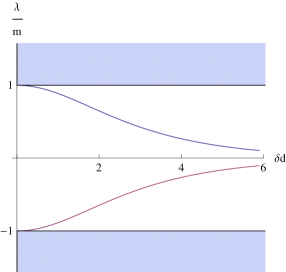
Figure 5: The spectrum of the Hamiltonian (36). The asymptotic twist of the nanotube (40) induces bound states of energies (41). The parameter $m$ is proportional to the inverse of the radius of the nanotube, see scale .

Up to now, the twisted nanotubes were considered to be metallic. The analysis can be extended to semi-conducting nanotubes without any difficulties; a constant, nonzero, part of the vector potential $\tilde{\Delta}_{1}$ has to be associated with the internal characteristics (the orientation of the hexagonal lattice) of the nanotube. Let us notice in this context that the metallic nanotube can be converted into the semi-conducting one just by switching on the constant magnetic flux parallel to the axis of the nanotube. This fact was experimentally confirmed in ABoscillations and coined as Aharonov-Bohm oscillations of the carbon nanotubes. Turning back to (36), we can interpret the Hamiltonian as the energy operator of the semiconducting nanotube with a radial twist associated to $\tilde{\Delta}_{T}$. The constant part $p_{y}\equiv\tilde{\Delta}_{MG}$ of the potential appears due to the semiconducting nature of the nanotube.

V Discussion

The expressions (34) and (38) can be written in the unified form

$$\tilde{\rho}_{I(II)}=\rho_{I(II)}\left(1-\sum_{j}\frac{\sqrt{m^{2}-\lambda_{j}^{2}}}{(\lambda^{2}-\lambda_{j}^{2})}v_{j}^{\dagger}v_{j}\right),$$

where the sum is taken over the normalized bound states of $\tilde{h}_{I(II)}$ annihilated by $L_{I(II)}$. It manifests a decrease of the LDOS in the regions where the bound states are localized. However, it is rather just a peculiar property of the discussed reflectionless models feinbergformule . In general case, the LDOS (27) of $\tilde{h}_{II}$ acquires the following form in terms of the vectors $v_{1}$ and $v_{2}$,

$$\mbox{Tr}(\tilde{G}_{II}(x,x;\lambda)) = \mbox{Tr}({G}_{II}(x,x;\lambda))$$

$$+\frac{2\lambda_{1}^{2}v_{1}^{\dagger}v_{1}\left(g_{0}v_{1}^{\dagger}v_{1}+g_{3}v_{1}^{\dagger}\sigma_{3}v_{1}-g_{1}\frac{\lambda}{\lambda_{1}}v_{1}^{\dagger}\sigma_{1}v_{1}\right)}{(\lambda^{2}-\lambda_{1}^{2})(\det V)^{2}}.$$

When $h_{II}$ is equal to the free particle Hamiltonian, the coefficient of $v_{1}^{\dagger}v_{1}$ reduces to a constant. Nevertheless, this apparently does not hold in the general case.

We restricted our consideration just to the systems described by the Hamiltonian $\tilde{h}=i\sigma_{2}\partial_{x}+\Delta_{1}(x)\sigma_{1}$. However, the potential term of the seed Hamiltonian $h$ in (3) can acquire quite generic form, yet keeping valid the formulas (23) and (25) for the Green’s functions and for the LDOS. Other results are more sensitive to the explicit form of the potential. The term $\Delta_{2}(x)\sigma_{2}$ cannot cause any substantial modifications; it would play just the role of non-physical gauge field. In contrary, impact of the diagonal term $\mathbf{1}\Delta_{0}+\Delta_{3}(x)\sigma_{3}$ in $\tilde{h}$ would be much deeper: in general, it would break the symmetry $\sigma(\tilde{h})=-\sigma(\tilde{h})$ of the spectrum $\sigma(\tilde{h})$ of $\tilde{h}$. In the context of Dirac particles in the carbon nanotubes, the potential $\Delta_{3}(x)\sigma_{3}$ would have different sign for the spin -up and -down components of wave function, i.e. this potential would change the sign on the two sublattices that form the crystal. Physical realization of such a scenario in the considered condensed matter system is not clear. It is remarkable that the Darboux transformation (4) does not alter the form of $\Delta_{0}$; the new Hamiltonian $\tilde{h}$ shares the same electrostatic potential as the seed Hamiltonian. We notice that the electrostatic potential can be also altered via the so-called 0-th order supersymmetry, as it was discussed in nasKlein .

In the discussed systems represented by the stationary equation (1), the analysis of the bound states can be facilitated by the fact that the square of the Dirac Hamiltonian takes the form $-\partial_{x}^{2}+\Delta_{1}^{2}+\sigma_{3}\Delta_{1}^{\prime}$. The existing tools (see, e.g. Schubin ) for the analysis of the Schrödinger operators can be exploited to reveal spectral properties of the Dirac Hamiltonian. In this context, let us mention that interesting results were obtained by the spectral analysis of general class of deformed quantum waveguides described by Schrödinger equation quantumwaveguides . We believe that similar analysis for the carbon nanostructures described by the one- or two-dimensional Dirac Hamiltonian would be fruitful.

The presented analysis is qualitative. The equation (1) is a good approximation for the quasiparticles in carbon nanotubes only for small region of the momentum space where the linear dispersion relation is valid. When the gap opened by the pseudo-magnetic field in the spectrum is too big, nonlinear (the so-called trigonal warping) terms trigonal have to be included into the Hamiltonian. In the article, we neglected surface curvature of the nanotubes. The tubular surface prevents the $\pi$-orbitals of the carbon atoms to be parallel to each other. This implies presence of additional pseudo-magnetic fields in the Hamiltonian. However, in case of armchair nanotubes, these additional gauge fields can be transformed out KaneMele .

The examples presented in the text suggest that the non-uniform radial twist can induce bound states in the nanotube. In particular, the second model with double-kink potential provides an interesting qualitative insight into realistic experimental setting: the nanotube with asymptotically vanishing twist is immersed into the homogeneous magnetic field. Besides the explicit formula (38) for LDOS, the model predicts the appearance of bound states and the formula (41) fixes their energies in dependence on the asymptotic twist. The model can be simply tuned with the use of perturbation techniques.

The supersymmetry can be very useful for construction of the models with more complicated (yet asymptotically constant) twist inducing richer spectral properties. The formalism presented in the second section can be repeated to produce a chain of solvable Hamiltonians, $h$, $\tilde{h}$, $\tilde{\tilde{h}},...$, by taking the last constructed operator as the seed Hamiltonian for the new system. These new solvable systems shall provide insight into the deformation-induced spectral engineering of carbon nanotubes. The reflectionless models are particularly important in this context; they are analytically feasible and possess nontrivial (super)symmetry, analog of (29) and (30). The considered double-kink example suggests that the number of bound states could be in a simple relation to the vector potential of the Hamiltonian; the number of bound states might be proportional to the number of minima of the potential. Verification of this hypothesis goes beyond the scope of the current paper and should be discussed elsewhere.

Acknowledgements:

The work has been partially supported by FONDECYT Grant No. 1095027, Chile, and by the GAČR Grant P203/11/P038, Czech Republic. VJ thanks the Department of Physics of the Universidad de Santiago de Chile for hospitality.

References

-
(1)
G. Başar, G. V. Dunne,
Phys. Rev. Lett. 100, 200404 (2008);
G. Başar, G. V. Dunne, Phys. Rev. D 78, 065022 (2008). - (2) J. Feinberg, Annals Phys. 309, 166 (2004).
- (3) M. Thies, J. Phys. A 39, 12707 (2006).
- (4) R. Jackiw, C. Rebbi, Phys. Rev. D 13, 3398 (1976).
- (5) R. Jackiw, J. R. Schrieffer, Nucl. Phys. B 190, 253, (1981).
- (6) Hajime Takayama, Y. R. Lin-Liu, and Kazumi Maki, Phys. Rev. B 21, 2388 (1980).
- (7) T. L. Ho, J. R. Fulco, J. R. Schrieffer, and F. Wilczek, Phys. Rev. Lett. 52, 1524 (1984).
-
(8)
J. Bar-Sagi, C. G. Kuper, Phys. Rev. Lett. 28, 1556 (1972);
J. Bar-Sagi, C. G. Kuper, J. Low Temp. Phys. 16, 73 (1974). - (9) D. Waxman, G. Williams, Annals Phys. 220, 274 (1992).
- (10) P. R. Wallace, Phys. Rev. 71, 622 (1947).
- (11) G. W. Semenoff, Phys. Rev. Lett. 53, 2449 (1984).
- (12) The Pauli matrices , , are defined in a standard way. Identity matrix is denoted as .
- (13) J. C. Charlier, X. Blase, and S. Roche, Rev. Mod. Phys. 79, 677 (2007).
- (14) C. L. Kane, E. J. Mele, Phys. Rev. Lett. 78, 1932 (1997).
- (15) I. Kosztin, Š. Kos, M. Stone, and A. J. Leggett, Phys. Rev. B 58, 9365 (1998).
- (16) J. Tersoff, D. R. Hamann, Phys. Rev. B 31, 805 (1985).
- (17) Z. F. Wang, Ruoxi Xiang, Q. W. Shi, Jinlong Yang, Xiaoping Wang, J. G. Hou, and Jie Chen, Phys. Rev. B 74, 125417 (2006).
- (18) V. Jakubský, L. M. Nieto, and M. S. Plyushchay, Phys. Rev. D 83, 047702 (2011).
- (19) A. H. Castro Neto, F. Guinea, N. M. R. Peres, K. S. Novoselov, and A. K. Geim, Rev. Mod. Phys. 81, 109 (2009).
- (20) T. Ando, T. Nakanishi, J. Phys. Soc. Jap. 67, 1704 (1998).
- (21) H. Suzuura, T. Ando, Phys. Rev. B 65, 235412 (2002).
- (22) M. A. H. Vozmediano, M. I. Katsnelson and F. Guinea, Phys. Rept. 496, 109 (2010).
-
(23)
A. De Martino, L. Dell’Anna, and R. Egger, Phys. Rev. Lett. 98, 066802 (2007);
Ş. Kuru, J. Negro, and L. M. Nieto, J. Phys.: Condens. Matter 21, 455305 (2009);
R. R. Hartmann, N. J. Robinson, and M. E. Portnoi, Phys. Rev. B 81, 245431 (2010);
E. Milpas, M. Torres, and G. Murguía, J. Phys.: Condens. Matter 23, 245304 (2011). -
(24)
O. Klein,
Z. Phys. 53, 157 (1929);
R. K. Su, G. G. Siu, and X. Chou, J. Phys. A 26, 1001 (1993). - (25) M. I. Katsnelson, K. S. Novoselov, and A. K. Geim, Nature Physics 2, 620 (2006).
-
(26)
G. Junker, Supersymmetric Methods in Quantum and Statistical Physics (Springer, Berlin, 1996);
F. Cooper, A. Khare and U. Sukhatme, Supersymmetry in Quantum Mechanics (Singapore: World Scientific, 2001). - (27) L. M. Nieto, A. A. Pecheritsin, and B. F. Samsonov, Annals Phys. 305, 151 (2003).
- (28) E. N. Economou, Green’s Functions in Quantum Physics, (Springer, 1990).
-
(29)
E. Pozdeeva, J. Phys. A 41, 145208 (2008);
E. Pozdeeva, A. Schulze-Halberg, J. Phys. A 41, 265201 (2008). -
(30)
J. Feinberg,
Phys. Rev. D 51, 4503 (1995);
J. Feinberg and A. Zee, Phys. Rev. D 56, 5050 (1997). -
(31)
B. F. Samsonov, C. V. Sukumar, and A. M. Pupasov, J. Phys. A 38, 7557 (2005);
A. M. Pupasov, B. F. Samsonov, and U. Guenther, J. Phys. A 40, 10557 (2007). - (32) A. Schulze-Halberg, J. Math. Phys. 51, 053501 (2010).
- (33) F. Correa, G. V. Dunne, and M. S. Plyushchay, Annals Phys. 324, 2522 (2009).
-
(34)
F. Correa, M. S. Plyushchay,
Annals Phys. 322, 2493 (2007);
F. Correa, V. Jakubský, L. -M. Nieto, and M. S. Plyushchay, Phys. Rev. Lett. 101, 030403 (2008). - (35) M. S. Plyushchay, L. M. Nieto, Phys. Rev. D 82, 065022 (2010).
- (36) F. Correa, V. Jakubský, and M. S. Plyushchay, Annals Phys. 324, 1078 (2009).
- (37) R. F. Dashen, B. Hasslacher, and A. Neveu, Phys. Rev. D 12, 2443 (1975).
- (38) A. Bachtold et.al, Nature 397, 673 (1999).
- (39) Similar formula was found in Feinberg for the reflectionless models by the inverse scattering method.
- (40) F. A. Berezin, M. Shubin, The Schrödinger Equation, (Springer 1991).
-
(41)
P. Duclos, P. Exner, Rev. Mat. Phys. 7, 73 (1995);
T. Ekholm, H. Kovařík, and D. Krejčiřík, Arch. Ration. Mech. Anal. 188, 245 (2008);
D. Krejčiřík, Analysis on Graphs and Its Applications, Proceedings of Symposia in Pure Mathematics Vol. 77, (American Mathematical Society, Providence, Rhode Island, 2008), p. 617 and references therein. -
(42)
T. Ando, T. Nakanishi, and R. Saito, J. Phys. Soc. Jpn. 67, 2857 (1998);
R. Saito, G. Dresselhaus, and M. S. Dresselhaus, Phys. Rev. B 61, 2981 (2000). - (43) Equation (1) is the approximation of the tight-binding model for energies that are close to the selected Dirac point (i.e. ). In the tight-binding model of the nanotubes Roche , nasKlein , the mass (or the external field) parameter is in the fixed relation to the radius of the nanotube. The quantized momenta form equidistant lines with mutual distance in the first Brioullin zone. In case of the metallic nanotubes, one of the lines passes through the considered Dirac point when no external field is present. The external field associated with induces the spectral gap by shifting this line into the distance from the Dirac point. Hence, corresponds to a fixed fraction of the distance between the lines. Recovering the relevant constants, we get and , ando . Here is hopping parameter (), the lattice constant and is dependent on the external field. For , the system is equivalent to a semi-conducting nanotube in absence of the external field Roche .