The BFKL Pomeron calculus: summing enhanced diagrams

Abstract:

The goal of this paper is to sum over a class of enhanced diagrams, and derive a new Pomeron Green function. It is found that this sum gives the Pomeron contribution to the scattering amplitude that decreases with energy. In other words, we found that the total cross section of two colourless dipoles of small but equal sizes, falls down at high energies.

1 Introduction

High energy QCD has reached a mature stage of development, for dilute-dense scattering (for example for DIS with nuclei) [1, 2, 3, 4, 5, 6]. However, for dilute-dilute scattering at high energy, (for example the scattering of two virtual photons with large but almost equal virtualities), despite the great deal of effort by experts in the field (see for example Refs. [7, 8, 9, 10, 11, 12, 13, 14, 15] ), we are still waiting for the desired breakthrough. In this paper we address the problem of the scattering amplitude for the dilute - dilute system, using the BFKL Pomeron calculus [16, 30, 1, 2, 12, 16, 17]. The BFKL Pomeron calculus is elegantly formulated in terms of the functional integral [12]. Namely,

$$Z[\Phi,\Phi^{+}]\,\,=\,\,\int\,\,D\Phi\,D\Phi^{+}\,e^{S}\,\,\,\hskip 14.22636pt\mbox{with}\hskip 14.22636pt\,S\,=\,S_{0}\,+\,S_{I}\,+\,S_{E}$$ (1.1)

where $S_{0}$ describes free Pomerons, $S_{I}$ corresponds to their mutual interaction while $S_{E}$ relates to the interaction with the external sources (target and projectile). $S_{0}$ has a simple expression:

$$S_{0}\,=\,\int\,dY\,dY^{\prime}\,d^{2}x_{1}\,d^{2}x_{2}\,d^{2}x^{\prime}_{1}\,d^{2}x^{\prime}_{2}\,\Phi^{+}(x_{1},x_{2};Y)\,G^{-1}(x_{1},x_{2};Y|x^{\prime}_{1},x^{\prime}_{2};Y^{\prime})\,\Phi(x^{\prime}_{1},x^{\prime}_{2};Y^{\prime})$$ (1.2)

while

$$S_{I}\,=\,\frac{2\,\pi\bar{\alpha}_{s}^{2}}{N_{c}}\,\int\,dY^{\prime}\,\int\,\frac{d^{2}x_{1}\,d^{2}x_{2}\,d^{2}x_{3}}{x^{2}_{12}\,x^{2}_{23}\,x^{2}_{13}}\Big{\{}\left(L_{12}\Phi(x_{1},x_{2};Y^{\prime})\,\right)\,\Phi^{+}(x_{1},x_{3};Y^{\prime})\,\Phi^{+}(x_{3},x_{2};Y^{\prime})\,\,+\,\,h.c.\Big{\}}$$ (1.3)

where $h.c.$ denotes the Hermitian conjugate. $S_{E}$ describes the interaction with the scattering particles (two small colliding dipoles in our case), but we do not need the explicit expression for this term in our paper. $Y$ is the rapidity of the dipole. For dipole-dipole scattering $Y=\ln s$ in the leading log approximation where $s$ is the energy of colliding dipoles. Eq. (1.1) is written in the leading log approximation. The following notation, $\bar{\alpha}_{s}=N_{c}\alpha_{s}/\pi$ will be assumed throughout. $\Phi$ and $\Phi^{+}$ relate to the BFKL Pomeron and $G(x_{1},x_{2};Y|x^{\prime}_{1},x^{\prime}_{2};Y^{\prime})$ is the Green function of the BFKL Pomeron which takes the form:

$$G^{-1}(x_{1},x_{2};Y|x^{\prime}_{1},x^{\prime}_{2};Y^{\prime})\hskip 8.5359pt=\hskip 8.5359ptp^{2}_{1}\,p^{2}_{2}\,\left(\frac{\partial}{\partial Y}+H\right)\hskip 8.5359pt=\hskip 8.5359pt\left(\frac{\partial}{\partial Y}+H^{+}\right)\,p^{2}_{1}\,p^{2}_{2}$$ (1.4)

with

$$Hf(x_{1},x_{2};Y)\,\,=\,\,\frac{\bar{\alpha}_{s}}{2\pi}\,\int\,d^{2}x_{3}\,K\left(x_{1},x_{2}|x_{3}\right)\,\left\{f(x_{1},x_{2};Y)\,-\,f(x_{1},x_{3};Y)\,-\,f(x_{3},x_{2};Y)\right\}$$ (1.5)

where

$$K\left(x_{1},x_{2}|x_{3}\right)\hskip 8.5359pt=\hskip 8.5359pt\frac{x^{2}_{12}}{x^{2}_{23}\,x^{2}_{13}}\hskip 56.9055ptL_{12}\hskip 8.5359pt=\hskip 8.5359ptx^{4}_{12}\,p^{2}_{1}\,p^{2}_{2}\hskip 56.9055ptp_{k}\hskip 8.5359pt=\hskip 8.5359pt-i\nabla_{x_{k}}\hskip 14.22636pt\left(k\,=\,1,2\right)$$ (1.6)

The exact Green function for the Pomeron, which is the goal of this paper to derive, is equal to:

$$G(x_{1},x_{2};Y|x^{\prime}_{1},x^{\prime}_{2};Y^{\prime})\,\,=\,-\frac{\int D\Phi\,D\Phi^{+}\Phi\left(x_{1},x_{2};Y\right)\,\Phi^{+}\left(x^{\prime}_{1}.x^{\prime}_{2};Y^{\prime}\right)\,e^{S[\Phi,\Phi^{+}]}}{\int D\Phi\,D\Phi^{+}\,e^{S[\Phi,\Phi^{+}]}}$$ (1.7)

and the bare (initial) BFKL Pomeron Green function[30] is determined by Eq. (1.7), where only the term $S_{0}$ is included in $S[\Phi,\Phi^{+}]$.

It is worthwhile mentioning that due to conformal invariance of the BFKL Pomeron calculus, the form of the triple Pomeron vertex is known unambiguously, and coincides with the direct calculations found in ref. [17] The simplicity of Eq. (1.1) is thanks to the key assumption, that the triple Pomeron vertex is the only essential vertex for Pomeron interactions. In other words. in Eq. (1.1) we neglect all other local vertices (for example, the vertex for the transition of one Pomeron to three and so on). We have no rigorous proof for this conjecture. There even exist arguments that the four Pomeron vertex should also be included [18]. It should noted also, that the BFKL Pomeron calculus given by Eq. (1.1), is formulated in the leading $1/N_{c}$ approximation, where $N_{c}$ is the number of colours. It is known that the BFKL Pomeron calculus cannot be a correct approximation for the scattering amplitude in the next-to-leading order in $1/N_{c}$ approach, due to the fact that $2n$- gluon states in the $t$-channel give a larger intercept than $n$ BFKL Pomerons [19]. Nevertheless we consider Eq. (1.1) to be a good first approximation, for the dilute-dilute system of scattering. We will return to the discussion of all these problems in the conclusion, where we show that they are not important for the solution derived in this paper.

The goal of this paper is to calculate the class of enhanced diagrams. The simplest examples of these diagrams are shown in Fig. 2 and Fig. 5. In other words we are going to sum BFKL Pomeron loops in this paper. These diagrams lead to a new Green function of the BFKL Pomeron (the term $S_{0}$ in Eq. (1.1) ), while the vertices of the interaction of the new dressed Pomeron remain the same as they appear in $S_{I}$. It is worthwhile mentioning that if the Green function of the dressed Pomeron, will be such that the Pomeron contribution will lead to a decrease with energy, then the problem would be solved without needing to consider the interaction of the dressed Pomerons. However, if this is not the case and the dressed Pomeron still increases with energy, then the interaction of the dressed Pomeron needs to be included. On the other hand, for the scattering of two dipoles with small sizes, within a wide range of energy the enhanced diagrams dominate, since the interactions of the Pomeron with the target and the projectile are small in the leading $1/N_{c}$-approximation.

This paper is organized in the following way. In the next section the formulae for the triple Pomeron vertex and the Pomeron Green function are introduced. Using these ingredients we calculate the sum over the class of enhanced diagrams shown in Fig. 2 - Fig. 5, namely one-Pomeron loops in series, in $\left(\omega,\nu\right)$ representation. This is done in a step-by-step way, in order to introduce the reader to the method of integration and assumptions used in this treatment, which will be used later on for more complicated diagrams.

The third section is the main body of this paper. Using the techniques developed in section 2, we extend this approach to the sum over all enhanced diagrams, using two principle selection rules. First, we are searching only for the contribution to the vertices that are singular in $\nu$. Second, we assume that the contribution of the Pomeron loops in effective vertices, for multi-Pomeron production are negligibly small. This approximation is closely related to the Mueller-Patel-Salam-Iancu approach [20], but in this paper this strategy is formulated in $(\omega,\nu)$-representation. In section 3.1 the equations for the effective multi-Pomeron vertices are derived and solved. In section 3.2 we present the results of the summation, for the Green function of the dressed Pomeron. It turns out that the exchange of the dressed Pomeron, leads to the total cross section for dipole-dipole scattering that decreases with energy. This result is reminiscent of the Pomeron Green function in $1+1$ dimensional Pomeron calculus, [21, 22, 23, 24, 25] which also decreases due to the contribution of Pomeron loops. In the conclusion section, we summarize our results, and discuss the current stage of development of the BFKL Pomeron calculus. The appendix provides detailed information about the ingredients of the BFKL Pomeron calculus, including the bare Pomeron Green function and the triple Pomeron vertex.

2 Summing simple Pomeron loops

In this section we sum the set of enhanced diagrams shown in Fig. 2 - Fig. 5, namely one-Pomeron loops in series. The sum over all diagrams of this type will teach us the main characteristic features of the enhanced diagrams, which we will use for developing an approach for summing over a more general class of diagrams.

2.1 Bare Pomeron

Figure 1: The basic diagram with the exchange of one Pomeron in the $t$-channel.

Figure 2: The diagram with one Pomeron loop.

The most basic diagram is the exchange of one Pomeron in the $t$-channel without any loops. The expression for this diagram which is shown in Fig. 2 is given by the following expression in $\omega$ representation [26, 27, 35, 28, 29]:

$$G_{0}\left(\omega,\nu\right)\hskip 8.5359pt=\hskip 8.5359pt\,\frac{g\left(\nu\right)}{\omega-\omega\left(\nu\right)}\,\,\,\,\,\,\,\,\,\,\,\,\,\mbox{where}\hskip 14.22636ptg\left(\nu\right)\hskip 8.5359pt=\hskip 8.5359pt\frac{\nu^{2}}{\biggl{(}\nu^{2}+{\frac{1}{4}}\biggr{)}^{2}}$$ (2.8)

The following inverse Mellin transform allows us to pass to $Y$ representation:

$$G_{0}\left(Y,\nu\right)\hskip 8.5359pt=\hskip 8.5359pt\frac{1}{2\pi i}{{\int}}^{a+i\infty}_{a-i\infty}d\omega\,\,\,e^{\omega\,Y}G_{(0)}\left(\omega,\nu\right)\hskip 8.5359pt=\hskip 8.5359pt\,e^{\,\omega\left(\nu\right)\,Y}\,g\left(\nu\right)\,$$ (2.9)

The contour of integration is placed to the right of all singularities of $G_{0}\left(\omega,\nu\right)$.

2.2 One loop

The first correction to the basic diagram is the diagram with one loop shown below in Fig. 2. The amplitude for the one-loop diagram takes the following form in $\omega$ representation [12]:

$$A_{(1)}\left(\omega,\nu\right)\hskip 8.5359pt=\hskip 8.5359ptG_{0}\left(\omega,\nu\right){{\int}}^{\infty}_{-\infty}\!\!d\nu^{\,\prime}\,\,m\left(\omega,\nu,\nu^{\,\prime}\right)G_{0}\left(\omega,\nu^{\,\prime}\right)$$ (2.10)

where $m\left(\nu,\nu^{\,\prime},\omega\right)$ is the Pomeron self mass, given by the following formula:

$$m\left(\nu,\nu^{\,\prime},\omega\right)\hskip 8.5359pt=\hskip 8.5359pt\,{{\int}}^{\infty}_{-\infty}d\nu_{1}\,{{\int}}^{\infty}_{-\infty}d\nu_{2}\,g\left(\nu_{1}\right)\,g\left(\nu_{2}\right){\frac{\Gamma\biggl{(}\nu\,\begin{vmatrix}\,\nu_{1},\nu_{2}\biggr{)}\Gamma\biggl{(}\nu^{\,\prime}\,\end{vmatrix}\,\nu_{1},\nu_{2}\biggr{)}}{\biggl{(}\,\omega-\omega\left(\nu_{1}\right)-\omega\left(\nu_{2}\right)\,\biggr{)}}}\hskip 28.45274pt$$ (2.11)

The triple Pomeron vertex has the following definition [34] :

$$\Gamma\left(\nu\,|\,\nu_{1},\nu_{2}\right)\hskip 8.5359pt=\hskip 8.5359pt\frac{16\,\bar{\alpha}_{s}^{2}}{N_{c}}\left(\Gamma_{\mbox{\footnotesize{planar}}}\left(\nu\,|\,\nu_{1},\nu_{2}\right)-\frac{2\pi}{N_{c}^{2}}\,\,\Gamma_{\mbox{\footnotesize{non-planar}}}\left(\nu\,|\,\nu_{1},\nu_{2}\right)\right)$$ (2.12)

$$\Gamma_{\mbox{\footnotesize{planar}}}\left(\nu\,|\,\nu_{1},\nu_{2}\right)\hskip 8.5359pt=\hskip 8.5359pt\left({\frac{1}{4}}+\nu^{2}\right)^{2}\Omega\left(\nu\,|\,\nu_{1},\nu_{2}\right)$$ (2.13)

$$\Gamma_{\mbox{\footnotesize{nonplanar}}}\left(\nu\,|\,\nu_{1},\nu_{2}\right)\hskip 8.5359pt=\hskip 8.5359pt\left({\frac{1}{4}}+\nu^{2}\right)^{2}\Lambda\left(\nu\,|\,\nu_{1},\nu_{2}\right)\biggl{(}\chi\left(\nu\right)-\chi\left(\nu_{1}\right)-\chi\left(\nu_{2}\right)\biggr{)}$$ (2.14)

where the functions $\chi\left(\nu\right)$ , $\,\,\Omega\left(\nu\,|\,\nu_{1},\nu_{2}\right)$ and $\Lambda\left(\nu\,|\,\nu_{1},\nu_{2}\right)$ are defined explicitly in Eqs. (A.2), (A.6) and (A.24) respectively. $\Gamma_{\mbox{\footnotesize{planar}}}$ and $\Gamma_{\mbox{\footnotesize{nonplanar}}}$ denote the two diagrams that contribute to the vertex, namely the planar and non-planar diagrams shown below in Fig. 3 (a) and Fig. 3 (b) (the diagrams in Fig. 3 are taken from ref. [34]).

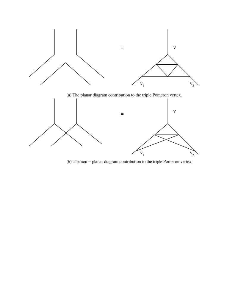
Figure 3: The two contributing diagrams to the triple Pomeron vertex.

$\Gamma\left(\nu\,|\,\nu_{1},\nu_{2}\right)$ is the vertex at the top of the loop of Fig. 2, whereby the Pomeron with scaling dimension $\nu$ splits into two Pomerons that form the loop, with scaling dimensions $\nu_{1}$ and $\nu_{2}$. The vertex at the bottom of the loop is labeled by $\Gamma\left(\nu^{\,\prime}\,|\,\nu_{1},\nu_{2}\right)$, whereby the Pomerons with scaling dimensions $\nu_{1}$ and $\nu_{2}$ recombine to one Pomeron with scaling dimension $\nu^{\,\prime}$. Before proceeding to calculate $m\left(\omega,\nu,\nu^{\,\prime}\right)$, it is instructive to switch to the variables $\lambda$, $\sigma$ and $\Delta$ defined as:

$$\lambda\hskip 8.5359pt=\hskip 8.5359pti/2-\nu\,;\hskip 28.45274pt\lambda^{\,\prime}\hskip 8.5359pt=\hskip 8.5359pti/2-\nu^{\,\prime}\,;\hskip 28.45274pt\sigma\hskip 8.5359pt=\hskip 8.5359pt\nu_{1}+\nu_{2}\,;\hskip 28.45274pt\Delta\hskip 8.5359pt=\hskip 8.5359pt\nu_{1}-\nu_{2}$$ (2.15)

In tems of ($\lambda,\sigma,\Delta$) variables, then Eq. (2.11) reads:

$$m\left(\omega,\lambda,\lambda^{\,\prime}\right)\hskip 8.5359pt=\hskip 8.5359pt{{\int}}^{\infty}_{-\infty}d\sigma{{\int}}^{\infty}_{-\infty}d\Delta\,\,g\left({\frac{\sigma+\Delta}{2}}\right)g\left({\frac{\sigma-\Delta}{2}}\right)\frac{\Gamma\biggl{(}\lambda\,\begin{vmatrix}\,\sigma,\Delta\biggr{)}\Gamma\biggl{(}\lambda^{\,\prime}\,\end{vmatrix}\,\sigma,\Delta\biggr{)}}{\left(\,\omega-\omega\left({\frac{\sigma+\Delta}{2}}\right)-\omega\left({\frac{\sigma-\Delta}{2}}\right)\,\right)}\,\,\hskip 28.45274pt$$ (2.16)

The product of vertices $\Gamma\left(\lambda\,|\,\sigma,\Delta\right)\Gamma\left(\lambda^{\,\prime}\,|\,\sigma,\Delta\right)$ that appears in Eq. (2.16), contains two poles in the $\sigma$-plane in the following regions (for details see Eqs. (A.16 - A.18) and Eq. (A.24)):

$$\sigma\hskip 8.5359pt=\hskip 8.5359pt\lambda\hskip 45.52458pt\Leftrightarrow\hskip 28.45274pti/2-\nu\hskip 8.5359pt=\hskip 8.5359pt\nu_{1}+\nu_{2}$$ (2.17)

$$\sigma\hskip 8.5359pt=\hskip 8.5359pti-\lambda\hskip 28.45274pt\Leftrightarrow\hskip 28.45274pti/2+\nu\hskip 8.5359pt=\hskip 8.5359pt\nu_{1}+\nu_{2}$$ (2.18)

We need to check that the vertices $\Omega$ and $\Lambda$ converge as $\nu\to\infty$, for both of the regions of Eq. (2.17) and Eq. (2.18). From Eq. (A.24) its clear that $\Lambda$ falls down for pure imaginary $\nu=i\kappa$, as $\exp\left(-2\,\kappa\ln\kappa\right)$. Actually, we will see below that we need to integrate the $\nu$-image of the amplitude to calculate the scattering amplitude in coordinate space, in the following way:

$$A\left(\zeta\right)\,\,=\,\,\int\frac{d\nu}{2\pi}\,e^{i\nu\ln\zeta}\,A\left(\nu\right)$$ (2.19)

One can see, that independent from the sign of $\ln\zeta$, we have to close the $\nu$-contour of integration for $\Lambda$ over the upper half-plane. Since the pole of Eq. (2.17) lies in the upper half-plane, then the $\nu$-integral for the part of the vertex proportional to $\Lambda$, is taken using the contour which is closed around the pole given by Eq. (2.17).

The situation with the part of the vertex proportional to $\Omega$ is quite different. One can see that at large and pure imaginary $\nu$, then $\Omega$ falls down only as a power of $\nu$. Therefore, the convergence of the integral in Eq. (2.19) depends on the sign of $\ln\zeta$. We choose $\zeta>1$ . For this choice of $\zeta$ we can close the $\nu$-integration contour over the upper half-plane for both $\Lambda$ and $\Omega$.

With this in mind, $\lambda\to 0$ from above the real axis, is our region of interest for calculating the contribution to the vertex proportional to $\Lambda$. Whereas $\lambda\to 0$ from below the real axis, is the relevant region for calculating the part of the vertex proportional to $\Omega$. The dominant high energy behaviour $\exp\left(2\omega_{0}\,Y\right)$ stems from the region $\nu_{1},\nu_{2}\to 0$, (or in other words $\sigma\to 0$). Thus since $\lambda\to 0^{+}$ is our region of interest, then Eq. (2.17) is the relevant region, whereas Eq. (2.18) does not yield $\sigma\to 0$ as $\lambda\to 0^{+}$. In light of this observation, it is useful to extract the pole explicitly by making the following definition:

$$\Gamma\left(\lambda\,|\,\sigma,\Delta\right)\hskip 8.5359pt=\hskip 8.5359pt{\frac{\tilde{\Gamma}\left(\lambda\,|\,\sigma,\Delta\right)}{\lambda-\sigma}}$$ (2.20)

In this approach, $\tilde{\Gamma}\left(\lambda\,|\,\sigma,\Delta\right)$ is finite in the region $\sigma\to\lambda$. Hence plugging Eq. (2.20) into Eq. (2.16) leads to the following formula:

$$m\left(\omega,\lambda,\lambda^{\,\prime}\right)\hskip 8.5359pt=\hskip 8.5359pt{{\int}}^{\infty}_{-\infty}d\sigma{{\int}}^{\infty}_{-\infty}d\Delta\,\,\,\frac{g\left({\frac{\sigma+\Delta}{2}}\right)g\left({\frac{\sigma-\Delta}{2}}\right)}{\left(\,\omega-\omega\left({\frac{\sigma+\Delta}{2}}\right)-\omega\left({\frac{\sigma-\Delta}{2}}\right)\,\right)}\,\,\frac{\tilde{\Gamma}\biggl{(}\lambda\,\begin{vmatrix}\,\sigma,\Delta\biggr{)}\tilde{\Gamma}\biggl{(}\lambda^{\,\prime}\,\end{vmatrix}\,\sigma,\Delta\biggr{)}}{\biggl{(}\lambda-\sigma\biggr{)}\biggl{(}\lambda^{\,\prime}-\sigma\biggr{)}}\hskip 28.45274pt$$ (2.21)

$$=\hskip 8.5359pt-2\pi i{{\int}}^{\infty}_{-\infty}d\Delta\,\,\left\{\,\frac{g\left({\frac{\sigma+\Delta}{2}}\right)g\left({\frac{\sigma-\Delta}{2}}\right)}{\left(\,\omega-\omega\left({\frac{\sigma+\Delta}{2}}\right)-\omega\left({\frac{\sigma-\Delta}{2}}\right)\,\right)}\,\,\frac{\tilde{\Gamma}\biggl{(}\lambda\,\begin{vmatrix}\,\sigma,\Delta\biggr{)}\tilde{\Gamma}\biggl{(}\lambda^{\,\prime}\,\end{vmatrix}\,\sigma,\Delta\biggr{)}}{\biggl{(}\lambda^{\,\prime}-\lambda\biggr{)}}\,\,\right\}_{\sigma\,=\,\lambda}\hskip 28.45274pt$$ (2.22)

where in the last step the $\sigma$-integral was solved by taking the residue of the pole at $\sigma\hskip 8.5359pt=\hskip 8.5359pt\lambda$. Switching back to $\left(\nu,\nu_{1},\nu_{2}\right)$ variables, then Eq. (2.22) reads:

$$m\left(\omega,\nu,\nu^{\,\prime}\right)\hskip 8.5359pt=\hskip 8.5359pt-2\pi i{{\int}}^{\infty}_{-\infty}d\nu_{2}\left\{\frac{g\left(\nu_{1}\right)g\left(\nu_{2}\right)}{\biggl{(}\omega-\omega\left(\nu_{1}\right)-\omega\left(\nu_{2}\right)\biggr{)}}\,\,\frac{\tilde{\Gamma}\biggl{(}\nu\,\begin{vmatrix}\,\nu_{1},\nu_{2}\biggr{)}\tilde{\Gamma}\biggl{(}\nu^{\,\prime}\,\end{vmatrix}\,\nu_{1},\nu_{2}\biggr{)}}{\biggl{(}\nu^{\,\prime}-\nu\biggr{)}}\right\}_{i/2-\nu\,=\,\nu_{1}+\nu_{2}}$$ (2.23)

Interestingly, the Pomeron self-mass $m\left(\omega,\nu,\nu^{\,\prime}\right)$ contains a simple (first order) pole in the region $\nu=\nu^{\,\prime}$. Hence using the result of Eq. (2.23):

$${{\int}}^{\infty}_{-\infty}d\nu^{\,\prime}m\left(\omega,\nu,\nu^{\,\prime}\right)G_{0}\left(\omega,\nu^{\,\prime}\right)=4\pi^{2}{{\int}}^{\infty}_{-\infty}d\nu_{2}\left\{\frac{g\left(\nu_{1}\right)g\left(\nu_{2}\right)\,\tilde{\Gamma}^{2}\biggl{(}\nu\,|\,\nu_{1},\nu_{2}\biggr{)}}{\biggl{(}\omega-\omega\left(\nu_{1}\right)-\omega\left(\nu_{2}\right)\biggr{)}}\,G_{0}\left(\omega,\nu\right)\right\}_{\!i/2-\nu\,=\,\nu_{1}+\nu_{2}}\,\hskip 14.22636pt$$ (2.24)

where the right hand side of Eq. (2.24) was derived by taking the residue of the pole at $\nu\,=\,\nu^{\,\prime}$, after integrating over $\nu^{\,\prime}$. The right hand side of Eq. (2.24) can be re-written in the following equivalent form:

$${{\int}}^{\infty}_{-\infty}d\nu^{\,\prime}m\left(\omega,\nu,\nu^{\,\prime}\right)G_{0}\left(\omega,\nu^{\,\prime}\right)\hskip 8.5359pt=\hskip 8.5359pt\Sigma\left(\omega,\nu\right)G_{0}\left(\omega,\nu\right)$$ (2.25)

$$\Sigma\left(\omega,\nu\right)\hskip 8.5359pt=\hskip 8.5359pt{{\int}}^{\infty}_{-\infty}d\nu_{1}\,{{\int}}^{\infty}_{-\infty}d\nu_{2}\,\,{\frac{g\left(\nu_{1}\right)\,g\left(\nu_{2}\right)}{\biggl{(}\,\omega-\omega\left(\nu_{1}\right)-\omega\left(\nu_{2}\right)\,\biggr{)}}}\,\frac{\tilde{\Gamma}^{2}\biggl{(}\nu\,|\,\nu_{1},\nu_{2}\biggr{)}}{\left({\frac{i}{2}}-\nu-\nu_{1}-\nu_{2}\right)\,}\,\,$$ (2.26)

where the $\nu_{1}$ integral in Eq. (2.26) is solved by taking the residue of the pole at $i/2-\nu-\nu_{1}-\nu_{2}=0$. Thanks to the simplification of Eq. (2.25), then Eq. (2.10) can be re-cast as:

$$A_{(1)}\left(\omega,\nu\right)\hskip 8.5359pt=\hskip 8.5359ptG_{0}\left(\omega,\nu\right)\Sigma\left(\omega,\nu\right)\,\,G_{0}\left(\omega,\nu\right)$$ (2.27)

In order to pass to $Y$ representation, use the following inverse Mellin transform:

$$A_{(1)}\left(Y,\nu\right)\hskip 8.5359pt=\hskip 8.5359pt\frac{1}{2\pi i}{{\int}}^{a+i\infty}_{a-i\infty}d\omega\,\,\,e^{\omega\,Y}A_{(1)}\left(\omega,\nu\right)$$ (2.28)

which after inserting Eq. (2.27) yields:

$$A_{(1)}\left(Y,\nu\right)\hskip 8.5359pt=\hskip 8.5359pt\,\,g^{2}\left(\nu\right){{\int}}^{\infty}_{-\infty}d\nu_{1}\,{{\int}}^{\infty}_{-\infty}d\nu_{2}\,\frac{g\left(\nu_{1}\right)g\left(\nu_{2}\right)}{\biggl{(}\omega-\omega\left(\nu_{1}\right)-\omega\left(\nu_{2}\right)\biggr{)}}\frac{\tilde{\Gamma}^{2}\biggl{(}\nu\,|\,\nu_{1},\nu_{2}\biggr{)}}{\left({\frac{i}{2}}-\nu-\nu_{1}-\nu_{2}\right)\,}\hskip 28.45274pt$$ (2.29)

$$\times\,{\frac{e^{\omega\left(\nu\right)\,Y}}{\omega\left(\nu\right)-\omega\left(\nu_{1}\right)-\omega\left(\nu_{2}\right)}}\,\left(\,{\frac{e^{\left\{\,\omega\left(\nu_{1}\right)+\omega\left(\nu_{2}\right)-\omega\left(\nu\right)\,\right\}\,Y}\,-1\,}{\omega\left(\nu\right)-\omega\left(\nu_{1}\right)-\omega\left(\nu_{2}\right)}}\,+Y\,\right)$$

2.3 Two loops

Figure 4: The diagram with two Pomeron loops.

Figure 5: The diagram with $n$ Pomeron loops in succession.

The second correction to the basic diagram is the diagram with two loops shown below in Fig. 5. The amplitude for the 2-loop diagram takes the following form in $\omega$ representation:

$$A_{(2)}\left(\omega,\nu\right)\hskip 8.5359pt=\hskip 8.5359ptG_{0}\left(\omega,\nu\right){{\int}}^{\infty}_{-\infty}d\nu^{\,\prime}{{\int}}^{\infty}_{-\infty}d\nu^{\,\prime\prime}\,\,m\left(\omega,\nu,\nu^{\,\prime}\right)\,\,G_{0}\left(\omega,\nu^{\,\prime}\right)\,\,m\left(\omega,\nu^{\,\prime},\nu^{\,\prime\prime}\right)\,\,G_{0}\left(\omega,\nu^{\,\prime\prime}\right)\hskip 28.45274pt$$ (2.30)

Thanks to the useful result of Eq. (2.25), the amplitude for the 2-loop diagram of Eq. (2.30) simplifies to the following formula:

$$A_{(2)}\left(\omega,\nu\right)\hskip 8.5359pt=\hskip 8.5359ptG_{0}\left(\omega,\nu\right)\,\,\biggl{(}\,\,G_{0}\left(\omega,\nu\right)\,\,\Sigma\left(\omega,\nu\right)\,\,\biggr{)}^{2}$$ (2.31)

where $\Sigma\left(\omega,\nu\right)$ is given by Eq. (2.26). In order to pass to $Y$ representation, use the following inverse Mellin transform:

$$A_{(2)}\left(Y,\nu\right)\hskip 8.5359pt=\hskip 8.5359pt\frac{1}{2\pi i}{{\int}}^{a+i\infty}_{a-i\infty}d\omega\,\,\,e^{\omega\,Y}A_{(2)}\left(\omega,\nu\right)\,\,\,$$ (2.32)

$$=\hskip 8.5359ptg^{3}\left(\nu\right)\prod^{2}_{k=1}\,\,\,{{\int}}^{\infty}_{-\infty}d\nu^{k}_{1}\,{{\int}}^{\infty}_{-\infty}d\nu^{k}_{2}\,\,\,g\left(\nu^{k}_{1}\right)\,g\left(\nu^{k}_{2}\right)\frac{\tilde{\Gamma}^{2}\biggl{(}\nu\,|\,\nu^{k}_{1},\nu^{k}_{2}\biggr{)}}{\left({\frac{i}{2}}-\nu-\nu^{k}_{1}-\nu^{k}_{2}\right)\,}$$ (2.33)

$$\times\hskip 8.5359pt\left\{\hskip 8.5359pt{\frac{e^{\omega_{1}\,Y}}{\omega-\omega_{1}}}+{\frac{e^{\omega_{2}\,Y}}{\omega-\omega_{2}}}+e^{\omega\left(\nu\right)\,Y}\left({\frac{1}{\left(\omega-\omega_{1}\right)\left(\omega-\omega_{2}\right)}}\right)\,\frac{1}{2!}\right.$$

$$\left.\hskip 19.91684pt+\hskip 8.5359pte^{\omega\left(\nu\right)\,Y}\frac{d}{d\omega}\left({\frac{1}{\left(\omega-\omega_{1}\right)\left(\omega-\omega_{2}\right)}}\right)\,Y+e^{\omega\left(\nu\right)\,Y}\frac{d^{2}}{d\omega^{2}}\left({\frac{1}{\left(\omega-\omega_{1}\right)\left(\omega-\omega_{2}\right)}}\right)\frac{Y^{2}}{2!}\hskip 8.5359pt\right\}_{\omega\,=\,\omega(\nu)}$$

$$\omega_{k}\hskip 8.5359pt=\hskip 8.5359pt\omega\left(\nu_{1}^{k}\right)+\omega\left(\nu_{2}^{k}\right)$$ (2.34)

2.4 $n$ loops

Extending this approach to the diagram with $n$ loops in succession shown in Fig. 5, leads to the following amplitude in $\omega$ representation:

$$A_{(n)}\left(\omega,\nu\right)\hskip 8.5359pt=\hskip 8.5359ptG_{0}\left(\omega,\nu\right)\,\,\biggl{(}\,\,G_{0}\left(\omega,\nu\right)\,\Sigma\left(\omega,\nu\right)\,\,\biggr{)}^{n}$$ (2.35)

The sum over the class of diagrams shown in Fig. 5 with an alternating minus sign, for all $n\in\left(0,\infty\right)$ i.e. from $n=0$ loops up to infinity gives the Green function of the dressed Pomeron, labeled $G_{2}\left(\omega,\nu\right)$. In this notation:

$$G_{2}\left(\omega,\nu\right)\hskip 8.5359pt=\hskip 8.5359pt\sum^{\infty}_{n=0}\left(-1\right)^{n}A_{(n)}\left(\omega,\nu\right)\,\,\,=\hskip 8.5359pt\frac{G_{0}\left(\omega,\nu\right)}{\biggl{(}\hskip 5.69046pt1\,\,+\,\,G_{0}\left(\omega,\nu\right)\,\Sigma\left(\omega,\nu\right)\,\,\hskip 5.69046pt\biggr{)}}$$ (2.36)

From Eq. (2.36), the renormalized propagator $G_{2}\left(\omega,\nu\right)$ can be expressed in terms of the bare Pomeron propagator $G_{0}\left(\omega,\nu\right)$ as:

$$G_{2}^{-1}\left(\omega,\nu\right)\hskip 8.5359pt=\hskip 8.5359ptG_{0}^{-1}\left(\omega,\nu\right)\hskip 8.5359pt+\hskip 8.5359pt\Sigma\left(\omega,\nu\right)$$ (2.37)

2.5 Calculation of $\Sigma\left(\omega,\nu\right)$

In this section, we calculate explicitly the formula for the Pomeron loop $\Sigma\left(\omega,\nu\right)$, defined above in Eq. (2.26) . In ($\lambda,\sigma,\Delta$) notation introduced in Eqs. (2.15):

$$\Sigma\left(\omega,\lambda\right)\hskip 8.5359pt=\hskip 8.5359pt{{\int}}^{\infty}_{-\infty}d\sigma{{\int}}^{\infty}_{-\infty}d\Delta\,\,\,\frac{g\left({\frac{\sigma+\Delta}{2}}\right)g\left({\frac{\sigma-\Delta}{2}}\right)}{\left(\,\,\,\omega-\omega\left({\frac{\sigma+\Delta}{2}}\right)-\omega\left({\frac{\sigma-\Delta}{2}}\right)\,\,\,\right)}\,\,\frac{\tilde{\Gamma}^{2}\biggl{(}\lambda\,|\,\sigma,\Delta\biggr{)}}{\biggl{(}\lambda-\sigma\biggr{)}}$$ (2.38)

$$=\hskip 8.5359pt-2\pi i\hskip 8.5359pt{{\lim_{\sigma\to\lambda}}}\hskip 8.5359pt{{\int}}^{\infty}_{-\infty}d\Delta\,\,\,\frac{g\left({\frac{\lambda+\Delta}{2}}\right)g\left({\frac{\lambda-\Delta}{2}}\right)}{\left(\,\,\,\omega-\omega\left({\frac{\lambda+\Delta}{2}}\right)-\omega\left({\frac{\lambda-\Delta}{2}}\right)\,\,\,\right)}\,\,\tilde{\Gamma}^{2}\biggl{(}\lambda\,|\,\sigma,\Delta\biggr{)}$$ (2.39)

where in the last step, the integration over $\sigma$ was solved by taking the residue of the pole at $\sigma\hskip 8.5359pt=\hskip 8.5359pt\lambda$. On the RHS of Eq. (2.36), there are singularities at $i/2+\nu\to 0$ and $i/2-\nu\to 0$ that stem from $G_{0}\left(\omega,\nu\right)$ in the numerator (see definition of Eq. (2.8)). However as discussed above, only the region $i/2-\nu\hskip 8.5359pt=\hskip 8.5359pt\lambda\to 0$ is relevant (see Eq. (2.17) and the surrounding discussion). In light of this, the largest contribution to the propagator of the dressed Pomeron $G_{2}\left(\omega,\nu\right)$ stems from the region $i/2-\nu\hskip 8.5359pt=\hskip 8.5359pt\lambda\to 0$. Hence we need to know the asymptote of $\Sigma\left(\omega,\nu\right)$ in this region which can be found from Eq. (2.39):

$${{\lim_{\lambda\to 0}}}\hskip 8.5359pt\Sigma\left(\omega,\lambda\right)\hskip 8.5359pt=\hskip 8.5359pt-2\pi i\hskip 8.5359pt{{\lim_{\begin{subarray}{c}\sigma\to\lambda\\ \lambda\to 0\end{subarray}}}}\hskip 8.5359pt{{\int}}^{\infty}_{-\infty}d\Delta\,\,\,\frac{g\left({\frac{\lambda+\Delta}{2}}\right)g\left({\frac{\lambda-\Delta}{2}}\right)\,\,}{\left(\,\,\,\omega-\omega\left({\frac{\lambda+\Delta}{2}}\right)-\omega\left({\frac{\lambda-\Delta}{2}}\right)\,\,\,\right)}\,\,\,\tilde{\Gamma}^{2}\biggl{(}\lambda\,|\,\sigma,\Delta\biggr{)}\,\hskip 28.45274pt$$ (2.40)

Throughout the paper the notation $\lim_{x\to a}f(x)$ is used to denote the asymptotic behaviour of f(x) at $x\to a$. It is not meant in the conventional way as used in analysis It is worthwhile mentioning here the two contributions to the vertex $\tilde{\Gamma}\left(\lambda\,|\,\sigma,\Delta\right)$ in this region. Recall that from the definition of Eq. (2.12) and Eq. (2.20) that:

$$\tilde{\Gamma}\left(\,\lambda\,|\,\sigma,\Delta\,\right)\hskip 8.5359pt=\hskip 8.5359pt\frac{16\bar{\alpha}_{s}^{2}}{N_{c}}\left(\lambda-\sigma\right)\left(\,\Gamma_{\mbox{\footnotesize{planar}}}\left(\lambda\,|\,\sigma,\Delta\right)-\frac{2\pi}{N_{c}^{2}}\,\,\Gamma_{\mbox{\footnotesize{nonplanar}}}\left(\lambda\,|\,\sigma,\Delta\right)\,\right)$$ (2.41)

From Eqs. (A.22) and (A.26) the asymptotes $\left(\lambda-\sigma\right)\Gamma_{\mbox{\footnotesize{planar}}}\left(\lambda\,|\,\sigma,\Delta\right)$ and $\left(\lambda-\sigma\right)\Gamma_{\mbox{\footnotesize{nonplanar}}}\left(\lambda\,|\,\sigma,\Delta\right)$ in the narrow region where $\lambda\to\sigma$ and $\sigma\to 0$, are the same up to a numerical coefficient. With this in mind, thanks to the suppression factor of $2\pi/N_{c}^{2}$ in front of $\Gamma_{\mbox{\footnotesize{nonplanar}}}\left(\lambda\,|\,\sigma,\Delta\right)$ in Eq. (2.41), the contribution of the non-planar diagram to the vertex is parametrically smaller by a factor of $2\pi/N_{c}^{2}$ than the planar diagram, in our region of interest. Nevertheless for the sake of completeness, the contribution of both diagrams to the vertex are included in the calculation of $\Sigma\left(\omega,\lambda\right)$. Now inserting the asymptote of Eq. (A.29) into Eq. (2.40) leads to the following result:

$${{\lim_{\lambda\to 0}}}\hskip 5.69046pt\Sigma\left(\omega,\lambda\right)\hskip 8.5359pt=\hskip 8.5359pt-2\pi ia^{2}\,{{\lim_{\begin{subarray}{c}\lambda\to 0\end{subarray}}}}\hskip 5.69046pt{{\int}}^{\infty}_{-\infty}d\Delta\,\frac{g\left({\frac{\lambda+\Delta}{2}}\right)g\left({\frac{\lambda-\Delta}{2}}\right)}{\left(\,\,\omega-\omega\left({\frac{\lambda+\Delta}{2}}\right)-\omega\left({\frac{\lambda-\Delta}{2}}\right)\,\,\right)}\,\,\left(\,\,\frac{\lambda^{2}}{\biggl{(}\lambda+\Delta\biggr{)}\biggl{(}\lambda-\Delta\biggr{)}}\,\,\right)^{2}\hskip 28.45274pt$$ (2.42)

where the numerical coefficient $a$ is given in Eq. (A.28). Assuming that the typical value of $\Delta$ is small, then Eq. (2.42) can be re-cast as follows:

$${{\lim_{\lambda\to 0}}}\hskip 5.69046pt\Sigma\left(\omega,\lambda\right)\,\,=\,\,-2\pi ia^{2}{{\lim_{\begin{subarray}{c}\lambda\to 0\end{subarray}}}}\hskip 5.69046pt{{\int}}^{\infty}_{-\infty}\!\!d\Delta\,\frac{g\left({\frac{\lambda+\Delta}{2}}\right)g\left({\frac{\lambda-\Delta}{2}}\right)}{\omega^{\,\prime\prime}\left({\frac{\lambda}{2}}\right)\biggl{(}\Delta-\Delta_{+}\biggr{)}\biggl{(}\Delta-\Delta_{-}\biggr{)}}\,\,\left(\,\,\frac{\lambda^{2}}{\biggl{(}\lambda+\Delta\biggr{)}\biggl{(}\lambda-\Delta\biggr{)}}\,\,\right)^{2}\hskip 14.22636pt$$ (2.43)

$$\Delta_{\pm}\hskip 8.5359pt=\hskip 8.5359pt{\frac{\pm\biggl{(}\omega-2\omega\left({\frac{\lambda}{2}}\right)\biggr{)}^{{\frac{1}{2}}}}{\omega^{\,\prime\prime}\left({\frac{\lambda}{2}}\right)}}$$ (2.44)

After closing the $\Delta$ integration contour over the upper half -plane that encloses the pole at $\Delta=\Delta_{+}$, and taking the residue in this region, then Eq. (2.43) simplifies to:

$${{\lim_{\lambda\to 0}}}\hskip 5.69046pt\Sigma\left(\omega,\lambda\right)\hskip 8.5359pt=\hskip 8.5359pt4\pi^{2}a^{2}\,{{\lim_{\begin{subarray}{c}\lambda\to 0\end{subarray}}}}\hskip 5.69046pt\,\frac{g\left({\frac{\lambda+\Delta_{+}}{2}}\right)g\left({\frac{\lambda-\Delta_{+}}{2}}\right)}{\omega^{\,\prime\prime}\left({\frac{\lambda}{2}}\right)\biggl{(}\Delta_{+}-\Delta_{-}\biggr{)}}\,\,\,\,\left(\,\,\frac{\lambda^{2}}{\biggl{(}\lambda+\Delta_{+}\biggr{)}\biggl{(}\lambda-\Delta_{+}\biggr{)}}\,\,\right)^{2}$$

$$=\hskip 8.5359pt2\pi^{2}a^{2}\,{{\lim_{\begin{subarray}{c}\lambda\to 0\end{subarray}}}}\hskip 5.69046pt\,\frac{g\left({\frac{\lambda+\Delta_{+}}{2}}\right)g\left({\frac{\lambda-\Delta_{+}}{2}}\right)}{\left(\omega-2\omega\left({\frac{\lambda}{2}}\right)\right)^{{\frac{1}{2}}}}\,\,\,\,\left(\,\,\frac{\lambda^{2}}{\biggl{(}\lambda+\Delta_{+}\biggr{)}\biggl{(}\lambda-\Delta_{+}\biggr{)}}\,\,\right)^{2}$$ (2.45)

Assuming that $\Delta_{+}$ is small (i.e. in the region $\omega\to 2\omega\left(\lambda/2\right)$), then as $\lambda\to 0$:

$${{\lim_{\lambda\to 0}}}\hskip 8.5359ptg\left({\frac{\lambda+\Delta_{+}}{2}}\right)\to 4\left(\lambda+\Delta_{+}\right)^{2}\hskip 85.35826pt\left(\,\Delta_{+}\ll 1\,\right)$$ (2.46)

where the definition of Eq. (2.8) was used, with a similar result for $g\left(\,\,\left(\lambda-\Delta_{+}\right)/2\,\,\right)$. Hence in the narrow region that $\omega\to 2\omega\left(\lambda/2\right)$ and $\lambda\to 0$, then Eq. (2.45) reduces to:

$${{\lim_{\begin{subarray}{c}\lambda\to 0\\ \omega\to 2\omega\left(\lambda/2\right)\end{subarray}}}}\hskip 8.5359pt\Sigma\left(\omega,\lambda\right)\hskip 8.5359pt=\hskip 8.5359pt32\pi^{2}a^{2}\,\,\,{{\lim_{\begin{subarray}{c}\lambda\to 0\\ \omega\to 2\omega\left(\lambda/2\right)\end{subarray}}}}\hskip 8.5359pt\,\frac{\lambda^{4}}{\sqrt{\omega-2\omega\left({\frac{\lambda}{2}}\right)}}\,\,\,\hskip 28.45274pt$$ (2.47)

for small $\Delta_{+}$, as $\omega\to 2\omega\left(\lambda/2\right)$.

2.6 Green function of the dressed Pomeron

The Green function of the dressed Pomeron can be calculated using Eq. (2.37), which can be reduced to the following expression

$$G_{2}^{-1}\left(\omega,\nu\right)\,=\,\frac{1}{g(\nu)}\left(\omega\,\,-\,\,\omega\left(\nu\right)\,+\,g\left(\nu\right)\Sigma\left(\omega,\nu\right)\right)\,\,\,\xrightarrow{\lambda\to 0}\,\,-\,4\lambda^{2}\left(\omega\,\,-\,\,\omega\left(\nu\right)\,-\,\left(1/4\lambda^{2}\right)\Sigma\left(\omega,\lambda\right)\right)$$ (2.48)

The singularities of the Green function stems from the following equation (substituting Eq. (2.47)): plitude. The second is that they contribute in the rather narrow region $\lambda\to 0$ and $\omega\to 2\omega(\lambda/2)$.

3 High energy asymptotic behaviour of the scattering amplitude

3.1 The Pomeron interaction vertices

The goal of this section is to sum over all enhanced diagrams, using a method based on the example of the previous section. The aim of our technique is to show that the more general diagrams for the Pomeron self-mass $\Sigma\left(\omega,\nu\right)$ shown in Fig. 7, are equivalent to the diagram of Fig. 7 after replacing the Pomeron $1\to 2$ vertex with the $1\to n$ vertex. From a field theory perspective, when one of the diagrams in Fig. 7 is cut, a factor of $1/\left(\omega-\sum_{i}\omega(\nu_{i})\right)$ is included in the expression for $\Sigma\left(\omega,\nu\right)$, where the sum is over all the Pomerons in the cut, with BFKL kernel $\omega\left(\nu_{i}\right)$. In this approach, each cut brings an additional pole in the $\omega$-plane. $\Sigma\left(\omega,\nu\right)$ can be transformed to $Y$ representation by the inverse Mellin transform:

$$\Sigma\left(Y,\nu\right)\hskip 8.5359pt=\hskip 8.5359pt\frac{1}{2\pi i}{{\int}}^{a+i\infty}_{a-i\infty}d\omega\,e^{\omega Y}\,\Sigma\left(\omega,\nu\right)$$ (3.56)

Using Eq. (3.56), the contour of the $\omega$-integral can be closed over each pole that stems from $1/\left(\,\omega-\sum_{i}\omega(\nu_{i})\,\right)$. The residue from each pole will lead to the expression for $\Sigma\left(Y,\nu\right)\,\,\propto\,\,\exp\left(\sum_{i}\omega(\nu_{i})Y\right)$ (where $Y$ is the energy variable for dipole - dipole scattering.) The largest contribution to $\Sigma\left(Y,\nu\right)$ stems from the pole $1/\left(\,\omega-\sum^{n}_{i=1}\omega\left(\nu_{i}\right)\,\right)$ in the $\omega$-plane, where $n$ is the maximum number of Pomerons, that can be cut in the diagram. The residue of this pole yields the contribution to $\Sigma\left(Y,\nu\right)$ of the order:

$$\Sigma_{n}\left(Y,\nu\right)\,\,\,\propto\,\,V^{n}\exp\left(\,\,\sum^{n}_{i=1}\omega(\nu_{i})\,Y\,\,\right)\,\,\,\approx\,\,\,a^{n}e^{n\omega_{0}Y}$$ (3.57)

where $\omega_{0}=4\bar{\alpha}_{s}\ln 2$ is the leading order contribution to the intercept of the BFKL Pomeron, (see the expansion of Eq. (A.4) and the surrounding discussion). Based on this observation, we propose the following method for calculating the Pomeron self-mass $\Sigma\left(\omega,\nu\right)$, for the general diagrams of Fig. 7. Consider the diagram, where the maximum number of Pomerons in a cut is $n$. Then $\Sigma_{n}\left(\omega,\nu\right)$ is proportional to:

$$\Sigma_{n}\left(\omega,\nu\right)\hskip 8.5359pt\propto\hskip 8.5359pt\,\left(\,\frac{1}{\omega-\omega\left(\nu_{1}\right)}\,\right)\,\left(\,\frac{1}{\omega-\omega\left(\nu_{1}\right)-\omega\left(\nu_{2}\right)}\,\right)\,\dots\,\left(\,\frac{1}{\omega-\sum^{n}_{i=1}\omega\left(\nu_{i}\right)}\,\right)$$ (3.58)

where each pole $1/\left(\,\omega-\sum_{i}\omega\left(\nu_{i}\right)\,\right)$ stems from a different cut in the diagram. The term $1/\left(\,\omega-\sum^{n}_{i=1}\omega\left(\nu_{i}\right)\,\right)$ comes from the cut, that cuts the maximum number ($n$) Pomerons. To transform to $Y$ representation, Eq. (3.58) should be substituted into Eq. (3.56). In our approach, we close the $\omega$-contour around the pole $1/\left(\,\omega-\sum^{n}_{i=1}\omega\left(\nu_{i}\right)\,\right)$ (the maximum Pomeron cut). Then the solution is equal to the residue of this pole, i.e. we replace $\omega\hskip 8.5359pt=\hskip 8.5359pt\sum^{n}_{i=1}\omega\left(\nu_{i}\right)$ everywhere in the integrand. The remaining poles are absorbed in the expression for the $1\to n$ Pomeron vertex, (which we will derive below). In this way the diagrams of Fig. 7 are equivalent to the diagram shown in Fig. 7. In this approach, $\Sigma_{n}$ can be calculated according to the following formula (which is shown graphically in Fig. 7):

$${\Sigma}_{n}\left(\omega,\nu\right)\hskip 8.5359pt=\hskip 8.5359pt{{\int}}\,{\prod}_{i}^{n}\,\frac{d\nu_{i}}{2\pi i}\,\nu_{i}^{2}\,\Gamma\left(\nu\,|\,\{\nu_{i}\}\right)\,\,\frac{1}{\omega\,-\,\sum^{n}_{i=1}\,\omega(\nu_{i})}\,\,\Gamma\left(\nu\,|\,\{\nu_{i}\}\right)$$ (3.59)

where $\left\{\nu_{i}\right\}$ denotes $\nu_{1},\nu_{2},\dots\nu_{n}$. This method of calculation, is directly related to the Mueller-Patel-Salam-Iancu approximation, for calculating the main contribution to the scattering amplitude due to the exchange of BFKL Pomerons [20]. Strictly speaking, Eq. (3.59) is the $t$-channel unitarity constraint in $(\omega,\nu)$-representation.

Figure 6: Examples of the diagrams for the Pomeron self-energy $\Sigma$. Dashed lines denote the cut with the maximal number of Pomerons. Wavy lines are used for BFKL Pomerons.

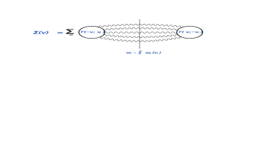
Figure 7: The graphical representation for the formula of Eq. (3.59), for the Pomeron self-energy $\Sigma_{n}$.

Figure 8: The diagrams for the multi-Pomeron vertices. Fig. a) shows the simplest $1\to 2$ vertex. Fig. b) and Fig. c) show the $1\to 3$ vertices, and Figs. d) - i) show the $1\to 4$ vertices. The dashed lines show the cross sections with different energy ($\omega$) propagators. Wavy lines describe the BFKL Pomerons.

The diagrams for the $1\to n$ Pomeron vertices are shown in Fig. 8. The simplest diagram for the $1\to 2$ vertex shown in Fig. 8 a), was calculated in the previous section in detail. It is useful to illustrate the main steps of this calculation, since this approach can be easily generalized to the calculation of the $1\to n$ vertex, for arbitrary $n$. We draw attention to the formula for the $1\to 2$ vertex given in Eq. (2.12). Recall that in this formula, $\nu$ is the scaling dimension of the Parent Pomeron, and $\nu_{1},\nu_{2}$ are the scaling dimensions of the two daughter Pomerons, that are produced at the vertex. The dominant contribution to the $1\to 2$ vertex stems from the singular region $i/2-\nu\,=\,\nu_{1}+\nu_{2}$. Closing the integration contour around this pole, leads to the conservation relation:

$$i/2-\nu\,=\,\nu_{1}+\nu_{2}\hskip 28.45274pt\mbox{or}\hskip 28.45274pt\lambda_{12}\,=\,\lambda_{1}\,+\,\lambda_{2}$$ (3.60)

where $\lambda_{12}\,=\,i/2-\nu$ and $\lambda_{i}\,=\,\nu_{i}\,\,\,(i=1,2)$. The values of $\nu_{1}$ and $\nu_{2}$ are small, since this leads to the dominant $Y$-dependence of the simple loop of Fig. 2, proportional to $\exp\left(2\omega_{0}Y\right)$. Hence from Eq. (3.60) we can conclude that $\nu\to i/2$, (or in other words $i/2-\nu=\lambda_{12}\to 0$) at the $1\to 2$ vertex.

Now we generalize to the notation $\nu_{i}$ $(i=1,2,\dots,n)$, where $\nu_{i}$ denotes the scaling dimension of the $n$ daughter Pomerons, produced from the $1\to n$ vertex. The values of the $\nu_{i}$’s are small, which leads to the $Y$-dependence of the diagrams proportional to $\exp\left(n\omega_{0}Y\right)$. At the simplest $1\to 2$ vertex (see Fig. 8 a) ) where $\nu_{12}\to\nu_{1},\nu_{2}$, the conservation law $i/2-\nu_{12}=\nu_{1}+\nu_{2}$ holds. Hence for $\nu_{1},\nu_{2}$ small, then $\nu_{12}=i/2$. At the $1\to 3$ vertex shown for example in Fig. 8 b) $\nu_{123}\to\nu_{12},\nu_{3}$, and at the $1\to 4$ vertex shown for example in Fig. 8 h), $\nu_{1234}\to\nu_{12},\nu_{34}$.In general this leads to the conservation rule at large $n$:

$$\nu_{12\dots n}=i\left(n-1\right)/2+\sum^{n}_{i=1}\lambda_{i}\hskip 28.45274pt\lambda_{i}\ll 1$$ (3.61)

where the scaling dimensions of the produced Pomerons, are denoted by $\lambda_{i}$, where $\lambda_{i}\ll 1$. Here $n$ is the integer number which counts the number of Pomerons produced in the tree decay, that started with one Pomeron. Within the general $1\to n$ vertex diagram, $\nu_{12\dots n}$ is close to $i\left(n-1\right)/2$. Note that Fig. 8 a) contains one vertex, Fig. 8 b) contains 2 vertices and Fig. 8 d) contains 3 vertices, such that one can generalize to the $1\to n$ vertex that contains $n-1$ sets of $1\to 2$ vertices. The expression for the $1\to 3$ vertex diagrams, as illustrated in Fig. 8 b) and Fig. 8 c) can be written as follows:

$$\Gamma\left(\nu_{123}\,|\,\nu_{1},\nu_{2},\nu_{3}\right)\hskip 8.5359pt=\hskip 8.5359pt$$ (3.62)

$$=\hskip 8.5359pt\left\{\,\,\,\frac{\Gamma\left(\nu_{123}\,|\,\nu_{12},\nu_{3}\right)\,g\left(\nu_{12}\right)\,\Gamma\left(\nu_{12}\,|\,\nu_{1},\nu_{2}\right)}{\omega\,\,-\,\,\omega(\nu_{12})\,\,-\,\,\omega(\nu_{3})}\,\hskip 8.5359pt+\hskip 8.5359pt\frac{\Gamma\left(\nu_{123}\,|\,\nu_{23},\nu_{1}\right)\,g\left(\nu_{23}\right)\,\,\Gamma\left(\nu_{23}\,|\,\nu_{2},\nu_{3}\right)}{\omega\,\,-\,\,\omega(\nu_{23})\,\,-\,\,\omega(\nu_{1})}\right\}_{\omega=\sum^{3}_{i=1}\omega(\nu_{i})}$$

In Eq. (4), $\omega=\sum^{3}_{i=1}\omega\left(\nu_{i}\right)$ because we are taking the residue of the $\omega$-plane pole $1/\left(\omega-\sum^{3}_{i=1}\omega\left(\nu_{i}\right)\right)$, which comes from the cut in the diagrams of Fig. 8 (b) and Fig. 8 (c), that cuts all 3 Pomerons. Eq. (4) can be be written as

$$\Gamma\left(\nu_{123}\,|\,\nu_{1},\nu_{2},\nu_{3}\right)\,\,=\,\,\,\Gamma\left(\nu_{123}\,|\,\nu_{12},\nu_{3}\right)\,\hat{\Gamma}\left(\nu_{12}\,|\,\nu_{1},\nu_{2}\right)\,\,\,+\,\,\Gamma\left(\nu_{123}\,|\,\nu_{23},\nu_{1}\right)\,\hat{\Gamma}\left(\nu_{23}\,|\,\nu_{2},\nu_{3}\right)$$ (3.63)

where the following definition was introduced:

$$\hat{\Gamma}\left(\nu_{12}\,|\,\nu_{1},\nu_{2}\right)\hskip 8.5359pt=\hskip 8.5359pt\frac{g\left(\nu_{12}\right)\Gamma\left(\nu_{12}\,|\,\nu_{1},\nu_{2}\right)}{\omega\left(\nu_{1}\right)+\omega\left(\nu_{2}\right)-\omega\left(\nu_{12}\right)}\,$$ (3.64)

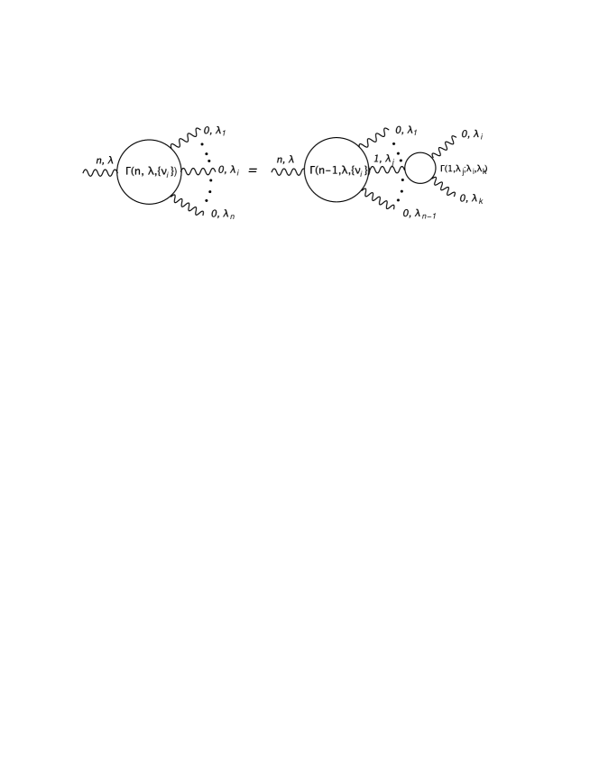
Figure 9: The graphic form of the equation for $\hat{\Gamma}$, given in Eq. (3.65)

with a similar definition for $\hat{\Gamma}\left(\nu_{23}\,|\,\nu_{2},\nu_{3}\right)$. The equation for the vertex where 1 Pomeron $\to\,\,\,n$ Pomerons is shown in Fig. 9. The equation for the vertex takes the following form:

$$\hat{\Gamma}\left(n,\lambda\,|\,\{\lambda_{i}=\nu_{i}\}\right)\,\,\,=\,\,\,\sum^{n-1}_{j=1}\hat{\Gamma}\left(n-1,\lambda\,|\,\{\lambda_{i}\},\lambda_{j}\right)\,\hat{\Gamma}\left(2,\lambda_{j}\,|\,\lambda_{i},\lambda_{k}\right)$$ (3.65)

where

$$\hat{\Gamma}\left(2,\lambda_{ik}\,|\,\lambda_{i},\lambda_{k}\right)\hskip 8.5359pt=\hskip 8.5359ptg\left(\lambda_{ik}\right)\frac{\Gamma\left(\lambda_{ik}\,|\,\lambda_{i},\lambda_{k}\,\right)}{\omega\left(\lambda_{ik}\right)-\omega\left(\lambda_{i}\right)-\omega\left(\lambda_{k}\right)}$$ (3.66)

This equation tells us, that the emission of one extra Pomeron (shown by a zigzag line in Fig. 10), can be reduced to the emission of one extra Pomeron from the produced $(n-1)$ daughter Pomerons. Diagrams where the extra Pomeron is emitted elsewhere in the decay tree, cancel. Indeed, the vertex for one Pomeron emission $\Gamma\left(2,\lambda|\nu_{i},\nu_{k}\right)$ can be re-written in the form

$$\Gamma\left(2,\lambda_{ik}|\lambda_{i},\lambda_{k}\right)\,\,\,=\,\,\hat{\Gamma}\left(2,\lambda_{ik}|\lambda_{i},\lambda_{k}\right)\,\Big{\{}\,\,G^{-1}\left(\omega,\Sigma^{(1)}\right)\,\,-\,\,G^{-1}\left(\omega,\Sigma^{(2)}\right)\,\,\Big{\}}$$ (3.67)

where, using the example of Fig. 10 - B:

$$G^{-1}\left(\omega,\Sigma^{(1)}\right)\hskip 8.5359pt=\hskip 8.5359pt\omega-\Sigma^{(1)}\hskip 8.5359pt=\hskip 8.5359pt\omega-\omega\left(\lambda_{012}\right)-\omega\left(\lambda_{3}\right)$$ (3.68)

$$G^{-1}\left(\omega,\Sigma^{(2)}\right)\hskip 8.5359pt=\hskip 8.5359pt\omega-\Sigma^{(2)}\hskip 8.5359pt=\hskip 8.5359pt\omega-\omega\left(\lambda_{0}\right)-\omega\left(\lambda_{12}\right)-\omega\left(\lambda_{3}\right)$$ (3.69)

Using this Ward identity we can show, that thanks to the cancellations of the diagrams, (as shown by the example of Fig. 10), the emission of the extra Pomeron occurs only from the produced $(n-1)$ daughter Pomerons in the final state. Diagrams where the extra Pomeron is produced from intermediate Pomerons in the decay tree, cancel. In Fig. 10 we show the use of the Ward identity when calculating the $1\to 4$ vertex, in terms of the $1\to 3$ vertex. The blob in Fig. 10 is used to denote the product of two vertices $\hat{\Gamma}(1\to 2)\,\hat{\Gamma}(1\to 2)$ without any $G(\omega,\nu_{ik})$ between them. After summing all of the diagrams in Fig. 10-A,Fig. 10-B and Fig. 10-C, one can see that $\hat{\Gamma}(4,\lambda|\nu_{1},\nu_{2},\nu_{3},\nu_{4})\,\,=\,\,\sum_{i=1}^{3}\hat{\Gamma}\left(3,\lambda|\lambda_{ik},\nu_{l},\nu_{j}\right)\hat{\Gamma}\left(2,\lambda_{ik}|\nu_{i},\nu_{k}\right)$ where $i\neq k\neq l\neq j$.

Figure 10: The illustration of the Ward identity of Eq. (3.67). The extra emitted Pomeron is denoted by the zigzag line.

After this general outline of the calculation using Eq. (3.67), we calculate the example of $\Gamma\left(1\to 4\right)$ in more detail. Each diagram of Fig. 10 can be written as a product of three $\hat{\Gamma}\left(2,\lambda_{ik}|\lambda_{i},\lambda_{k}\right)$ terms. Since $\hat{\Gamma}\left(2,\lambda_{ik}|\lambda_{i},\lambda_{k}\right)\,\propto\lambda_{ik}/(\lambda_{i}\lambda_{k})$ (see Eq. (3.74) below), one can see that this product turns out to be the same for each of the diagrams in Fig.10. Having this in mind, and using Eq. (3.67) we have for the diagram of Fig. 10-B

Fig. 10 - B $$\rightarrow \hat{\Gamma}\left(4,\lambda|\lambda_{0},\lambda_{1},\lambda_{2},\lambda_{3}\right)\,=\,\hat{\Gamma}\left(2,\lambda|\lambda_{012},\lambda_{3}\right)\hat{\Gamma}\left(\lambda_{012}|\lambda_{12},\lambda_{0}\right)\hat{\Gamma}\left(\lambda_{12}|\lambda_{1},\lambda_{2}\right)$$ (3.70)

$$\times G\left(\omega,\Sigma^{(2)}\right)\Big{\{}\,\,G^{-1}\left(\omega,\Sigma^{(1)}\right)\,\,-\,\,G^{-1}\left(\omega,\Sigma^{(2)}\right)\,\,\Big{\}}G\left(\omega,\Sigma^{(1)}\right)\,\,G^{-1}\left(\omega,\Sigma^{(1)}\right)$$

$$= \prod^{3}_{i=1}\hat{\Gamma}_{i}\Big{\{}G\left(\omega,\Sigma^{(2)}\right)\,G^{-1}\left(\omega,\Sigma^{(1)}\right)\,-\,\,1\Big{\}}$$

Here $\prod^{3}_{i=1}\hat{\Gamma}_{i}$ is used to denote the product of corresponding $\hat{\Gamma}$ terms, since it does not depend on the diagram. The first term in Eq. (3.70) describes the emission from the produced Pomerons and has the same structure as the diagram of Fig. 10-A at $\omega=\sum^{3}_{i=0}\omega\left(\lambda_{i}\right)$. Indeed, $\hat{\Gamma}$ for this diagram has the form

Fig. 10 - A $$\rightarrow \hat{\Gamma}\left(4,\lambda|\lambda_{0},\lambda_{1},\lambda_{2},\lambda_{3}\right)\,=\,\hat{\Gamma}\left(2,\lambda|\lambda_{012},\lambda_{3}\right)\hat{\Gamma}\left(\lambda_{012}|\lambda_{02},\lambda_{1}\right)\hat{\Gamma}\left(\lambda_{02}|\lambda_{0},\lambda_{2}\right)$$ (3.71)

$$\times G\left(\omega,\Sigma^{(2)}\right)\,\Big{(}-\omega\left(\lambda_{012}\right)+\omega\left(\lambda_{1}\right)+\omega\left(\lambda_{02}\right)\Big{)}\frac{1}{\omega-\omega\left(\lambda_{012}\right)-\omega\left(\lambda_{3}\right)}G^{-1}\left(\omega,\Sigma^{(1)}\right)$$

$$\xrightarrow{\omega=\sum^{3}_{i=0}\omega\left(\lambda_{i}\right)} \prod^{3}_{i=1}\hat{\Gamma}_{i}G\left(\omega,\Sigma^{(2)}\right)\,G^{-1}\left(\omega,\Sigma^{(1)}\right)$$

The difference between Eq. (3.71) and the first term in Eq. (3.70) is in the expression for $\Sigma^{(2)}$ which is equal to $\Sigma^{(2)}\,=\,\omega\left(\lambda_{1}\right)+\omega\left(\lambda_{02}\right)+\omega\left(\lambda_{3}\right)$ instead of Eq. (3.69).

The second term in Eq. (3.70) cancels with the diagram of Fig. 10-C. This diagram is actually equal to sum of the two terms shown in Fig. 8-h and Fig. 8-i. This sum is equal to the following expression.

Fig. 10 - c $$\rightarrow \hat{\Gamma}\left(4,\lambda|\lambda_{0},\lambda_{1},\lambda_{2},\lambda_{3}\right)\,=\prod^{3}_{i=1}\hat{\Gamma}_{i}\frac{1}{\omega\,-\,\omega\left(\lambda_{12}\right)-\omega\left(\lambda_{03}\right)}$$ (3.72)

$$\times \left\{\left(\omega\left(\lambda_{0}\right)+\omega\left(\lambda_{3}\right)-\omega\left(\lambda_{03}\right)\right)\frac{\omega\left(\lambda_{0}\right)+\omega\left(\lambda_{3}\right)-\omega\left(\lambda_{03}\right)}{\omega-\omega\left(\lambda_{03}\right)-\omega\left(\lambda_{1}\right)-\omega\left(\lambda_{2}\right)}\right.\,$$

$$+ \,\left.\left(\omega\left(\lambda_{1}\right)+\omega\left(\lambda_{2}\right)-\omega\left(\lambda_{12}\right)\right)\frac{\omega\left(\lambda_{1}\right)+\omega\left(\lambda_{2}\right)-\omega\left(\lambda_{12}\right)}{\omega-\omega\left(\lambda_{12}\right)-\omega\left(\lambda_{0}\right)-\omega\left(\lambda_{3}\right)}\right\}$$

$$\xrightarrow{\omega=\sum^{3}_{i=0}\omega\left(\lambda_{i}\right)} \,\,\,\,\prod^{3}_{i=1}\hat{\Gamma}_{i}$$

Summarizing we see that Eq. (3.67) leads to the cancellation of the emission of the Pomeron from the internal lines in the diagram. Such cancellations are analogous to the cancellation in gauge theories since Eq. (3.67) is similar to the Ward identity in these theories.

As discussed above, at the $1\to 2$ vertex, the conservation rule $i/2-\nu_{j}=\nu_{i}+\nu_{k}\,\,(\lambda_{ik}=\lambda_{i}+\lambda_{k})$ (see Eq. (3.60) and the surrounding discussion). We are interested in the region where $\nu_{i}$ and $\nu_{k}$ are small, since this leads to the $Y$-dependence of the diagrams proportional to $\exp\left(n\omega_{0}Y\right)$, which is the dominant contribution. Thus the relevant region is $i/2-\nu_{j}\to 0$. Substituting for $\Gamma\left(\nu_{j}\,|\,\nu_{i},\nu_{k}\,\right)$ the formula of Eq. (2.12), then Eq. (3.66) becomes:

$$\hat{\Gamma}\left(2,\nu_{j}\,|\,\nu_{i},\nu_{k}\right)\hskip 8.5359pt=\hskip 8.5359pt\frac{16\bar{\alpha}_{s}^{2}}{N_{c}}\,\,\,\,g\left(\nu_{j}\right)\,\,\,\,\frac{\left(\Gamma_{\footnotesize{\mbox{planar}}}\left(\nu_{j}\,|\,\nu_{i},\nu_{k}\,\right)-{\frac{2\pi}{N_{c}^{2}}}\Gamma_{\footnotesize{\mbox{nonplanar}}}\left(\nu_{j}\,|\,\nu_{i},\nu_{k}\,\right)\right)}{\omega(\nu_{j})\,-\,\omega(\nu_{i})\,-\,\omega(\nu_{k})}$$ (3.73)

Now to calculate the residue of $\hat{\Gamma}\left(2,\nu_{j}\,|\,\nu_{i},\nu_{k}\right)$ in our region of interest, namely $i/2-\nu_{j}-\nu_{i}-\nu_{k}\to 0$ when $\nu_{i},\nu_{k}\to 0$, simply substitute into Eq. (3.73) the asymptotic formulae for $\Gamma_{\footnotesize{\mbox{planar}}}$ and $\Gamma_{\footnotesize{\mbox{nonplanar}}}$ derived in Eqs. (A.22) and (A.26). Note that in this region, as $i/2-\nu_{j}\to\nu_{i}+\nu_{k}\to 0$ the denominator of Eq. (3.73) tends to $\omega(\nu_{j})\,-\,\omega(\nu_{i})\,-\,\omega(\nu_{k})\to\bar{\alpha}_{s}/\left(\frac{1}{2}+i\nu_{j}\right)$ (see definition of Eq. (A.1) ) and $g\left(\nu_{j}\right)\to-\left(\frac{1}{2}+i\nu_{j}\right)^{-2}/4$ (see definition Eq. (2.8)). With this in mind, overall Eq. (3.73) in this region reads:

$$\lim_{\begin{subarray}{c}i/2-\nu_{j}-\nu_{i}-\nu_{k}\to 0\\ \nu_{i},\nu_{k}\to 0\end{subarray}}\hskip 8.5359pt\hat{\Gamma}\left(2,\nu_{j}\,|\,\nu_{i},\nu_{k}\right)\hskip 8.5359pt=\hskip 8.5359pt\lim_{\begin{subarray}{c}i/2-\nu_{j}-\nu_{i}-\nu_{k}\to 0\\ \nu_{i},\nu_{k}\to 0\end{subarray}}\,b\,\frac{\left(\frac{1}{2}+i\nu_{j}\right)}{\nu_{i}\nu_{k}}$$

$$=\hskip 8.5359pt\lim_{\nu_{i},\nu_{k}\to 0}\hskip 8.5359ptb\,\frac{\,\left(\nu_{i}+\nu_{k}\right)}{\nu_{i}\nu_{k}}\$$ (3.74)

$$b\hskip 8.5359pt=\hskip 8.5359pt\frac{-a}{4\bar{\alpha}_{s}}$$ (3.75)

where the constant $a$ is defined in Eq. (A.28). Now Eq. (3.65) is the equation for the BFKL Pomeron fan diagram. Fan diagrams can be summed using the generating functional technique that has been developed in $\left(Y,\zeta\right)$ representation (see ref. [32] for details). For the generating functional, we can write the linear equation in terms of functional derivatives, which reflects the fact that the Pomeron can decay into two Pomerons. In the dipole model, this decay can be written as the decay of one dipole to two dipoles. Eq. (3.65) simplifies this functional equation to a recursive formula. Two simplification rules are essential for our approach: (i) the most singular part of the triple Pomeron vertex has a much simpler form in $\nu$ representation, than the BFKL kernel in coordinate representation, and (ii) the loop correction to the vertex can be neglected at high energies (see ref. [20] for a full explanation). Eq. (3.65) can be viewed as an equation in time (rapidity). Indeed, Eq. (3.65) states that the process of $n$-Pomeron production can be considered to be the production of $n-1$ Pomerons at time $t$, and the later decay of one of the produced Pomerons into two, at time $t+\delta t$ ($\delta t\ll 1$), as shown in Fig. 9. Using Eq. (3.74) we can rewrite Eq. (3.65) in the following form:

$$\hat{\Gamma}\left(n,\lambda\,|\,\{\nu_{i}\}\right)\hskip 8.5359pt=\hskip 8.5359ptb\,\sum^{n-1}_{j=1}\hat{\Gamma}\left(n-1,\lambda\,|\,\{\nu_{i}\},\nu_{j}\right)\,\left(\,\frac{\nu_{i}+\nu_{k}}{\nu_{i}\,\nu_{k}}\,\right)$$ (3.76)

$$i\neq j\neq k\neq l$$

where on the LHS of Eq. (3.76) the notation $\{\nu_{i}\}=\nu_{1},\nu_{2},\dots\nu_{n}$, whereas on the RHS the notation $\{\nu_{i}\}=\nu_{1},\nu_{2},\dots\nu_{n};\,\,\,\nu_{i}\neq\nu_{j}$. In this approach Eq. (3.76) yields the following solution:

$$\hat{\Gamma}\left(n,\lambda\,|\,\{\nu_{i}\}\right)\,\,\,=\,\,\,\,\lambda\,\left(n-1\right)!\,\prod^{n}_{i=1}\,\Phi\left(\nu_{i}\right)\,\,\,\,\,\mbox{with}\,\,\,\,\,\,\Phi\left(\nu_{i}\right)\,\,=\,\frac{b}{\nu_{i}}$$ (3.77)

It is easy to check that this solution satisfies both the recursive equation (see Eq. (3.76)) and the initial condition of Eq. (3.74).

3.2 Green function of the resulting BFKL Pomeron

Using the formula of Eq. (3.77) for the vertices, we can calculate $\Sigma_{n}\left(\omega,\nu\right)$ from Eq. (3.59) as:

$$\Sigma_{n}\left(\omega,\nu\,=\,i(n-1)/2+\lambda\right)\,\,\,\,=\,\,\,\bar{\alpha}_{s}^{2}\,\left(-1\right)^{n}b^{2n}\frac{(n-1)!}{n}\,\frac{1}{g(\nu)}\,{{\int}}\,\prod_{i}^{n}\frac{d\nu_{i}}{2\pi i}\,\delta\left(\lambda\,-\,\sum^{n}_{i}\nu_{i}\right)\,\frac{1}{\omega\,-\,\sum^{n}_{i}\omega_{i}(\nu_{i})}\hskip 28.45274pt$$ (3.78)

The explanation behind the factor in front in Eq. (3.78), is as follows. The vertices that enter into Eq. (3.78), are equal to $\hat{\Gamma}$ after multiplying by a factor of $\left(\omega\left(\nu\right)-\omega\left(\nu_{1}\right)-\omega\left(\nu_{2}\right)\right)/g(\nu)$ (see the definition of Eq. (3.66)). In the region where $\lambda=i/2-\nu\to 0$, this factor reduces to the asymptote $\bar{\alpha}_{s}/\left(\lambda\,g(\nu)\right)$ for large $n$. The factor of $(-1)^{n}(n-1)!/n$ that appears in Eq. (3.78) has the following meaning:

$$(-1)^{n}(n-1)!/n\,\, = \,\,(-1)^{n-1}\,\mbox{\{ $(-1)$ for each Pomeron loop\}}\,\times\,(n-1)!^{2}\,\mbox{\{ from {Eq.~{}(\ref{SOL1})} \}}$$ (3.79)

$$\times \,\,\frac{1}{n!}\,\mbox{\{ from the identity of the Pomerons\}}\,\times(-1)\,\mbox{\{ from definition of $\Sigma$\}}$$

We do not need to integrate over the entire phase space in $\nu_{i}$, due to the identity of Pomerons. It is enough to integrate within the region $\nu_{n}\,>\,\nu_{n-1}\,>\,\dots\,>\,\nu_{i}\,\dots\,>\nu_{1}$. As one can see, in this region all of the Pomerons have different $\nu$’s, and can be considered to be different particles. This region covers the $1/n!$ part of the entire phase space in $\nu$. Further summation turns out to be simpler in $Y$ and $\ln\zeta=\ln xx^{*}$ representation, where $Y$ is the rapidity of the dipole-dipole scattering, while

$$\zeta\hskip 8.5359pt=\hskip 8.5359ptxx^{*}\hskip 8.5359pt=\hskip 8.5359pt\frac{r^{2}R^{2}}{\left(\vec{b}+\frac{1}{2}(\vec{r}-\vec{R})\right)^{2}\,\left(\vec{b}-\frac{1}{2}(\vec{r}-\vec{R})\right)^{2}}$$ (3.80)

where $\vec{b}$ is the impact parameter of the dipole-dipole scattering, and $\vec{r}$ and $\vec{R}$ are the sizes of the two dipoles. Using these variables, $\Sigma_{n}\left(Y,\zeta\right)$ can be calculated using the following transform:

$$\Sigma_{n}\left(Y,\zeta\right)\,\,=\,\,{{\int}}^{a+i\infty}_{a-i\infty}\frac{d\omega}{2\pi i}\,e^{\omega Y}\,{{\int}}^{ia^{\,\prime}+\infty}_{ia^{\,\prime}-\infty}\frac{d\nu}{2\pi}\,e^{i\nu\ln\zeta}\,\,\Sigma_{n}\left(\omega,\nu\right)$$ (3.81)

First we switch to $Y$ representation using the following inverse Mellin transform:

$$\Sigma_{n}\left(Y,\nu\right)\,\, = \,\,{{\int}}^{a+i\infty}_{a-i\infty}\frac{d\omega}{2\pi i}e^{\omega Y}\Sigma_{n}\left(\omega,\nu\right)\,\,=\,\,\bar{\alpha}_{s}^{2}\,(-1)^{n}\,b^{2n}\frac{(n-1)!}{n}\,\frac{1}{g(\nu)}\,{{\int}}\prod_{i}^{n}\frac{d\nu_{i}}{2\pi i}\,e^{\omega(\nu_{i})\,Y}\,\delta\left(\lambda\,-\,\sum^{n}_{i}\nu_{i}\right)\hskip 28.45274pt$$ (3.82)

Then we switch to $\zeta$ representation using the following approach:

$$\Sigma_{n}\left(Y,\zeta\right)\hskip 8.5359pt=\hskip 8.5359pt{{\int}}^{ia^{\,\prime}+\infty}_{ia^{\,\prime}-\infty}\frac{d\nu}{2\pi}\,e^{i\nu\ln\zeta}\,\,\Sigma_{n}\left(Y,\nu\right)$$

$$=\hskip 8.5359pt\bar{\alpha}_{s}^{2}\,(-1)^{n}b^{2n}\,\frac{(n-1)!}{n}\,\frac{1}{g(\nu)}{{\int}}^{ia^{\,\prime}+\infty}_{ia^{\,\prime}-\infty}\frac{d\nu}{2\pi}\,e^{i\nu\ln\zeta}{{\int}}\prod_{i}^{n}\frac{d\nu_{i}}{2\pi i}\,e^{\omega(\nu_{i})\,Y}\,\delta\left(\lambda\,-\,\sum^{n}_{i}\nu_{i}\right)$$ (3.83)

As we have discussed generally speaking $\nu\,=\,\nu_{n}\,-\,\lambda$. However, the value of $\nu_{n}$ turns out to be different from $(n-1)!$ in general, for various different $1\to n$ vertex diagrams. In Table 1 we give the examples for $1\to n$ vertex diagrams, up to $n=6$.

$\nu_{n}{\Big{/}}\Gamma$	$1\to 2$	$1\to 3$	$1\to 4$	$1\to 5$	$1\to 6$
i	0	0	0	4	0
i/2	1	0	4	0	80
0	0	2	0	16	0
-i/2	0	0	2	4	40

Table 1: The number diagram for the values of $\nu_{n}$ for diffrent vetices $\Gamma$.

Unfortunately, we have not derived the general rules for how to calculate the value of $\nu_{n}$ for the $1\to n$ vertex. We consider two models for such numbers: (i) each $1\to n$ vertex has $\nu_{n}=0$, and (ii) each $1\to n$ vertex has $\nu_{n}=i(n-1)/2$. The first model gives the sum of the leading twist contribution $\zeta^{i\nu}\to 1$, while the second model sums over all high twists $\zeta^{i\nu}\to\zeta^{-n/2}$. We believe that considering these two models for finding the value of $\nu_{n}$, provides the largest possible contributions. This belief is based on the following simple examples. As can be seen from Eq. (3.83), we are summing an asymptotic series of the form:

$$\sum^{\infty}_{n=0}(-1)^{n}\,C_{n}\,L^{n}$$ (3.84)

where $L$ is a large parameter. Our first model means that for the leading twist contribution, we choose $\nu_{n}=0$ in all $n!$-diagrams. This leads to $C_{n}\propto n!$. In the exact approach, the number of diagrams with $\nu_{n}=0$ is less than $n!$. However, the largest sum corresponds to $C_{n}=n!$. One can see this by setting $C_{n}=1$ and $C_{n}=1/n!$ in Eq. (3.84). The same occurs in the second model, which we believe leads to the maximal sum of the highest twist contributions.

3.3 Summing high twists

Recall that $\nu\hskip 8.5359pt=\hskip 8.5359pti(n-1)/2+\lambda\approx i(n-1)/2$ at large $n$, such that after switching to the integration variable $\lambda$, then Eq. (3.83) can be written as:

$$\Sigma_{n}\left(Y,\zeta\right)\,\,=\,\,\zeta^{(1-n)/2}\,\frac{\bar{\alpha}_{s}^{2}}{4}\,(n-1)^{2}\,b^{2n}\,(-1)^{n-1}\,\frac{(n-1)!}{n}\,{{\int}}^{ia^{\,\prime}+\infty}_{ia^{\,\prime}-\infty}\frac{d\lambda}{2\pi}\,e^{i\lambda\ln\zeta}\,{{\int}}\prod_{i=1}^{n}\frac{d\nu_{i}}{2\pi i}\,e^{\omega(\nu_{i})\,Y}\,\delta\left(\lambda\,-\,\sum^{n}_{i}\nu_{i}\right)$$

$$=\,\,\zeta^{(1-n)/2}\,\frac{\bar{\alpha}_{s}^{2}}{4}\,(n-1)^{2}\,b^{2n}\,(-1)^{n-1}\,\frac{(n-1)!}{n}\,{{\int}}\prod^{n}_{i=1}\frac{d\nu_{i}}{2\pi i}\,\,\,e^{\omega(\nu_{i})\,Y+i\,\nu_{i}\ln\zeta}$$ (3.85)

where we took the integral over $\lambda$ using the $\delta$-function. Using Eq. (A.4) we can solve the integral over $\nu_{i}$ explicitly, using the method of steepest descents. In this approach Eq. (3.85) simplifies to:

$$\Sigma_{n}\left(Y,\zeta\right)\hskip 8.5359pt=\hskip 8.5359pt\zeta^{(1-n)/2}\,\frac{\bar{\alpha}_{s}^{2}}{4}\,\,b^{2n}\,(-1)^{n-1}\,\frac{(n-1)^{2}}{n}(n-1)!\,\,\left(\sqrt{\frac{\pi}{DY}}\,e^{\omega(0)Y-\ln^{2}\zeta/(4DY)}\right)^{n}$$ (3.87)

$$=\hskip 8.5359pt\frac{\bar{\alpha}_{s}^{2}}{4}\,\sqrt{\zeta}\,\,\,(-1)^{n-1}\,\frac{(n-1)^{2}}{n}\,\Gamma\left(n\right)\,L^{n}\,$$

where $$L\hskip 8.5359pt=\hskip 8.5359ptb^{2}\,\,\sqrt{\frac{\pi\,}{D\,Y\zeta}}\,\exp\left(\omega(0)\,Y\,\,-\,\,\frac{\ln^{2}\zeta}{4\,D\,Y}\right)$$ (3.88)

Using the integral representation for the Euler-Gamma function (see formula 8.310(1) of ref. [33]):

$$\Gamma\left(n+1\right)\,=\,\int^{\infty}_{0}\,t^{n}\,e^{-\,t}\,dt;$$ (3.89)

and since we are summing from $n=2$, (since the first $1\to n$ vertex in the sum is the $1\to 2$ vertex), we obtain the following result for $\Sigma\left(Y,\zeta\right)$:

$$\Sigma\left(Y,\zeta\right)\hskip 8.5359pt=\hskip 8.5359pt\,\sum_{n=2}^{\infty}\,\Sigma_{n}\left(Y,\zeta\right)\hskip 8.5359pt=\hskip 8.5359pt-\frac{\bar{\alpha}_{s}^{2}}{4}\,\sqrt{\zeta}\,{{\int}}^{\infty}_{0}e^{-t}\,\frac{dt}{t}\,\sum^{\infty}_{n=2}\,\,\frac{(n-1)^{2}}{n}\left(-tL\right)^{n}$$

$$=\hskip 8.5359pt\,\,-\,\frac{\bar{\alpha}_{s}^{2}}{4}\,\,\sqrt{\zeta}\,{{\int}}^{\infty}_{0}\,\frac{dt}{t}\,e^{-t}\,\left\{\frac{Lt+2(Lt)^{2}-\ln(1+Lt)-2Lt\ln(1+Lt)-(Lt)^{2}\ln(1+Lt)}{(1+Lt)^{2}}\,\right\}$$

$$=\hskip 8.5359pt\,\,-\,\frac{\bar{\alpha}_{s}^{2}}{4}\,\,\sqrt{\zeta}\,\,{{\int}}^{\infty}_{0}\,\frac{dT}{T}\,e^{-T/L}\,\frac{T+2T^{2}-\ln(1+T)-2T\ln(1+T)-T^{2}\ln(1+T)}{(1+T)^{2}}$$

$$=\hskip 8.5359pt\,\,\,\frac{\bar{\alpha}_{s}^{2}}{4}\,\,\sqrt{\zeta}\,\Sigma\left(L\right)$$ (3.90)

where $T=Lt$. For large $L$ we find that

$$\Sigma\left(L\right)\,\, \xrightarrow{L\gg 1} \,{{\int}}^{\infty}_{0}\,\frac{dT}{T}e^{-T/L}\left(2-\ln T+\mathcal{O}\left(\frac{\ln T}{T}\right)\right)\,\,\,\approx\,\,\,{{\int}}^{L}_{0}\,\frac{dT}{T}\left(-\ln T\right)\,\,=\,\,-\,(\ln L)^{2}/2$$ (3.91)

Inserting Eq. (3.91) into Eq. (3.3), using the definition for $L$ given in Eq. (3.88), we see that at large $Y$ and in terms of $\ln\zeta$, then $\Sigma\left(Y,\zeta\right)$ tends to the following simple formula:

$$\Sigma\left(Y,\zeta\right)\,\,\,=\,\,\,\frac{\bar{\alpha}_{s}^{2}}{8}\,\,\sqrt{\zeta}\,\left(\,\omega_{0}Y\,-\,\frac{\ln^{2}\zeta}{4DY}\,-\,\frac{1}{2}\ln Y\,-\frac{1}{2}\ln\zeta\,+\,\ln\left(b^{2}\sqrt{\frac{\pi}{D}}\right)\right)^{2}$$ (3.92)

Using the following formula to transform to $\left(\,\omega,\nu\,\right)$ representation:

$$\Sigma\left(\omega,\nu\right)\hskip 8.5359pt=\hskip 8.5359pt{{\int}}^{\infty}_{0}d\zeta\,\zeta^{\,-1-i\nu}{{\int}}^{\infty}_{0}dY\,e^{-\omega Y}\Sigma\left(Y,\zeta\right)\hskip 8.5359pt=\hskip 8.5359pt{{\int}}^{\infty}_{-\infty}d\ln\zeta\,e^{\,-i\nu\,\ln\zeta}{{\int}}^{\infty}_{0}dY\,e^{-\omega Y}\Sigma\left(Y,\zeta\right)$$ (3.93)

Note that Eq. (3.93) is the double Mellin transform from $\left(Y,\zeta\right)$ to $\left(\omega,\nu\right)$ representation. This corresponds to the inverse-Mellin transform of Eq. (3.81) which was used to transform from $\left(\omega,\nu\right)$ to $\left(Y,\zeta\right)$ representation. Then inserting Eq. (3.92) into Eq. (3.93) for large $Y$, leads to the following equation for $\Sigma\left(\omega,\nu\right)$:

$$\Sigma\left(\omega,\nu\right)\,\,\xrightarrow{\omega\to 0}\,\,\frac{\bar{\alpha}_{s}^{2}}{8}\,\,\frac{1}{\left(i\nu\,+\,{\frac{1}{2}}\right)}\,\frac{\left(2\,\omega^{2}_{0}\,\,+\,\,\omega_{0}\,\omega\,\ln\omega\,\,+\,\,\,\mathcal{O}\left(\omega^{2}\right)\,\right)}{\omega^{3}}$$ (3.94)

where the last term $\mathcal{O}\left(\omega^{2}\right)$, labels small terms proportional to $\omega^{2}$. In reality, due to the $\omega^{3}$ term in the denominator of Eq. (3.94), then overall this $\mathcal{O}\left(\omega^{2}\right)$ term, leads to terms which are singular in powers of just $1/\omega$, and hence smaller than the singular terms by powers of $1/\omega^{2}$ and $1/\omega^{3}$ that come before. The Green function of the dressed Pomeron reads:

$$G\left(\omega,\nu\right)\,\,=\,\,\frac{1}{\omega-\omega\left(\nu\right)+\Sigma\left(\omega,\nu\right)}\,\,=\,\,\frac{1}{\omega-\omega\left(\nu\right)\,+\,{\frac{\bar{\alpha}_{s}^{2}}{8}\,\,\frac{1}{\left(i\nu+{\frac{1}{2}}\right)}\,\left(\frac{2\,\omega^{2}_{0}}{\omega^{3}}\,\,+\,\,\,\omega_{0}\,\frac{\ln\omega}{\omega^{2}}\right)}}$$ (3.95)

For small $\omega$ and $\nu$, we can neglect the contribution from $G_{0}^{-1}\left(\omega,\nu\right)=\omega-\omega\left(\nu\right)$. Therefore, in this limit the Green function of the dressed Pomeron is given by the following formula:

$$G\left(\omega,\nu\right) \,\,\xrightarrow{\omega\to 0}\,\,\frac{{\frac{8}{\bar{\alpha}_{s}^{2}}\,\frac{\omega^{3}}{\omega_{0}}}\,\left({\frac{1}{2}}+i\nu\right)}{\left(\,2\,\omega_{0}+\,\,\omega\,\ln\omega\,\right)}$$ (3.97)

$$\,\,\xrightarrow{\omega\to 0}\,\,\frac{4}{\bar{\alpha}_{s}^{2}}\frac{\omega^{3}}{\omega^{2}_{0}}\,\,\left(i\nu+\frac{1}{2}\right)$$

where in Eq. (3.97) the second term in the denominator of Eq. (3.97) is neglected in the limit that $\omega\to 0$. One can see that Eq. (3.97) leads to the function that has no singularity at $\omega\to 0$ and therefore, the corresponding imaginary part of the scattering amplitude vanishes. To gain a better understanding, keeping the second term in the denominator of Eq. (3.97) yields:

$$G\left(\omega,\nu\right)\,\,=\,\frac{4}{\bar{\alpha}_{s}^{2}}\frac{\omega^{3}}{\omega_{0}^{2}}\,\,\left(\frac{1}{2}+i\nu\right)\,\left(1\,\,-\,\,\frac{\omega\,\ln\omega}{2\omega_{0}}\right)\,\,=\,\,G^{(1)}\left(\omega,\nu\right)\,\,+\,\,G^{(2)}\left(\omega,\nu\right)$$ (3.98)

Passing to ($Y,\zeta$)-representation we see that the asymptotic behaviour of the Pomeron Green function is

$$G\left(Y,\zeta\right)\hskip 8.5359pt =\hskip 8.5359pt{{\int}}^{ia^{\,\prime}+\infty}_{ia^{\,\prime}-\infty}\frac{d\nu}{2\pi}\,e^{\,i\nu\ln\zeta}{{\int}}^{a+i\infty}_{a-i\infty}\frac{d\omega}{2\pi i}\,e^{\,\omega Y}\,G\left(\omega,\nu\right)\,$$ (3.99)

$$=\hskip 8.5359pt\,{{\int}}^{ia^{\,\prime}+\infty}_{ia^{\,\prime}-\infty}\frac{d\nu}{2\pi}\,e^{\,i\nu\ln\zeta}{{\int}}^{a+i\infty}_{a-i\infty}\frac{d\omega}{2\pi i}\,e^{\,\omega Y}\,G^{(2)}\left(\omega,\nu\right)$$

$$=\hskip 8.5359pt-\,\frac{2}{\bar{\alpha}_{s}^{2}\,\omega^{3}_{0}}\,\,\left({\frac{1}{2}}+\frac{\partial}{\partial\ln\zeta}\right)\,\delta\left(\ln\zeta\right){{\int}}^{\infty}_{0}\,d\omega\,e^{\,\,\omega Y}\,\,\omega^{4}\ln\omega$$

Closing the contour of integration on the real negative $\omega$-axis, we have:

$$G\left(Y,\zeta\right)\hskip 8.5359pt =\hskip 8.5359pt\,\,\frac{2}{\bar{\alpha}_{s}^{2}\,\omega^{3}_{0}}\,\,\left({\frac{1}{2}}+\frac{\partial}{\partial\ln\zeta}\right)\,\delta\left(\ln\zeta\right){{\int}}^{\infty}_{0}\,d\omega\,e^{\,-\,\omega Y}\,\,\omega^{4}\,$$ (3.100)

$$=\hskip 8.5359pt\,\,\,\,\,\,\frac{2}{\bar{\alpha}_{s}^{2}\,\omega^{2}_{0}}\,\,\left({\frac{1}{2}}+\frac{\partial}{\partial\ln\zeta}\right)\,\delta\left(\ln\zeta\right)\,\frac{4!}{Y^{5}}$$

From Eq. (3.100) its clear that the Green function leads to the cross section that decreases as $1/Y^{5}$, and the character of this asymptotic behaviour depends on $\zeta$. The factor that depends on $\zeta$, in front of Eq. (3.100), indicates that the main contribution turns out to be a leading twist contribution.

This decrease at ultra high energies is the most salient result of this paper. It is well known that the Pomeron calculus in zero transverse dimensions, leads to the Green function of the Pomeron that decreases with energy, (see refs. [21, 22, 23, 24, 25]). However, in our case the decrease of the cross section is only logarithmic, whereas in the Pomeron calculus in zero transverse dimensions, the cross section falls exponentially at large $Y$. Therefore, we claim that the BFKL evolution of the sizes of the interacting dipoles, do not lead to a new qualitative effect. However, it is interesting that the character of the asymptotic behaviour, crucially depends on the size of the interacting dipole.

3.4 Summing the leading twist contribution

In the previous subsection we demonstrated that summing the contribution of high twists, leads to the solution which appears to be the leading twist contribution. Therefore, it seems reasonably possible to derive the leading twist contribution. We will do this assuming that $\nu_{n}=0$ for every odd $n$ (see Table I). Recalling that $g(\nu)\to 16\nu^{2}$ as $\nu\to 0$, and using the formula $\nu=\nu_{n}-\lambda$ then we can re-write Eq. (3.83) in the form

$$\Sigma_{n}\left(Y,\zeta\right)\hskip 8.5359pt=\hskip 8.5359pt{{\int}}^{ia^{\,\prime}+\infty}_{ia^{\,\prime}-\infty}\frac{d\lambda}{2\pi}\,e^{i\lambda\ln\zeta}\,\,\Sigma_{n}\left(Y,\lambda\right)$$

$$=\hskip 8.5359pt\bar{\alpha}_{s}^{2}\,(-1)^{n}b^{2n}\,\frac{(n-1)!}{n}\ {{\int}}^{ia^{\,\prime}+\infty}_{ia^{\,\prime}-\infty}\frac{d\lambda}{2\pi}\,\frac{1}{16\,\lambda^{2}}\,e^{i\lambda\ln\zeta}{{\int}}\prod_{i}^{n}\frac{d\nu_{i}}{2\pi i}\,e^{\omega(\nu_{i})\,Y}\,\delta\left(\lambda\,-\,\sum^{n}_{i}\nu_{i}\right)$$ (3.101)

Using the following representation for the $\delta$- function, namely,

$$\delta\left(\lambda\,-\,\sum^{n}_{i=1}\nu_{i}\right)\,\,=\,\,\frac{1}{2\pi}{{\int}}^{\infty}_{-\infty}\,d\mu\,e^{i\mu\,\left(\lambda\,-\,\sum^{n}_{i=1}\nu_{i}\right)}$$ (3.102)

and integrating over $\lambda$ by closing the integration contour around the double pole at $\lambda=0$, we obtain

$$\Sigma_{n}\left(Y,\zeta\right)\hskip 8.5359pt=\hskip 8.5359pt\frac{\bar{\alpha}_{s}^{2}}{16}\,(-1)^{n}\,b^{2n}\,\frac{(n-1)!}{n}\,\,\frac{1}{2\pi}{{\int}}^{\infty}_{-\infty}\,d\mu\,\left(i\ln\zeta+i\mu\right)\prod^{n}_{i=1}{{\int}}\frac{d\nu_{i}}{2\pi i}\,e^{-i\nu_{i}\,\mu\,\,+\,\,\omega(\nu_{i})\,Y}$$

Integrating over $\nu_{i}$ using the method of steepest descents, we have:

$$\Sigma_{n}\left(Y,\zeta\right)\hskip 8.5359pt=\hskip 8.5359pt\frac{\bar{\alpha}_{s}^{2}}{16}\,(-1)^{n}b^{2n}\,\frac{(n-1)!}{n}\,\,\frac{1}{2\pi}{{\int}}^{\infty}_{-\infty}\,d\mu\,\left(i\ln\zeta+i\mu\right)\left(\sqrt{\frac{\pi}{D\,Y}}\,\exp\left(\omega_{0}Y\,\,-\,\,{\frac{\mu^{2}}{4DY}}\right)\right)^{n}$$ (3.104)

Finally after solving the $\mu$ integral, using the result that ${{\int}}^{\infty}_{-\infty}dx\exp\left(-ax^{2}\right)\hskip 8.5359pt=\hskip 8.5359pt\sqrt{\pi/a}$ yields:

$$\Sigma_{n}\left(Y,\zeta\right)\hskip 8.5359pt=\hskip 8.5359pt\frac{\bar{\alpha}_{s}^{2}}{16}\,\ln\zeta\,(-1)^{n}\,\,\frac{(n-1)!}{n}\sqrt{\frac{D\,Y}{\pi\,n}}\,L^{n}$$ (3.105)

$$L\hskip 8.5359pt=\hskip 8.5359ptb^{2}\,\,\sqrt{\frac{\pi\,}{D\,Y}}\,e^{\omega(0)\,Y}$$ (3.106)

Using Eq. (3.89) we can re-write Eq. (3.106) in the form

$$\Sigma\left(Y,\zeta\right) \hskip 8.5359pt=\hskip 8.5359pt \frac{\bar{\alpha}_{s}^{2}}{16}\,\sqrt{\frac{D\,Y}{\pi}}\,\ln\zeta\,\sum^{\infty}_{n=2}\,(-1)^{n}\,\,\frac{(n-1)!}{n^{3/2}}\,\,L^{n}\,$$ (3.107)

$$= \,\,\frac{\bar{\alpha}_{s}^{2}}{16}\,\sqrt{\frac{D\,Y}{\pi}}\,\ln\zeta\,{{\int}}^{\infty}_{0}dt\,e^{-t}\sum^{\infty}_{n=2}\,(-1)^{n}\,\,\frac{L^{n}t^{n-1}}{n^{3/2}}\,\,$$

$$= \frac{\bar{\alpha}_{s}^{2}}{16}\,\sqrt{\frac{D\,Y}{\pi}}\,\ln\zeta\,{{\int}}^{\infty}_{0}\frac{dt}{t}\,e^{-t}\,\Big{(}Lt\,\,+\,\,Li_{3/2}\left(-Lt\right)\Big{)}$$

For properties of the Polylogarithm function see Ref.[36]. Since we assumed that $\nu_{n}=0$ occurs only at odd $n$, we can extract this from the sum of Eq. (3.107), by subtracting from it the function where $L\to-L$. In this approach, finally we arrive at the expression:

$$\Sigma\left(Y,\zeta\right)\hskip 8.5359pt=\hskip 8.5359pt\frac{\bar{\alpha}_{s}^{2}}{16}\,\sqrt{\frac{D\,Y}{\pi}}\,\ln\zeta\,\left(\,2L\,+\,{{\int}}^{\infty}_{0}\frac{dT}{T}\,\exp\left(-T/L\right)\,\left(\,Li_{3/2}\left(-T\right)\,\,-\,\,\,Li_{3/2}\left(T\right)\right)\,\right)\,\,$$ (3.108)

$$=\,\,\frac{\bar{\alpha}_{s}^{2}}{16}\,\sqrt{\frac{D\,Y}{\pi}}\,\ln\zeta\,\Sigma\left(L\right)$$ (3.109)

where $T=Lt$. Since the asymptotic behaviour of the Polylogarithm function $Li_{s}(-T)$ is known, namely

$$Li_{s}\left(-T\right)\,\,\xrightarrow{T\gg 1}\,\,-\frac{\ln^{s}\left(T\right)}{\Gamma(1+s)}\,$$ (3.110)

Then with this in mind, the integral of Eq. (3.108) is expected to lead to the following result:

$$\Sigma\left(L\right)\hskip 8.5359pt=\hskip 8.5359pt2L+{{\int}}^{\infty}_{0}\frac{dT}{T}\,\exp\left(-T/L\right)\,\left(\,Li_{3/2}\left(-T\right)\,\,-\,\,\,Li_{3/2}\left(T\right)\right)\,$$

$$\xrightarrow{L\gg 1}\,2L-{{\int}}^{\infty}_{0}\frac{dT}{T}\,\exp\left(-T/L\right)\,\frac{\left(\ln T\right)^{3/2}}{\Gamma(5/2)}\,$$

$$=\hskip 8.5359pt2L\,\,-\,\,\,\frac{2}{5}\frac{\left(\ln L\right)^{5/2}}{\Gamma(5/2)}\,$$ (3.111)

Therefore at large $Y$, after inserting Eq. (3.4) into Eq. (3.109), yields the following high energy behavior for $\Sigma\left(Y,\zeta\right)$:

$$\Sigma\left(Y,\zeta\right)\hskip 8.5359pt=\hskip 8.5359pt\frac{\bar{\alpha}_{s}^{2}}{16}\,\,\ln\zeta\,\left(\,2b^{2}e^{\omega_{0}Y}\,\,-\,\,\frac{1}{\Gamma\left(7/2\right)}\sqrt{\frac{DY}{\pi}}\left(\,\,\omega_{0}Y-\frac{1}{2}\ln Y+\ln\left(b^{2}\sqrt{\frac{\pi}{D}}\right)\,\,\right)^{5/2}\,\right)$$ (3.112)

Using the formula of Eq. (3.93) to switch to $\left(\omega,\nu\right)$ representation, by approximating the second term in Eq. (3.112) at $Y$ as $\sqrt{{\frac{DY}{\pi}}}\left(\omega_{0}Y-{\frac{1}{2}}\ln Y+\ln\left(b^{2}\sqrt{{\frac{\pi}{D}}}\right)\right)^{5/2}\approx{\sqrt{\frac{D}{\pi}}}\left(\omega_{0}^{5/2}Y^{3}-{\frac{5}{4}}\ln Y\omega_{0}^{3/2}Y^{2}+\mathcal{O}\left(Y\right)\right)$, leads to the formula:

$$\Sigma\left(\omega,\nu\right)\,\,\hskip 8.5359pt=\hskip 8.5359pt\,\frac{\bar{\alpha}_{s}^{2}}{16}\,\,\frac{1}{\nu^{2}}\,\left(\,-\frac{2b^{2}}{\omega\,-\,\omega_{0}}\,+\,\frac{1}{\Gamma\left(7/2\right)}\sqrt{\frac{D}{\pi}}\left(6\frac{\omega_{0}^{5/2}}{\omega^{4}}\,\,+\,\,\frac{5}{2}\frac{\omega_{0}^{3/2}}{\omega^{3}}\,\left(\ln\omega\,\,+\,\,{\cal O}(\mbox{Const})\right)\,\right)\,\right)$$ (3.113)

where $\mathcal{O}\left(\mbox{Const}\right)$ denotes constant terms that do not depend on $\omega$. Plugging Eq. (3.113) into the formula for the dressed Pomeron propagator $G_{2}\left(\omega,\nu\right)$, defined in Eq. (2.36), then one arrives at the following expression:

$$G_{2}\left(\omega,\nu\right)\hskip 8.5359pt=\hskip 8.5359pt\frac{1}{\omega-\omega\left(\nu\right)+\Sigma\left(\omega,\nu\right)}$$ (3.114)

$$=\hskip 8.5359pt\frac{1}{\omega-\omega\left(\nu\right)\,+\,\,{\frac{\bar{\alpha}_{s}^{2}}{16}}\,\,{\frac{1}{\nu^{2}}}\,{\left(\,-\frac{2b^{2}}{\omega\,-\,\omega_{0}}\,+\,\frac{1}{\Gamma\left(7/2\right)}{\sqrt{\frac{D}{\pi}}}\,\left(6\frac{\omega_{0}^{5/2}}{\omega^{4}}\,\,+\,\,\frac{5}{2}\frac{\omega_{0}^{3/2}}{\omega^{3}}\,\ln\omega\,\right)\,\right)}}$$ (3.115)

From inspection of Eqs. (3.113) and (3.114), then $\omega\to\omega_{0}$ leads to the asymptote $G_{2}\left(\omega,\nu\right)\,\propto\,\omega-\omega_{0}$ and therefore, this region does not contribute to the cross section due to the absence of singularities in the region $\omega=\omega_{0}$. In the limit that $\omega\to 0$, Eq. (3.115) tends to the following limit (where the third term in the denominator of Eq. (3.115) dominates in this region):

$$G_{2}\left(\omega,\nu\right)\hskip 8.5359pt \xrightarrow{\omega\,\to\,0}\hskip 8.5359pt\frac{1}{\,\,{\frac{\bar{\alpha}_{s}^{2}}{16}}\,\,{\frac{1}{\nu^{2}}}\,{\left(\,\,\frac{1}{\Gamma\left(7/2\right)}{\sqrt{\frac{D}{\pi}}}\,\left(6\frac{\omega_{0}^{5/2}}{\omega^{4}}\,\,+\,\,\frac{5}{2}\frac{\omega_{0}^{3/2}}{\omega^{3}}\,\ln\omega\,\right)\,\right)}}$$ (3.116)

$$=\hskip 8.5359pt\frac{16\,\nu^{2}}{\bar{\alpha}_{s}^{2}}\sqrt{\frac{\pi}{D}}\,\Gamma\left(\frac{7}{2}\right)\,\frac{\omega^{4}}{6\omega_{0}^{5/2}}\,\left(1\,\,-\,\,\frac{5}{12}\,\frac{\omega}{\omega_{0}}\,\ln\omega\,+\,\mathcal{O}\left(\omega^{2}\ln^{2}\omega\right)\right)\hskip 28.45274pt$$

The first term in brackets in Eq. (3.116) leads to $G_{2}\left(\omega,\nu\right)\,\propto\,\omega^{4}$, which also does not contribute to the total cross section, thanks to the absence of any singularities in this region. Hence it follows that the first contribution stems from the second term in Eq. (3.116), which leads to the contribution to $G_{2}\left(\omega,\nu\right)$ equal to:

$$G_{2}\left(\omega,\nu\right)\hskip 8.5359pt=\hskip 8.5359pt-\frac{25\pi\nu^{2}}{12\,D^{\frac{1}{2}}\bar{\alpha}_{s}^{2}}\,\,\,\frac{\omega^{5}}{\omega_{0}^{7/2}}\,\,\ln\omega\,$$ (3.117)

where in passing from Eq. (3.116) to Eq. (3.117) the fact that $\Gamma\left(7/2\right)\,=\,15\pi^{1/2}/8$ was used. Finally passing to ($Y,\zeta$)-representation we see that the asymptotic behaviour of the Pomeron Green function is

$$G_{2}\left(Y,\zeta\right)\hskip 8.5359pt=\hskip 8.5359pt{{\int}}^{ia^{\,\prime}+\infty}_{ia^{\,\prime}-\infty}\frac{d\nu}{2\pi}\,e^{\,i\nu\ln\zeta}{{\int}}^{a+i\infty}_{a-i\infty}\frac{d\omega}{2\pi i}\,e^{\,\omega Y}\,G_{2}\left(\omega,\nu\right)\,$$

$$=\hskip 8.5359pt\frac{25\pi}{12\,D^{\frac{1}{2}}\bar{\alpha}_{s}^{2}\,\omega_{0}^{7/2}}\,\,\frac{\partial^{2}}{\partial\ln\zeta^{2}}\,\delta\left(\ln\zeta\right)\,\frac{1}{Y^{6}}$$ (3.118)

Hence its clear from Eq. (3.4) that the summation of the leading twist contribution, leads to the same qualitative result, namely that the Pomeron Green function vanishes at large $Y$, but only logarithmically. This style of decrease is steep enough to provide the final answer, without the need for further re-summation.

It should be mentioned that in spite of the decreasing behavior of the amplitude with energy, at large values of $b$ the integral over the impact parameter turns out to be divergent, indicating that the problem of the large $b$-dependence cannot not be cured by summing enhanced diagrams. Moreover, this problem needs new ideas from non-perturbative QCD, in order to find a solution.

4 Conclusions

This paper describes the technique developed to find the sum of enhanced diagrams ( Pomeron loops), in the dipole-dipole scattering process. In conclusion we would like to mention two main features of the result. The first one, that the cross section and/or the Green function of the dressed BFKL Pomeron falls down with energy. The second result, is that the asymptotic behaviour depends crucially on the size of the colliding dipoles, and the impact parameter of the collision.

We wish also to draw the attention of our reader, to two selection rules which are essential for our approach to the summation of the enhanced diagrams. First, we restrict ourselves to the contribution to the triple BFKL Pomeron vertex (see Eq. (2.12)), that is singular in the region $i/2-\nu-\nu_{1}-\nu_{2}\to 0$, for small $\nu_{1}$ and $\nu_{2}$, since this part of the vertex generates the most singular contribution, leading to a larger result than the other parts of the vertex. Second, we neglected the contribution from Pomeron loops to the dressed vertices. This assumption is equivalent to the Mueller-Patel-Salam-Iancu approximation [20], formulated in the $s$-channel of the reaction. Therefore, we sum the Pomeron loop diagrams, but using the above mentioned specific assumption about Pomeron vertices. It should be stressed that the Mueller-Patel-Salam-Iancu approximation, as well as our approximation, selects the diagrams with the most essential increase with energy, and therefore, it can be used in our approach.

As we have discussed in the introduction, we cannot prove the BFKL Pomeron calculus, based only on the triple Pomeron vertices. Moreover, we personally have an argument stating, that it is necessary to introduce the four BFKL Pomeron vertex [18]. The fact that we obtained the total cross section that decreases with energy, stands as a reminder of the constant cross section obtained, only after taking into account the four Pomeron vertex, in $1+1$ dimensional Pomeron calculus. However, we would like to stress that in our case, there is only a logarithmic decrease, which is steep enough to claim that the summation of the enhanced diagram provides the solution to the problem.

As we have mentioned in the introduction, using the BFKL Pomeron calculus in the form of Eq. (1.1), we neglected both the vertices of transition of one Pomeron to more than two Pomerons, as well as the contribution of the multi -gluon states in the next-to-leading $1/N_{c}$ order (see Fig. 11).

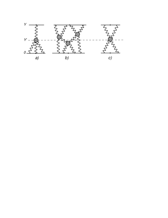
Figure 11: The vertex of one Pomeron to three Pomerons (Fig. 11-a); the contribution of the multi-Pomeron states (Fig. 11-b) and the first correction to the two Pomerons state (Fig. 11-c). The wavy lines denote the Green function of the dressed Pomeron.

In Fig. 11 the wavy lines denote the dressed Pomeron Green function ($G$), which is proportional to $Y^{-5}$ or to $Y^{-6}$ depending on the model. Therefore, the contribution of the diagram of Fig. 11-a is equal to

$$A_{13}\,\, \propto \,\int dY^{\prime}\,\Gamma\left(1\to 3\right)G\left(Y-Y^{\prime}\right)\,G^{3}\left(Y^{\prime}\right)$$

$$\rightarrow \,\Gamma\left(1\to 3\right)\int dY^{\prime}\left(Y-Y^{\prime}\right)^{-5}\,Y^{\prime-15}\propto\Gamma\left(1\to 3\right)Y^{-5}\propto G\left(Y\right)$$

One can see that the new vertex $\Gamma\left(1\to 3\right)$ led to the renormalization of the coupling of the Pomeron with the dipole, that is included in Eq. (1.1) in the term $S_{E}$. In other words, the new vertex did not change the BFKL Pomeron calculus.

The multi-gluon state, i.e. 2$n$-gluons in the $t$ channel, generates a larger intercept, than the intercept that the corresponding number ($n$) Pomerons would generate. As shown in Ref. [19], the new intercept can be calculated by summing the Pomeron exchanges, with the new vertex of the interaction of two Pomerons (see Fig. 11-b). The contribution of the first diagram shown in Fig. 11-c is equal to

$$A_{22}\, \propto \,\int dY^{\prime}\,\Gamma\left(2\to 2\right)G^{2}\left(Y-Y^{\prime}\right)\,G^{2}\left(Y^{\prime}\right)$$

$$\rightarrow \,\Gamma\left(2\to 2\right)\int dY^{\prime}\left(Y-Y^{\prime}\right)^{-10}\,Y^{\prime-10}\propto\Gamma\left(2\to 2\right)Y^{-10}\propto G^{2}\left(Y\right)\,\ll\,G\left(Y\right)$$

Therefore, the contribution of the multi -Pomeron exchanges with the interaction between them leads to small, negligible contributions.

In light of this, we conclude that the correction to the BFKL Pomeron calculus cannot change the fact that the total cross section falls at high energy. Of course, we have discussed only those multi-gluon states in the $t$ - channel, where each pair of gluons is in a colourless state. These states have been discussed in Ref.[19]. As far as we know, this is the only known example of the source of the intercept, which is larger than the intercept of the exchange of several Pomerons. Unfortunately, we do not know about the situation with the exchange of more general $n$-gluon states, which could make the BFKL Pomeron calculus incorrect in the $1/N_{c}$ approximation.However, the examples of such states have not been found ( see Ref. [37]).

We would like to recall, that the final re-summation was applied in the case of two extreme models, for the $\nu$ dependence of the 1 Pomeron $\to$ $n$ Pomerons transition vertices. The answer to this problem, is the next challenging problem which we hope to resolve in the near future.

Nevertheless, we believe that the problem addressed in this paper, is the first to be solved in order to start a theoretical discussion on what could happen with the dilute-dilute system of scattering, at high energy. Observing the substantial difference between the Pomeron self-energy and its Green function, we conclude that the quantum effects due to the BFKL Pomeron interaction, change the character of the asymptotic behaviour. Since these effects are so strong, they have to be taken into account for dilute-dense and dense-dense scattering, at ultra high energies.

5 Acknowledgements

This research was supported by the Fundaç$\tilde{a}$o para ci$\acute{e}$ncia e a tecnologia (FCT), and CENTRA - Instituto Superior T$\acute{e}$cnico (IST), Lisbon and by the Fondecyt (Chile) grant 1100648. One of us (JM) would like to thank Tel Aviv University for their hospitality on this visit, during the time of the writing of this paper.

6 Appendix A - The BFKL kernel and the triple Pomeron vertex

The BFKL kernel $\omega\left(\nu\right)$ is defined as

$$\omega\left(\nu\right)\hskip 8.5359pt=\hskip 8.5359pt\bar{\alpha}_{s}\chi\left(\nu\right)\,;\hskip 85.35826pt\,\left(\,\bar{\alpha}_{s}\hskip 8.5359pt=\hskip 8.5359pt\frac{\alpha_{s}N_{c}}{\pi}\,\right)$$ (A.1)

$$\chi\left(\nu\right)\hskip 8.5359pt=\hskip 8.5359pt\Re\left(\psi\left(1\right)-\psi\left(\frac{1}{2}+i\nu\right)\right)\hskip 8.5359pt=\hskip 8.5359pt2\psi\left(1\right)-\psi\left(\frac{1}{2}+i\nu\right)-\psi\left(\frac{1}{2}-i\nu\right)$$ (A.2)

where $\psi\left(x\right)$ is the Di-Gamma function, defined as [33]:

$$\psi\left(x\right)\hskip 8.5359pt =\hskip 8.5359pt\frac{d}{dx}\ln\Gamma\left(x\right)\hskip 8.5359pt=\hskip 8.5359pt-\,\gamma_{E}-\sum^{\infty}_{k=0}\left(\frac{1}{x+k}-\frac{1}{1+k}\right)$$ (A.3)

In the vicinity of $\nu\to 0$, the BFKL kernel takes the following form

$$\omega\left(\nu\right)\hskip 8.5359pt=\,\,\,\,4\bar{\alpha}_{s}\,\ln 2-14\bar{\alpha}_{s}\zeta\left(3\right)\nu^{2}\,\,=\,\,\omega\left(0\right)\,\,-\,\,D\nu^{2}\,\,\equiv\,\,\omega_{0}\,\,-\,\,D\nu^{2}$$ (A.4)

The planar vertex

The triple Pomeron vertex $\Gamma\left(\nu\,|\,\nu_{1},\nu_{2}\right)$ was defined above in Eq. (2.12), in terms of two contributing diagrams, namely the planar and non-planar diagrams shown in Fig. 3. The expression for the planar diagram given in Eq. (2.13), contained the function $\Omega\left(\nu|\nu_{1},\nu_{2}\right)$, which is given by the following integral (for a detailed explanation and derivation of these results, see Ref. [34]):

$$\Omega\left(\nu|\nu_{1},\nu_{2}\right)=\!\!\int\frac{d^{2}z_{0}d^{2}z_{1}d^{2}z_{2}}{\mid z_{01}z_{12}z_{20}\mid^{2}}\!\!\left(\frac{z_{01}}{z_{0}z_{1}}\frac{\bar{z_{01}}}{\bar{z}_{0}\bar{z}_{1}}\right)^{\!{\frac{1}{2}}+i\nu}\!\!\!\left(\frac{z_{12}}{\left(1-z_{1}\right)\left(1-z_{2}\right)}\!\frac{\bar{z}_{12}}{\left(1-\bar{z}_{1}\right)\left(1-\bar{z}_{2}\right)}\right)^{\!{\frac{1}{2}}+i\nu_{1}}\!\!\!\biggl{(}z_{20}\bar{z}_{20}\biggr{)}^{\!{\frac{1}{2}}+i\nu_{2}}\hskip 25.6073pt$$ (A.5)

The integrations of Eq. (A.5) were evaluated in [34], where the following results were derived. Note that in the original paper of ref. [34], the symmetric property $\Omega\left(\nu_{1}\,|\,\nu_{2},\nu_{3}\right)\,=\,\Omega\left(\nu_{3}\,|\,\nu_{1},\nu_{2}\right)\,=\,\Omega\left(\nu_{2}\,|\,\nu_{3},\nu_{1}\right)$ was derived. We have used this symmetric property, and hence the version of the function $\Omega$ written below is based on a different permutation of arguments and differs from the version given in ref. [34].

$$\Omega\left(\nu\,|\,\nu_{1},\nu_{2}\right)\hskip 8.5359pt=\hskip 8.5359pt\Omega_{1}\left(\nu\,|\,\nu_{1},\nu_{2}\right)\hskip 8.5359pt+\hskip 8.5359pt\Omega_{2}\left(\nu\,|\,\nu_{1},\nu_{2}\right)\hskip 8.5359pt+\hskip 8.5359pt\Omega_{3}\left(\nu\,|\,\nu_{1},\nu_{2}\right)$$ (A.6)

$$\Omega_{1}\left(\nu\,|\,\nu_{1},\nu_{2}\right)\hskip 8.5359pt=\hskip 8.5359pt\pi^{3}\,\,\frac{\Gamma\biggl{(}{\frac{1}{2}}+i\nu_{1}+i\nu_{2}-i\nu\biggr{)}}{\Gamma\biggl{(}{\frac{1}{2}}-i\nu_{1}-i\nu_{2}+i\nu\biggr{)}}\,\,\frac{\Gamma^{2}\biggl{(}{\frac{1}{2}}-i\nu_{1}\biggr{)}\Gamma^{2}\biggl{(}{\frac{1}{2}}-i\nu_{2}\biggr{)}}{\Gamma^{2}\biggl{(}{\frac{1}{2}}-i\nu\biggr{)}}$$ (A.7)

$$\times\,{{\int}}^{1}_{0}dx\left(1-x\right)^{-{\frac{1}{2}}-i\nu}\,\,_{2}F_{1}\left(\frac{1}{2}+i\nu_{1},\frac{1}{2}-i\nu_{1}\begin{vmatrix}1\end{vmatrix}x\right)\,_{2}F_{1}\left(\frac{1}{2}+i\nu_{2},\frac{1}{2}-i\nu_{2}\begin{vmatrix}1\end{vmatrix}x\right)$$

$$\times\,{{\int}}^{1}_{0}dy\,y^{-{\frac{1}{2}}-i\nu}\left(1-y\right)^{-{\frac{1}{2}}-i\nu_{1}-i\nu_{2}+i\nu}\,\,_{2}F_{1}\biggl{(}\frac{1}{2}-i\nu_{1},\frac{1}{2}-i\nu_{1}\begin{vmatrix}1\end{vmatrix}y\biggr{)}\,_{2}F_{1}\biggl{(}\frac{1}{2}-i\nu_{2},\frac{1}{2}-i\nu_{2}\begin{vmatrix}1\end{vmatrix}y\biggr{)}$$

$$\Omega_{2}\left(\nu\,|\,\nu_{1},\nu_{2}\right)\hskip 8.5359pt=\hskip 8.5359pt\pi^{3}\,\,\frac{\Gamma\biggl{(}{\frac{1}{2}}+i\nu_{1}+i\nu_{2}-i\nu\biggr{)}}{\Gamma\biggl{(}{\frac{1}{2}}-i\nu_{1}-i\nu_{2}+i\nu\biggr{)}}\,\,\frac{\Gamma\biggl{(}{\frac{1}{2}}+i\nu\biggr{)}\Gamma\biggl{(}{\frac{1}{2}}-i\nu\biggr{)}\Gamma\biggl{(}{\frac{1}{2}}-i\nu_{1}\biggr{)}\Gamma^{2}\biggl{(}{\frac{1}{2}}-i\nu_{2}\biggr{)}}{\Gamma\biggl{(}{\frac{1}{2}}+i\nu_{1}\biggr{)}}\hskip 28.45274pt$$ (A.8)

$$\times\,\underline{\,{}_{4}F_{3}\biggl{(}{\frac{1}{2}}+i\nu_{2},{\frac{1}{2}}-i\nu_{2},{\frac{1}{2}}-i\nu,{\frac{1}{2}}-i\nu\begin{vmatrix}1,1+i\nu_{1}-i\nu,1-i\nu_{1}-i\nu\end{vmatrix}1\biggr{)}}$$

$$\hskip 85.35826pt\Gamma\biggl{(}1+i\nu_{1}-i\nu\biggr{)}\Gamma\biggl{(}1-i\nu_{1}-i\nu\biggr{)}$$

$$\times\,{{\int}}^{1}_{0}dx\,\left(1-x\right)^{-{\frac{1}{2}}-i\nu_{1}-i\nu_{2}+i\nu}\,\,_{2}F_{1}\biggl{(}{\frac{1}{2}}-i\nu_{1},{\frac{1}{2}}-i\nu_{1}\begin{vmatrix}1\end{vmatrix}x\biggr{)}\,_{2}F_{1}\biggl{(}{\frac{1}{2}}-i\nu_{2},{\frac{1}{2}}-i\nu_{2}\begin{vmatrix}1\end{vmatrix}x\biggr{)}$$

$$\Omega_{3}\left(\nu\,|\,\nu_{1},\nu_{2}\right)\hskip 8.5359pt=\hskip 8.5359pt\Omega_{2}\left(\nu\,|\,\nu_{2},\nu_{1}\right)\hskip 14.22636pt$$ (A.9)

Using the following identity for the Hyper-geometric function (see Ref.[33] formula 9.100)

$$\,{}_{2}F_{1}\left(\,a,b\,\begin{vmatrix}c\end{vmatrix}x\right)\hskip 8.5359pt=\hskip 8.5359pt\left(1-x\right)^{c-a-b}\,_{2}F_{1}\left(c-a,c-b\begin{vmatrix}c\end{vmatrix}x\right)$$ (A.10)

then the factor $\,{}_{2}F_{1}\left({\frac{1}{2}}-i\nu_{1},{\frac{1}{2}}-i\nu_{1}\begin{vmatrix}1\end{vmatrix}x\right)\,_{2}F_{1}\left({\frac{1}{2}}-i\nu_{2},{\frac{1}{2}}-i\nu_{2}\begin{vmatrix}1\end{vmatrix}x\right)$ that appears in Eqs. (A.7) and (A.8) may be re-written, such that:

$$\Omega_{1}\left(\nu\,|\,\nu_{1},\nu_{2}\right)\hskip 8.5359pt=\hskip 8.5359pt\pi^{3}\,\,\frac{\Gamma\biggl{(}{\frac{1}{2}}+i\nu_{1}+i\nu_{2}-i\nu\biggr{)}}{\Gamma\biggl{(}{\frac{1}{2}}-i\nu_{1}-i\nu_{2}+i\nu\biggr{)}}\,\,\frac{\Gamma^{2}\biggl{(}{\frac{1}{2}}-i\nu_{1}\biggr{)}\Gamma^{2}\biggl{(}{\frac{1}{2}}-i\nu_{2}\biggr{)}}{\Gamma^{2}\biggl{(}{\frac{1}{2}}-i\nu\biggr{)}}$$ (A.11)

$$\times\,{{\int}}^{1}_{0}dx\left(1-x\right)^{-{\frac{1}{2}}-i\nu}\,\,_{2}F_{1}\left(\frac{1}{2}+i\nu_{1},\frac{1}{2}-i\nu_{1}\begin{vmatrix}1\end{vmatrix}x\right)\,_{2}F_{1}\left(\frac{1}{2}+i\nu_{2},\frac{1}{2}-i\nu_{2}\begin{vmatrix}1\end{vmatrix}x\right)$$

$$\times\,{{\int}}^{1}_{0}dy\,y^{-{\frac{1}{2}}-i\nu}\left(1-y\right)^{-{\frac{1}{2}}+i\nu_{1}+i\nu_{2}+i\nu}\,\,_{2}F_{1}\biggl{(}\frac{1}{2}+i\nu_{1},\frac{1}{2}+i\nu_{1}\begin{vmatrix}1\end{vmatrix}y\biggr{)}\,_{2}F_{1}\biggl{(}\frac{1}{2}+i\nu_{2},\frac{1}{2}+i\nu_{2}\begin{vmatrix}1\end{vmatrix}y\biggr{)}$$

$$\Omega_{2}\left(\nu\,|\,\nu_{1},\nu_{2}\right)\hskip 8.5359pt=\hskip 8.5359pt\pi^{3}\,\,\frac{\Gamma\biggl{(}{\frac{1}{2}}+i\nu_{1}+i\nu_{2}-i\nu\biggr{)}}{\Gamma\biggl{(}{\frac{1}{2}}-i\nu_{1}-i\nu_{2}+i\nu\biggr{)}}\,\,\frac{\Gamma\biggl{(}{\frac{1}{2}}+i\nu\biggr{)}\Gamma\biggl{(}{\frac{1}{2}}-i\nu\biggr{)}\Gamma\biggl{(}{\frac{1}{2}}-i\nu_{1}\biggr{)}\Gamma^{2}\biggl{(}{\frac{1}{2}}-i\nu_{2}\biggr{)}}{\Gamma\biggl{(}{\frac{1}{2}}+i\nu_{1}\biggr{)}}\hskip 28.45274pt$$ (A.12)

$$\times\,\underline{\,{}_{4}F_{3}\biggl{(}{\frac{1}{2}}+i\nu_{2},{\frac{1}{2}}-i\nu_{2},{\frac{1}{2}}-i\nu,{\frac{1}{2}}-i\nu\begin{vmatrix}1,1+i\nu_{1}-i\nu,1-i\nu_{1}-i\nu\end{vmatrix}1\biggr{)}}$$

$$\hskip 85.35826pt\Gamma\biggl{(}1+i\nu_{1}-i\nu\biggr{)}\Gamma\biggl{(}1-i\nu_{1}-i\nu\biggr{)}$$

$$\times\,{{\int}}^{1}_{0}dx\,\left(1-x\right)^{-{\frac{1}{2}}+i\nu_{1}+i\nu_{2}+i\nu}\,\,_{2}F_{1}\biggl{(}{\frac{1}{2}}+i\nu_{1},{\frac{1}{2}}+i\nu_{1}\begin{vmatrix}1\end{vmatrix}x\biggr{)}\,_{2}F_{1}\biggl{(}{\frac{1}{2}}+i\nu_{2},{\frac{1}{2}}+i\nu_{2}\begin{vmatrix}1\end{vmatrix}x\biggr{)}$$

$$\Omega_{3}\left(\nu\,|\,\nu_{1},\nu_{2}\right)\hskip 8.5359pt=\hskip 8.5359pt\Omega_{2}\left(\nu\,|\,\nu_{2},\nu_{1}\right)\hskip 14.22636pt$$ (A.13)

Using the following expansions for the Hyper-geometric functions (see Ref.[33] formulae 9.100 and 9.14):

$$\,{}_{2}F_{1}\left(a,b\,\begin{vmatrix}c\end{vmatrix}x\right)\hskip 8.5359pt=\hskip 8.5359pt\frac{\Gamma\left(c\right)}{\Gamma\left(a\right)\Gamma\left(b\right)}\sum^{\infty}_{n=0}\frac{\Gamma\left(a+n\right)\Gamma\left(b+n\right)}{\Gamma\left(c+n\right)}\frac{x^{n}}{n!}$$ (A.14)

$$\,{}_{4}F_{3}\left(a,b,c,d\,\begin{vmatrix}f,g,h\end{vmatrix}x\right)\hskip 8.5359pt=\hskip 8.5359pt\frac{\Gamma\left(f\right)\Gamma\left(g\right)\Gamma\left(h\right)}{\Gamma\left(a\right)\Gamma\left(b\right)\Gamma\left(c\right)\Gamma\left(d\right)}\sum^{\infty}_{n=0}\frac{\Gamma\left(a+n\right)\Gamma\left(b+n\right)\Gamma\left(c+n\right)\Gamma\left(d+n\right)}{\Gamma\left(f+n\right)\Gamma\left(g+n\right)\Gamma\left(h+n\right)}\frac{x^{n}}{n!}\hskip 42.67912pt$$ (A.15)

Then Eqs. (A.11 - A.13) can be re-cast in the following form:

$$\Omega_{1}\left(\nu\,|\,\nu_{1},\nu_{2}\right)\hskip 8.5359pt=\hskip 8.5359pt\pi^{3}\,\,\frac{\Gamma\biggl{(}{\frac{1}{2}}+i\nu_{1}+i\nu_{2}-i\nu\biggr{)}}{\Gamma\biggl{(}{\frac{1}{2}}-i\nu_{1}-i\nu_{2}+i\nu\biggr{)}}\,\,\frac{\Gamma\left({\frac{1}{2}}-i\nu_{1}\right)\Gamma\left({\frac{1}{2}}-i\nu_{2}\right)}{\Gamma^{2}\left({\frac{1}{2}}-i\nu\right)\Gamma^{3}\left({\frac{1}{2}}+i\nu_{1}\right)\Gamma^{3}\left({\frac{1}{2}}+i\nu_{2}\right)}$$ (A.16)

$${{\sum}}^{\infty}_{m,n=0}\,\,\Gamma\left({\frac{1}{2}}+i\nu_{1}+m\right)\Gamma\left({\frac{1}{2}}-i\nu_{1}+m\right)\Gamma\left({\frac{1}{2}}+i\nu_{2}+n\right)\Gamma\left({\frac{1}{2}}-i\nu_{2}+n\right)\,\,\,\frac{B\left(m+n+1\,|\,{\frac{1}{2}}-i\nu\right)}{\Gamma^{2}\biggl{(}1+m\biggr{)}\Gamma^{2}\biggl{(}1+n\biggr{)}}$$

$${{\sum}}^{\infty}_{p,r=0}\,\,\Gamma^{2}\left({\frac{1}{2}}+i\nu_{1}+p\right)\Gamma^{2}\left({\frac{1}{2}}+i\nu_{2}+r\right)\,\,\frac{B\left({\frac{1}{2}}-i\nu+p+r\,|\,{\frac{1}{2}}+i\nu+i\nu_{1}+i\nu_{2}\right)}{\Gamma^{2}\biggl{(}1+p\biggr{)}\Gamma^{2}\biggl{(}1+r\biggr{)}}\,\,$$

$$\Omega_{2}\left(\nu\,|\,\nu_{1},\nu_{2}\right)\hskip 8.5359pt=\hskip 8.5359pt\pi^{3}\,\,\frac{\Gamma\biggl{(}{\frac{1}{2}}+i\nu_{1}+i\nu_{2}-i\nu\biggr{)}}{\Gamma\biggl{(}{\frac{1}{2}}-i\nu_{1}-i\nu_{2}+i\nu\biggr{)}}\,\,\frac{\Gamma\left({\frac{1}{2}}+i\nu\right)\Gamma\left({\frac{1}{2}}-i\nu_{1}\right)\Gamma\left({\frac{1}{2}}-i\nu_{2}\right)}{\Gamma\left({\frac{1}{2}}-i\nu\right)\Gamma^{3}\left({\frac{1}{2}}+i\nu_{1}\right)\Gamma^{3}\left({\frac{1}{2}}+i\nu_{2}\right)}$$ (A.17)

$$\times\hskip 8.5359pt{{\sum^{\infty}_{p=0}}}\,\,\,\frac{\Gamma\left({\frac{1}{2}}+i\nu_{2}+p\right)\Gamma\left({\frac{1}{2}}-i\nu_{2}+p\right)\Gamma^{2}\left({\frac{1}{2}}-i\nu+p\right)}{\Gamma\biggl{(}1-i\nu+i\nu_{1}+p\biggr{)}\Gamma\biggl{(}1-i\nu-i\nu_{1}+p\biggr{)}}\frac{1}{\Gamma^{2}\biggl{(}1+p\biggr{)}}$$

$$\times\,\hskip 8.5359pt{{\sum^{\infty}_{m,n=0}}}\,\,\,\Gamma^{2}\left({\frac{1}{2}}+i\nu_{1}+m\right)\Gamma^{2}\left({\frac{1}{2}}+i\nu_{2}+n\right)\frac{B\left(1+m+n\,|\,{\frac{1}{2}}+i\nu+i\nu_{1}+i\nu_{2}\right)}{\Gamma^{2}\biggl{(}1+m\biggr{)}\Gamma^{2}\biggl{(}1+n\biggr{)}}$$

$$\Omega_{3}\left(\nu\,|\,\nu_{1},\nu_{2}\right)\hskip 8.5359pt=\hskip 8.5359pt\Omega_{2}\left(\nu\,|\,\nu_{2},\nu_{1}\right)\hskip 14.22636pt$$ (A.18)

where $B\left(m\,|\,n\right)$ is the well known beta-function, defined as (see Ref.[33] formula 8.380):

$$B\left(m\,|\,n\right)\hskip 8.5359pt=\hskip 8.5359pt{{\int}}^{1}_{0}dx\,x^{m-1}\left(1-x\right)^{n-1}\hskip 8.5359pt=\hskip 8.5359pt\frac{\Gamma\left(m\right)\Gamma\left(n\right)}{\Gamma\left(m+n\right)}$$ (A.19)

In the region $\nu_{1}\to 0$ and $\nu_{2}\to 0$ we can simplify the expressions for the $\Omega_{i}$. All of the $\Omega_{i}$ contain a pole at $i/2-\nu-\nu_{1}-i\nu_{2}=0$. In vicinity of this pole:

$$B\left(n|\frac{1}{2}+i\nu+i\nu_{1}+i\nu_{2}\right)\,\,\rightarrow\,\,\frac{1}{\frac{1}{2}+i\nu+i\nu_{1}+i\nu_{2}}\,\,+\mbox{\{non singlular terms\}}$$ (A.20)

Using the limit of Eq. (A.20) we can calculate the residue of the pole at $i/2-\nu-\nu_{1}-i\nu_{2}=0$ of the function $\Omega_{2}\left(\nu\,|\,\nu_{1},\nu_{2}\,\right)\hskip 8.5359pt=\hskip 8.5359pt\Omega_{3}\left(\nu\,|\,\nu_{2},\nu_{1}\,\right)$, for the even narrower region where $\nu_{1}\to 0$ and $\nu_{2}\to 0$. In this approach, from Eq. (A.17) in this region, the residue is:

$${{\lim_{\begin{subarray}{c}i/2-\nu-\nu_{1}-i\nu_{2}\to 0\\ \nu_{1},\nu_{2}\to 0\end{subarray}}}}\hskip 8.5359pt\left(i/2-\nu-\nu_{1}-\nu_{2}\,\right)\,\Omega_{2}\left(\nu\,|\,\nu_{1},\nu_{2}\right)\hskip 8.5359pt=\hskip 8.5359pt4\pi^{3}\,\,\,_{4}F_{3}\left({\frac{1}{2}},{\frac{1}{2}},1,1\begin{vmatrix}1,{\frac{3}{2}},{\frac{3}{2}}\end{vmatrix}1\right)$$

$$\times\,\,\,{{\lim_{\begin{subarray}{c}\nu_{1},\nu_{2}\to 0\end{subarray}}}}\hskip 8.5359pt\,_{2}F_{1}\left({\frac{1}{2}}+i\nu_{1},{\frac{1}{2}}+i\nu_{1}\begin{vmatrix}1\end{vmatrix}1\right)\,_{2}F_{1}\left({\frac{1}{2}}+i\nu_{2},{\frac{1}{2}}+i\nu_{2}\begin{vmatrix}1\end{vmatrix}1\right)$$

$$=\hskip 8.5359pt{{\lim_{\begin{subarray}{c}\nu_{1},\nu_{2}\to 0\end{subarray}}}}\hskip 8.5359pt-\,\,\frac{\pi}{3\nu_{1}\nu_{2}}$$ (A.21)

The identical result is true for $\Omega_{3}\left(\nu\,|\,\nu_{1},\nu_{2}\right)$. Repeating this procedure we obtain that $\Omega_{1}\propto\left(\nu_{1}+\nu_{2}\right)\ll\Omega_{2}$. Thus in the region $i/2-\nu-\nu_{1}-i\nu_{2}=0$ when $\nu_{1},\nu_{2}\to 0$, then the function $\Omega\left(\nu\,|\,\nu_{1},\nu_{2}\right)\hskip 8.5359pt=\hskip 8.5359pt\sum^{3}_{i=1}\Omega_{i}\left(\nu\,|\,\nu_{1},\nu_{2}\right)$ tends to $-2\pi/3\nu_{1}\nu_{2}$, neglecting the contribution from $\Omega_{1}$. Inserting this into Eq. (2.13) leads to the result:

$${{\lim_{\begin{subarray}{c}i/2-\nu-\nu_{1}-i\nu_{2}\to 0\\ \nu_{1},\nu_{2}\to 0\end{subarray}}}}\hskip 8.5359pt\left(i/2-\nu-\nu_{1}-\nu_{2}\,\right)\,\Gamma_{\mbox{\footnotesize{planar}}}\left(\nu\,|\,\nu_{1},\nu_{2}\right)\hskip 8.5359pt=\hskip 8.5359pt{{\lim_{\begin{subarray}{c}i/2-\nu\to 0\\ \nu_{1},\nu_{2}\to 0\end{subarray}}}}\hskip 8.5359pt\frac{-2\,\pi\,\left(\frac{1}{2}+i\nu\right)^{2}}{3\nu_{1}\nu_{2}}$$ (A.22)

The non-planar vertex

The formula for the triple Pomeron vertex of Eq. (2.12) contained also the contribution of the non-planar diagram, given by Eq. (2.14). This expression included the function $\Lambda\left(\nu|\nu_{1},\nu_{2}\right)$ , which is given in terms of the following integral in ref. [34]:

$$\Lambda\left(\nu|\nu_{1},\nu_{2}\right)=\!\!{{\int}}\frac{d^{2}z_{0}d^{2}z_{1}}{\mid z_{01}\mid^{4}}\!\!\left(\frac{z_{01}\bar{z_{01}}}{z_{0}z_{1}\bar{z}_{0}\bar{z}_{1}}\right)^{\!{\frac{1}{2}}+i\nu}\!\!\!\left(\frac{z_{01}}{\left(1-z_{0}\right)\left(1-z_{1}\right)}\frac{\bar{z}_{01}}{\left(1-\bar{z}_{0}\right)\left(1-\bar{z}_{1}\right)}\right)^{{\frac{1}{2}}+i\nu_{1}}\!\!\!\biggl{(}z_{01}\bar{z}_{01}\biggr{)}^{{\frac{1}{2}}+i\nu_{2}}\hskip 19.91684pt$$ (A.23)

The integrations of Eq. (A.23) were evaluated in ref. [34], where the following result was derived:

$$\Lambda\left(\nu\,|\,\nu_{1},\nu_{2}\right)\hskip 8.5359pt=\hskip 8.5359pt2^{2i\nu+2i\nu_{1}+2i\nu_{2}-1}\,\pi^{2}\,\,\frac{\Gamma\biggl{(}{\frac{1}{2}}-i\nu\biggr{)}\Gamma\biggl{(}{\frac{1}{2}}-i\nu_{1}\biggr{)}\Gamma\biggl{(}{\frac{1}{2}}-i\nu_{2}\biggr{)}}{\Gamma\biggl{(}{\frac{1}{2}}+i\nu\biggr{)}\Gamma\biggl{(}{\frac{1}{2}}+i\nu_{1}\biggr{)}\Gamma\biggl{(}{\frac{1}{2}}+i\nu_{2}\biggr{)}}\,\,\hskip 142.26378pt$$ (A.24)

$$\times\frac{\Gamma\biggl{(}{\frac{1}{4}}+{\frac{1}{2}}\left(i\nu+i\nu_{1}+i\nu_{2}\right)\biggr{)}}{\Gamma\biggl{(}{\frac{3}{4}}-{\frac{1}{2}}\left(i\nu+i\nu_{1}+i\nu_{2}\right)\biggr{)}}\frac{\Gamma\biggl{(}{\frac{1}{4}}+{\frac{1}{2}}\left(i\nu+i\nu_{1}-i\nu_{2}\right)\biggr{)}}{\Gamma\biggl{(}{\frac{3}{4}}-{\frac{1}{2}}\left(i\nu+i\nu_{1}-i\nu_{2}\right)\biggr{)}}\,\,\frac{\Gamma\biggl{(}{\frac{1}{4}}+{\frac{1}{2}}\left(-i\nu+i\nu_{1}+i\nu_{2}\right)\biggr{)}}{\Gamma\biggl{(}{\frac{3}{4}}-{\frac{1}{2}}\left(-i\nu+i\nu_{1}+i\nu_{2}\right)\biggr{)}}\frac{\Gamma\biggl{(}{\frac{1}{4}}+{\frac{1}{2}}\left(i\nu-i\nu_{1}+i\nu_{2}\right)\biggr{)}}{\Gamma\biggl{(}{\frac{3}{4}}-{\frac{1}{2}}\left(i\nu-i\nu_{1}+i\nu_{2}\right)\biggr{)}}$$

Using the above expression it is easy to see that:

$${{\lim_{\begin{subarray}{c}i/2-\nu-\nu_{1}-i\nu_{2}\to 0\\ \nu_{1},\nu_{2}\to 0\end{subarray}}}}\hskip 8.5359pt\left(i/2-\nu-\nu_{1}-\nu_{2}\right)\,\Lambda\left(\nu\,|\,\nu_{1},\nu_{2}\right)\hskip 8.5359pt=\hskip 8.5359pt{{\lim_{\begin{subarray}{c}i/2-\nu-\nu_{1}-i\nu_{2}\to 0\\ \nu_{1},\nu_{2}\to 0\end{subarray}}}}\hskip 8.5359pt\frac{\pi^{2}}{2}\,\,\,\frac{\left(\frac{1}{2}+i\nu\right)}{\nu_{1}\nu_{2}}$$ (A.25)

Plugging this result into the definition of the non-planar diagram of Eq. (2.14), we can derive the non-planar diagram in the limit $i/2-\nu-\nu_{1}-i\nu_{2}\to 0$ where $\nu_{1},\nu_{2}\to 0$. Using the fact that $\lim_{i/2-\nu\to 0}\chi\left(\nu\right)\to 1/\left(\frac{1}{2}+i\nu\right)$ (see the definition of Eq. (A.2)), the asymptote is:

$${{\lim_{\begin{subarray}{c}i/2-\nu-\nu_{1}-i\nu_{2}\to 0\\ \nu_{1},\nu_{2}\to 0\end{subarray}}}}\hskip 8.5359pt\left(i/2-\nu-\nu_{1}-\nu_{2}\right)\,\Gamma_{\mbox{\footnotesize{nonplanar}}}\left(\nu\,|\,\nu_{1},\nu_{2}\right)\hskip 8.5359pt=\hskip 8.5359pt{{\lim_{\begin{subarray}{c}i/2-\nu\to 0\\ \nu_{1},\nu_{2}\to 0\end{subarray}}}}\hskip 8.5359pt\frac{\pi^{2}}{2}\,\,\,\frac{\left(\frac{1}{2}+i\nu\right)^{2}}{\nu_{1}\nu_{2}}$$ (A.26)

Finally, inserting the asymptotes of Eqs. (A.22) and (A.26) into Eq. (2.12), we can calculate $\tilde{\Gamma}\left(\nu\,|\,\nu_{1},\nu_{2}\right)\hskip 8.5359pt=\hskip 8.5359pt\left(i/2-\nu-\nu_{1}-\nu_{2}\right)\Gamma\left(\nu\,|\,\nu_{1},\nu_{2}\right)$ in the region $i/2-\nu-\nu_{1}-i\nu_{2}\to 0$ where $\nu_{1},\nu_{2}\to 0$ as:

$${{\lim_{\begin{subarray}{c}i/2-\nu-\nu_{1}-\nu_{2}\to 0\\ \nu_{1},\nu_{2}\to 0\end{subarray}}}}\hskip 8.5359pt\tilde{\Gamma}\left(\nu\,|\,\nu_{1},\nu_{2}\right)\hskip 8.5359pt=\hskip 8.5359pt{{\lim_{\begin{subarray}{c}i/2-\nu\to 0\\ \nu_{1},\nu_{2}\to 0\end{subarray}}}}\hskip 8.5359pt\,\frac{a\,\left(\frac{1}{2}+i\nu\right)^{2}}{\nu_{1}\nu_{2}}$$ (A.27)

$$\mbox{where}\hskip 14.22636pta\hskip 8.5359pt=\hskip 8.5359pt-\,\frac{16\bar{\alpha}_{s}^{2}}{N_{c}}\,\,\,\,\left(\hskip 8.5359pt\frac{2\pi}{3}\hskip 8.5359pt+\hskip 8.5359pt\frac{\pi^{3}}{N_{c}^{2}}\hskip 8.5359pt\right)$$ (A.28)

In terms of the variables $\left\{\,\,\lambda,\sigma,\Delta\,\,\right\}$ defined in Eq. (2.15), then Eq. (A.27) becomes:

$${{\lim_{\begin{subarray}{c}\lambda\to\sigma\\ \sigma\to 0\end{subarray}}}}\hskip 8.5359pt\tilde{\Gamma}\left(\lambda\,|\,\sigma,\Delta\right)\hskip 8.5359pt=\hskip 8.5359pt{{\lim_{\begin{subarray}{c}\lambda\to\sigma\\ \sigma\to 0\end{subarray}}}}\hskip 8.5359pt\,\,\,\frac{a\,\lambda^{2}}{\left(\lambda+\Delta\right)\left(\lambda-\Delta\right)}$$ (A.29)

References

- [1] L. V. Gribov, E. M. Levin and M. G. Ryskin, Phys. Rep. 100, 1 (1983).
- [2] A. H. Mueller and J. Qiu, Nucl. Phys.,427 B 268 (1986) .
- [3] L. McLerran and R. Venugopalan, Phys. Rev. D 49,2233, 3352 (1994); D 50,2225 (1994); D 53,458 (1996); D 59,09400 (1999).
- [4] J. Jalilian-Marian, A. Kovner, A. Leonidov and H. Weigert, Phys. Rev. D59, 014014 (1999), [arXiv:hep-ph/9706377]; Nucl. Phys. B504, 415 (1997), [arXiv:hep-ph/9701284]; J. Jalilian-Marian, A. Kovner and H. Weigert, Phys. Rev. D59, 014015 (1999), [arXiv:hep-ph/9709432]; A. Kovner, J. G. Milhano and H. Weigert, Phys. Rev. D62, 114005 (2000), [arXiv:hep-ph/0004014] ; E. Iancu, A. Leonidov and L. D. McLerran, Phys. Lett. B510, 133 (2001); [arXiv:hep-ph/0102009]; Nucl. Phys. A692, 583 (2001), [arXiv:hep-ph/0011241]; E. Ferreiro, E. Iancu, A. Leonidov and L. McLerran, Nucl. Phys. A703, 489 (2002), [arXiv:hep-ph/0109115]; H. Weigert, Nucl. Phys. A703, 823 (2002), [arXiv:hep-ph/0004044].
- [5] I. Balitsky, [arXiv:hep-ph/9509348]; Phys. Rev. D60, 014020 (1999) [arXiv:hep-ph/9812311]
- [6] Y. V. Kovchegov, Phys. Rev. D60, 034008 (1999), [arXiv:hep-ph/9901281].
- [7] A. H. Mueller, A. I. Shoshi, S. M. H. Wong, Nucl. Phys. B715 (2005) 440-460. [hep-ph/0501088].
- [8] E. Levin, M. Lublinsky, Nucl. Phys. A763 (2005) 172-196. [hep-ph/0501173].
- [9] E. Iancu, D. N. Triantafyllopoulos, Nucl. Phys. A756 (2005) 419-467. [hep-ph/0411405].
- [10] A. Kovner, M. Lublinsky, Phys. Rev. D71 (2005) 085004. [hep-ph/0501198].
- [11] Y. Hatta, E. Iancu, L. McLerran, A. Stasto, D. N. Triantafyllopoulos, Nucl. Phys. A764 (2006) 423-459. [hep-ph/0504182].
- [12] M. A. Braun, Phys. Lett. B632 (2006) 297 [arXiv:hep-ph/0512057]; arXiv:hep-ph/0504002 ; Eur. Phys. J. C 33 (2004) 113 [arXiv:hep-ph/0309293]; Eur. Phys. J. C16, 337 (2000) [arXiv:hep-ph/0001268]; Phys. Lett. B483 (2000) 115-123 [hep-ph/0003004] [hep-ph/0504002]; Phys. Lett. B 483 (2000) 115 [arXiv:hep-ph/0003004]; Eur. Phys. J. C6, 321 (1999) [arXiv:hep-ph/9706373]; M. A. Braun, Phys. Lett. B483 (2000) 115-123 [hep-ph/0003004] [hep-ph/0504002]; Phys. Lett. B632 (2006) 297-304. [hep-ph/0512057];
- [13] T. Altinoluk, A. Kovner, M. Lublinsky, J. Peressutti, JHEP 0903 (2009) 109. [arXiv:0901.2559 [hep-ph]].
- [14] E. Levin, J. Miller, A. Prygarin, Nucl. Phys. A806 (2008) 245-286. [arXiv:0706.2944 [hep-ph]].
- [15] A. Kormilitzin, E. Levin, J. S. Miller, Nucl. Phys. A859 (2011) 87-113. [arXiv:1009.1329 [hep-ph]].
- [16] E. A. Kuraev, L. N. Lipatov, and F. S. Fadin, Sov. Phys. JETP 45, 199 (1977); Ya. Ya. Balitsky and L. N. Lipatov, Sov. J. Nucl. Phys. 28, 22 (1978).
- [17] J. Bartels, M. Braun and G. P. Vacca, Eur. Phys. J. C40, 419 (2005) [arXiv:hep-ph/0412218] ; J. Bartels and C. Ewerz, JHEP 9909, 026 (1999) [arXiv:hep-ph/9908454] ; J. Bartels and M. Wusthoff, Z. Phys. C66, 157 (1995) ; A. H. Mueller and B. Patel, Nucl. Phys. B425, 471 (1994) [arXiv:hep-ph/9403256]; J. Bartels, Z. Phys. C60, 471 (1993).
- [18] M. Kozlov, E. Levin, A. Prygarin, Nucl. Phys. A792, 122-151 (2007). [arXiv:0704.2124 [hep-ph]].
- [19] E. Laenen, E. Levin and A. G. Shuvaev, Nucl. Phys. B 419, 39 (1994); J, Bartels, Phys. Lett. B 298, 204,(1993); E. Levin, M. G. Ryskin and A. C. Shuvaev, , Nucl. Phys. B 387, 589 (1992).
- [20] A. H. Mueller and B. Patel, Nucl. Phys. B425, 471 (1994); A. H. Mueller and G. P. Salam, Nucl. Phys. B475, 293 (1996), [arXiv:hep-ph/9605302]; G. P. Salam, Nucl. Phys. B461, 512 (1996); E. Iancu and A. H. Mueller, Nucl. Phys. A730 (2004) 460, 494, [arXiv:hep-ph/0308315],[arXiv:hep-ph/0309276].
- [21] V. Alessandrini, D. Amati, R. Jengo, Nucl. Phys. B108 (1976) 425.
- [22] D. Amati, M. Le Bellac, G. Marchesini, M. Ciafaloni, Nucl. Phys. B112 (1976) 107.
- [23] M. Ciafaloni, M. Le Bellac, G. C. Rossi, Nucl. Phys. B130 (1977) 388.
- [24] M. Ciafaloni, Nucl. Phys. B146 (1978) 427.
- [25] S. Bondarenko, L. Motyka, A. H. Mueller, A. I. Shoshi, B. -W. Xiao, Eur. Phys. J. C50, 593-601 (2007). [hep-ph/0609213].
- [26] H. Navelet and R. B. Peschanski, Nucl. Phys. B 634 (2002) 291 [arXiv:hep-ph/0201285].
- [27] H. Navelet and R. B. Peschanski, Phys. Rev. Lett. 82 (1999) 1370 [arXiv:hep-ph/9809474].
- [28] A. Bialas, H. Navelet and R. B. Peschanski, Phys. Lett. B 427 (1998) 147 [arXiv:hep-ph/9711236].
- [29] M. Kozlov and E. Levin, Nucl. Phys. A 739, 291 (2004) [arXiv:hep-ph/0401118].
- [30] L. N. Lipatov, Phys. Rept. 286 (1997) 131-198. [hep-ph/9610276].
- [31] M. A. Braun, Eur. Phys. J. C 63 (2009) 287 [arXiv:0901.3660 [hep-ph]].
- [32] A. H. Mueller, Nucl. Phys. B 437 (1995) 107 [arXiv:hep-ph/9408245]; E. Levin, M. Lublinsky, Nucl. Phys. A730, 191-211 (2004). [hep-ph/0308279].
- [33] I. Gradstein and I. Ryzhik, ”Tables of Integrals, Seriee and Products”, Academic Press, 200..
- [34] G. P. Korchemsky, Nucl. Phys. B 550 (1999) 397 [arXiv:hep-ph/9711277].
- [35] H. Navelet and R. B. Peschanski, Nucl. Phys. B 634 (2002) 291 [arXiv:hep-ph/0201285]. (Eq. (A2) and Eq. (A17) )
- [36] http://en.wikipedia.org/wiki/Polylogarithm and references therein.
- [37] G. P. Korchemsky, , J.,Kotanski and A. N. Manashov,. Phys. Rev. Lett. 88 (2002) 122002, Phys. Lett. B 583 (2004) 121.