How Local is the Local Interstellar Magnetic Field?

Abstract

Similar directions are obtained for the local interstellar magnetic field (ISMF) by comparing diverse data and models that sample five orders of magnetic in spatial scales. These data include the ribbon of energetic neutral atoms discovered by the Interstellar Boundary Explorer, heliosphere models, the linear polarization of light from nearby stars, the Loop I ISMF, and pulsars that are within 100–300 pc. Together these data suggest that the local ISMF direction is correlated over scales of $\sim 100$ pc, such as would be expected for the interarm region of the galaxy.

1 Introduction

The properties of magnetic turbulence in interarm versus arm regions are distinctly different, as shown by Faraday rotation measure (RM) structure functions determined separately for the two regimes. The interstellar magnetic field (ISMF) is coherent over 100 pc scales in interarm regions, and random over spatial scales of less than 10 pc in arm regions Haverkorn:2006 . Which of these scenarios dominates for the ISMF in the solar vicinity? The heliosphere, and its ribbon of energetic neutral atoms (ENAs) discovered by the Interstellar Boundary Explorer (IBEX) spacecraft McComas:2009sci , probe the direction and strength of the very local ISMF in a single spatial location. Over intermediate scales, the position angles of starlight polarized by magnetically aligned interstellar dust grains trace the ISMF direction. Pulsar RM data give the field direction for spatial scales of 100–300 AU. As discussed in Frisch et al. Frisch:2011ismf2 , together these data and cosmic ray anisotropies suggest the ISMF near the Sun is similar to expectations for interarm regions.

2 IBEX Ribbon, Heliosphere, and Local ISMF

IBEX measures ENAs formed by charge-exchange (CEX) between heliospheric ions and neutral gas from the surrounding ISM, which flows through and around the heliosphere at a velocity of $\sim 26$ km s^-1 from the direction $\ell$,$b$$\sim 4^{\circ},15^{\circ}$. Among the sources of the ions creating the 0.01–6 keV ENAs detected by IBEX are the post-shock solar wind, pickup ions, and non-thermal energetic ions in the inner heliosheath, secondary ions created by CEX between interstellar protons and ENAs escaping beyond the heliopause, and possibly pickup ions inside of the solar wind termination shock. The first ENA full skymap, collected early 2009, revealed an unexpected ”ribbon” of ENAs that traces heliosphere asymmetries created by the angle between the ISMF and velocity of inflowing neutral interstellar gas (Fig. 1, McComas:2009sci, ; Funsten:2009sci, ; Schwadron:2009sci, ). The ribbon is visible in the energy range $\sim 0.2-6$ keV and forms a nearly complete circle in the sky, that is offset by $\sim 75^{\circ}$ from the ribbon arc center Schwadronetal:2011sep . Comparisons between heliosphere models (see below) and the ENA ribbon revealed that the ribbon is seen towards sightlines that are perpendicular to the ISMF draping over the heliosphere Schwadron:2009sci . Seven possible formation mechanisms for the ribbon have been discussed McComasetal:2010var ; Schwadronetal:2011sep ; McComas:2009sci ; GrzedzielskiBzowski:2010ribbon . In order to link the ribbon directly to the ISMF draping over the heliosphere, the mechanism based on CEX between interstellar H^∘ and energetic ions beyond the heliopause is assumed to be correct (Heerikhuisen:2010ribbon, ; Chalov:2010ribbon, ). The ribbon location is stable over the first several skymaps McComasetal:2010var . The ISMF direction at the heliosphere is then given by the center of the ribbon arc, located at $\ell$=33^∘, $b$=55^∘ (see Table 1 for ecliptic coordinates).

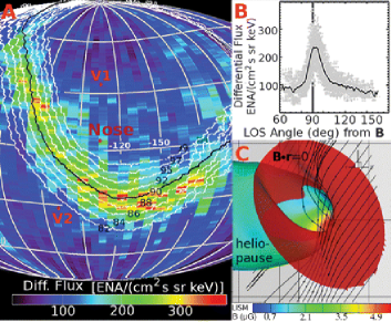
Figure 1: (A) Contours of constant angular offsets from the pole of the IBEX ribbon at $\lambda$=221^∘, $\beta$=39^∘, shown plotted against the IBEX 1 keV ENA fluxes. The black line shows the locus of points perpendicular to the ISMF direction, e.g. B$\cdot$R=0, based on the ISMF displayed in (C) from the heliosphere model of Pogorelovetal:2009asymmetries . B is the magnetic field vector and R is the radial sightline. Plot (B) shows the correlation between global 1 keV ENA fluxes and B$\cdot$R. Plot (A) is in ecliptic coordinates, and centered on the heliosphere nose. The locations of the two Voyager spacecraft are identified. The figure is from Schwadron:2009sci .

The best match between the predicted and observed ribbon locations occurs for ENAs produced roughly 100 AU beyond the heliopause HeerikhuisenPogorelov:2011 . The surrounding cloud is $\sim 22$% ionized ($n(\mathrm{p})\sim 0.07$ cm^-3, SlavinFrisch:2008, ). The ribbon formation mechanism requires that ENAs escaping the heliosphere CEX with interstellar protons piled up against the heliopause, creating a secondary pickup ion population in the outer heliosheath. The secondary pickup ion must CEX quickly with an interstellar H^∘ atom (before magnetic turbulence disrupts the ring-beam distribution), to create an ENA detected preferentially in directions perpendicular to the ISMF. The relative roles of large- and small-scale magnetic turbulence in the outer heliosheath are not presently understood, so this mechanism is still under study Florinski:2010ribbon ; GamayunovZhang:2010ribbon . A recent model HeerikhuisenPogorelov:2011 reproduces the ribbon for an ISMF strength of $\leq 3$ $\mu{\rm G}$, with the pole directed from $\ell$=33^∘, $b$=54^∘ (or $\lambda,\beta=222^{\circ},39^{\circ}$). A local ISMF strength of $\sim 3$ $\mu{\rm G}$ is found from photoionizaton models of the local interstellar cloud (LIC) around the heliosphere, and the assumption of pressure equilibrium between the ISMF and thermal gas SlavinFrisch:2008 .

MHD heliosphere models are constructed to reproduce the heliospere asymmetries induced by the $\sim 45^{\circ}$ angle between the ISMF direction and gas flow direction (Pogorelovetal:2009asymmetries, ; Prestedetal:2010, ; Opheretal:2007, ; Ratkiewiczetal:2008, ). The ISMF direction in these models is generally directed downwards through the ecliptic plane in order to reproduce asymmetries such as the $\sim 5^{\circ}$ offset between the central directions of the flows of interstellar H and He into the heliosphere, and the difference between the solar wind termination shock distances encountered by Voyager 1 (94 AU) versus Voyager 2 (84 AU).

If the IBEX ribbon is formed beyond the heliopause through CEX with secondary pickup ions, then the ribbon is an extraordinary diagnostic of the local ISMF and neutral densities. Models show that variations in interstellar properties of $\sim 15$% lead to pronounced differences in the location and width of the ribbon because of the interplay between magnetic, plasma and neutral pressures Frisch:2010next ; HeerikhuisenPogorelov:2011 .

Two aspects of the ribbon data are notable: (1) The imprint of the solar wind on ENA fluxes and the ribbon is apparent in flux decreases of $\sim 15$% between the first and second skymaps, spaced by six months McComasetal:2010var . The travel time for a 1 keV solar wind proton to pass the Earth, the solar wind termination shock, and then return to IBEX as an ENA, is over two years. This time lag suggests that the decrease in 0.7–1.1 keV fluxes in the second map is from the unusually low solar wind pressure of the recent solar cycle minimum. (2) The energy distribution of global ENAs shows an overall power law spectra, $E^{-\kappa}$, with $\kappa$ ranging between 1.28 and 2.04 for different regions of the sky and spectral intervals Funsten:2009sci . The power-law distribution of ribbon ENAs becomes softer above a ”knee” in the spectrum between 1–4 keV, which occurs at higher energies for higher latitudes Schwadronetal:2011sep .

3 Local ISMF direction from polarized starlight

The galactic ISMF was first mapped in the 1940’s using polarized starlight, which showed patterns of linear polarization related to dust extinction. In the diffuse ISM, dust grain alignment occurs when magnetic torques align asymmetric rotating charged dust grains, producing a birefringent interstellar medium with lowest opacities parallel to the ISMF direction. This gives linear polarization that is parallel to, and traces, the ISMF direction Roberge:2004 . For sightlines perpendicular to the ISMF direction in a uniform medium, polarization will increase with distance. Polarizations do not provide the strength or polarity of the ISMF, and polarization is reduced by foreshortening towards the poles of the field.

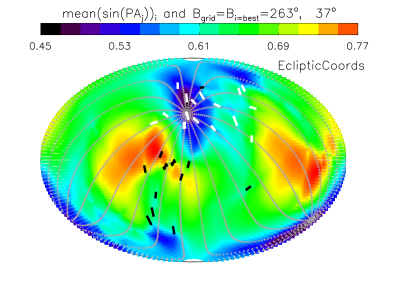
Figure 2: Best best-fitting ISMF direction from polarization data is determined by minimizing the function $<\sin(\mathrm{PA_{i}})>$. $\mathrm{PA_{i}}$ is the position angle of linear polarizations in the i^th possible ISMF direction. The mean is evaluated for data towards stars within 40 pc and 90^∘ of the heliosphere nose (where the G-cloud is seen, see Frisch:2010ismf ). Gray dots show the best fitting ISMF, which is directed towards $\lambda$=263^∘, $\beta$=37^∘, with uncertainties of $\sim\pm 35^{\circ}$ (corresponding to $\ell$,$b$=38^∘,23^∘). A new study using an extended polarization data set returns similar results for the local ISMF direction, but the uncertainties are larger Frisch:2011ismf2 . Polarization vectors are plotted with either black or white bars. The figure is from Frisch:2010ismf .

During the early 1970’s, Tinbergen Tinbergen:1982 conducted a sensitive (for that time) study of the interstellar polarizations of stars within $\sim 40$ pc of the Sun, and found a patch of dust in the south and close to the Sun. Based on interstellar absorption lines towards $\alpha$ Cen at 1.3 pc, and polarization towards 36 Oph, the magnetically aligned dust must be in the ”G-cloud” within 1.3 pc Frisch:2011araa . Recent polarization data confirm that local interstellar polarizations are significantly weaker in the northern hemisphere than the southern hemisphere.

We have analyzed available interstellar polarization data, including six recent sets of sensitive data, to determine the best fitting ISMF direction for a 180^∘ diameter region that is centered on the heliosphere nose and coinciding roughly with the G-cloud (Frisch:2010ismf ; Frisch:2011ismf2 . Although we utilize polarization towards stars out to 40 pc, most of the polarization should be formed in the region with the highest concentrations of gas within $\sim 15$ pc Frisch:2011araa ; Frisch:2011ismf2 . These data indicate a local ISMF direction with a pole towards $\ell$,$b$$\sim 38^{\circ},23^{\circ}$, with uncertainties of $\sim\pm 35^{\circ}$ (Fig. 2, Table 1, Frisch:2010ismf ; Frisch:2011ismf2 ). This direction is centered approximately 35^∘ from the center of the IBEX ribbon arc. The small difference between the two directions may indicate turbulence in the local ISMF, for example between the ISMF directions of the G-cloud (within 1.3 pc) and the LIC in which the Sun is embedded. In several regions, the flow of interstellar gas past the Sun shows merging or colliding clouds RLIV:2008vel , such as the two clouds in front of Sirius FrischMueller:2011ssr , which could drive local magnetic turbulence.

Scales	ISMF Source	Angle	$\lambda$, $\beta$	$\ell$,$b$
$\sim 150$ AU	IBEX ribbon center Funsten:2009sci	0∘	221∘, 39∘	33∘, 55∘
$\sim 150$ AU	Heliosphere model HeerikhuisenPogorelov:2011	3∘	224∘, 41∘	36∘, 53∘
$<40$ pc	Optical polarization Frisch:2010ismf ; Frisch:2011ismf2	32∘	263∘, 37∘	38∘, 23∘ ($\pm 35^{\circ}$)
80 pc	S1 Magnetic Bubble Wolleben:2007	$46^{+26}_{-22}$	291∘, 64∘	71∘, 18∘($\pm 48^{\circ}$)
150 pc	Pulsar RM data Salvati:2010	23∘	232∘, 18∘	5∘, 42∘

Table 1: Interstellar Magnetic Field Direction, 150 AU – 150 pc

4 The Loop I superbubble and local ISMF

Loop I is an evolved but reheated superbubble that dominates the northern hemisphere because of it’s large angular radius. It appears as a distinct imprint on the ISMF within 100 pc that is detected in polarized starlight, polarized radio continuum, Faraday rotation, and Zeeman splitting in the HI filaments defining the shell circumference Frisch:1995rev . All existing spherically symmetric models of the radio continuum Loop I place the Sun in the superbubble rim. A recent study of the intensity of 1.4 GHz emission in this region derived two subshells of Loop I containing enhanced synchrotron emissivity from swept up magnetic fields, and placing the Sun in the rim of the S1 subshell Wolleben:2007 ; Frisch:2010s1 . The direction of the bulk flow of the ”cluster of local interstellar clouds” (CLIC) past the Sun has an upwind direction of $\ell$,$b$=335^∘,–7^∘  (FrischMueller:2011ssr , after correcting for the solar velocity through the local standard of rest, LSR), near the center of the S1 shell,

If the CLIC is part of the nearside of an evolved superbubble shell associated with Loop I Frisch:1995rev ; Frisch:2011araa , then both the polarity and direction of the local ISMF could be ordered over the $\sim 78$ pc radius of the S1 subshell. The angle between the local ISMF direction and the LSR CLIC velocity is 68^∘–78^∘, depending on whether the comparison is with the polarization axis or ribbon arc center. This large angle suggests that the very local ISMF is roughly parallel to the local surface of the expanding Loop I shell.

5 ISMF from pulsars in the Local Bubble

The ratio of pulsar Faraday rotation measures (RM) and dispersion measures provides an electron-density weighted measurement of the ISMF component parallel to the sightline, and the field polarity. Salvati (2010) performed a best-fit to the rotation and dispersion measures of four pulsars within 160–300 pc, and in the very low density third galactic quadrant corresponding to the interior of the Local Bubble. He found a best-fit direction of $\ell$$\sim 5^{\circ}$, $b$$\sim 42^{\circ}$, and a field strength of $|B|$=3.3 $\mu{\rm G}$ (Table 1). This direction is within 23^∘ of the center of the IBEX ribbon arc, and 33^∘ of the best-fitting ISMF direction. The polarity of this ISMF is directed towards the pole of $\lambda$,$\beta$=232^∘,18^∘, indicating that it is directed upwards through the plane of the ecliptic. Wolleben Wolleben:2007 finds a similar RM polarity in this direction, although variations over small angular scales are seen.

6 Galactic cosmic rays and the local ISMF

An unusual indicator of the ISMF affecting the heliosphere is provided by GeV–TeV galactic cosmic rays (GCR). Cosmic rays at sub-TeV energies have gyroradii less than several hundred AU in a 1 $\mu{\rm G}$ magnetic field, which is comparable to heliosphere dimensions. GCRs with energies $\leq 10^{3}$ GeV show pronounced spatial asymmetries Nagashimaetal:1998 ; Halletal:1999gcr ; LazarianDesiati:2010 , including a sidereal distribution with a southern GCR deficit, and a broad excess emission region attributed to the heliotail. The broad tail-in excess at 500–1000 GeV is centered at ecliptic coordinates of $\lambda$,$\beta$ of 71^∘,–42^∘ to 90^∘,–53^∘, and is skewed with respect to ecliptic latitude and covers the direction opposite to the ISMF defined by the ribbon arc ($\lambda$,$\beta$=41^∘,–39^∘, Table 1). This tail-in excess also coincides with the axis of the ISMF determined from the polarization data, $\lambda$,$\beta$=83^∘,–37^∘. The minimum in tail ENA fluxes is 44^∘ west of the downwind gas-flow direction Schwadronetal:2011sep , and it overlaps the excess of sub-TeV particles. Evidently the GCR excess could form either in deep tail regions or indicate GCRs streaming along the local ISMF or S1 shell. Lazarian and Desiati (2010) have modeled the tail-in sub-TeV excess as due to the stochastic acceleration of particles in the time-variable magnetic field of the heliotail.

7 Summary

The summary of data in the previous sections shows that the direction of the ISMF appears to be relatively constant over scales of five orders of magnitude, with warping (large-scale turbulence) or variations in the field direction typically less than 30^∘–40^∘ (Table 1). The agreement between ISMF direction from pulsars in the Local Bubble, starlight polarizations, the IBEX ribbon, and heliosphere models, is remarkable considering that the spatial scales of these estimates differ by five orders of magnitude. The puzzle is that opposite polarities are inferred for the ISMF shaping the heliosphere and the pulsar RM data, downwards through the ecliptic plane in the first case and upwards through the ecliptic plane in the second case. It could be pure coincidence that the Local Bubble ISMF direction from the pulsar data and from heliosphere measurements and models are similar. However the galactic magnetic field is known to be ordered over kiloparsec spatial scales in low density interarm regions of the Galaxy such as around the Sun JinLinHan:2009 . Perhaps it is not so surprising to see uniformity of the magnetic field direction over local scales of 100 pc. If the ISMF traced by the IBEX ribbon, polarization data, Loop I shell, and pulsar data are related, it would mean that Loop I is a highly asymmetric evolved superbubble, with the Sun in the segment most distant from the superbubble source and most closely linked to the interarm field direction.

References

- (1) M. Haverkorn, B. M. Gaensler, J. C. Brown, N. S. Bizunok, N. M. McClure-Griffiths, J. M. Dickey, and A. J. Green, ApJ 637, L33–L35 (2006).
- (2) D. J. McComas, F. Allegrini, P. Bochsler, M. Bzowski, E. R. Christian, G. B. Crew, R. DeMajistre, H. Fahr, H. Fichtner, P. C. Frisch, H. O. Funsten, S. A. Fuselier, G. Gloeckler, M. Gruntman, J. Heerikhuisen, V. Izmodenov, P. Janzen, P. Knappenberger, S. Krimigis, H. Kucharek, M. Lee, G. Livadiotis, S. Livi, R. J. MacDowall, D. Mitchell, E. Möbius, T. Moore, N. V. Pogorelov, D. Reisenfeld, E. Roelof, L. Saul, N. A. Schwadron, P. W. Valek, R. Vanderspek, P. Wurz, and G. P. Zank, Science 326, 959– (2009).
- (3) P. C. Frisch, B. Andersson, A. Berdyugin, H. O. Funsten, M. Magalhaes, D. J. McComas, W. DeMajistre, V. Piirola, N. A. Schwadron, J. D. Slavin, and S. J. Wiktorowicz, in preparation (2011).
- (4) H. O. Funsten, F. Allegrini, G. B. Crew, R. DeMajistre, P. C. Frisch, S. A. Fuselier, M. Gruntman, P. Janzen, D. J. McComas, E. Möbius, B. Randol, D. B. Reisenfeld, E. C. Roelof, and N. A. Schwadron, Science 326, 964–967 (2009).
- (5) N. A. Schwadron, M. Bzowski, G. B. Crew, M. Gruntman, H. Fahr, H. Fichtner, P. C. Frisch, H. O. Funsten, S. Fuselier, J. Heerikhuisen, V. Izmodenov, H. Kucharek, M. Lee, G. Livadiotis, D. J. McComas, E. Moebius, T. Moore, J. Mukherjee, N. V. Pogorelov, C. Prested, D. Reisenfeld, E. Roelof, and G. P. Zank, Science 326, 966– (2009).
- (6) N. A. Schwadron, F. Allegrini, M. Bzowski, E. R. Christian, G. B. Crew, M. Dayeh, R. DeMajistre, et al., ApJ 731, 56–77 (2011).
- (7) D. J. McComas, M. Bzowski, P. C. Frisch, G. B. Crew, M. A. Dayeh, R. DeMajistre, H. O. Funsten, et al., J. Geophys. Res. 115, A09113 (2010).
- (8) S. Grzedzielski, M. Bzowski, A. Czechowski, H. O. Funsten, D. J. McComas, and N. A. Schwadron, ApJ 715, L84–L87 (2010).
- (9) J. Heerikhuisen, N. V. Pogorelov, G. P. Zank, G. B. Crew, P. C. Frisch, H. O. Funsten, P. H. Janzen, D. J. McComas, D. B. Reisenfeld, and N. A. Schwadron, ApJ 708, L126–L130 (2010).
- (10) S. V. Chalov, D. B. Alexashov, D. McComas, V. V. Izmodenov, Y. G. Malama, and N. Schwadron, ApJ 716, L99–L102 (2010).
- (11) N. V. Pogorelov, J. Heerikhuisen, J. J. Mitchell, I. H. Cairns, and G. P. Zank, ApJ 695, L31–L34 (2009).
- (12) J. Heerikhuisen, and N. V. Pogorelov, ApJ 738, 29 (2011).
- (13) J. D. Slavin, and P. C. Frisch, A&A 491, 53–68 (2008).
- (14) V. Florinski, G. P. Zank, J. Heerikhuisen, Q. Hu, and I. Khazanov, ApJ 719, 1097–1103 (2010).
- (15) K. Gamayunov, M. Zhang, and H. Rassoul, ApJ 725, 2251–2261 (2010).
- (16) C. Prested, M. Opher, and N. Schwadron, ApJ 716, 550–555 (2010).
- (17) M. Opher, E. C. Stone, and T. I. Gombosi, Science 316, 875– (2007).
- (18) R. Ratkiewicz, L. Ben-Jaffel, and J. Grygorczuk, “What Do We Know about the Orientation of the Local Interstellar Magnetic Field?,” in Numerical Modeling of Space Plasma Flows, edited by N. V. Pogorelov, E. Audit, and G. P. Zank, 2008, vol. 385 of Astro. Soc. of Pacific Conf. Ser., p. 189.
- (19) P. C. Frisch, J. Heerikhuisen, N. V. Pogorelov, B. DeMajistre, G. B. Crew, H. O. Funsten, P. Janzen, D. J. McComas, E. Moebius, H. Mueller, D. B. Reisenfeld, N. A. Schwadron, J. D. Slavin, and G. P. Zank, ApJ 719, 1984–1992 (2010).
- (20) W. G. Roberge, “Alignment of Interstellar Dust,” in Astrophysics of Dust, edited by A. N. Witt, G. C. Clayton, & B. T. Draine, 2004, vol. 309 of Astron. Soc. of Pacific Conf. Ser., p. 467.
- (21) P. C. Frisch, B. Andersson, A. Berdyugin, H. O. Funsten, M. Magalhaes, D. J. McComas, V. Piirola, N. A. Schwadron, J. D. Slavin, and S. J. Wiktorowicz, ApJ 724, 1473–1479 (2010).
- (22) J. Tinbergen, A&A 105, 53–64 (1982).
- (23) P. C. Frisch, S. Redfield, and J. Slavin, ARA&A 49, in press (2011).
- (24) S. Redfield, and J. L. Linsky, ApJ 673, 283–314 (2008).
- (25) P. C. Frisch, and H.-R. Mueller, Space Sci. Rev. p. 130 (2011).
- (26) M. Wolleben, ApJ 664, 349–356 (2007).
- (27) M. Salvati, A&A 513, A28+ (2010).
- (28) P. C. Frisch, Space Sci. Rev. 72, 499–592 (1995).
- (29) P. C. Frisch, ApJ 714, 1679–1688 (2010).
- (30) K. Nagashima, K. Fujimoto, and R. M. Jacklyn, J. Geophys. Res. 103, 17429–17440 (1998).
- (31) D. L. Hall, K. Munakata, S. Yasue, S. Mori, C. Kato, M. Koyama, S. Akahane, Z. Fujii, K. Fujimoto, J. E. Humble, A. G. Fenton, K. B. Fenton, and M. L. Duldig, J. Geophys. Res. 104, 6737–6750 (1999).
- (32) A. Lazarian, and P. Desiati, ApJ 722, 188–196 (2010).
- (33) J. Han, “The magnetic structure of our Galaxy: a review of observations,” 2009, vol. 259 of IAU Symposium, p. 455.