SuperCool Inflation: A Graceful Exit
from Eternal Inflation at LHC Scales and Below

Abstract

In SuperCool Inflation (SCI), a technically natural and thermal effect gives a graceful exit to old inflation. The Universe starts off hot and trapped in a false vacuum. The Universe supercools and inflates solving the horizon and flatness problems. The inflaton couples to a set of QCD like fermions. When the fermions’ non-Abelian gauge group freezes, the Yukawa terms generate a tadpole for the inflaton, which removes the barrier. Inflation ends, and the Universe rapidly reheats. The thermal effect is technically natural in the same way that the QCD scale is technically natural. In fact, Witten used a similar mechanism to drive the Electro-Weak (EW) phase transition; critically, no scalar field drives inflation, which allows SCI to avoid eternal inflation and the measure problem. SCI also works at scales, which can be probed in the lab, and could be connected to EW symmetry breaking. Finally, we introduce a light spectator field to generate density perturbations, which match the CMB. The light field does not affect the inflationary dynamics and can potentially generate non-Gaussianities and isocurvature perturbations observable with Planck.

I Introduction

In 1981, Guth Guth:1980zm introduced an inflationary phase (old inflation) to explain the horizon, flatness, and monopole problems. The Universe begins hot, cools, and becomes stuck in a false vacuum and begins to inflate. Eventually, the Universe transitions to the true vacuum and reheats. Unfortunately, Guth’s model failed due to the Swiss cheese problem or lack of a graceful exit. The tunneling rate to the true vacuum must be small to generate a sufficient amount of inflation, but then inflation never ends.

New inflation Linde:1981mu ; Albrecht:1982wi sidestepped the Swiss cheese problem by introducing a slowly rolling scalar field to drive inflation. Slow roll not only solves the standard cosmological problems but can also generate adiabatic density perturbations consistent with the CMB. Regardless, slow roll has two serious generic drawbacks beyond the fine-tuning problem Adams:1990pn ; first, the high scale of inflation (which prevents testing inflation in the lab) leads to problems from trans-Planckian physics to overclosure from moduli and gravitinos; second (a much worst problem), eternal inflation (which leads to the measure problem) undermines the predictive power of inflation. Hence, one is interested in alternatives to slow roll such as cyclic models and ekpyrotic Universes Khoury:2001wf , but these models must contend with a singular bounce, which introduces a different can of worms.

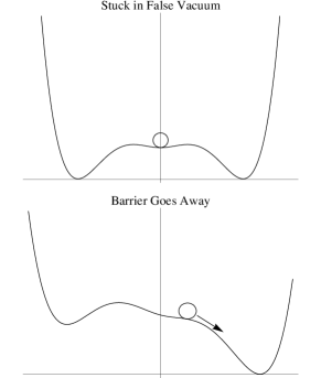
Figure 1: top– The Universe is stuck in a false vacuum and supercools. bottom– At T_c, a Yukawa term generates a tadpole term; the barrier goes away. The Universe then rapidly transitions to the true vacuum.

Instead, we do away with any scalar dynamics to control inflation. A thermal bath (present during old inflation) regulates inflation. We introduce a new thermal and technically natural mechanism to generate a graceful exit. We have dubbed the model SuperCool (SC) inflation since the Universe supercools during inflation and then rapidly transitions to the true vacuum due to a small perturbation, in much the same that a supercooled liquid almost instantaneously freezes if slightly disturbed. The model in spirit is similar to thermal inflation Lyth:1995ka except unlike thermal inflation our model successfully solves the cosmological problems and generates adiabatic density perturbations. SuperCool Inflation (SCI) works at the TeV scale and below and avoids eternal inflation.

For simplicity, SuperCool (SC) field is a complex scalar with a Coleman-Weinberg potential

$$V(\phi)=(1/8)\,\text{T}^{2}\,\phi^{2}+\frac{3g_{X}^{4}}{32\pi^{2}}|\phi|^{4}\bigg{(}\ln\bigg{(}\frac{|\phi|}{\langle|\phi|\rangle}\bigg{)}-\frac{1}{4}\bigg{)}$$ (1)

$$+\sum y_{i}\phi\ast(q_{R}\bar{q}_{L})_{i}+\text{h.c.}+\Lambda^{4}+\text{ non-renormalizable}$$

charged under a U(1)_X gauge group with a charge $g_{x}$, where $\Lambda^{4}$ is the standard cosmological tuning, which tunes the cosmological constant of the true vacuum to zero. Finite temperature effects generate an effective mass term (T${}^{2}\phi^{2}$). The SC field couples to a set of QCD like fermions $q_{R}\bar{q}_{L}$ with a Yukawa coupling $\lambda_{i}$. The SC sector is a simplified version of the standard model with the SC inflaton mapped to the Higgs boson. The SU(2) weak force accompanied by leptons has been dropped. The non-renormalizable terms will play an important role in avoiding eternal inflation.

We will discuss Eq. 1 in detail in the text but first describe the qualitative behavior of Eq. 1. In the beginning, the Universe is hot and dense, becomes stuck in a false vacuum (Fig. 1–top), and inflates solving the horizon and flatness problems. The temperature of the Universe falls exponentially. In section II.1, we show that finite temperature effects stabilize the potential against tunneling during inflation.

In section II.2, we introduce a technically natural way to end inflation. When the Universe reaches the critical temperature T_c, a non-Abelian gauge group freezes, which triggers the end of inflation. A set of QCD like fermions charged under the non-Abelian gauge group get a vev $\langle\lambda\bar{\lambda}\rangle\simeq$ T${}_{c}^{3}$. The fermions (which have a Yukawa coupling to the SC field) generate a tadpole term for the inflaton potential. The new term removes the barrier trapping the scalar field in the false vacuum (Fig. 1–bottom). We remind the reader that as the temperature of the Universe drops the barrier trapping the false becomes smaller; the barrier scales with T. The field then quickly rolls down to the true vacuum and reheats the Universe. The mechanism is technically natural; the end of inflation is determined by the logarithmic running of a non-Abelian gauge group. In the same way, the QCD scale is technically natural compared to the Planck scale, which is a difference of $10^{20}$ orders of magnitude and many orders of magnitude more than the temperature difference between when SC inflation begins and ends.

In the case of radiative Electro-Weak (EW) symmetry breaking, Weinberg and Guth Guth:1981uk noted that the Universe would become trapped in the symmetric false vacuum of the Higgs potential to arbitrarily low temperatures. Witten Witten:1980ez showed that when the QCD vacuum freezes, the Yukawa terms generate a tadpole term for the Higgs potential. The new term destabilizes the false vacuum and the Universe transitions to the true vacuum. We take Witten’s observation and introduce it as a way to generate a graceful exit for old inflation.

After the field goes to the true vacuum in section II.3, we show that the Universe rapidly reheats. We discuss the different ways that the inflaton can couple to the standard model. As an instructive example, we consider kinetic mixing between hypercharge U(1)_Y and U(1)_X which generates a $Z^{\prime}$. The SC inflaton then decays into a pair of Z bosons.

A high scale of inflation (order GUT) can be problematic. The GUT scale generically results from the dual necessity to generate a sufficient number of efolds and to generate the correct spectrum of density perturbations Adams:1990pn . If the height of the potential is on the order of the GUT scale, then the width frequently needs to be larger than the Planck scale, at which point we must deal with trans-Planckian physics. At a practical level, non-renormalizable terms suppressed by $m_{pl}$ can become large and dangerous 1997PhRvL..78.1861L . High scale models also run into overclosure problems from moduli and gravitinos. From a collider perspective, a high scale of inflation is disappointing without a GUT scale collider. In contrast in section II.4, we show that SC inflation occurs at the TeV scale and down avoiding the complications of high scale inflation.

Previous authors have proposed inflation at the TeV scale. In fact a model introduced by Turner & Knox Knox:1992iy similarly uses a Coleman Weinberg (CW) potential (We use a CW potential for the SC field), but all of the models are rolling field models. TeV scale rolling models often have difficulties from fine tuning problems Lyth:1999ty or require unusual initial conditions German:2001tz . SC inflation itself does not suffer from fine-tuning, but our proposed mechanism to generate perturbations (which is similar to a curvaton) suffers from a potential fine-tuning which we discuss in section IV.

Clearly, we see the interest in connecting TeV scale inflation with EW symmetry breaking or more generally with beyond the Standard Model (SM) building such as hidden valley models Strassler:2006im etc.. We have not attempted to directly connect SC inflation and EW symmetry breaking, but the path is clear. One can write down a gauge invariant dimension 4 renormalizable scalar coupling between the SM Higgs and SC field. When the SC field gets a vev, it can generate a negative mass term which induces spontaneous EW symmetry breaking. We have left detailed model building to future work. In that spirit, we have written the paper from an effective field theory perspective without reference to any particular fundamental theory which might relate to SUSY, GUTs, etc..

Next, we turn to eternal inflation in section III, which is endemic of the slow roll paradigm and troublesome. Once one has gone to the trouble of constructing a slow roll potential, it has been recently shown that the potential must eternally inflate 2011PhRvD..84b3511K . In an eternally inflating Universe (a Multiverse for short), most of the Universe is stuck inflating. Regardless, small pockets of the Multiverse will stop inflating and could be like our visible Universe or completely different. Critically, we need to measure the relative probability of different pocket Universes to make predictions. After 25 years of extraordinary effort, no measure predicts a Universe which looks at all like our own. For instance, the geometric or light cone measure (introduced by Bousso Bousso:2006ev ) predicts that time itself will end in the next 5 Billion years Bousso:2010yn . We list a few references  Nomura:2011dt ; Harlow:2011az ; Garriga:2008ks ; Bousso:2010im ; Linde:2008xf ; DeSimone:2008if ; Vilenkin:2011yx of the extensive literature on the measure problem.

In section III, we show that SCI avoids eternal inflation. In general, any scalar field has two regions in which eternal inflation can crop up: at a hilltop of a potential as with the original new inflation model or at large field values as with chaotic inflation. The SC inflaton potential has neither of these troublesome points. A non-minimal coupling to gravity or non-renormalizable terms prevent the large field value case. At the hilltop points in SCI, the inflaton does not slow roll, in which case there is no eternal inflation as shown in the Appendix. In fact, one would need to introduce a large tuning to make the hilltop sufficiently flat to have slow roll in the first place.

We introduce in the last major section IV a novel way of generating perturbations. The thermal background which controls SCI suppresses normal density perturbations from a scalar field. We will require a new way to generate perturbations. Isocurvature (entropy) perturbations can generate real adiabatic density perturbations. Mollerach showed that if a matter component (which has an isocurvature perturbation) decays into radiation, then the matter component’s isocurvature perturbation will become a real adiabatic density perturbation Mollerach:1989hu . The curvaton model Lyth:2001nq ; Lyth:2002my has implemented Mollerach’s original idea. We similarly take advantage of Mollerach’s mechanism except our model works at much lower inflationary scales compared to the curvaton.

In Section IV.1, we introduce the aulos field (a pseudo Nambu-Goldstone boson). Aulos is the Greek root for a flute or reed instrument. The field generates real density perturbations, which seed the formation of all known structure in the Universe. The ancient Greeks described the motion of celestial objects as the music of the spheres. Aulos in a similar spirit refers to a source of cosmic harmony. After spontaneously breaking the U(1) aulos symmetry in section IV.2, we generate a small technically natural mass by explicitly breaking the U(1) symmetry.

Then in IV.3, we discuss the evolution of the aulos field. During inflation, the aulos field is Hubble damped, but De Sitter fluctuations induce spatial variation of the misalignment angle of the aulos field. During inflation the mass of the aulos field ($m_{a}$) is smaller than the Hubble parameter. The aulos decay constant ($f_{a}$) is within $\mathcal{O}(10^{4})$ of the Hubble parameters. At the end of inflation, both $m_{a}$ and $f_{a}$ grow and become substantially larger than H, which transfers energy from the inflaton field into the aulos field. The aulos field begins to oscillate, which generates a cold condensate of the aulions. Now, the spatial variation of the misalignment angle of the aulos field induces an isocurvature perturbation. The aulos field then decays into radiation and generates real density perturbations.

Next, we show in section IV.4 that the aulos mechanism can produce the perturbations seen in the CMB and potentially generate some novel features. The aulos field is very similar to the curvaton scenario except the aulos mechanism works with inflationary scales much smaller than $10^{9}$ GeV. Hence, many of the curvaton features apply to the aulos scenario. First, the aulos mechanism generates the scale of perturbations seen in the CMB and the spectral tilt of the power spectrum. Second, the very low scale of inflation suppresses primordial gravity B–modes. The aulos field can also potentially generate levels of non-Gaussianities and isocurvature perturbations, which are observable with Planck and other future missions. In section IV.5, we then connect the cosmological parameters to the parameters of the aulos field which could be measured in a lab.

We would like to point out that the aulos mechanism potentially has applications beyond providing perturbations during inflation. We define an aulos field as any field which has a small decay constant ( spontaneous symmetry breaking scale ) and/or mass during inflation. At the end of inflation, the field has a large decay constant and/or mass. We will discuss some potential applications in the conclusions from variations in dark energy to spatial variation in $\alpha$ doug1 .

It is important to emphasize despite the many different issues discussed in the paper that the underlying idea is simple. If we can free ourselves of requiring the inflaton to generate perturbations, we can do away with slow roll altogether and the many complications which result from slow roll from technical concerns about fine-tuning to more prosaic concerns about the measure problem. We can also think seriously about low scale inflation.

II SuperCool Inflation

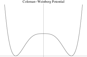
Figure 2: Coleman Weinberg potential for the SC field $\phi$ (See Eq. 3), at zero temperature.

As our starting point, the SuperCool (SC) field $\phi$ has a Coleman Weinberg (CW) potential (See Fig. 3) at zero temperature. Furthermore, SC field is a complex scalar, which is charged under a U(1)_X Abelian group. We have enforced classical scale invariance on the potential ( known as the “no bare mass” condition) such that

$$\frac{d^{2}\text{V}(\phi)}{d\phi^{2}}\bigg{|}_{\phi=0}=0.$$ (2)

Classically, the SC field is simply of the form $\lambda\phi^{4}$ and is scale invariant. Quantum corrections modify the classical potential breaking the scale invariance. Then, dimensional transmutation generates a nonzero vacuum expectation value $\langle\phi\rangle$ i.e. vev. At one loop, the potential Coleman:1973jx is

$$\text{V}(\phi)=\frac{3g_{X}^{4}}{32\pi^{2}}|\phi|^{4}\bigg{(}\ln\bigg{(}\frac{|\phi|}{\langle|\phi|\rangle}\bigg{)}-\frac{1}{4}\bigg{)}+\Lambda^{4}$$ (3)

where $g_{X}=0.4$ is the charge of the scalar field. $\Lambda$ is the usual cosmological tuning, which will generate the vacuum energy during inflation V$(0)=\Lambda^{4}$ and sets the true vacuum to zero V$(\langle\phi\rangle)=0$. We will take $\Lambda\simeq 1$ TeV and $\langle|\phi|\rangle\simeq 10$ TeV to be concrete. Clearly, the vev $\langle\phi\rangle$ and the scale of inflation are connected for a given $g_{X}$. The scale of inflation i.e. $\Lambda$ can be larger or smaller than 1 TeV; we will comment later. So far, we have neglected temperature effects.

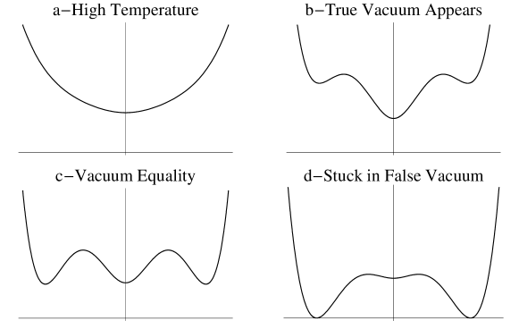
Figure 3: The effective potential at different temperatures: a–At high temperatures, only one vacuum state exist. b–Eventually, other vacuum states appear. c–At the transition temperature, the Universe will be in the symmetric minima. d–As the temperature drops, the symmetric vacuum remains metastable.

II.1 Stabilized Potential

At a nonzero temperature, finite temperature effects stabilize the false vacuum of the SC potential. Near the origin of $\phi$, we can approximate the finite temperature part of the effective potential with

$$V(\text{T},\phi)=\mathcal{O}(1)\text{T}^{4}+(1/8)\,\text{T}^{2}\,\phi^{2}+\mathcal{O}(\phi^{4})$$ (4)

(Witten:1980ez ; Dolan:1973qd ; Weinberg:1974hy ). At very high temperatures (Fig.3-a), the symmetric minimum is the only vacuum state and the Universe sits at $\phi=0$. As the temperature of the Universe drops (Fig.3-b), the true vacuum appears near $\phi=\langle\phi\rangle$. The potential evolves only gradually from high temperatures. As the Universe continues to cool reaching the transition temperature (Fig.3-c), the Universe will still be in the symmetric minima Guth:1980zk ; Witten:1980ez . At temperatures below the transition temperature (Fig.3-d), thermal tunneling can allow the field to transition to the true vacuum, but the rate is exponentially small. We will follow an argument first given by Witten Witten:1980ez .

The tunneling rate $\Gamma$ will be dominated by the O(3) thermal instanton S₃ Linde:1981zj . We have also considered an O(4) instanton Linde:1981zj and a Hawking-Moss instanton Hawking:1981fz , which are subdominant.

$$\Gamma\sim\text{T}^{4}\bigg{(}\frac{\text{S}_{3}(\text{T},\phi)}{2\pi\,\text{T}}\bigg{)}^{3/2}\exp[{-\frac{\text{S}_{3}}{\text{T}}}]$$ (5)

where T is the temperature of the Universe. Near the origin and the barrier (the part of the potential relevant for tunneling), we can transform Eq. 3 with a trick invented by Witten Witten:1980ez

$$\text{V}(\text{T},\phi)=\frac{\text{T}^{2}}{8}|\phi|^{2}-\frac{3g_{X}^{4}}{32\pi^{4}}|\phi|^{4}\bigg{(}\ln\bigg{(}\frac{\text{M}_{X}}{\text{T}}\bigg{)}+\mathcal{O}(1)\bigg{)}$$ (6)

where M${}_{X}=g_{X}\langle\phi\rangle$ is the mass of the U(1)_X gauge boson. With Eq. 3 now in the form of Eq. 6, we have an exact solution of the O(3) instanton.

$$\text{S}_{3}=\frac{4\pi^{2}}{3}\frac{\text{T}}{g_{X}^{3}\ln(\text{M}_{X}/\text{T})}19$$ (7)

where the factor of 19 is a geometric factor.

In SCI, the Universe is stable against tunneling to the true vacuum. At most, only some small part of the Universe can transition to the true vacuum. Guth and Weinberg Guth:1982pn have shown that the tunneling rate (per unit time per unit volume) $\Gamma$ compared to the Hubble 4-Volume

$$\beta=\Gamma/\text{H}^{4}\mathrel{\raise 1.29167pt\hbox{$>$\kern-7.5pt\lower 4.30554pt\hbox{$\sim$}}}9/4\pi=\beta_{c},$$ (8)

must be larger than $\beta_{c}$ for the Universe to transition from the false to the true vacuum. We show that $\beta$ for the SC field is much smaller than $\beta_{c}$ during inflation. Hence, the Universe is stuck in the false vacuum state. Rapid tunneling to the true vacuum can only occur when S${}_{3}\rightarrow 0$. Upon inspection, only as $g_{X}$ becomes large or T goes to zero does S${}_{3}\rightarrow 0$, but we show that in either case tunneling will still be extremely small. Hence, a new mechanism will be needed to generate a graceful exit.

First, $g_{X}$ never becomes large and stays perturbatively small as the temperature drops from the TeV scale down to a fraction of an electron volt (T$\leq 10^{-2}$eV). At which point in the next section, we show that the Witten mechanism can generate a graceful exit. More generally if the SC field was charged under a non-Abelian gauge group, we would need to be more careful (See PhysRevD.24.1699 ).

Second as the temperature drops, the logarithm $\ln(\text{T}/\text{M}_{X})$ in Eq. 7 blows up. Regardless $\beta$ (for the inflaton potential) is much less than $\beta_{c}$ during inflation, since the pre-factor in Eq. 5 (which scales like T⁴) goes to zero sufficiently fast to counteract the Log factor in the exponential. Furthermore, $\beta$ is sufficiently small to avoid constraints from BBN and CMB Turner:1992tz .

In addition, a technical concern could lead to a much larger tunneling rate. At the origin of the SC potential, the one loop perturbative calculation given in Eq. 3 becomes no perturbative. In principle, the actual potential could be very different leading to a much larger tunneling rate. The worry is unfounded. Subsequently, a non-perturbative calculation 1997MPLA…12.2287L has been preformed which verifies that Eq. 3 is still correct. Hence, the Universe is safe from transitioning from the false vacuum to the true vacuum during inflation. In fact, the Universe never tunnels for even arbitrarily low temperatures. For inflation to end, we will need to introduce new physics.

II.2 Ending Inflation (Witten Mechanism):

Witten’s mechanism generates a graceful exit and ends inflation. We implement the Witten mechanism by introducing a set of QCD like fermions charged under a non-Abelian gauge group with a Yukawa coupling to the SC field V${}_{\text{y}}(\phi)=\sum y_{i}\phi\ast(q_{R}\bar{q}_{L})_{i}+$ h.c. where $y_{i}$ is the Yukawa coupling for respectively the right and left-handed fermions $q_{R}$ and $q_{L}$. The SC field $\phi$ is a singlet under the non-Abelian gauge group. Only some of the right handed quarks and left handed quarks are charged under the U(1)_X such that the Yukawa terms are gauge invariant. We also must be careful how we assign U(1)_X charges to the quark like fermions to ensure that the theory is anomaly free. As with QCD, we can pick a sufficiently small coupling constant such that the theory will only become strongly coupled at a low scale. Finally, the fermion loop corrections have not been included in Eq. 3. Qualitatively the evolution of the aulos field remains unchanged unless there are a large number of fermions with large Yukawa couplings.

When the temperature of the Universe drops below the strong coupling scale $\Lambda_{S}$ of the non-Abelian gauge group, the vacuum of the non-Abelian gauge group freezes, and the fermions gain a vev

$$\text{V}_{y}(\phi)\rightarrow\bigg{(}\sum y_{i}\langle q_{R}\bar{q}_{L}\rangle_{i}\bigg{)}\ast\phi+\text{h.c.}=\epsilon\ast\phi+\text{h.c.}.$$ (9)

The vacuum seizes, which dynamically breaks any global symmetries possessed by the quark like fermions $q_{R}q_{L}$, and the U(1)_X gauge symmetry. If some of the $y_{i}\simeq 1$, then $\epsilon\simeq\Lambda_{S}^{3}\simeq\text{T}_{c}^{3}$, where T_c is the temperature at which the vacuum of non-Abelian gauge group freezes. As we show below, the barrier trapping the SC field in the false vacuum goes away once the non-Abelian gauge group freezes.

Concrete Example

We now work through a concrete case of SCI with $\Lambda\simeq 1$TeV and $\langle|\phi|\rangle\simeq 10$ TeV. Initially, the Universe is radiation dominated. The Universe then cools and becomes stuck in the false vacuum. The energy density of Universe becomes dominated by vacuum energy. The Universe begins superluminal expansion once the temperature falls below a few hundred GeV (N.B. The precise temperature when superluminal growth begins depends upon the number of relativistic degrees of freedom. At temperatures between 100GeV to 1 TeV, there are $\mathcal{O}(100)$ relativistic degrees of freedom from the standard model. In which case, superluminal expansion begins once the temperature falls to $\sim 300$ GeV). As a conservative estimate, we will assume that inflation really only starts once the temperature of the Universe is a 100 GeV. Inflation must last for at least 30 efolds to solve the horizon and flatness problems (See Eq. 16). After 30 efolds, the temperature of the Universe drops to $\sim 10^{-2}$ eV and the non-Abelian gauge group freezes. See Eq. 9.

Once the non-Abelian gauge group freezes, the barrier goes away. Near the origin, Eq.6 together with Eq.9 has the form

$$(\epsilon\phi+\text{h.c.})+\frac{1}{2}\,\tilde{m}^{2}|\phi|^{2}-\frac{1}{4}\,\tilde{\lambda}|\phi|^{4}$$ (10)

(See Fig. 1). We note that the linear term will destabilize the meta-stable vacuum state ($\phi\simeq 0$ ) by eliminating the barrier if

$$|\epsilon|\geq\frac{2}{3^{3/2}}\frac{\tilde{m}^{3}}{\tilde{\lambda}^{1/2}}.$$ (11)

Upon substituting in values for $\epsilon$, $\tilde{m}$, and $\tilde{\lambda}$, we see that as the temperature drops so does m; while, $\tilde{\lambda}$ increases. In Fig.1, the barrier trapping the inflaton at the origin goes away once T $\simeq$ T${}_{c}\sim 10^{-2}$ eV, with $g_{X}=0.4$, M${}_{\chi}\simeq$ 4 TeV and T${}_{c}\simeq\Lambda_{S}\simeq 10^{-2}$ eV. In sum, the Universe goes through 30 efolds of inflation solving the flatness and horizon problems, the barrier goes away, and the SC field goes rapidly to the true vacuum. The Universe then reheats as discussed below.

II.3 Reheating

Once the barrier goes away, the field quickly goes to the true minimum, where it may oscillate and decay into standard model particles. Reheating can be virtually instantaneous for the decay rate $\Gamma_{\phi}\gg$H. We might have a complicated decay process into standard model particles. For instance, the SC field might decay into particles charged under U(1)_X which subsequently decay into standard model particles. If the inflaton only partially decays into standard model particles, then the SC sector might be related to dark matter. We will instead treat the case where $\phi$ decays only into standard model particles and in particular Z bosons. The choice is idiosyncratic; many other reasonable decay routes exist (for instance, the SC field could decay into Higgs bosons).

In general, there are only 3 couplings between a hidden sector and the standard model which are renormalizable and gauge invariant: a vector coupling to hypercharge $B_{\mu\nu}$ (kinetic mixing), a scalar coupling to the Higgs HH^† , and a spinor coupling with a Higgs-neutrino operator HL 2009arXiv0909.4541W . We will focus on the kinetic mixing Holdom:1985ag between hypercharge $B_{\mu\nu}$ and the U(1)_X SC gauge boson $X_{\mu\nu}$. We have, thus, expanded the standard model $\rightarrow$ SU(3)$\times$SU(2)${}_{\text{L}}\times$U(1)${}_{Y}\times$U(1)_X. In which case, the standard model will contribute to the CW potential Eq. 3. If the EW phase transition occurs during inflation, then there will be a threshold correction to the CW potential. The renormalization condition Eq. 2 can be maintained by matching the renormalization group flow equations as it runs from the IR up to the threshold and from the UV down to the threshold. The IR and UV are then necessarily sensitive to each other, which only highlights the mysterious nature of the “no bare mass” condition.

In the case of kinetic mixing between hypercharge U(1)_Y $B^{\mu\nu}$ and the X boson U(1)_X $X^{\mu\nu}$, the kinetic energy terms go like

$$\mathcal{L}_{\text{KE}}^{BX}=-\frac{1}{4}B_{\mu\nu}B^{\mu\nu}-\frac{1}{4}X_{\mu\nu}X^{\mu\nu}+\frac{\chi}{2}B_{\mu\nu}X^{\mu\nu}$$ (12)

where $\chi$ (at an effective level) is an arbitrary mixing parameter and can take any value (which is how we treat $\chi$ for the remainder of the paper). N.B.  in some top down approaches the parameter $\chi$ can arise from integrating out vector like fermions charged under both the hidden U(1)_X and hypercharge Holdom:1985ag , which gives $\chi\sim 10^{-2}$.

Upon diagonalizing the kinetic term Eq. 12 with a GL(2,R) rotation and then diagonalizing the gauge boson mass matrix with an O(3) rotation, we can write $X_{\mu}$ in terms of the mass eigenstates of the standard model Z boson and a Z^′ 2009arXiv0909.4541W . We now have the coupling of the SC field $\phi$ to the Z boson.

We can, then, determine the decay rate of the SC field into Z bosons. When the mass of the U(1)_X gauge boson M_X is large compared to the unmixed Z boson mass M${}_{Z_{0}}$ (the $0$ refers to the field before mixing) or $\chi$ is small, the decay rate of the SC inflaton into a pair of Z bosons (Lee:1977yc ,  Lee:1977eg , and Gunion:1989we ) is then

$$\Gamma_{\phi\rightarrow\text{ZZ}}=\frac{\pi}{6}M_{\phi}(g_{X}\,\sin\theta_{w}\eta\Delta z)^{4}\frac{\sqrt{1-x}}{x^{2}}(3x^{2}-4x+4)$$ (13)

where M_ϕ ($\sim 300$ GeV) is the mass of the SC inflaton, $\sin\theta_{w}$ is the Weinberg angle, $\Delta z=(M_{Z_{0}}/M_{X})^{2}$, $x=4M_{Z}^{2}/M_{\phi}^{2}$, $\eta=\chi/\sqrt{1-\chi^{2}}$ and $g_{X}=0.4$. We find that $\Gamma_{\phi\rightarrow\text{ZZ}}=0.03$ eV$\gg$ H $\simeq 10^{-4}$ eV, where we have taken $\chi=.9$ and $M_{Z^{\prime}}\simeq M_{X}$ ($\sim 4$ TeV). The field will predominantly decay into Z bosons, if the masses of all other particles which couple to $\phi$ are more massive than $M_{\phi}$. For instance the QCD like fermions have Yukawa couplings which are $\mathcal{O}$(1) and have a mass $\sim$10 TeV.

We have assumed a large mixing $\chi$ between the $Z_{0}$ and $X$ boson but the large difference in the masses suppresses the decay rate. One could imagine a slightly less massive X particle which would lead to a much larger decay rate. Regardless, the Universe rapidly reheats converting the vacuum energy into radiation. With 100 relativistic degrees of freedom, the Universe then reheats to a temperature $\simeq 500$ GeV, which is sufficiently high to do EW baryogenesis Wainwright:2009mq . If we had a smaller mixing parameter, we could then have a smaller decay constant and a lower reheat temperature.

The SC field can avoid collider constraints. The Z^′ is heavy enough to avoid present collider bounds 2011PhRvD..83g5012A ; Appelquist:2002mw . The coupling of $\phi$ to the standard model is strongly suppressed in this case due to large mass ratio of Z to Z^′. Hence, the toy model is consistent with collider bounds. In a future paper, we will consider collider searches for the SC inflaton doug1 .

II.4 Scale of Inflation

Cosmological considerations can place an upper and lower limit on the scale of SCI. On the low end, any inflation model must satisfy Big Bang Nucleosynthesis (BBN) constraints. In which case, the Universe then reheats to at least a few MeV. Baryogenesis could potentially, also, place constraints on the minimal scale of inflation. If the scale of inflation and reheat temperature is above 100 GeV, then one can use EW baryogenesis or leptogenesis to generate a baryon asymmetry Wainwright:2009mq . At present, we know of no published models of baryogenesis which work with the scale of inflation below 100 GeV. Thus, our present lack of imagination with regards to baryogenesis will require that inflation occurs above 100 GeV.

An aulos field might get around the above argument. As defined in the introduction, an aulos field is any field which has a small mass during inflation and a large mass at the end of inflation. Later in the paper, we will use the aulos mechanism to generate density perturbations. In a different direction, the aulos mechanism in conjunction with the Affleck-Dine Mechanism (ADM) Affleck:1984fy could also be used to generate a baryon asymmetry even if the scale of inflation is below 100 GeV. We would like to emphasize that the field generating a baryon asymmetry and the field generating density perturbations are not necessarily one and the same.

The Affleck-Dine Mechanism (ADM) can occur with a reheat temperature as low as a few MeV, but ADM without the aulos mechanism requires that the scale of inflation be above $10^{9}$ GeV Dine:2003ax ; Banks:1996ea . The constraint on the scale of inflation from ADM follows from 2 requirements: 1– the mass of the field carrying baryon number must be larger than the mass of the proton when the field decays. 2– the field must also be Hubble-damped during inflation.

An aulos field carrying baryon number can satisfy the 2 ADM requirements and could be used to do baryogenesis at a scale of inflation below $10^{9}$ GeV. The mass of the aulos field is small during inflation so the field is Hubble damped satisfying the first requirement regardless of the inflationary scale. At the end of inflation, the mass of the field becomes large satisfying the second requirement. The field begins to oscillate and generate baryon number via ADM. In principle, one can have baryogenesis for a very low inflationary scale (potentially MeV scale). We will leave detailed model building for a future paper doug1 . Regardless from observational constraints, the scale of inflation must still be larger than a few MeV.

On the other end of the scale, SCI most naturally occurs for $\Lambda\lesssim 100$ TeV due to the appearance of non-renormalizable terms and the number of efolds necessary to solve the horizon and flatness problems. For instance, we have so far neglected a term which arises in general relativity

$$-\frac{1}{2}\xi R|\phi|^{2},$$ (14)

where $R=-32\pi G\Lambda^{4}$. $G$ is Newton’s constant and $\Lambda^{4}$ is the vacuum energy during inflation. $\xi$ characterizes the coupling of the SC field $\phi$ to gravity. In the minimally coupled case ($\xi=0$), there is no constraint on the scale of inflation. The scale can be arbitrarily large. As another example, if the “no bare mass” hypothesis is true, then it is sensible to believe that the SC field is classically conformally invariant which implies that $\xi=1/6$ Callan:1970ze  Abbott:1981rg . We note that if we include loop corrections $\xi$ is a renormalizable coupling constant that runs to a fix point $\xi=1/6$ in the IR but can have a negative value in the UV Hill199221 .

Regardless, Eq. 14 can be problematic. If $\xi>0$, Eq. 14 stabilizes the false vacuum, in which case inflation could never end. If $\xi<0$, Eq. 14 could destabilize the false vacuum state, in which case inflation could end too soon. Hence, we require that inflation ends before Eq. 14 becomes important

$$\text{T}_{c}^{2}\gtrsim|\xi R|\propto|\xi|G\Lambda^{4}$$ (15)

where T_c is the critical temperature when inflation ends (See Eq. 11).

The number of efolds of inflation necessary to account for the horizon problem goes like 1990eaun.book…..K

$$\text{N}_{min}=30+\frac{1}{3}\left(2\log\left[\frac{\Lambda}{1\text{ TeV}}\right]+\log\left[\frac{\text{T}_{RH}}{1\text{ TeV}}\right]-\log\left[\gamma\right]\right)$$ (16)

where $\Lambda$ is the scale of inflation, T_RH is the reheat temperature at the end of inflation, and $\gamma$ is the amount of any subsequent entropy production after inflation and reheating. Also, the number of efolds necessary to resolve the flatness problem is similar to the number of efolds necessary to solve the horizon problem (See 1990eaun.book…..K Chapter on inflation). We will require that the number of efolds of inflation be greater than or equal to Eq. 16.

Tension between Eq. 15 and Eq. 16 places an upper limit on the scale of SCI. The necessary number of efolds increases with the scale of inflation (first term of Eq. 16), but Eq. 15 pushes up T_c with an increasing scale of inflation. We can only satisfy both Eq. 15 and Eq. 16 if $\Lambda\lesssim 100$ TeV for $\xi\sim\mathcal{O}(1)$.

SCI comfortably occurs between 100 TeV and 100 GeV (also potentially even the MeV scale), but inflation at the TeV scale would certainly be interesting. In many models beyond the standard model, new machinery at the TeV scale is introduced to explain EW symmetry breaking: gauge mediation, little Higgs models, large extra dimensions etc.. Theoretically, it is compelling to connect inflation to the dynamics which drive EW symmetry breaking. Second, LHC and future colliders can effectively probe the TeV scale. Inflation could become a laboratory science. At the moment, we can only probe inflation indirectly through cosmology. Finally, the low scale of inflation inherently avoids many pitfalls of high scale inflation such as overclosure from gravitinos to moduli and trans-Planckian physics.

III No Eternal Inflation

Virtually, all known models of inflation suffer from eternal inflation such as chaotic inflation 1986PhLB..175..395L and new inflation (See Fig. 4). There are a few exceptions such as Baumann:2007np which require a large amount of fine-tuning. More generally as noted by Guth, most rolling models without eternal inflation are pretty contrived from a field theoretical perspective Guth:2000ka .

As a simple example of eternal inflation consider chaotic inflation, which occurs at large field values. A scalar field is displaced from the true minimum. The potential of the scalar field V$(\phi)$ is sufficiently flat such that the field rolls very slowly to the true vacuum state. As the Universe rolls down, quantum fluctuations of the field can cause a small patch of the Universe to go up the potential, which cause the fluctuation to grow (See Fig. 4). A small patch can continue to fluctuate up the potential until the quantum fluctuations of the field become order one i.e. $\Delta\rho/\rho\sim 1$, at which point the patch can no longer roll back down. The patch begins to exponentially expand. At which point, the Universe begins to inflate eternally and only an exponentially small fraction of the Universe is not eternally inflating (See Guth:2000ka for an introduction to eternal inflation). These small pocket Universes could evolve into a Universe which looks like ours or could be very different.

If we had a full picture of the eternally inflating Universe or Multiverse for short, we could generate a probability distribution for the properties of different pocket Universes, such as the cosmological constant, the amount of dark matter in the Universe etc.. Then in fact, eternal inflation could be able to make various predictions and be tested.

Sadly, counting in an infinite Universe proves difficult. To quote Alan Guth, “In an eternally inflating Universe, anything that can happen will happen; in fact, it will happen an infinite number of times. Thus, the question of what is possible becomes trivial – anything is possible, unless it violates some absolute conservation law. To extract predictions from the theory, we must therefore learn to distinguish the probable from the improbable.” Guth:2000ka . Hence at worst, we have given up any predictive power of inflation since anything and everything is possible, but if one had a good way to count the relative occurrence of different pocket Universes, we could regain the predictive power of inflation.

At present, there is no agreed method of determining the relative probability of different pocket Universes, or in other words we have no sensible measure of the Multiverse. In fact, eternal inflation and various measures so devised have instead led to a series of problems such as the youngness problem, Boltzmann brains, etc., or make predictions which are wholly counterintuitive. For instance, the geometric or light cone measure (introduced by Bousso Bousso:2006ev ) predicts that time itself will end in the next 5 Billion years Bousso:2010yn . (See Freivogel:2011eg for a recent review). One might be interested in coming up with an inflationary model which avoids eternal inflation in the first place.

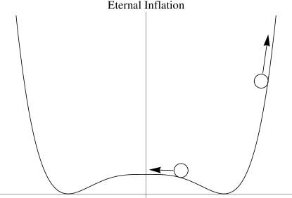
Figure 4: Eternal inflation occurs at the origin of slowly rolling fields (as in new inflation) and at large field values (as with chaotic inflation). Quantum fluctuations prevent the field from rolling to the true vacuum as represented with the arrows.

Eternal inflation occurs when

$$\frac{\delta\rho}{\rho}\mathrel{\raise 1.29167pt\hbox{$>$\kern-7.5pt\lower 4.30554pt\hbox{$\sim$}}}1\rightarrow\frac{V(\phi)^{3/2}}{m_{pl}^{3}}\mathrel{\raise 1.29167pt\hbox{$>$\kern-7.5pt\lower 4.30554pt\hbox{$\sim$}}}|V^{\prime}(\phi)|$$ (17)

where $m_{pl}=2.4\times 10^{18}$ GeV is the reduced Planck mass, $V(\phi)$ is the SC field but more generally is any scalar potential. The prime refers to partial differentiation with respect to $\phi$. For any scalar field, there are potentially two problematic field values. First in the large field case ($\phi\rightarrow\infty$), the field could undergo chaotic eternal inflation as discussed above. Second near the hilltop of the potential (a local maximum– $V^{\prime}(\phi)=0$), a scalar field can also undergo eternal inflation as with the original new inflation models.

Regardless, SCI actually avoids eternal inflation. We consider both the hilltop and the chaotic cases. In the hilltop case ($V^{\prime}(\phi)=0$), we show in the Appendix, that if

$$\sqrt{|V^{\prime\prime}(\phi)|}>3\text{H},$$ (18)

then there is no eternal inflation. Conversely if 3H$>\sqrt{|V^{\prime\prime}(\phi)|}$, then there will be eternal inflation. There is a hilltop point near the origin of the SC field ($\phi\simeq 0$). We note that the tadpole term shifts the hilltop point away from the origin. By plugging in numbers, it is clear that there is no eternal inflation near the origin since slow roll is violated.

SCI can avoid chaotic or large field value eternal inflation. In the large field case for the SC potential Eq. 3, we violate Eq. 17 once $\phi>m_{pl}$. We have so far not discussed the non-renormalizable terms given in Eq.1. The SC potential $V(\phi)$ reaches a maximum before $\phi>m_{pl}$ by including a non-renormalizable term.

Non-renormalizable terms are a necessary component of an effective field theory. For instance, a field which is non-minimally coupled to gravity has just such a term. Non-minimal coupling was discussed in the previous section. More generally, non-renormalizable terms can arise, when embedding a effective field theory in a more fundamental theory. Non-renormalizable terms will go like $(\pm)\lambda_{n}\Lambda_{c}^{-n}\phi^{4+n}$, where $\Lambda_{c}$ is the ultra-violet cut off and $\lambda_{n}$ is positive. We now include a non-renormalizable term in the potential of the SC field Eq. 3

$$V(\phi)=\frac{\lambda}{4}|\phi|^{4}\bigg{(}\ln\bigg{(}\frac{|\phi|}{\langle\phi\rangle}\bigg{)}-\frac{1}{4}\bigg{)}-\frac{\lambda_{2n}}{2n+4}\frac{|\phi|^{2n+4}}{\Lambda_{c}^{2n}}$$ (19)

where $\lambda=3g_{X}^{4}/8\pi^{2}$ (See Fig. 5). For simplicity, we have neglected the cosmological tuning parameter in Eq. 3 (N.B. neglecting $\Lambda\ll\Lambda_{c}$ will not alter our results ) and the tadpole term which is irrelevant at large field values. By inspection of Eq. 19, there exists a hilltop point $\phi_{0}$ where $V(\phi_{0})$ is a maximum of the potential.

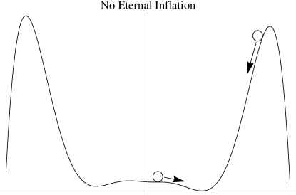
Figure 5: We have added a non-renomalizable term to the SC potential Eq. 3. Hence, the potential has no chaotic eternal inflation. In addition, the potential does not have eternal inflation at the hilltops since the field does not slow roll at the hilltop points.

SCI also avoids eternal inflation at the hilltop point $\phi_{0}$. Near $\phi_{0}$ we can approximate Eq. 19 with

$$V(\phi)=\frac{\lambda^{\prime}}{4}|\phi|^{4}-\frac{\lambda_{2n}}{2n+4}\frac{|\phi|^{2n+4}}{\Lambda_{c}^{2n}}$$ (20)

where $\lambda^{\prime}=\lambda\ln(\Lambda_{c}/\langle\phi\rangle)$ when $4n^{2}\ln(\Lambda_{c}/\langle\phi\rangle)>\ln(\lambda/\lambda_{2n})$ and $\ln(\Lambda_{c}/\langle\phi\rangle)>1/4$. Then using Eq. 18, SCI will not have eternal inflation at $\phi_{0}$ if

$$\frac{|\phi_{0}|}{\sqrt{2n+4}}<\frac{2}{3}m_{pl}\,\,\,\,\,\,\text{with}\,\,\,\,\,\,|\phi_{0}|=\bigg{(}\frac{\lambda^{\prime}}{\lambda_{2n}}\bigg{)}^{\frac{1}{2n}}\Lambda_{c},$$ (21)

where $m_{pl}$ is the reduced Planck mass. As an example, consider a dimension 6 operator and assume the cut off is the reduced Planck mass. The non-renormalizable term is then equivalent to Eq. 14 i.e. a non-minimal coupling to gravity. We then find that there will be no eternal inflation for $\lambda_{2}>3/8\lambda^{\prime}\simeq 10^{-2}$ or equivalent in terms of Eq. 14 that $\xi<-0.1$. Also, we have avoided chaotic inflation since $|\phi_{0}|<m_{pl}$. Hence, SCI can avoid eternal inflation by introducing non-renormalizable terms or by simply coupling the SC field to gravity.

In fact, the above scenario is quite general. $\xi$ is generally not constant and runs with the energy scale of the relevant interactions. Hill & Salopek Hill199221 calculated the RGE of $\xi$ for a composite scalar field but they note that their conclusion holds for an arbitrary scalar field as well. They found that $\xi=1/6$ is an IR fixed point. In the UV (or at large field values), $\xi$ can easily become large and negative, which naturally circumvents eternal inflation from happening as shown above.

In many ways it is not surprising that SCI avoids eternal inflation. Inflation driven by a rolling field requires an unusual situation with the necessity of having an incredibly flat potential. After one has gone to the trouble of having an incredibly flat potential in the first place, then eternal inflation can occur. SCI does not depend upon slow roll dynamics and avoids eternal inflation.

IV Density Perturbations

The presence of a thermal bath (which is necessary in SuperCool (SC) inflation) will strongly suppress curvature perturbations. Adiabatic density perturbations go like

$$\xi=\frac{\delta\rho}{\rho+p}$$ (22)

where $\delta\rho$ is the variation of density and $\rho$ and $p$ are respectively the average energy density of the Universe and pressure at the time a perturbation leaves the horizon. For a discussion on perturbations, see 1990eaun.book…..K and references there in i.e. Bardeen:1983qw .

As with slow roll inflation, one might imagine introducing a single slowly rolling scalar field $\phi_{r}$ to generate density perturbations. In this case, $\delta\rho\sim$ H V${}^{\prime}(\phi_{r})$ where H is the Hubble parameter when the perturbation leaves the horizon. V($\phi_{r}$) is the potential of the scalar field. In slow roll, V${}^{\prime}(\phi_{r})=-3$H$\dot{\phi}_{r}$. The prime refers to partial differential with respect to $\phi_{r}$, and the dot refers to differentiation with respect to time. $\rho+p$ is summed over all matter and energy components. Typically for inflation, $\rho+p=\dot{\phi}_{r}^{2}$, but if there is a thermal background then we must include thermal radiation and pressure where $\rho_{r}=1/3p_{r}$. The thermal component will dominate the sum $\rho+p$, which will suppress adiabatic perturbations generated by the rolling field.

One might imagine that thermal variations might generate perturbations, but the thermal variation across the initial patch is exponentially small. Equilibrium processes wash out any temperature variations across the patch ($\delta\rho_{r}/\rho+p\ll 1$), unless there is a process to generate perturbations on all scales in the plasma just prior to the start of inflation. We will not consider this case any further, but will leave the problem for a separate paper doug1 . Instead, we will turn to the aulos mechanism as discussed in the introduction.

IV.1 Aulos Mechanism

We introduce an explicit model to implement the aulos mechanism as outlined in the introduction. We introduce a new complex scalar field $\chi_{a}$ and 2 new scalar fields $\chi_{b}$ and $\chi_{c}$. The new fields have a potential

$$V_{abc}=-\frac{\mu^{2}}{2}(\chi_{b}^{2}+\chi_{c}^{2})+\frac{\lambda}{4}(\chi_{b}^{2}+\chi_{c}^{2})^{2}$$ (23)

$$+\frac{\lambda_{\chi}}{4}|\chi_{a}|^{4}\bigg{(}\ln\bigg{(}\frac{|\chi_{a}|}{\nu}\bigg{)}-\frac{1}{4}\bigg{)}+\sum_{i}^{abc}\bigg{(}\frac{\alpha_{i}\text{T}^{2}}{2}|\chi_{i}|^{2}\bigg{)}$$

$$+\frac{\lambda_{b}}{2}\bigg{(}\chi_{b}^{2}-\chi_{c}^{2}\bigg{)}|\chi_{a}|^{2}-\frac{\lambda_{a\phi}}{2}|\phi|^{2}|\chi_{a}|^{2}.$$

All of the coefficients are positive. There is an O(2) symmetry between $\chi_{b}$ and $\chi_{c}$, which is broken by the interaction term with $\chi_{a}$. $\chi_{a}$ has a U(1)_a axial symmetry. $\chi_{b}$ and $\chi_{c}$ get a vev when ($\mu>\alpha_{b}$T² & $\mu>\alpha_{c}$T²). ).

We require that $\chi_{a}$ is independent of temperature. If the field is temperature dependent then it will be difficult to generate the necessary density perturbations for inflation. We could argue that $\chi_{a}$ has a zero temperature during inflation. Instead, we cancel the temperature dependent term of $\chi_{a}$ in Eq. 23 ($\alpha_{a}$T${}^{2}|\chi_{a}|^{2}$) by setting

$$\alpha_{a}=\frac{\lambda_{b}}{\lambda}(\alpha_{c}-\alpha_{b}),$$ (24)

which requires a careful selection of the matter coupled to $\chi_{a}$, $\chi_{b}$, and $\chi_{c}$ given ($\lambda_{b}/\lambda$). The coefficients $\alpha_{i}$ in Eq. 23 depends upon the matter content coupled to $\chi_{i}$. We will require that $\chi_{b}$ and $\chi_{c}$ have different couplings to fermions i.e. $\alpha_{c}\neq\alpha_{b}$. The different couplings to matter will then break the O(2) symmetry of Eq. 23 and potentially induce a different $\lambda$ for $\chi_{b}$ and $\chi_{c}$ due to quantum corrections. One can insure that $\chi_{b}$ and $\chi_{c}$ do have the same $\lambda$ by again carefully choosing the matter content which couples to $\chi_{b}$ and$\chi_{c}$ such that the loop corrections will be the same for $\chi_{b}$ and $\chi_{c}$. In addition, we will require that $\lambda_{b}/\lambda$ is a rational number to allow for the cancellation of ($\alpha_{a}$T${}^{2}|\chi_{a}|^{2}$). This will require a fair amount of model building. In a more fundamental theory one might be able to find such a scenario. Otherwise naively, Eq. 24 requires severe tuning. We do not address the naturalness of such a scenario at this time.

Regardless, the interaction term, now, cancels the $\alpha_{a}$T${}^{2}\chi_{a}^{2}$ term; $\chi_{a}$ has a Coleman Weinberg potential and then undergoes dimensional transmutation which spontaneously breaks U(1)_a i.e. ($\chi_{a}$ acquires a vev $\nu$). With the vev of $\chi_{a}$ ($\nu\neq 0$), we redefine $\chi_{a}$ in terms of a radial field ($\sigma$) and an angular field ($a$) which corresponds to the pseudo Nambu-Goldstone boson of $\chi_{a}=(\nu+\sigma)e^{ia/\nu}$. We will associate the pseudo Nambu-Goldstone boson ($a$) with the aulos field. As one final note, we can avoid eternal inflation in the aulos sector in much the same way that we avoided eternal inflation in the inflaton sector.

IV.2 Aulos Mass

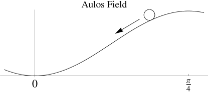
Figure 6: Aulos potential Eq. 25 in units of $\nu$. During inflation, the aulos vev and mass are small. At the end of inflation, the vev and mass become large.

We introduce a mass term for the aulos field ($a$), by softly breaking the U(1)_a symmetry. The potential of the aulos field is then,

$$V(\chi_{a})_{S} =\frac{\lambda_{s}}{4}((\chi_{a})^{4}+(\chi_{a}^{\star})^{4})$$ (25)

$$=\frac{\lambda_{s}(\nu+\sigma)^{4}}{2}\bigg{(}\cos\bigg{(}\frac{4a}{\nu}+\pi\bigg{)}+1\bigg{)}$$

where $\lambda_{s}$ is a dimensionless parameter which gives the size of the symmetry breaking and $\chi_{a}^{\star}$ is the complex conjugate of $\chi_{a}$. A soft breaking term such as Eq. 25 can arise from a constrained instanton first introduced by t’Hooft PhysRevD.14.3432 and more fully developed by Affleck Affleck:1980mp . We will leave a more careful analysis for the future and treat Eq. 25 at an effective level. In Eq. 25, we have shifted the aulos field such that the minimum of the potential is given when $4a/\nu\rightarrow 0$ (See Fig. 6). We might worry about the formation of domain walls. With the given breaking term there are 4 degenerate vacua. But the worry is unfounded. $\chi_{a}$ and the aulos field never reheat at the end of inflation. In which case, the Kibble mechanism will not generate domain walls.

Expanding the cosine at the minimum gives that

$$m_{a}^{2}=16\lambda_{s}\nu^{2}=128\lambda_{s}f_{a}^{2}$$ (26)

where $m_{a}$ is the mass of the aulos field and $f_{a}=\nu/4$ is the decay constant for the aulos field. The mass is proportionate to the spontaneous symmetry breaking scale. Hence, the mass will vary if the spontaneously symmetry breaking scale changes.

IV.3 Aulos Evolution

In our toy model during inflation, the aulos field is Hubble damped with 3H $\simeq 10^{-3}$ eV $\geq m_{a}$. The vev of the SC field is zero and does not contribute to the vev of $\chi_{a}$. The vev of $\chi_{a}$ is initially small. At the end of inflation, the SC field gets a large vev $\langle\phi\rangle$ which will generate a large and negative effective mass term for $\chi_{a}$. Then from Eq. 23, $\chi_{a}$ gets a new large vev ($\nu$)

$$\nu^{2}\rightarrow\frac{\lambda_{a\phi}\langle\phi\rangle^{2}}{\lambda_{\chi}}.$$ (27)

The aulos mass and decay constant become large. See Eq. 26.

When $m_{a}\geq$3H, the aulos field begins to oscillate and generates a condensate with an energy density

$$\rho_{a}=\frac{1}{3}m_{a}^{2}f_{a}^{2}\theta_{0}^{2}=\frac{\lambda_{s}}{3}\nu^{4}\theta_{0}^{2}$$ (28)

where ($\theta_{0}=4a/\nu$) is the misalignment angle of the field when it begins to oscillate. We assume that the field begins to oscillate near the top of the cosine potential in Eq.25, in which case ($\theta_{0}\simeq\pi$). We also evaluate $\rho_{a}$ with the enlarged values of $f_{a}$ and $m_{a}$. We have assumed that the aulos field barely evolves as $f_{a}$ and $m_{a}$ grow to their maximum size.

At the moment, we have assumed that when the aulos field begins to oscillate that $f_{a}$ is large and constant, but in fact, $f_{a}$ is not necessarily initially constant. As the barrier trapping the SC field in the false vacuum goes away, it is unclear how the phase transition proceeds. If the transition is first order and the SC field tunnels to the true vacuum of the theory, then $f_{a}$ will in fact be constant. Otherwise, the SC field will experience a period of rolling and potentially oscillating around the minimum of the potential Eq. 3. In this later case, if we want to determine precisely the energy density in the aulos field and SC field, we need to solve the coupled differential equations of motion for the aulos and SC field. We leave this problem for a future paper. Regardless in our toy model, we show that the decay rate of the SC field $\Gamma_{\phi}$ is a factor of 10 larger than the decay rate for the aulos field $\Gamma_{a}$ and can be made much larger with a lighter Z^′ (See Eq. 13). In addition, in the case of parametric resonance the inflaton will only oscillate once or twice before decaying. We can in fact treat $f_{a}$ as constant during most of the evolution of the aulos field.

The aulos field in our model will predominantly decay into photons (One could also consider a different decay route but leave that for future work). We introduce a set of new chiral fermions charged under the global U(1)_a axial symmetry such that we can write down a Yukawa coupling between the new chiral fermions and $\chi_{a}$. In addition, the new chiral fermions are charged under EM, then due to the QED anomaly the aulos field can decay directly into photons with

$$\Gamma_{a\rightarrow\gamma\gamma}=\frac{\alpha^{\prime 2}}{64\pi^{3}}\frac{m^{3}_{a}}{f_{a}^{2}}$$ (29)

where $\alpha^{\prime}=g^{\prime 2}/4\pi\times N^{\prime}$. $g^{\prime}$ is the coupling constant of the aulos fermions under U(1)${}_{\text{EM}}$ and $N^{\prime}$ is a numerical factor which depends upon the number of fermions and their charge under EM. We will take $\alpha^{\prime}\simeq 10^{-2}\alpha$ (which is reasonable if the fermions have a fractional charge under EM or couple due to kinetic mixing). As long as the fermions are not charged under QCD and are heavy, we can avoid constraints from rare decays and collider physics with $f_{a}\geq 100$ GeV and $m_{a}\geq 1$ GeV (See Essig:2010gu and references within). We also require the fermions to be sufficiently heavy to avoid LEP constraints. The fermion’s mass should be greater than roughly $100$ GeV. When $\chi_{a}$ acquires a vev, the new chiral fermions become very massive TeV scale for $\mathcal{O}(1)$ Yukawa couplings.

IV.4 Observational Signatures

Quantum fluctuations during inflation cause spatial variation of the misalignment angle $\theta_{0}$ of the aulos field across the Universe. At the end of inflation, the aulos field begins to oscillate, once the mass of the aulos field becomes larger than the Hubble parameter. At which point, variations in the misalignment angle during inflation induce an isocurvature perturbation Seckel:1985tj .

Isocurvature are also induced in the QCD axion Seckel:1985tj and the curvaton model but in a different manner from the aulos field. The QCD axion and curvaton are Hubble damped during inflation and experience fluctuations in their misalignment angle. Inflation ends; the Universe reheats and then cools. Eventually, the Hubble parameter becomes smaller than the mass of the axion or curvaton. The QCD axion and curvaton then begin to oscillate which generate isocurvature perturbations. In contrast, the aulos field begins to oscillate and generate isocurvature perturbations immediately at the end of inflation when the mass of the aulos field grows and becomes larger than the Hubble parameter.

When the aulos field decays, the isocurvature perturbation becomes a real curvature perturbation Mollerach:1989hu . We can now give an expression for the normalization of the primordial power law spectrum  Lyth:2002my

$$\Delta_{\xi}(k_{0})=\frac{r\times q}{3\pi}\bigg{(}\frac{\text{H}}{f_{a}\theta_{0}}\bigg{)}\bigg{|}_{\text{Hor}}$$ (30)

where $r=\rho_{a}/\rho$ is the ratio of energy density of the aulos field $\rho_{a}$ over the total energy density of the Universe $\rho$ when the aulos field decays. The ratio of (H$/f_{a}\theta_{0}$) is to be evaluated during inflation, where H is the Hubble constant, $f_{a}$ is the aulos decay constant, and $\theta_{0}$ is the misalignment angle of the aulos field. We will take $q=1$, for the remainder of the paper.

The power-law index $n_{s}$ of the primordial power spectrum (following Lyth:2002my ) is

$$n_{s}\simeq 1\pm\frac{2}{3}\frac{m_{a}^{2}}{\text{H}^{2}}+2\frac{\rho_{r}}{\Lambda^{4}}$$ (31)

where respectively $(-)$ holds if during inflation the aulos field is near the top of the potential in Eq. 25 and conversely $(+)$ holds if the aulos field is near the bottom of the potential in Eq. 25 ( WMAP 7 gives that $n_{s}=0.967$ Komatsu:2010fb . We will assume that the aulos field is stuck near the top of the potential and the $(-)$ case holds). In the second term of Eq. 31, $\rho_{r}$ is the energy density of radiation during inflation over the vacuum energy $\Lambda^{4}$. During inflation the second term in Eq. 31 can be safely ignored.

The aulos mechanism can also generate non-Gaussianities Lyth:2002my with

$$f_{\text{NL}}=\frac{5}{4r}.$$ (32)

WMAP 7 constrains $f_{\text{NL}}\lesssim 100$ which requires that $r\gtrsim 10^{-2}$. We will take $r=3\times 10^{-2}$, which gives an $f_{\text{NL}}=42$. We can reasonably have a much smaller $f_{NL}$ but picked a value which would be observable. In the near term, Planck and 21-cm experiment can detect ($f_{\text{NL}}\simeq 5$ to 10) PhysRevLett.107.131304 .

In addition, the aulos field can isocurvature perturbations. At present, the size of isocurvature perturbations must be less than about a tenth of the size of adiabatic density perturbations Komatsu:2010fb . The isocurvature constraints for the aulos field are the same as with the curvaton (See Lyth:2002my for more details). We will just summarize the effects. Isocurvature constraints require baryogenesis and dark matter (DM) genesis to occur after the decay of the aulos. In which case, there will be no isocurvature perturbations.

Instead, if the aulos field can decay directly into baryons or DM, then the aulos field could generate interesting levels of isocurvature perturbations, which future experiments could detect. We will leave the last possibility for future research and will only require that the aulos field decays before the production of DM and baryons. Below, we show that the aulos field for the parameters chosen decays almost instantaneously. At that time, the temperature of the Universe is around 500 GeV. Hence, one can use EW baryogenesis to generate the baryon asymmetry, which occurs once the temperature of the Universe is around 100 GeV Wainwright:2009mq . As to dark matter, we leave that for a separate paper, but the QCD axion would be a viable DM candidate.

IV.5 Aulos Parameters-Colliders

We can now relate the parameters of the aulos field to the primordial power spectrum. The size of the soft breaking term of U(1)_a (See Eq. 25)

$$\lambda_{s}=6\pi^{2}(1-n_{s})\bigg{(}\frac{\Delta_{\xi}(k_{0})\,\theta_{0}}{r\times q}\bigg{)}^{2}.$$ (33)

can be given in terms of $n_{s}$, $r$, $q$ and ($\theta_{0}\simeq\pi$). $\Delta_{\xi}^{2}(k_{0})=2.43\times 10^{-9}$ Komatsu:2010fb . We find that $\lambda_{s}=4.3\times 10^{-5}$, which is small but technically natural. With inflation at the TeV scale and $r=3\times 10^{-2}$, Eq. 30 fixes $\nu\simeq 4\times 10^{-2}$ eV during inflation. Also, $\lambda_{a\phi}\lesssim 1$, such that the aulos field does not inadvertently destabilize the SC field before inflation ends. The small vev $\nu$ generates an effective negative mass term for the SC field. Conversely if $\lambda_{a\phi}\sim 1$, we could then use the small negative mass term to end SCI rather than the Witten mechanism. This negative mass case would be similar in spirit to thermal inflation. We will leave this case for future research.

At the end of inflation, $\nu=7$ TeV and $m_{a}=730$ GeV with $\lambda_{\chi}\simeq\lambda_{a\phi}$ and $\langle\phi\rangle\simeq 10$ TeV. For simplicity, we will assume that the vacuum energy associated with the $\chi_{i}$ fields is subdominant compared to the scale of inflation ($V_{abc}\lesssim\Lambda^{4}$), which implies that $\lambda_{a\phi}\lesssim 10^{-4}$. In which case, the mass of $\chi_{a}$ is still heavier than $M_{X}$. Then, $\phi$ will not decay into $\chi_{a}$. One could imagine a more complicated decay process, but we will ignore the possibility at the moment.

Eq. 29 gives the decay rate of the aulos field ($\Gamma_{a}=2\times 10^{-3}$ eV, with $\alpha^{\prime}=10^{-2}\alpha$), which is long compared to the decay rate of the SC field ($\Gamma_{\phi}=0.03$ eV) and short compared to the Hubble scale at the end of inflation ( H$=4\times 10^{-4}$eV). So in fact, the aulos and SC field decay almost instantaneously relative to H.

The aulos field can make connections between collider physics and the CMB. We can redefine the mass and the decay rate of the aulos field in terms of parameters determined by cosmological measurements i.e. Eq.33 and the coupling of aulos field to fermions. SC vev and the aulos decay constant should be on the same scale. Due to the low scale of SCI, colliders could rule out the scenario or potentially give a route of discovery. In addition to LHC, there will be new searches for hidden sectors at Jefferson Lab, JPARC, and future Long Baseline Neutrino experiments such as LBNE Essig:2010xa ; Essig:2010gu . We will leave a detailed discussion of particle physics searches for SCI to a future paper doug1 .

V Conclusion

In conclusion, we have proposed SuperCool (SC) inflation as a solution to old inflation The Universe inflates solving the horizon and flatness problems. At a sufficiently low temperature, a non-Abelian gauge group becomes strongly coupled which generates a tadpole term. The new term destabilizes the false vacuum, providing a graceful exit. Hence, SuperCool Inflation (SCI) generates a successful period of inflation.

There have been other models proposed which have a graceful exit, such as double field inflation Adams:1991ma , a variant of hybrid inflation PhysRevD.49.748 , and chain inflation Freese:2004vs  Freese:2006fk to name a few. These models with the exception of chain inflation use the dynamics of a rolling field to give old inflation a graceful exit. The rolling models will have eternal inflation and must confront the measure problem unlike SCI. Furthermore, the rolling models are finely tuned to generate a sufficient amount of inflation Adams:1991ma . In SuperCool (SC) inflation, the running of a non-Abelian gauge coupling determines the number of efolds of inflation. Thus, SCI is no more finely tuned than QCD, with the caveat that the “no bare mass” condition is sensible.

SC inflation is not the only inflationary model, which takes advantage of thermal effects such as warm inflation Berera:1995ie and thermal inflation Lyth:1995ka . Warm inflation modifies the friction term for the equation of motion of the inflaton due to the appearance of a finite temperature during inflation and should be lumped in with other rolling models. Thermal inflation and SC inflation are very similar in spirit. In thermal inflation, an effective mass from the finite temperature potential as with SCI stabilizes a false vacuum. Eventually a negative mass term destabilizes the false vacuum and the field transitions to the true vacuum. Unlike SC inflation, thermal inflation is too brief to solve the flatness and horizon problems and does not have a way to generate density perturbations but is sufficiently long to dilute unwanted relics such as gravitinos etc..

As argued in the text, the TeV scale seems to be a natural fit to SC inflation. The scale of SC inflation could be much lower than the TeV scale with a hard lower bound given by BBN ( a few MeV). In principle, there is no upper bound on the scale of SC inflation if one can ignore non-minimal coupling to gravity or non-renormalizable terms in general. But as argued in the text, one should not neglect for instance a non-minimal coupling to gravity. In which case, there is an upper bound on the scale of SC inflation on the order of 100 TeV.

TeV scale inflation prompts a question on the naturalness of the initial conditions. We have assumed as our starting point that the initial patch which hosts the visible Universe today was hot, homogeneous, and isotropic when inflation began. We do not address the naturalness of such a set up, but the same ambiguity existed in Guth’s original model. In that instance, Guth argued that quantum gravity just might generate the right initial conditions. Even in rolling models one still faces the same difficulty or one might hope that eternal inflation offers a route out of initial condition conundrum, but then one must address the measure problem. At the moment, there is no obvious solution to the initial condition problem in any model of inflation, without invoking eternal inflation, which is good or bad depending upon your tastes.

As an interesting feature, SC inflation naturally avoids eternal inflation. As argued in the text, eternal inflation appears both ubiquitous and fraught with difficulty. One solution to eternal inflation is no eternal inflation. Eternal inflation occurs at hilltop points (the maximum of the potential) and at large field values (chaotic inflation). See Fig. 4. Non-minimal coupling to gravity of the SC field or non-renormalizable terms in the effective potential for the SC inflaton can prevent chaotic eternal inflation. At hilltop points, the field has no slow roll. We show in the Appendix that the field will then not have eternal inflation at the hilltop points.

In fact, we should not be surprised that eternal inflation does not occur for SC inflation. Eternal inflation for a rolling field is a symptom of slow roll which generally requires a large amount of tuning Adams:1990pn . Only once we have gone to the trouble to finely tune our potential to get slow roll that we run into eternal inflation. SC inflation does not depend upon slow roll. Hence, SC inflation avoids eternal inflation.

One of the great success of slow roll inflation is generating adiabatic density perturbations. The SC inflaton generates the vacuum energy which drives inflation and ends inflation due to the Witten mechanism, but does not generate appreciable density perturbations. We have imagined two possible ways to generate perturbations. First, if there exist initial perturbations in the plasma just before inflation begins, then those perturbations on the largest scales will redshift as the Universe inflates and produce the adiabatic density perturbations we see today. For instance, one might imagine a first order phase transition just before inflation begins. Bubble collisions might seed perturbations in the plasma of just the sort we need. In this paper we have not addressed this scenario and leave such considerations to a separate paper doug1 .

Instead we introduced a new mechanism to generate density perturbations which we have dubbed the aulos mechanism. The aulos field is a pseudo Nambu-Goldstone boson similar to an axion. De Sitter fluctuations induce variations in the misalignment angle of the aulos field. At the end of inflation the mass of the aulos field becomes large. At which point, the aulos field begins to oscillate and generate a condensate. The variation in the misalignment angle induces an isocurvature perturbation. Real adiabatic density perturbations are generated when the aulos field decays into radiation. As noted previously, the aulos mechanism successfully matches observations from the CMB and potentially can generate non-Gaussianities and isocurvature perturbations, which could be observed by Planck.

We define an aulos field more broadly as any pseudo Nambu-Goldstone boson which has a small spontaneous symmetry breaking scale and mass during inflation and a large mass and breaking scale at the end of inflation. An aulos field has several interesting applications to inflation. We only mention a few. In a manner similar to the curvaton scenario, the aulos mechanism could be used to generate perturbations in an arbitrary inflation scenario. In a separate publication doug1 , we use the aulos mechanism to generate perturbations in hybrid models at the TeV scale, which avoids previous constraints Lyth:1999ty . The curvaton scenario requires that the scale of inflation to be above $10^{10}$ GeV. The aulos mechanism works for an arbitrarily low scale of inflation. Second, the Affleck-Dine mechanism typically requires that the scale of inflation be near $10^{9}$ GeV. An aulos field which carries baryon number could do baryogenesis via an Affleck-Dine mechanism for an arbitrary scale of inflation. One could potentially implement inflation successfully at the MeV scale. At the moment, we know of no models of inflation, which is successful with the scale of inflation below 100 GeV!

We can imagine that the aulos mechanism can be used beyond inflationary dynamics. The aulos mechanism can be used to generate spatial variation of $\alpha$, which has been observed by 2010arXiv1008.3907W and a spatial variation of dark energy. In addition, the aulos mechanism could generate compensated perturbations, which has recently garnered interest. See 2010ApJ…716..907H ; 2011arXiv1107.1716G for a discussion. In the last two cases, the aulos field would not be associated with a field which generates density perturbations during inflation. We will consider these possibilities in separate publications.

Acknowledgements: We would like to thank P. Adshead, B. Bardeen, S. Dodelson, E. Kolb, J. Frieman, R. Feldmann, P. Fox, N. Gnedin, A. Guth, D. Hooper, J. Kopp, W. Hu, J. Lykken, G. Miller, E. Neil, A. Stebbins, A. Upadhye, E. Weinberg, M. Wyman and A. Zablocki for discussion and feedback. We would like to extend a special thanks to M. Turner and C. Hill whose criticism profoundly reshaped the final paper. Finally, A. Albrecht’s encouragement, criticism, and insight was a light in the dark. This material is based upon work supported in part by the National Science Foundation under Grant No. 1066293 and the hospitality of the Aspen Center for Physics. D. Spolyar is supported by the Department of Energy.

VI Appendix

We show that if slow roll conditions are violated, then there can be no eternal inflation near hilltop (local maximum) points $\phi_{0}$ with

$$V^{\prime}(\phi_{0})=0\text{ and }V^{\prime\prime}(\phi_{0})<0.$$ (34)

where $\partial_{\phi}V(\phi_{0})=V^{\prime}(\phi_{0})$.

Suppose there exists a small patch of space inflating. The patch has a field value near $\phi_{0}$. We can approximate the potential $V(\phi)$ near $\phi_{0}$ with a Taylor series

$$V(\phi)\simeq\Lambda^{4}-\frac{M^{2}}{2}(\phi-\phi_{0})^{2}$$ (35)

where $\Lambda^{4}=V(\phi_{0})$ and $M^{2}=|V^{\prime\prime}(\phi)|$. We can now simplify our analysis by just shifting the hilltop point to the origin. Set $\phi_{0}=0$, then

$$V(\phi)\simeq\Lambda^{4}-\frac{M^{2}}{2}(\phi)^{2}.$$ (36)

We can solve the equation of motion $\ddot{\phi}+3\text{H}\dot{\phi}-M^{2}\phi=0$ when slow roll is violated with $M>3\text{H}$ by neglecting the Hubble term. We then find that

$$\phi(t)\simeq\phi_{0}e^{Mt}.$$ (37)

We can see that for $\phi_{0}=0$, the field is stuck at the origin. The field would not evolve and the Universe would eternally inflate, but even an infinitesimal quantum fluctuation would kick the field to a nonzero field value where it could roll away and stop inflating.

A proxy for the fraction of the Universe which is eternally inflating at the origin at some time $t$ is then just

$$P_{e}=e^{3\text{H}t}p(t)_{non}$$ (38)

where H is the Hubble parameter H$=\Lambda^{2}/m_{pl}$, and $p(t)_{non}$ is the probability of not having a quantum fluctuation. If $p(t)_{non}$ grows slower than the volume factor $e^{3\text{H}t}$, the fraction of the Universe inflating at the origin becomes exponentially large. Conversely if the probability function grows faster than the volume factor, then there is no eternal inflation. The De Sitter fluctuations are Gaussian in Eq.38, in which case, $p(t)_{non}=(1-$Erf$(t))\sim e^{-t^{2}}/t$. Hence, the fraction of the Universe which inflates at the origin exponentially goes to zero with increasing time.

We now look for a region in which the Universe can eternally inflates. Presumably if Eq. 36 admits eternal inflation, then there must exist a region $|\epsilon|>0$ where quantum fluctuations keep the Universe inflating. The region cannot extend out to infinity. The vacuum energy goes to zero and then negative for sufficiently large field values. Inflation only will occur if the vacuum energy is positive. Hence, we will require that the vacuum energy density stay positive. This requires that we will only consider fluctuations to points which are at most $\sqrt{2}m_{pl}/3$ away from the origin. Hence, if eternal inflation occurs, there must exist a region $0<|\epsilon|<\sqrt{2}m_{pl}/3$ where quantum fluctuations keep the field within $\epsilon$ of the origin. Hence, we will only consider fluctuations which take the field to values within $\epsilon$ of the origin. If we had chosen badly and are interested in fluctuations to values larger than $\epsilon$, we can just redefine $\epsilon$ to include the larger values. Hence by searching for $\epsilon$, we can determine if the potential eternally inflates.

We consider a stochastic process of rolling and quantum kicks to characterize the evolution of the field during eternal inflation. First, assume that a point $\epsilon$ exists. Then, there exists a region within $\epsilon$ of the origin in which eternal inflation can occur. Set the field value initially to $\epsilon$, where we remind the reader that $0<|\epsilon|<m_{pl}/3$. At time $t$, the field has rolled to $\Delta\phi=\phi(t)$ (See Eq.37), and a quantum fluctuation kicks the field to a point $\delta$ such that $|\delta|\leq|\epsilon|$. The field then begins to roll to a new point $\Delta\phi^{\prime}$ where quantum fluctuations kick the field to a new point $\delta^{\prime}$ such that $|\delta^{\prime}|\leq\epsilon$. The process continues to repeat itself. And a fraction of the Universe continues to inflate.

We consider the first such cycle of roll and quantum kick as discussed above. After one cycle, our proxy for the fraction of the Universe inflating with a field value within $\epsilon$ of the origin is

$$P_{e}(1)=e^{3Ht}p(t)_{t}p(\Delta\phi,\delta)_{\Delta}$$ (39)

where

$$p(t)_{t}=\frac{1}{\sqrt{2\pi}}\frac{\text{H}}{2\pi}\int^{t}_{0}e^{{\textstyle-\frac{1}{2}(\frac{t^{\prime}\text{H}}{2\pi})^{2}}}dt^{\prime}$$ (40)

is the probability of having a quantum fluctuation at a time $t$ and

$$p(\Delta\phi,\delta)_{\Delta}=\sqrt{\frac{2\pi}{\text{H}^{2}}}\int^{\Delta\phi+\delta}_{\Delta\phi-|\delta|}d\phi e^{-\frac{1}{2}{\textstyle(\frac{\phi}{\text{H}})^{2}}}$$ (41)

is the probability of having a quantum fluctuation from the point $\Delta\phi$ to within $\delta$ of the origin.

By considering different cases, we can analytically show that $P_{e}(1)<1$, for any $\epsilon$. In the first case, take $t>(H/2\pi)^{-1}$, then $p(t)_{t}\lesssim 1$ and $\Delta\phi\gg\epsilon>|\delta|$. We can approximate Eq. 41 with

$$p(\Delta\phi,\delta)_{\Delta}\lesssim\frac{2|\delta|}{\sqrt{2\pi\text{H}^{2}}}e^{-\frac{1}{2}{\textstyle(\frac{2\pi(\Delta\phi-|\delta|)}{\text{H}})^{2}}}$$ (42)

We note that $|\delta|=\epsilon e^{-M\Delta t}=\Delta\phi e^{-M(t+\Delta t)}$ where $\Delta t$ is the time it would take the field to roll from $\delta$ back to $\epsilon$. After making the appropriate substitutions and maximizing the probability,

$$P_{e}(1)\lesssim\sqrt{\frac{2}{\pi}}e^{{\textstyle(3H-M)t-(1-\upsilon)^{2}}}e^{\textstyle-M\Delta t}<1$$ (43)

where $\upsilon\equiv\delta/\Delta\phi<1$.

Second, consider (3H)${}^{-1}<t\leq 2\pi/$H, then

$$p(t)\lesssim\frac{1}{\sqrt{2\pi}}\frac{\text{H}}{2\pi}t<1$$ (44)

and

$$P_{e}(1)\lesssim\frac{1}{\pi}e^{{\textstyle(3H-M)t-(1-\upsilon)^{2}}}e^{\textstyle-M\Delta t}\frac{\text{H}t}{2\pi}<1$$ (45)

Third let $t<(3\text{H})^{-1}$, and $\Delta\phi-\delta>$H$/2\pi$. The result is the same as before Eq. 45.

Finally, consider $t<(3\text{H})^{-1}$ and $\Delta\phi-\delta<$H$/2\pi$. In this case, we are looking for fluctuations which take the field to points between $\delta$ and $\epsilon$ and not within $\delta$ of the origin. Thus, the limits of Eq. 41 are different in this case. We find that

$$p(\Delta\phi,\delta)\lesssim\sqrt{2\pi}\,\frac{(\epsilon-\delta)}{\text{H}}<1$$ (46)

and

$$P_{e}(1)\lesssim\frac{e^{3Ht}}{{2\pi}}t\epsilon(1-e^{-M\Delta t})<1$$ (47)

Hence after one cycle, the fraction of the Universe eternally inflating has decreased regardless of $\epsilon$. Hence by contradiction, a point $\epsilon$ does not exist. Thus, there is no eternal inflation. In fact as we iterate the stochastic process of rolling an quantum kicks, the fraction of the Universe eternally inflating becomes exponentially suppressed. Thus in the case that, slow roll is violated ($M>3$H), we do not find eternal inflation near the hilltop of our potential.

Conversely if we consider the slow roll case ($M<3$H), then the solution to the equation of motion has the same form as Eq. 37 but we simply send $M\rightarrow M^{2}/3H$. Upon analyzing Eq. 39 in the slow roll case, one clearly finds eternal inflation.

References

- (1) A. H. Guth, “The Inflationary Universe: A Possible Solution to the Horizon and Flatness Problems,” Phys.Rev., vol. D23, pp. 347–356, 1981.
- (2) A. D. Linde, “A New Inflationary Universe Scenario: A Possible Solution of the Horizon, Flatness, Homogeneity, Isotropy and Primordial Monopole Problems,” Phys.Lett., vol. B108, pp. 389–393, 1982.
- (3) A. Albrecht and P. J. Steinhardt, “Cosmology for Grand Unified Theories with Radiatively Induced Symmetry Breaking,” Phys.Rev.Lett., vol. 48, pp. 1220–1223, 1982.
- (4) F. C. Adams, K. Freese, and A. H. Guth, “Constraints on the scalar field potential in inflationary models,” Phys.Rev., vol. D43, pp. 965–976, 1991.
- (5) J. Khoury and G. E. J. Miller, “Towards a cosmological dual to inflation,” Phys. Rev. D, vol. 84, p. 023511, July 2011.
- (6) J. Khoury, B. A. Ovrut, P. J. Steinhardt, and N. Turok, “The Ekpyrotic universe: Colliding branes and the origin of the hot big bang,” Phys.Rev., vol. D64, p. 123522, 2001.
- (7) D. H. Lyth and E. D. Stewart, “Thermal inflation and the moduli problem,” Phys.Rev., vol. D53, pp. 1784–1798, 1996.
- (8) A. H. Guth and E. J. Weinberg, “Cosmological Consequences of a First Order Phase Transition in the SU(5) Grand Unified Model,” Phys.Rev., vol. D23, p. 876, 1981.
- (9) E. Witten, “Cosmological Consequences of a Light Higgs Boson,” Nucl.Phys., vol. B177, p. 477, 1981.
- (10) D. H. Lyth, “What Would We Learn by Detecting a Gravitational Wave Signal in the Cosmic Microwave Background Anisotropy?,” Physical Review Letters, vol. 78, pp. 1861–1863, Mar. 1997.
- (11) L. Knox and M. S. Turner, “Inflation at the electroweak scale,” Phys.Rev.Lett., vol. 70, pp. 371–374, 1993.
- (12) D. H. Lyth, “Constraints on TeV scale hybrid inflation and comments on nonhybrid alternatives,” Phys.Lett., vol. B466, pp. 85–94, 1999.
- (13) G. German, G. G. Ross, and S. Sarkar, “Low-scale inflation,” Nucl. Phys., vol. B608, pp. 423–450, 2001.
- (14) M. J. Strassler and K. M. Zurek, “Echoes of a hidden valley at hadron colliders,” Phys. Lett., vol. B651, pp. 374–379, 2007.
- (15) R. Bousso, “Holographic probabilities in eternal inflation,” Phys. Rev. Lett., vol. 97, p. 191302, 2006.
- (16) R. Bousso, B. Freivogel, S. Leichenauer, and V. Rosenhaus, “Eternal inflation predicts that time will end,” Phys.Rev., vol. D83, p. 023525, 2011.
- (17) Y. Nomura, “Physical Theories, Eternal Inflation, and Quantum Universe,” 2011.
- (18) D. Harlow, S. Shenker, D. Stanford, and L. Susskind, “Eternal Symmetree,” 2011. * Temporary entry *.
- (19) J. Garriga and A. Vilenkin, “Holographic Multiverse,” JCAP, vol. 0901, p. 021, 2009.
- (20) R. Bousso, B. Freivogel, S. Leichenauer, and V. Rosenhaus, “Geometric origin of coincidences and hierarchies in the landscape,” Phys. Rev., vol. D84, p. 083517, 2011.
- (21) A. D. Linde, V. Vanchurin, and S. Winitzki, “Stationary Measure in the Multiverse,” JCAP, vol. 0901, p. 031, 2009.
- (22) A. De Simone et al., “Boltzmann brains and the scale-factor cutoff measure of the multiverse,” Phys. Rev., vol. D82, p. 063520, 2010.
- (23) A. Vilenkin, “Holographic multiverse and the measure problem,” JCAP, vol. 1106, p. 032, 2011. * Temporary entry *.
- (24) S. Mollerach, “ISOCURVATURE BARYON PERTURBATIONS AND INFLATION,” Phys.Rev., vol. D42, pp. 313–325, 1990.
- (25) D. H. Lyth and D. Wands, “Generating the curvature perturbation without an inflaton,” Phys.Lett., vol. B524, pp. 5–14, 2002.
- (26) D. H. Lyth, C. Ungarelli, and D. Wands, “The Primordial density perturbation in the curvaton scenario,” Phys.Rev., vol. D67, p. 023503, 2003.
- (27) work in progress
- (28) E. Gildener and S. Weinberg, “Symmetry Breaking and Scalar Bosons,” Phys.Rev., vol. D13, p. 3333, 1976.
- (29) S. R. Coleman and E. J. Weinberg, “Radiative Corrections as the Origin of Spontaneous Symmetry Breaking,” Phys.Rev., vol. D7, pp. 1888–1910, 1973.
- (30) L. Dolan and R. Jackiw, “Symmetry Behavior at Finite Temperature,” Phys.Rev., vol. D9, pp. 3320–3341, 1974.
- (31) S. Weinberg, “Gauge and Global Symmetries at High Temperature,” Phys.Rev., vol. D9, pp. 3357–3378, 1974.
- (32) A. H. Guth and E. J. Weinberg, “A COSMOLOGICAL LOWER BOUND ON THE HIGGS BOSON MASS,” Phys.Rev.Lett., vol. 45, p. 1131, 1980.
- (33) A. D. Linde, “Decay of the False Vacuum at Finite Temperature,” Nucl.Phys., vol. B216, p. 421, 1983.
- (34) S. Hawking and I. Moss, “Supercooled Phase Transitions in the Very Early Universe,” Phys.Lett., vol. B110, p. 35, 1982.
- (35) A. H. Guth and E. J. Weinberg, “Could the Universe Have Recovered from a Slow First Order Phase Transition?,” Nucl.Phys., vol. B212, p. 321, 1983.
- (36) M. Sher, “Importance of the coupling-constant temperature dependence in supercooled phase transitions,” Phys. Rev. D, vol. 24, pp. 1699–1701, Sep 1981.
- (37) M. S. Turner, E. J. Weinberg, and L. M. Widrow, “Bubble nucleation in first order inflation and other cosmological phase transitions,” Phys.Rev., vol. D46, pp. 2384–2403, 1992.
- (38) D. F. Litim, C. Wetterich, and N. Tetradis, “Nonperturbative Analysis of the Coleman-Weinberg Phase Transition,” Modern Physics Letters A, vol. 12, pp. 2287–2308, 1997.
- (39) J. D. Wells, “Lectures on Higgs Boson Physics in the Standard Model and Beyond,” ArXiv e-prints, Sept. 2009.
- (40) B. Holdom, “Two U(1)’s and Epsilon Charge Shifts,” Phys.Lett., vol. B166, p. 196, 1986.
- (41) B. W. Lee, C. Quigg, and H. Thacker, “The Strength of Weak Interactions at Very High-Energies and the Higgs Boson Mass,” Phys.Rev.Lett., vol. 38, pp. 883–885, 1977.
- (42) B. W. Lee, C. Quigg, and H. Thacker, “Weak Interactions at Very High-Energies: The Role of the Higgs Boson Mass,” Phys.Rev., vol. D16, p. 1519, 1977.
- (43) J. F. Gunion, H. E. Haber, G. L. Kane, and S. Dawson, “THE HIGGS HUNTER’S GUIDE,” Front.Phys., vol. 80, pp. 1–448, 2000.
- (44) C. Wainwright and S. Profumo, “The Impact of a strongly first-order phase transition on the abundance of thermal relics,” Phys.Rev., vol. D80, p. 103517, 2009.
- (45) E. Accomando, A. Belyaev, L. Fedeli, S. F. King, and C. Shepherd-Themistocleous, “Z physics with early LHC data,” Phys. Rev. D, vol. 83, pp. 075012–+, Apr. 2011.
- (46) T. Appelquist, B. A. Dobrescu, and A. R. Hopper, “Nonexotic neutral gauge bosons,” Phys.Rev., vol. D68, p. 035012, 2003.
- (47) I. Affleck and M. Dine, “A New Mechanism for Baryogenesis,” Nucl.Phys., vol. B249, p. 361, 1985.
- (48) M. Dine and A. Kusenko, “The Origin of the matter - antimatter asymmetry,” Rev.Mod.Phys., vol. 76, p. 1, 2004.
- (49) T. Banks and M. Dine, “The Cosmology of string theoretic axions,” Nucl.Phys., vol. B505, pp. 445–460, 1997.
- (50) J. Callan, Curtis G., S. R. Coleman, and R. Jackiw, “A New improved energy - momentum tensor,” Annals Phys., vol. 59, pp. 42–73, 1970.
- (51) L. Abbott, “GRAVITATIONAL EFFECTS ON THE SU(5) BREAKING PHASE TRANSITION FOR A COLEMAN-WEINBERG POTENTIAL,” Nucl.Phys., vol. B185, p. 233, 1981.
- (52) C. T. Hill and D. S. Salopek, “Calculable nonminimal coupling of composite scalar bosons to gravity,” Annals of Physics, vol. 213, no. 1, pp. 21 – 30, 1992.
- (53) E. W. Kolb and M. S. Turner, The early universe. 1990.
- (54) A. D. Linde, “Eternally existing self-reproducing chaotic inflanationary universe,” Physics Letters B, vol. 175, pp. 395–400, Aug. 1986.
- (55) D. Baumann, A. Dymarsky, I. R. Klebanov, L. McAllister, and P. J. Steinhardt, “A Delicate universe,” Phys.Rev.Lett., vol. 99, p. 141601, 2007.
- (56) A. H. Guth, “Inflation and eternal inflation,” Phys.Rept., vol. 333, pp. 555–574, 2000. David Schramm Memorial Volume.
- (57) B. Freivogel, “Making predictions in the multiverse,” Class.Quant.Grav., vol. 28, p. 204007, 2011. * Temporary entry *.
- (58) J. M. Bardeen, P. J. Steinhardt, and M. S. Turner, “Spontaneous Creation of Almost Scale - Free Density Perturbations in an Inflationary Universe,” Phys.Rev., vol. D28, p. 679, 1983.
- (59) G. ’t Hooft, “Computation of the quantum effects due to a four-dimensional pseudoparticle,” Phys. Rev. D, vol. 14, pp. 3432–3450, Dec 1976.
- (60) I. Affleck, “On Constrained Instantons,” Nucl.Phys., vol. B191, p. 429, 1981.
- (61) R. Essig, R. Harnik, J. Kaplan, and N. Toro, “Discovering New Light States at Neutrino Experiments,” Phys.Rev., vol. D82, p. 113008, 2010.
- (62) D. Seckel and M. S. Turner, “Isothermal Density Perturbations in an Axion Dominated Inflationary Universe,” Phys.Rev., vol. D32, p. 3178, 1985.
- (63) E. Komatsu et al., “Seven-Year Wilkinson Microwave Anisotropy Probe (WMAP) Observations: Cosmological Interpretation,” Astrophys.J.Suppl., vol. 192, p. 18, 2011.
- (64) S. Joudaki, O. Doré, L. Ferramacho, M. Kaplinghat, and M. G. Santos, “Primordial non-gaussianity from the 21 cm power spectrum during the epoch of reionization,” Phys. Rev. Lett., vol. 107, p. 131304, Sep 2011.
- (65) R. Essig, P. Schuster, N. Toro, and B. Wojtsekhowski, “An Electron Fixed Target Experiment to Search for a New Vector Boson A’ Decaying to e+e-,” JHEP, vol. 02, p. 009, 2011.
- (66) F. C. Adams and K. Freese, “Double field inflation,” Phys.Rev., vol. D43, pp. 353–361, 1991.
- (67) A. Linde, “Hybrid inflation,” Phys. Rev. D, vol. 49, pp. 748–754, Jan 1994.
- (68) K. Freese and D. Spolyar, “Chain inflation: ’Bubble bubble toil and trouble’,” JCAP, vol. 0507, p. 007, 2005.
- (69) K. Freese, J. T. Liu, and D. Spolyar, “Chain inflation via rapid tunneling in the landscape,” 2006.
- (70) A. Berera, “Warm inflation,” Phys.Rev.Lett., vol. 75, pp. 3218–3221, 1995.
- (71) J. K. Webb, J. A. King, M. T. Murphy, V. V. Flambaum, R. F. Carswell, and M. B. Bainbridge, “Evidence for spatial variation of the fine structure constant,” ArXiv e-prints, Aug. 2010.
- (72) G. P. Holder, K. M. Nollett, and A. van Engelen, “On Possible Variation in the Cosmological Baryon Fraction,” Astrophys. J. , vol. 716, pp. 907–913, June 2010.
- (73) D. Grin, O. Doré, and M. Kamionkowski, “Do baryons trace dark matter in the early universe?,” ArXiv e-prints, July 2011.