Quasiclassical and ultraquantum decay of superfluid turbulence

Abstract

We address the question which, after a decade-long discussion, still remains open: what is the nature of the ultraquantum regime of decay of quantum turbulence? The model developed in this work reproduces both the ultraquantum and the quasiclassical decay regimes and explains their hydrodynamical natures. In the case where turbulence is generated by forcing at some intermediate lengthscale, e.g. by the beam of vortex rings in the experiment of Walmsley and Golov [Phys. Rev. Lett. 100, 245301 (2008)], we explained the mechanisms of generation of both ultraquantum and quasiclassical regimes. We also found that the anisotropy of the beam is important for generating the large scale motion associated with the quasiclassical regime.

The existence of a macroscopic complex order parameter in superfluid helium (⁴He and ³He) constrains the vorticity to vortex lines, each line carrying one quantum of circulation $\kappa$. This is in sharp contrast to ordinary fluids, where vorticity is continuous. An important question is how quantum turbulence compares to classical turbulence Vinen2002 . Experiments in helium have revealed two regimes Walmsley2008 ; Bradley2006 ; Bradley2011 of turbulent decay characterized by $L\sim t^{-1}$ (ultraquantum) and $L\sim t^{-3/2}$ (quasiclassical) behaviour, where $t$ is time and the vortex line density (vortex length per unit volume) $L$ measures the turbulence’s intensity. In these two regimes the kinetic energy (per unit mass) decays as $E\sim t^{-1}$ and $E\sim t^{-2}$, respectively. (Here it seems appropriate to point to the detailed theoretical analysis Adzhemyan1998 of energy decay in classical, viscous, uniform and isotropic turbulence.) The second regime is thought to be associated with the classical Kolmogorov distribution of kinetic energy over the length scales, but the nature of the first regime is still a mystery. Here we show that the first regime, associated entirely with the Kelvin wave cascade along individual vortex lines, takes place when the energy input at some intermediate lengthscale is insufficient to induce the large-scale motion which is associated with quasiclassical, “Kolmogorov” turbulence. In other words, the first regime is a transient turbulent state which decays before energy can be transferred to large scales by vortex reconnections, which play a key role in this reverse energy transfer.

Theoretical and experimental studies have revealed analogies between superfluid turbulence and classical turbulence, notably the same Kolmogorov energy spectrum in continually forced turbulence Nore1997 ; Maurer1998 ; Kobayashi2005 ; Lvov2006 ; Salort2010 , as well as many dissimilarities and new effects. Our concern is the decay of pure superfluid turbulence at temperatures small enough that thermal excitations are negligible; in the absence of viscous forces, in ⁴He the only mechanism Vinen2002 to dissipate kinetic energy is phonon emission at length scales much shorter than the average intervortex distance $\ell\approx L^{-1/2}$. (In ³He-B, which is a fermionic superfluid, the dissipation is thought to be associated with the Caroli-Matricon mechanism Kopnin1995 of energy loss from short Kelvin waves into the quasiparticle bound states.) In this limit turbulence reduces to a very simple form: a disordered tangle of vortex lines, all of the same strength, moving in a fluid without viscosity, but still retains the crucial features of classical turbulence, the nonlinearities of the Euler equations and the huge number of length scales which are excited.

By injecting negative ions in superfluid ⁴He in this zero-temperature limit, Walmsley and Golov Walmsley2008 observed two regimes of turbulence decay corresponding to two regimes of quantum turbulence discussed earlier in Refs. Volovik2003 ; Skrbek2006 . The negative ions (electron bubbles) generated vortex rings Winiecki2000 ; the rings interacted with each other, forming a turbulent vortex tangle, which, in the first regime, decayed as $L\sim t^{-1}$. The second regime, characterized by $L\sim t^{-3/2}$, was observed if the injection time was longer. The same $t^{-3/2}$ time dependence was observed in the spin-down of a vortex lattice Walmsley2007 , and, at higher temperatures, during the decay of turbulence initially generated by a towed grid Stalp1999 . Recently it has been also modeled numerically Fujiyama2010 .

Walmsley and Golov argued that the second regime (which they referred to as Kolmogorov or quasiclassical turbulence Volovik2003 ; Skrbek2006 ) is associated with the classical Kolmogorov spectrum $E_{k}\sim k^{-5/3}$ at wavenumbers $k\ll 1/\ell$, whereas the first regime (called Vinen or ultraquantum turbulence Volovik2003 ; Skrbek2006 ) depends on energy contained at smaller scales, $k\gg 1/\ell$. The ultraquantum ($L\sim t^{-1}$) and quasiclassical ($L\sim t^{-3/2}$) decay regimes were also observed in ³He-B by Bradley et al.  Bradley2006 ; in this case the turbulence was generated by a vibrating grid which sheds vortex loops in alternating directions.

Following Schwarz Schwarz1988 , we have modeled vortex lines as space curves $\mathbf{s}=\mathbf{s}(t,\xi)$ (where $\xi$ is arclength) which move according to the classical Biot-Savart law

$$\frac{d{\bf s}}{dt}=-\frac{\kappa}{4\pi}\oint_{\cal L}\frac{(\mathbf{s}-\mathbf{r})}{|\mathbf{s}-\mathbf{r}|^{3}}\times{\bf d}\mathbf{r},$$ (1)

where the line integral extends to the entire vortex configuration $\cal L$. Our model includes vortex reconnections and sound emission (for details see Refs Baggaley-cascade ; Baggaley-tree ; Baggaley-long ). The computational domain is a periodic box of size $D=0.03~{}\rm cm$. Modeling the experiments Walmsley2008 , the initial condition represents the beam of vortex rings of radius $R=6\times 10^{-4}\,\rm cm$ injected up to time $t=0.1~{}\rm s$ with initial velocity randomly confined within a $\pi/10$ angle.

The numerical techniques to de-singularize the Biot-Savart integral, discretize the vortex filaments over a large variable number of vortex points $\mathbf{s}_{j}$, and perform vortex reconnections are standard in the literature Schwarz1988 . Details of our algorithms are in our previous papers Baggaley-cascade ; Baggaley-tree ; Baggaley-long , which also describe the tree algorithm used to speed up the calculation of Biot-Savart integrals. Our model includes small energy losses at vortex reconnections, as described by more microscopic calculations based on the Gross-Pitaevskii equation Leadbeater2001 . Energy losses due to sound emission are modelled by the spatial discretization Baggaley-cascade : vortex points are removed if the local wavelength is smaller than a given minimum resolution $\delta=5\times 10^{-4}\,{\rm cm}$. In our calculations, the time step is $\Delta t=5\times 10^{-6}\,{\rm s}$. We have tested that the ultraquantum and quasiclassical behaviours remain the same if $\delta$ is halved.

By numerically integrating Eq. (1) we have found that the vortex rings interact, reconnect and, as envisaged by Bradley et al.  Bradley2005 , form a tangle; the vortex line density $L$ reaches a peak and then decays, see Fig. 1 (left), in agreement with the

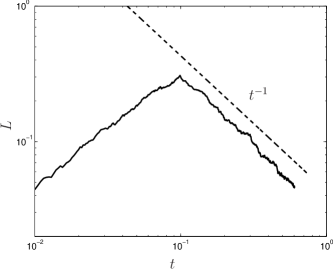
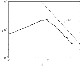
Figure 1: Vortex line density $L$ ($\rm cm^{-2}$) vs time $t$ ($s$) corresponding to small (left) and large (right) times of vortex rings injection. Fitting the decay as $L\sim t^{-\alpha}$, we obtain $\alpha=1.07$ and 1.48, respetively. The dashed lines show the ultraquantum $L\sim t^{-1}$ (left) and quasiclassical $L\sim t^{-3/2}$ (right) behaviours.

observed ultraquantum ($L\sim t^{-1}$) behaviour. During the decay, the kinetic energy (per unit mass), $E$, has the expected $E\sim t^{-1}$ behaviour.

We have repeated the calculation with longer injection time, up to $t=1~{}\rm s$. The peak value of $L$ is thus about 10 times larger than in the ultraquantum case, as in the experiment Walmsley2008 . We have found that, as shown in Fig. 1 (right), after the initial transient the decay assumes the quasiclassical ($L\sim t^{-3/2}$) form observed in the experiments Walmsley2008 ; Bradley2006 . We have also checked that $E\sim t^{-2}$, as expected. The same quasiclassical and ultraquantum decays are obtained with half the numerical resolution along the vortex filaments.

It should be emphasized that left and right of Fig. 1 do not represent different stages of turbulence but reproduce two different experiments Walmsley2008 resulting, respectively, in two different regimes of decay: ultraquantum and quasiclassical. The key parameter, determining which of the two regimes will be realized, is the time of injection of vortex rings.

Assuming the classical expression $dE/dt=-\nu\omega^{2}$, where $\omega$ is the vorticity, and the identification $\omega=\kappa L$, we interpret the results in terms of an effective kinematic viscosity $\nu$, which we call $\nu_{V}$ (“Vinen”) and $\nu_{K}$ (“Kolmogorov”) respectively for the two regimes Walmsley2008 . The values of the effective kinematic viscosities $\nu_{V}$ and $\nu_{K}$ have been obtained as in Ref. Walmsley2008 by fitting respectively $L\approx B/(\nu_{V}t)$, where $B=(1/(4\pi))\ln{(\ell/a_{0})}$ and $a_{0}\approx 10^{-8}~{}\rm cm$ is the vortex core radius, and $L\approx(3C)^{2/3}\nu_{K}^{-1/2}\kappa^{-1}k_{1}^{-1}t^{-3/2}$, where $2\pi/k_{1}$ is the large scale and $C=1.5$ is the Kolmogorov constant. In applying these formulae we have taken into account the fact that for the calculations presented here in the ultraquantum case the computational box is not entirely full, and that in the quasiclassical case the largest length scale is of the order of $0.06~{}\rm cm$, as visible in ${\rm PDF}(C)$. We obtain $\nu_{V}/\kappa\approx 10^{-1}$ and $\nu_{K}/\kappa\approx 10^{-3}$, which compare fairly well with Walmsley & Golov’s $\nu_{V}/\kappa\approx 0.08$ to $0.1$ and $\nu_{K}/\kappa\approx 0.002$ to $0.01$.

To understand the nature of the two regimes we have examined the time behaviour of the probability density function ${\rm PDF}(C)$ (normalized histogram) of the local vortex line curvature, $C=|d^{2}\mathbf{s}/d\xi^{2}|$. In both ultraquantum and quasiclassical case, the initial PDF develops in time to larger and smaller values of $C$. In the quasiclassical case, however, there is a much greater build up at small values of $C$, see Fig. 2; this means that, as the initial vortex rings

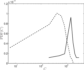
Figure 2: Probability distribution functions of the vortex line curvature, $C$ ($\rm cm^{-1}$). Solid line: ultraquantum decay at $t=0.08~{}\rm s$; dashed line: quasiclassical decay at $t=0.7~{}\rm s$.

entangle, large-scale structures are created consisting of long vortex filaments which can extend across the entire computational domain.

This generation of large length scales is apparent in Fig. 3, where we show the evolution of the kinetic energy

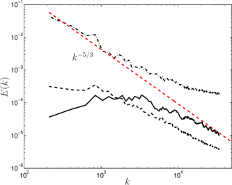
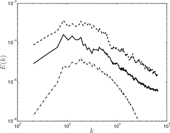
Figure 3: (Color online) Energy spectrum (arbitrary units) vs wavenumber $k$, $\rm cm^{-1}$ corresponding to the quasiclassical decay (left) with the solid line at $t=0.1~{}\rm s$, dot-dashed $t=1.1~{}\rm s$, and dashed $t=3.4~{}\rm s$, and to the ultraquantum decay (right) with the solid line at $t=0.07~{}\rm s$, dashed $t=0.12~{}\rm s$, and dot-dashed $t=0.6~{}\rm s$. In the former, note the formation and decay of the Kolmogorov spectrum (indicated by the straight dashed line).

spectrum $E_{k}$, defined by

$$E=\frac{1}{V}\int_{V}\frac{1}{2}|\mathbf{v}|^{2}\,dV=\int_{0}^{\infty}E_{k}\,dk$$ (2)

(where $V$ is volume and $k$ the magnitude of the three-dimensional wavevector $\bf k$). In both ultraquantum and quasiclassical cases the energy is initially concentrated at intermediate wavenumbers. It is apparent (see Fig. 3 right) that in the ultraquantum case the value of $k=k_{*}$, where $E_{k}$ has the maximum does not change, and the ratio of energy transferred to large scales, $\int_{0}^{k_{*}}E_{k}\,dk$, to that transferred to small scales, $\int_{k_{*}}^{\infty}E_{k}\,dk$, remains small ($<0.13$) at all times. In the quasiclassical case, however, a significant amount of energy is transferred to small wavenumbers, leading to the formation of the Kolmogorov $k^{-5/3}$ spectrum, see Fig. 3. The spectrum maintains the Kolmogorov scaling during the decay stage, consistently with the observation that $L\sim t^{-3/2}$, even for relatively small values of $L$ which would otherwise decay as $t^{-1}$ if $L$ were small initially.

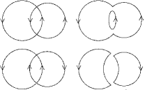
Figure 4: Head-on reconnection of two vortex rings of similar size tends to produce two vortex loops of similar size (bottom), whereas the reconnection of two rings traveling in the same direction produces one vortex loop which is much smaller and one which is much bigger (top).

To interpret these results we remark that in both experiments Walmsley2008 ; Bradley2006 the initial vortex rings do not move isotropically, but essentially travel in the same direction as a beam. This anisotropy is important in creating large length scales, provided that the initial density of the rings is large enough. The argument is the following. Energy and speed of a vortex ring of radius $R$ are respectively proportional and inversely proportional to $R$. Consider the collision of two vortex rings of approximately the same size. If the collision is head-on, the outcome of the reconnection will be two vortex loops of approximately the same size, as shown schematically in Fig. 4 (bottom). If the two rings travel approximately in the same direction, the reconnection will create two vortex loops, one small and one big, see Fig. 4 (top). To test the idea that an anisotropic beam facilitates the creation of length scales, we have performed numerical calculations in which the initial distribution of vortex rings differs only by the orientation of the rings: in one case the rings pointed isotropically in all directions, and in another case they pointed in the same direction.

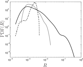
Figure 5: Probability distribution functions, PDF($R$) of loop sizes $R$, ($\rm cm$). Dashed line: initial PDF. Grey line: resulting PDF for isotropic initial condition: no large loops are created by the vortex reconnections. Black line: resulting PDF for anisotropic initial condition: note the generation of large loops.

Figure 5 confirms that the anisotropic initial condition generates smaller values of curvature (that is, larger length scales) as well as bigger ones. To highlight the geometrical role of vortex reconnections, the calculation was performed by replacing Eq. (1) with the local induction approximation Saffman1992 $d{\bf s}/dt=\beta{\bf s}^{\prime}\times{\bf s}^{\prime\prime}$ (where the prime denotes derivative with respect to arclength and $\beta$ is constant); in this way the rings interacted only when they collided. The result was similar to that obtained using the full Biot-Savart calculation.

In conclusion, our model reproduces both the ultraquantum ($L\sim t^{-1}$) and the quasiclassical ($L\sim t^{-3/2}$) turbulent decay regimes which have been observed in the experiments Walmsley2008 ; Bradley2006 and explains their hydrodynamical natures. By examining the curvature PDF and the energy spectrum, we have found that in the quasiclassical regime the initial energy distribution is shifted to large scales, and a Kolmogorov spectrum is formed. In the ultraquantum case, the spectrum decays without this energy transfer. In the case where turbulence is generated by forcing in the vicinity of some (intermediate) lengthscale, as in the experiments Walmsley2008 ; Bradley2006 , we found that the ultraquantum regime is induced only if the total energy input is relatively low, while the higher energy input (by e.g. the prolonged injection of the vortex rings in experiments Walmsley2008 ; Bradley2006 ) generates the large scale motion and hence the quasiclassical, Kolmogorov regime of turbulence. We have also found that the anisotropy of the beam of vortex rings is important, as reconnections of vortex loops traveling in the same direction are very effective in creating larger length scales.

- (1) W. F. Vinen and J. J. Niemela, J. Low Temp. Phys. 128, 167 (2002).
- (2) P. M. Walmsley and A. I. Golov, Phys. Rev. Lett. 100, 245301 (2008).
- (3) D. I. Bradley et al. , Phys. Rev. Lett. 96, 035301 (2006).
- (4) D. I. Bradley et al. , Nature Physics 7, 437 (2011).
- (5) L. Ts. Adzhemyan, M. Hnatich, D. Horváth, and M. Stehlich, Phys. Rev. E 58, 4511 (1998).
- (6) C. Nore, M. Abid, and M. E. Brachet, Phys. Rev. Lett. 78, 3896 (1997).
- (7) J. Maurer and P. Tabeling, Europhys. Lett. 43, 29 (1998).
- (8) M. Kobayashi and M. Tsubota, Phys. Rev. Lett. 94, 065302 (2005).
- (9) V. S. L’vov, S. V. Nazarenko, and L. Skrbek, Low Temp. Phys. 145, 125 (2006).
- (10) J. Salort et al. , Phys. Fluids 22, 125102 (2010).
- (11) N. B. Kopnin, G. E. Volovik, and U. Parts, Europhys. Lett. 32, 651 (1995).
- (12) G. E. Volovik, JETP Lett. 78, 553 (2003).
- (13) L. Skrbek, JETP Lett. 80, 474 (2006).
- (14) T. Winiecki and C. S. Adams, Europhys. Lett. 52, 257 (2000).
- (15) P. M. Walmsley, A. I. Golov, H. E. Hall, A. A. Levchenko, and W. F. Vinen, Phys. Rev. Lett. 99, 265302 (2007).
- (16) S. R. Stalp, L. Skrbek, and R. J. Donnelly, Phys. Rev. Lett. 82, 4831 (1999).
- (17) S. Fujiyama et al. , Phys. Rev. B 81, 180512(R) (2010).
- (18) K. W. Schwarz, Phys. Rev. B 38, 2398 (1988).
- (19) P. G. Saffman, Vortex Dynamics (Cambridge Univ. Press, Cambridge, 1992).
- (20) D. I. Bradley et al. , Phys. Rev. Lett. 95, 035302 (2005).
- (21) A. W. Baggaley and C. F. Barenghi, Phys. Rev. B 83, 134509 (2011).
- (22) A. W. Baggaley and C. F. Barenghi, Phys. Rev. B 84, 020504 (2011).
- (23) A. W. Baggaley and C. F. Barenghi, J. Low Temp. Physics 166 3–20 (2012).
- (24) M. Leadbeater, T. Winiecki, D. C. Samuels, C. F. Barenghi, and C. S. Adams, Phys. Rev. Lett. 86 1410–1413 (2001).